Recent ozone trends in the Chinese free troposphere: role of the local emission reductions and meteorology

Free tropospheric ozone (O₃) trends in the Central East China (CEC) and export regions are investigated for 2008–2017 using the IASI (Infrared Atmospheric Sounding Interferometer) O₃ observations and the LMDZ-OR-INCA model simulations, including the most recent Chinese emission inventory. The observed and modelled trends in the CEC region are −0.07 ± 0.02 and −0.08 ± 0.02 DU yr⁻¹, respectively, for the lower free troposphere (3–6 km column) and −0.05 ± 0.02 and −0.06 ± 0.02 DU yr⁻¹, respectively, for the upper free troposphere (6–9 km column). The statistical p value is smaller to 0.01 for all the derived trends. A good agreement between the observations and the model is also observed in the region, including the Korean Peninsula and Japan and corresponding to the region of pollution export from China. Based on sensitivity studies conducted with the model, we evaluate, at 60 % and 52 %, the contribution of the Chinese anthropogenic emissions to the trend in the lower and upper free troposphere, respectively. The second main contribution to the trend is the meteorological variability (34 % and 50 %, respectively). These results suggest that the reduction in NO_x anthropogenic emissions that has occurred since 2013 in China led to a decrease in ozone in the Chinese free troposphere, contrary to the increase in ozone at the surface. We designed some tests to compare the trends derived by the IASI observations and the model to independent measurements, such as the In-service Aircraft for a Global Observing System (IAGOS) or other satellite measurements (Ozone Monitoring Instrument (OMI)/Microwave Limb Sounder (MLS)). These comparisons do not confirm the O₃ decrease and stress the difficulty in analysing short-term trends using multiple data sets with various sampling and the risk of overinterpreting the results.

1 Introduction

Tropospheric ozone is a harmful pollutant close to the surface impacting human health and ecosystems (Lelieveld et al., 2015; Monks et al., 2015). Tropospheric ozone is also a short-lived climate forcer with an impact on surface temperature that is greatest in the upper troposphere lower stratosphere (UTLS) and then contributes to climate change (Riese et al., 2012). The recent Tropospheric Ozone Assessment Report (TOAR) has stated that free tropospheric O₃ increased during industrial times and the last few decades (Gaudel et al., 2018; Tarasick et al., 2019). At the surface, the trends depend on the following considered regions: a decrease is observed during summertime in North America and in Europe and an increase is observed in Asia (e.g. Gaudel et al., 2018, 2020). However, conclusions are more difficult to draw for the recent trends of tropospheric ozone. In addition to the statistical robustness of these trends, Gaudel et al. (2018) point out inconsistencies between satellite trends derived from ultraviolet (UV) sounders, which show mainly positive trends (e.g. Cooper et al., 2014; Ziemke et al., 2019) and infrared (IR) sounders, which show mainly negative trends (Wespes et al., 2017).

In China and Central East China (CEC), one of the most polluted regions worldwide (e.g. Wang et al., 2017; Fan et al., 2020), stringent pollutant emission controls for NO_x, SO₂, and primary PM (particulate matter) emissions have been enacted during the last decade (Zhang et al., 2019; Zheng et al., 2018). The main objective of these restrictions was to decrease primary and secondary PM concentrations (e.g. Zhai et al., 2019; Zhang et al., 2019). However, these reductions have led to a worsening of urban ozone pollution (e.g. Li et al., 2020; Liu and Wang, 2020a, b; Lu et al., 2018; Ma et al., 2021; Chen et al., 2021), attributed to O₃ precursors reductions in the large urban volatile organic carbon (VOC)-limited regions and indirectly to the aerosol reductions, which slow down the aerosol sink of hydroperoxy radicals (RO₂) and then increase the ozone production (Li et al., 2019; Ma et al., 2021). Most of the studies are based on surface observations and model simulations.

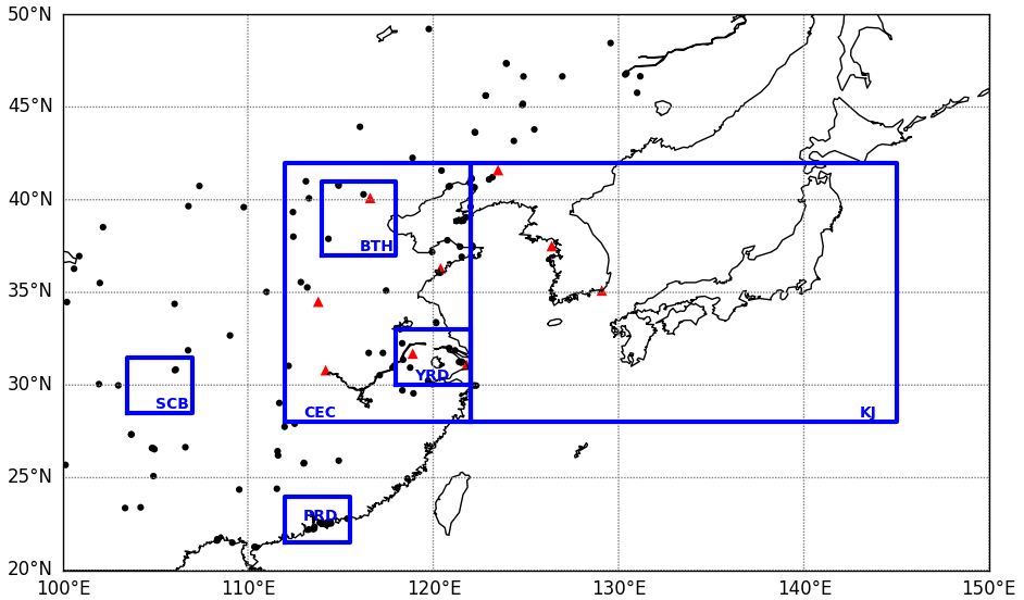
Figure 1 The northeastern Asian domain of the study. The following six subregions of interest are considered: Central East China (CEC; 28–42^∘ N, 112–122^∘ E), the Beijing–Tianjin–Hebei region (BTH; 37–41^∘ N, 114–118^∘ E), the Yangtze River Delta (YRD; 30–33^∘ N, 118–122^∘ E), the Pearl River Delta (PRD; 21.5–24^∘ N, 112–115.5^∘ E), the Sichuan Basin (SCB; 28.5–31.5^∘ N, 103.5–107^∘ E), and the Korean Peninsula–Japan region (KJ; 28–42^∘ N, 122–145^∘ E). Black circles show the rural-type surface stations and the red triangles the IAGOS airports used in this study.

Satellite observations are more difficult to use to derive information on surface ozone due to their lack of sensitivity to surface concentration. Shen et al. (2019) show a relatively good correlation between Ozone Monitoring Instruments (OMIs) and surface measurements, especially in southern China, and state a possibility to infer trends for the subtropical latitudes. This was already partly reported by Hayashida et al. (2015). For individual events, IASI (Infrared Atmospheric Sounding Interferometer; Dufour et al., 2015) and IASI + GOME2 (Cuesta et al., 2018) products show the ability to inform on pollution events in the North China Plain (NCP). The IASI + GOME2 O₃ product shows a better ability to reproduce ozone surface concentrations, with good comparisons with surface measurements in Japan (Cuesta et al., 2018). Despite this encouraging partial sensitivity to the surface or boundary layer ozone, satellite observations such as IASI are mostly suited to probe free tropospheric ozone. IASI is, however, able to separate, at least partly, the information from the lower and the upper troposphere with a maximum of sensitivity between 3 and 6 km (Dufour et al., 2010, 2012, 2015). Based on the IASI observations, Dufour et al. (2018) discuss lower tropospheric O₃ trends (surf–6 km) over the NCP for the 2008–2016 period and associate driving factors using a multivariate regression model. They show that the O₃ trend derived from IASI is negative (−0.24 DU yr⁻¹ or −1.2 % yr⁻¹) and explained by large-scale dynamical processes, such as El Niño and changes in precursors emissions, that have occurred since 2013. The hypothesis to explain the negative impact of precursors reduction compared to the positive one at the surface is related to the chemical regime turning from VOC limited at the surface to NO_x limited in altitude. In this study, we examine the ability of IASI to derive free tropospheric ozone trends in China by comparison with the state-of-the-art global chemistry climate model LMDZ-OR-INCA for the 2008–2017 period. Satellite observations and the model are evaluated using independent observations (surface measurements, In-service Aircraft for a Global Observing System (IAGOS) aircraft measurements, and ozonesondes). We use the model to quantify, independently from IASI, the contributions of local anthropogenic emissions and other possible driving factors (meteorology, global anthropogenic emissions, biomass burning, and methane). Results are also contrasted with the Gaudel et al. (2018) TOAR outcomes. The domain and regions of interest of our study are shown in Fig. 1. Section 2 provides a description of the different satellite and in situ data and the chemical climate model. The IASI ozone product and the model simulations are evaluated against independent in situ measurements and compared in Sect. 3. Section 4 presents the observed and simulated O₃ trends in the troposphere. The results are discussed in Sect. 5.

2 Data and model description

2.1 IASI satellite data and ozone retrieval

The IASI (Infrared Atmospheric Sounding Interferometer) instruments are nadir-viewing Fourier transform spectrometers. They are flying on board the EUMETSAT (European Organisation for the Exploitation of Meteorological Satellites) Metop satellites (Clerbaux et al., 2009). In total, three versions of the instrument are currently operational on the same orbit: one has been aboard the Metop-A platform since October 2006, one has been aboard the Metop-B platform since September 2012, and one has been aboard the Metop-C platform since November 2018. The IASI instruments operate in the thermal infrared between 645 and 2760 cm⁻¹, with an apodised resolution of 0.5 cm⁻¹. The field of view of the instrument is composed of a 2 × 2 matrix of pixels with a diameter at nadir of 12 km each. IASI scans the atmosphere with a swath width of 2200 km and crosses the Equator at two fixed local solar times 09:30 LT (descending mode) and 21:30 LT (ascending mode), allowing the monitoring of atmospheric composition twice a day at any location.

Ozone profiles are retrieved from the IASI radiances using the Karlsruhe Optimized and Precise Radiative transfer Algorithm (KOPRA) radiative transfer model, its inversion tool (KOPRAFIT), and an analytical altitude-dependent regularisation method, as described in Eremenko et al. (2008) and Dufour et al. (2012, 2015). In order to avoid the potential impact of versioning of the auxiliary parameters (such as temperature profile, clouds screening, etc.) on the ozone retrieval (Van Damme et al., 2017), surface temperature and temperature profiles are retrieved before the ozone retrieval. A data screening procedure is applied to filter cloudy scenes and to ensure the data quality (Eremenko et al., 2008; Dufour et al., 2010, 2012). The a priori and the constraints are different, depending on the tropopause height, which is based on the 2 PV geopotential height product from the ECMWF (European Centre for Medium-Range Weather Forecasts). There is one a priori and one constraint used for polar situations (i.e. tropopause < 10 km), one for midlatitude situations (i.e. tropopause within 10–14 km), and one for tropical situations (i.e. tropopause > 14 km). The a priori profiles are compiled from the ozonesonde climatology of McPeters et al. (2007). Compared to the previous version of the ozone product (Dufour et al., 2018), water vapour is fitted simultaneously with ozone to account for remaining interferences in the spectral windows used for the retrieval and to improve the retrieval in the current version (3.0) of the product. From the retrieved profiles, different ozone partial columns can be calculated. In this study, we consider the following four partial columns: the lowermost tropospheric (LMT) column from the surface to 3 km (named 0–3 km), the lower free tropospheric (LFT) column from 3 to 6 km (named 3–6 km), the upper free tropospheric (UFT) column from 6 to 9 km (named 6–9 km), and the upper tropospheric–lowermost stratospheric (UT-LMS) column from 9 to 12 km (named 9–12 km). Note that only the morning overpasses of IASI are considered for this study in order to remain in thermal conditions with a better sensitivity to the lower troposphere. To cover a larger period, we also consider only IASI on Metop-A. Initial validation of the KOPRAFIT IASI ozone retrievals with ozonesondes and IAGOS data is presented in Sect. 3.

2.2 Ozonesondes

Ozonesondes measure in situ vertical profiles of temperature, pressure, humidity, and ozone up to 30–35 km, with a vertical resolution of ∼ 150 m for ozone. The ozonesondes data come mainly from the World Ozone and Ultraviolet Radiation Data Centre (WOUDC) database (http://www.woudc.org/, last access: 19 October 2021), and the Southern Hemisphere Additional Ozonesondes (SHADOZ) database (http://croc.gsfc.nasa.gov/shadoz/, last access: 19 October 2021). The sonde measurements use electrochemical concentration cell (ECC) technique, relying on the oxidation of ozone with a potassium iodine (KI) solution (Komhyr et al., 1995), except the Hohenpeißenberg sondes, which use Brewer–Mast-type sondes. Their accuracy for the ozone concentration measurement is about ± 5 % (Deshler et al., 2008; Smit et al., 2007; Thompson et al., 2003). We use a database of ozonesonde measurements from 2007 to 2012, including 24 stations in the midlatitudinal bands (30–60^∘; both hemispheres), 13 stations in the tropical band (30^∘ S–30^∘ N) and 16 stations in the polar bands (60–90^∘; both hemispheres). A list of stations and related information is provided in Table A1 (Appendix A).

2.3 Surface measurements

Observational data are issued from the China National Environmental Monitoring Centre (CNEMC) and archived at https://quotsoft.net/air/ (last access: 3 May 2021). The data set provides hourly data of criteria pollutants SO₂, O₃, NO₂, CO, PM_2.5, and PM₁₀ consolidated every day in near-real time from May 2014. It has been used in several other studies (e.g. Li et al., 2020; Yin et al., 2021). Only national-level data are available in this data set for about 1300 stations throughout mainland China. In this study, we consider only the stations with more than 50 % of measurements available to ensure a good temporal coverage for the entire period (2014–2017). In the domain shown in Fig. 1, this corresponds to 685 stations. We classified the stations in the following different types of environment: mountain, rural, suburban, urban, and traffic, based on the approach developed by Flemming et al. (2005) for Europe. This method has the advantage of not requiring any additional information other than the pollutant concentration. The relative amplitude of the diurnal cycle of O₃ observations is used to evaluate the representative environment of the station, with the assumption that the larger the amplitude of the diurnal ozone cycle is, the more the station is in an urban environment. In our case, each station has been evaluated during the studied period (i.e. 2014–2017).

2.4 IAGOS data

IAGOS (In-Service Aircraft for Global Observing System; http://www.iagos.org, last access: 19 October 2021) is a European research infrastructure dedicated to measuring air composition (Petzold et al., 2016). The programme counts more than 62 000 flights between 1994 and 2021 with ozone measurements. For the purpose of this study, we used all profiles of ozone at any time of day available above northeastern China/Korean Peninsula between 2011 and 2017. On board the IAGOS commercial aircraft, ozone is measured using dual-beam ultraviolet absorption monitor (time resolution of 4 s), with an accuracy and a precision estimated at about 2 nmol mol⁻¹ and 2 %, respectively. Further information on the instrument is available in other articles (see Thouret et al., 1998; Nédélec et al., 2015). Long-term quality and consistency have been assessed by Blot et al. (2021).

2.5 OMI/MLS

Ozone Monitoring Instrument (OMI)/Microwave Limb Sounder (MLS) tropospheric column ozone is described by Ziemke et al. (2019). The OMI/MLS ozone product represents monthly means for October 2004 to the present at 1^∘ × 1.25^∘ resolution and a latitude range of 60^∘ S–60^∘ N. Tropospheric column ozone is determined by subtracting co-located Microwave Limb Sounder (MLS) stratospheric column ozone from OMI total column ozone each day at each grid point. Tropopause pressure used to determine MLS stratospheric column ozone invoked the WMO (World Meteorological Organization) 2 K km⁻¹ lapse rate definition from National Centers for Environmental Prediction (NCEP) re-analyses. OMI total ozone data are available from https://ozonewatch.gsfc.nasa.gov/data/omi/ (last access: 22 April 2021). MLS ozone data can be obtained from https://mls.jpl.nasa.gov (last access: 19 October 2021). Estimated 1σ precision for the OMI/MLS monthly mean gridded tropospheric columns of ozone (TCO) product is 1.3 DU.

2.6 LMDZ-OR-INCA model

The LMDZ-OR-INCA global chemistry–aerosol–climate model (hereafter referred to as INCA – INteraction with Chemistry and Aerosols) couples the LMDZ (Laboratoire de Météorologie Dynamique; version 6) general circulation model (GCM; Hourdin et al., 2006), and the INCA (version 5) model online (Hauglustaine et al., 2004). The interaction between the atmosphere and the land surface is ensured through the coupling of LMDZ with the ORCHIDEE (ORganizing Carbon and Hydrology In Dynamic Ecosystems; version 9) dynamical vegetation model (Krinner et al., 2005). In the present configuration, the model includes 39 hybrid vertical levels extending up to 70 km. The horizontal resolution is 1.25^∘ in latitude and 2.5^∘ in longitude. The primitive equations in the GCM are solved with a 3 min time step, large-scale transport of tracers is carried out every 15 min, and physical and chemical processes are calculated at a 30 min time interval. For a more detailed description and an extended evaluation of the GCM, we refer to Hourdin et al. (2006). INCA initially included a state-of-the-art CH₄-NO_x-CO-NMHC-O₃ tropospheric photochemistry (Hauglustaine et al., 2004; Folberth et al., 2006). The tropospheric photochemistry and aerosols scheme used in this model version is described through a total of 123 tracers, including 22 tracers to represent aerosols. The model includes 234 homogeneous chemical reactions, 43 photolytic reactions, and 30 heterogeneous reactions. Please refer to Hauglustaine et al. (2004) and Folberth et al. (2006) for the list of reactions included in the tropospheric chemistry scheme. The gas-phase version of the model has been extensively compared to observations in the lower troposphere and in the upper troposphere. For aerosols, the INCA model simulates the distribution of aerosols with anthropogenic sources such as sulfates, nitrates, black carbon, and particulate organic matter, as well as natural aerosols such as sea salt and dust. Ammonia and nitrates aerosols are considered as described by Hauglustaine et al. (2014). The model has been extended to include an interactive chemistry in the stratosphere and mesosphere (Terrenoire et al., 2021). Chemical species and reactions specific to the middle atmosphere were added to the model. A total of 31 species were added to the standard chemical scheme, mostly belonging to the chlorine and bromine chemistry, and 66 gas-phase reactions and 26 photolytic reactions.

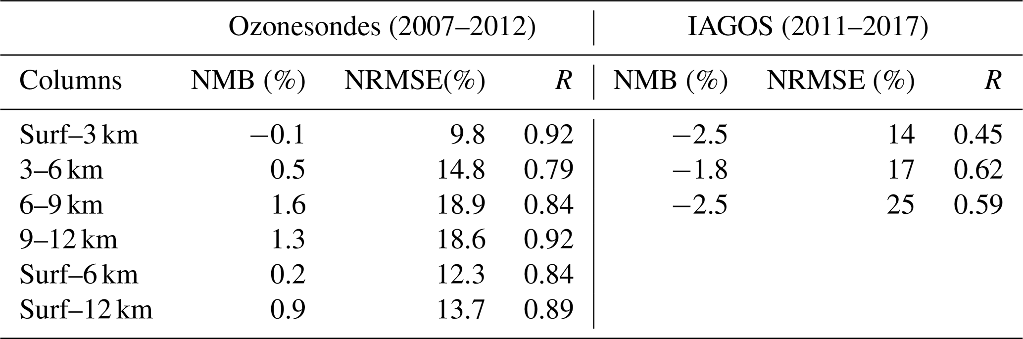
Table 1 Statistics of the comparison of different O₃ partial columns derived from IASI with O₃ partial columns measured with ozonesondes for 2007–2012 all the globe and with IAGOS for 2011–2017 for North China–Korean Peninsula. The normalised mean bias (NMB), the normalised root mean square error (NRMSE), and the Pearson correlation coefficient (R) are provided.

In this study, meteorological data from the European Centre for Medium-Range Weather Forecasts (ECMWF) ERA-Interim reanalysis have been used to constrain the GCM meteorology and allow a comparison with measurements. The relaxation of the GCM winds towards ECMWF meteorology is performed by applying, at each time step, a correction term to the GCM u and v wind components, with a relaxation time of 2.5 h (Hauglustaine et al., 2004). The ECMWF fields are provided every 6 h and interpolated onto the LMDZ grid.

The historical global anthropogenic emissions are taken from the Community Emissions Data System (CEDS) inventories (Hoesly et al., 2018) up to 2014. After 2014, the global anthropogenic emissions are based on Gidden et al. (2019). For China, the anthropogenic emission inventories are replaced the MEIC (Multi-resolution Emission Inventory for China) inventory (Zheng et al., 2018) available for the period 2010–2017. The global biomass burning emissions are taken from van Marle et al. (2017) up to 2015 and from Gidden et al. (2019) after 2015. The ORCHIDEE vegetation model has been used to calculate the biogenic surface fluxes of isoprene, terpenes, acetone, and methanol, as well as NO soil emissions as described by Messina et al. (2016), offline.

3 Evaluation of the IASI O₃ satellite product and model simulations

3.1 Validation of the IASI O₃ product with ozonesondes and IAGOS

We present here a short validation of the version 3.0 of the IASI O₃ product developed at Laboratoire Interuniversitaire des Systèmes Atmosphériques (LISA). A detailed validation will be provided in a dedicated paper. The coincidence criteria used for the validation are 1^∘ around the station, a time difference shorter than ± 6 h, and a minimum of 10 clear-sky pixels matching these criteria. No correction factor has been applied on ozonesonde measurements as our main concern is the (lower) troposphere. The results of the comparison between IASI ozone retrievals and ozonesonde measurements are summarised in Table 1 for different partial columns in the troposphere. Normalised mean biases (NMB) for the different partial columns remain very small (< 2 %). The estimated errors given by the normalised root mean square error (NRMSE) range between 10 % and 20 %, depending on the partial columns, and the Pearson correlation coefficient (R) is larger than or equal to 0.79. Note that these results are based on the comparison with ozonesonde profiles smoothed by the averaging kernels of the IASI retrieval. If we compare with the raw sonde profiles without any smoothing, the results are slightly degraded but remain good, with the normalised biases within ± 5 %, the errors smaller than 30 %, and the correlations larger than 0.6. Version 3.0 of the O₃ IASI product reduces biases and increases the correlation with the ozonesondes measurements. The bias reduction is the most effective in the upper troposphere.

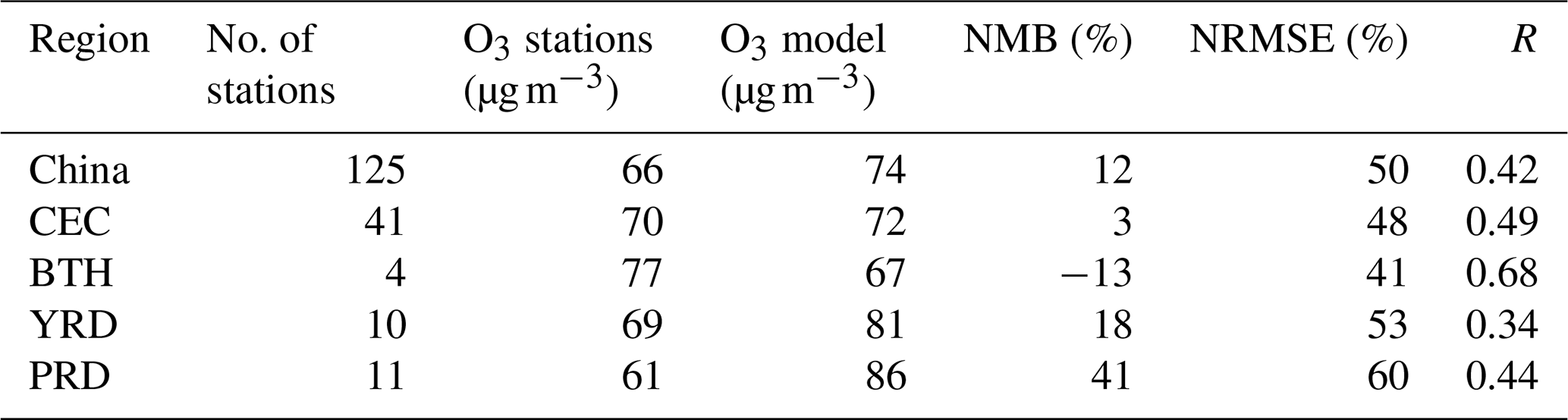
Table 2 Comparison between the daily O₃ concentrations simulated by the INCA model and the daily mean O₃ concentrations measured at the Chinese surface stations for 2014–2017. Due to the model resolution, only the stations classified as rural are used for the comparison. For each region, the number of stations and the mean observed and simulated O₃ concentrations are provided. The normalised mean bias (NMB in percent) is calculated as the difference between the model concentration and the observed one, with the latter used as the reference. The normalised root mean square error (NRMSE in percent) is calculated based on the daily averages, and the correlation coefficient (R) corresponds to the temporal and the spatial correlation (the daily time series of each station are considered in its calculation without any regional averaging).

In addition, we compared IASI ozone partial columns with IAGOS ozone partial columns calculated from profiles measured above Chinese and Korean Peninsula airports for the period 2011–2017. In this region, the IAGOS coverage was too sparse before this period. IAGOS profiles are filtered to coincidence in space and time, with IASI pixels using the same criteria as for the ozonesondes (1^∘ around the station; ± 6 h). The reference point for IAGOS to apply the coincidence criteria is the middle of the profile. IAGOS profiles with data missing above 500 hPa do not extend enough in altitude to be correctly compared to IASI observations, and then they are not analysed. After these two filters, we count 213 IAGOS profiles for the time period 2011–2017. These selected profiles are extended vertically between the top (usually the cruise altitude of the aircraft) and 60 km, with the a priori profiles used in the IASI retrieval. We apply the IASI averaging kernels to these extended IAGOS profiles. The 500 hPa criterion to filter the IAGOS profiles is a compromise to have a reasonable number of profiles to compare with and to limit the contribution of a priori in the lower tropospheric part of the smoothed profiles. Despite this, the resulting smoothed IAGOS profile may still be significantly affected by the a priori profile used to extend the raw IAGOS profile, especially when the cruise altitude of the profile is low. Then, the comparison between IASI and IAGOS is the most meaningful below 500 hPa and for the partial columns representative of the lower free troposphere. We focus more on the lower free tropospheric column (3–6 km) where the IASI retrievals are the most sensitive to ozone (Dufour et al., 2012). Results are summarised in Table 1. The normalised mean bias and the normalised root mean square error estimate between IASI and IAGOS are −1.8 % and 17 %, respectively when averaging kernels (AKs) are applied to IAGOS profiles (−5.6 % and 18 % without AKs applied) for this column, which is in agreement with global ozonesonde validation. The correlation is smaller (0.62) than the one with the sondes (0.79). Statistics for the other columns are also reported in Table 1. The agreement is still good in terms of bias in the LMT (0–3 km) column but degrades in terms of correlation. The temporal coincident criterion (± 6 h) combined with a non-negligible influence of the ozone diurnal cycle (Petetin et al., 2016) on the LMT (0–3 km) column might explain the lower correlation for this column (0.45). In addition, the comparison made assuming a vertical profile at the latitude and longitude of the midpoint of a slant profile recorded during take-off and landing phases. The lowest part of the profile may be more influenced by urban areas near the airport and then be less reproduced by IASI due to its limited sensitivity close to the surface. For the 6–9 km column, only 50 profiles over 213 reach 300 hPa, and then the IAGOS profiles are largely mixed with the a priori profile used in the IASI retrieval. The evaluation of IASI using IAGOS is then difficult for the 6–9 km column with so few coincident observations.

3.2 Evaluation of the INCA simulations

The model is evaluated using the Chinese surface network described in Sect. 2.3. As the model resolution is coarse and not representative of urban situations, we compare the model only with the rural-type stations. The daily O₃ concentrations simulated by the model are compared to the daily averages calculated from the hourly surface measurements provided by the Chinese surface network. The normalised mean bias between INCA and the surface stations is 12 % over the Chinese domain considered, with INCA being larger. The correlation and the normalised root mean square error (NRMSE) are 0.42 % and 50 %, respectively. On average, the model shows relatively good performances, especially in terms of bias. However, the performances of the model in reproducing the ozone concentration depend on the region. A good agreement is observed in the CEC region, with a bias of 3 %, correlation of 0.49, and NRMSE of 48 %, respectively (Table 2). In the BTH region, north of the CEC, the modelled O₃ concentrations are smaller than the observed ones (−13 %), but the correlation is higher (0.68). In the south of the CEC, the comparison in the YRD region remains satisfying in terms of bias (18 %) but is degraded for the correlation (0.34) and the NRMSE (53 %). In the coastal region of PRD, the available stations are within one model grid cell, including land and sea. The coarse resolution of the model likely limits its capability to reproduce correctly the O₃ concentrations of the coastal stations: the model overestimates the surface measurements (41 %) with large NRMSE (60 %) and poor correlation (0.44). In the SCB, too few stations are available to provide statistics for the comparison. Figure A1 (Appendix A) shows the comparison station by station. Similar results are shown with a very good agreement in the northern part of the domain; biases are within 10 %, correlation is larger than 0.6, and NRMSE is smaller than 40 %. In the southern part of the domain, the model has some difficulties in reproducing the observations, with biases ranging from 30 % to 60 % for most of the stations and being larger for some stations. The correlation is limited, and the NRMSE is larger than 50 %. In terms of trends, the 2014–2017 time period is short to derive robust trends. When considering observed and simulated trends at the surface with p values smaller than 0.05, model and observations are rather consistent, especially in regions where the model simulates the O₃ concentrations correctly (Fig. A2). The model tends to underestimate the positive trends compared to the observations.

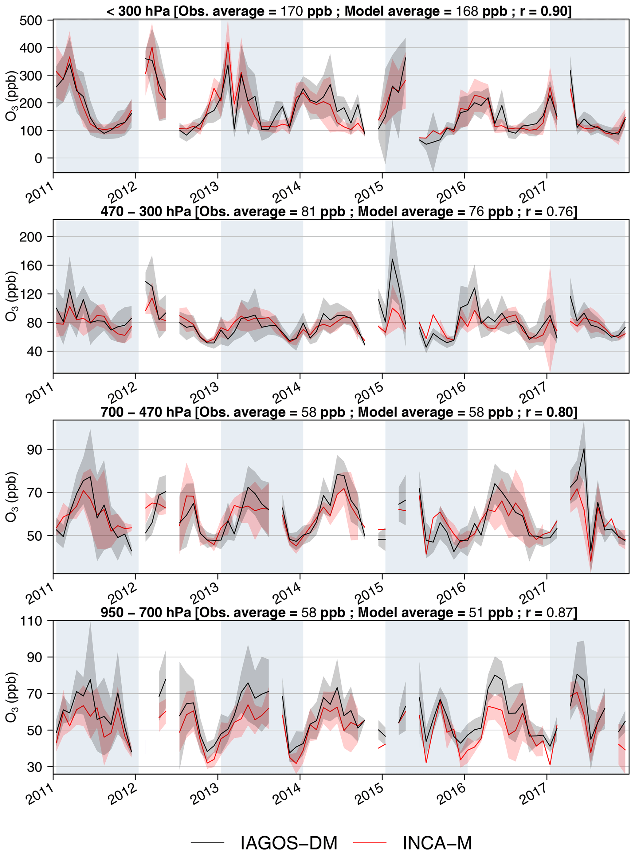
Figure 2 Ozone monthly mean values derived in four altitude domains representing the LMT, LFT, UFT, and UT-LMS (from bottom to top) from the gridded IAGOS data set (solid black line) and the simulation output (solid red line) over northeastern Asia, with respect to the IAGOS mask. The uncertainties are defined by the regional average of the standard deviations calculated for each grid cell. For each altitude domain, the yearly O₃ concentration derived from the mean seasonal cycle is indicated above the corresponding graphic for both data sets, with the Pearson correlation coefficient comparing the two monthly time series.

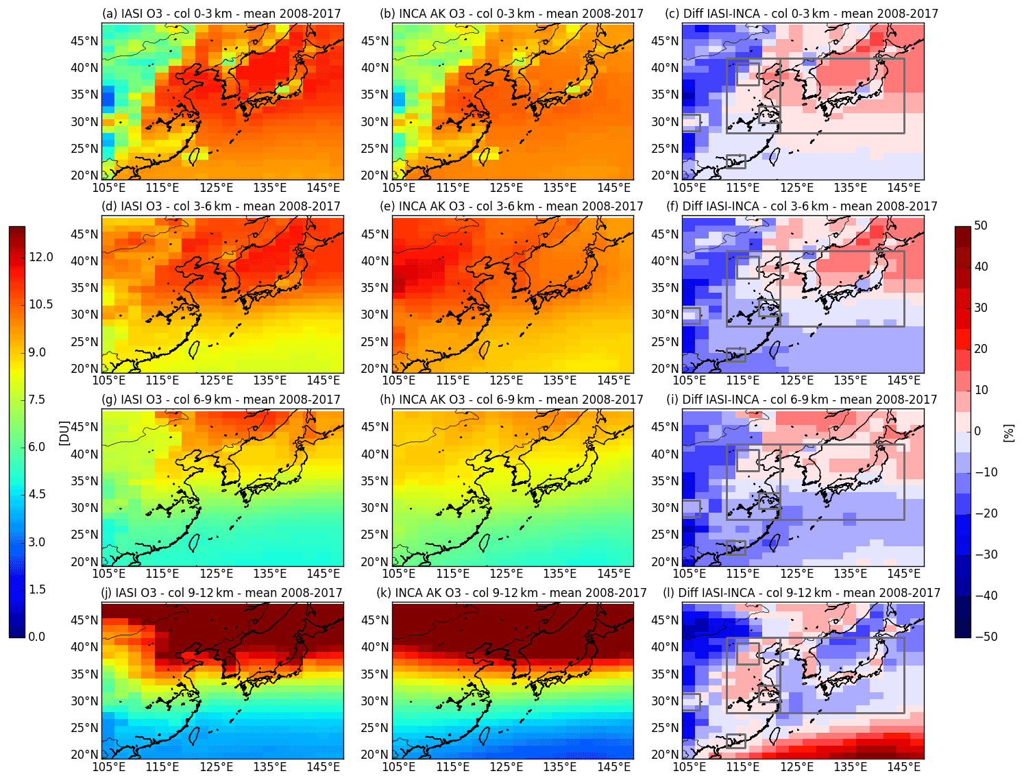
Figure 3 Mean O₃ partial columns for 2008–2017 observed with IASI (a, d, g, and j), simulated by INCA (b, e, h, and k), and their differences (c, f, i, and l). The INCA ozone profiles are smoothed by each individual IASI AKs. The following different partial columns are considered: the lowermost tropospheric columns from the surface to 3 km altitude (named 0–3 km), the lower free tropospheric columns from 3 to 6 km altitude (named 3–6 km), the upper free tropospheric column from 6 to 9 km (named 6–9 km), and the upper tropospheric column from 9 to 12 km (named 9–12 km).

We use also IAGOS ozone profiles above Chinese and Korean Peninsula airports for the period 2011–2017 to evaluate the model above 950 hPa (Fig. 2). The selected IAGOS data correspond to the lowermost troposphere (950–700 hPa), the lower (700–470 hPa) and upper (470–300 hPa) free troposphere, and the UT-LMS (< 300 hPa) above the Chinese coast (east of 110^∘ E and between 30 and 50^∘ N) and South Korea. In order to assess more precisely the model's ability to reproduce the observed ozone behaviour, the IAGOS data are projected onto the model daily grid using the Interpol-IAGOS software (Cohen et al., 2021a) and averaged every month. The subsequent product is hereafter called IAGOS-DM (Distributed onto the Model grid). We derive monthly means from the INCA daily output by selecting the sampled grid cells. These monthly fields are called INCA-M (with M referring to the IAGOS mask). The two products IAGOS-DM and INCA-M are, thus, consistent in space and time and can be compared together. It is important to note that the regional averages calculated here do not account for the tropopause altitude, in contrast to Cohen et al. (2021a). Last, as in Cohen et al. (2018), the statistical representativeness of the observations is enhanced by filtering out the regional monthly means either with fewer than 300 measurement points or fewer than 7 d separating the first and the last measurements. A very good agreement is observed between the INCA model and the IAGOS observations, with small biases ranging from 1.6 % in the lower free troposphere to 12 % in the lowermost troposphere. The INCA and IAGOS time series are well correlated with correlation coefficients equal to or larger than 0.76. Looking in detail, the time series shows that the model tends to underestimate O₃ in the lowermost troposphere and to underestimate the largest O₃values in the lower and the upper free troposphere.

Figure 4 IASI and INCA monthly time series (a, c, e, and g) and anomalies (b, d, f, and h) for the 0–3, 3–6, 6–9, and 9–12 km O₃ partial columns over the CEC region for 2008–2017. Biases, RMSE, and Pearson correlation coefficient between the IASI and INCA monthly time series are provided, as well as the trends, uncertainties, and associated p values calculated from the anomalies time series.

Figure 5 Trends calculated in percent per year at the 2.5^∘ × 1.25^∘ resolution for the 0–3, 3–6, 6–9, and 9–12 km O₃ partial columns. Panels (a, e, i, and m) show the trends derived from IASI, panels (b, f, j, and n) show the trends derived from INCA sampled over the IASI pixels, panels (c, g, k, and o) show the trends derived from INCA with its native daily resolution, and panels (d, h, l, and p) show the trends derived from the INCA reference simulation minus the MET simulation (see the text and Table 4 for details). White crosses are displayed when p values are smaller than 0.05.

3.3 Comparison between IASI O₃ product and INCA simulation in northeastern Asia

We compare IASI and INCA O₃ partial columns over the East Asia domain (100–145^∘ E, 20–48^∘ N) averaged over the 2008–2017 period. To properly compare IASI and INCA, the model is smoothed by IASI averaging kernels (AKs; Fig. 3). The comparison without any smoothing of the model is also shown in the Appendix (Fig. A3). This latter comparison is also interesting for the determination of the deviation of the observations compared to the native model resolution as the simulated trends are calculated without applying the AKs to the model to keep them independent of the observations and a priori information used in the retrievals (see Sect. 4). Note that Barret et al. (2020) also discussed the interest in the consideration of raw and smoothed data in satellite data procedures. Spatial distribution and spatial gradients of ozone are in good agreement for the four partial columns. On average, the differences are smaller than 5 % for the 0–3 and 3–6 km columns. The difference is larger for the upper columns – 6–9 and 9–12 km columns – with a mean negative difference of about 7 % for both 6–9 and 9–12 km columns. For the 0–3 km partial column, it is worth noting that the IASI retrieval is not highly sensitive to these altitudes and that the a priori contribution is larger (Dufour et al., 2012). This is illustrated over China by IASI being systematically smaller than INCA without AK smoothing (−5 % to −25 %; Fig. A3a) and an improved agreement (± 5 %) when applying the AKs to the model (Fig. 3a) and by larger differences over tropical maritime regions reduced when AKs are applied. The agreement between IASI and INCA remains largely reasonable, accounting for the observation and model uncertainties. For the 3–6 km partial columns, where the IASI retrievals are the most sensitive, a very good agreement between IASI and INCA, within ± 10 %, is observed for a large part of the domain (Figs. 3b and A3b). It is the partial columns for which the agreement is the best. For the upper columns (6–9 and 9–12 km), IASI is almost systematically smaller than INCA over the domain (Figs. 3c and d and A3c and d). IASI is always smaller than INCA over most of China, despite what the partial columns considered. IASI is mainly larger than INCA in the lower troposphere and smaller in the upper troposphere elsewhere. In the desert northwestern part of the domain, even if the emissivity is included in the IASI retrievals, the quality of the retrievals can be affected and confidence in the data reduced. This region is then not considered here. The retrieval in the tropical-type air masses have been shown to reinforce the natural S shape of the ozone profiles, leading to some overestimations of ozone in the lower troposphere and an underestimation in upper troposphere (Dufour et al., 2012). This likely explains the positive and negative differences with the model in the southeastern part of the domain (Fig. A3). Globally, the differences between IASI and INCA are the smallest over Central East China (CEC). Figure 4 shows the IASI and INCA monthly time series of the different O₃ partial columns between 2008 and 2017 for this region. The INCA time series are the series from which the trends are derived (Sect. 4), and then do not included any smoothing from the IASI AKs. The correlation between the IASI and INCA time series is good as it is larger than 0.8, except for the 6–9 km column (0.75). The high correlation is partly driven by the seasonal cycle, but the correlation remains quite high for deseasonalised (anomalies) series – 0.65, 0.63, and 0.68 for 0–3, 3–6 and 9–12 km columns, respectively – except for the 6–9 km column (0.44). Biases ranging from 8 % to 14 %, with INCA being larger, are observed between IASI and INCA for the 0–3, 6–9, and 9–12 km columns, respectively. The highest values are larger with INCA for the 0–3 and 9–12 km columns, and the lowest values are larger for the 6–9 km columns (Fig. 4). A smaller bias (−3.4 % on average) better balanced between small and large values is observed for the 3–6 km column (Fig. 4b). The seasonal cycle observed with IASI is reasonably reproduced by the model for the different partial columns, with a better agreement in the 3–6 and 9–12 km columns. However, the summer drops observed with IASI in the lower troposphere (0–3 and 3–6 km) are not systematically reproduced by the model, and the summer maximum is shifted for the 6–9 km column.

Table 3 Calculated trends in Dobson units per year from IASI observations and INCA simulations for the different regions of Fig. 1 and the 0–3, 3–6, 6–9, and 9–12 km partial columns. The associated p value is indicated for each trend. The trend values are shown in bold font when both IASI and INCA trends have associated p < 0.05 and are within 40 % agreement. The trend values are shown with italics when both IASI and INCA trends have associated p < 0.05 but with differences larger than 40 %.

In the following, after presenting the trend analysis globally over the Asian domain for the different partial columns, the discussion will focus more on the 3–6 km partial column where IASI and INCA agree well. The CEC region will also be prioritised in the discussion, as the model and observation operate better, and they are in rather good agreement in this region. Some other highly populated and polluted regions, such as the Sichuan Basin (SCB) and the Pearl River Delta (PRD), will be also discussed, keeping in mind the largest differences between model and observations. As we show here, comparisons between IASI and INCA are satisfying with and without the application of AKs to the model. For the trend analysis, we will consider the model without AKs applied to avoid introducing retrieval a priori information in the model and have a model fully independent of the observations. This will allow us to exploit the sensitivity tests conducted with the model to determine the processes that drive the trends.

4 O₃ trends: satellite and model comparison

To derive the trends, we first calculate the monthly time series either at the INCA resolution – gridding IASI at this resolution – or averaging the model or observation partial columns over the regions reported in Fig. 1. The monthly mean ozone values are used to calculate a mean 2008–2017 seasonal cycle. This cycle is then used to deseasonalise the monthly mean time series by calculating the anomalies. The linear trend is then calculated based on the monthly anomalies and a linear regression. It is provided either in Dobson units per year or in percent per year. As an ordinary linear regression is used for trend calculation, the trends uncertainties are calculated as the t test value multiplied with the standard error of the trends, which correspond to the 95 % confidence interval. The p values are also calculated and reported when possible. An example is given in Fig. 4 for the CEC, with monthly time series on the left and anomalies on the right.

Figure 5 presents the 2008–2017 O₃ trends derived for different partial columns over the Asian domain using IASI and INCA. Trends derived from IASI are negative, with p<0.05 for most of the domain and the different partial columns, except in the upper troposphere (9–12 km column). They range between −0.2 and −0.6 % yr⁻¹ for the 0–3 km column and between −0.4 and −1 % yr⁻¹ for the 3–6 and 6–9 km columns. The trends derived from the model are rather uniform over the domain for the 0–3 and 3–6 km columns, which are smaller than −1 % yr⁻¹, except in the CEC region where the trends tend to zero in the lowermost troposphere (0–3 km). It is worth noting that the model shows positive trends at the surface level in this region (not shown), which is in agreement with surface measurement studies (e.g. Li et al., 2020). A residual positive trend is observed up to 1 km altitude in the model and becomes negative higher up (not shown). The trends in the mid–upper troposphere (6–9 km and 9–12 km columns) are mainly negative (p < 0.05) in the north to 30^∘ N latitude and can be more variable in the subtropics (Fig. 5). To evaluate the impact of the IASI sampling (representative of clear-sky conditions), we calculate the model monthly mean, including the model grid cells on the days when IASI observations are available in these cells. The trends derived from the model resampled to match IASI observations are reported on Fig. 5. The resampling only slightly changes the trends derived from the model. In the following, we consider the model without matching the IASI sampling.

Table 4 Description of the different simulations done with the INCA model and the trends calculation. Note that, for all the simulations, the biogenic emissions are constant over the period.

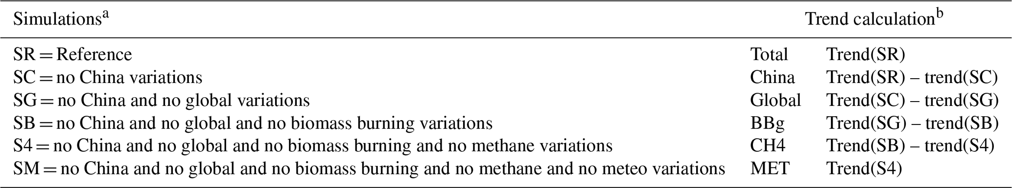
^a All the simulations are corrected from residual O₃ variations (see text). ^b The contribution of each process to the trend is calculated by dividing the corresponding trend by the total trend (TT).

Table 3 summarises the O₃ trends derived from IASI and INCA for different partial columns and for the different regions reported in Fig. 1. We choose the most populated Chinese areas where significant pollutant reductions have occurred since 2013 (Zheng et al., 2018), such as CEC – including BTH and YRD – and PRD and SCB. We also consider the KJ region as a region influenced by the pollution export from China. We made the trend values bold in the table when both IASI and INCA have trends with p < 0.05 and when the trends agree within 40 % between the model and the observations. The trend values corresponding to p < 0.05 and a poorer agreement are italicised. The CEC region shows the best agreement between the trends derived from IASI and INCA for all the columns, except the upper tropospheric columns (9–12 km). The anomalies and calculated linear trends are shown in detail on Fig. 4b, d, f and h. For this region, where both the observations and the model are the most reliable, trends are in very good agreement (< 15 %) for the 0–3, 3–6, and 6–9 km columns. Trends derived from IASI for the UT-LMS columns (9–12 km) are very small, with large p values for all the regions (Table 3). It is then difficult to compare and conclude for the upper tropospheric columns as the trends calculated from the model are mainly negative, with p < 0.05. For the PRD and the SCB, the model and the observations are less reliable for different reasons explained in Sect. 3. This leads to a poor agreement of the derived trends and a lack of reliability of the trends for these two regions (large uncertainties in the trend values; Table 3). For the BTH and YRD, included in the CEC, and for the KJ, the trends calculated from the observations and the model are in good agreement for the 3–6 and 6–9 km columns, with p < 0.01.

5 Discussion

5.1 Evaluation of the processes contributing to the trends

In this work focused on China and the period of 2008–2017, both IASI observations and INCA simulations show negative O₃ trends of similar magnitude in the lower (3–6 km) and upper (6–9 km) free troposphere in large parts of China and its downwind region. Dufour et al. (2018) suggest that negative O₃ trends derived from IASI in the lower troposphere over the North China Plain for a slightly shorter time period can be explained for almost half by NO_x emissions reduction that has been occurring in China since 2013. They argue the negative impact on the trend of these reductions compared to the positive one at the surface is due to changes in the chemical regime with the altitude. To go further on this and quantify the processes contributing to the O₃ trends, we performed several simulations with the INCA model. The objective is to remove, one by one, the interannual variability and trend induced by the different processes (emissions and meteorology). The different simulations are summarised in Table 4. First, anthropogenic emissions in China are kept constant to their 2007 values during the 2008–2017 period. Then, in addition, the global anthropogenic emissions for the rest of the world are kept constant to their 2007 values, the biomass burning emissions, and then the methane concentrations. Finally, winds used for nudging and sea surface temperatures are maintained at their 2007 values. Since the INCA model is a GCM, this method reduces considerably the interannual variability associated with meteorology. However, the meteorology is not identical from 1 year to another in the GCM. This leads to a residual trend as shown in Fig. B1 (Appendix B) for the different partial columns. This residual trend is mainly negative and small. To remove this residual trend from the model results, we subtract the meteorological variability (MET) simulation to the other simulations day by day and grid cell by grid cell. The trends derived from the initial simulation corrected from the residual ozone variations are slightly increased compared to the trends derived from the initial simulation, but they remain fully consistent, especially when p < 0.05. Then, we calculate the trend and contribution of each process as described in Table 4.

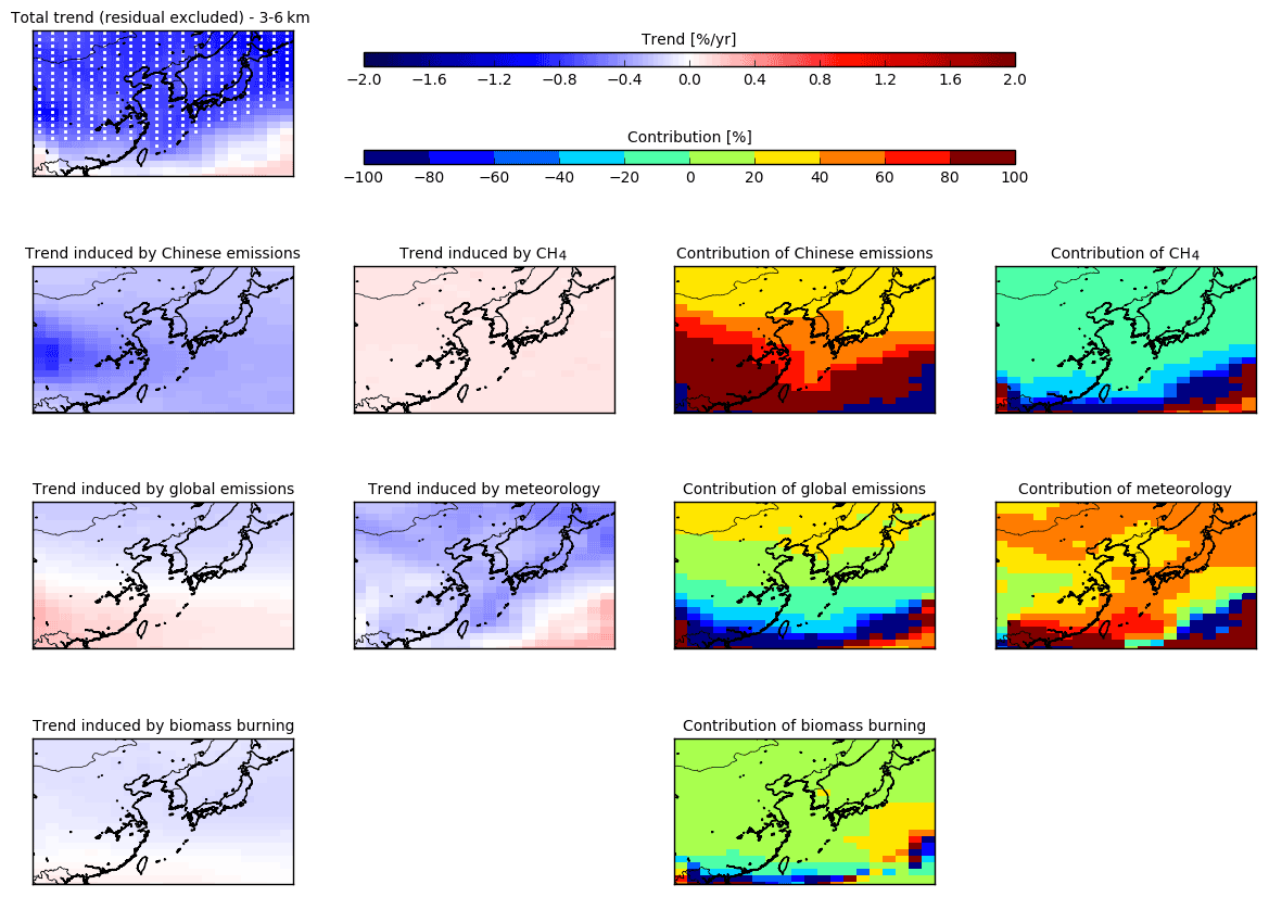
Figure 6 Trends and contributions of the meteorological variability, the Chinese anthropogenic emissions, the global anthropogenic emissions, the global biomass burning emissions, and the CH₄ to the trends calculated for the 3–6 km (see Table 4 for details on the simulations).

Table 5 Contributions (in percent) of the meteorological variability (MET), the Chinese anthropogenic emissions (China), the global anthropogenic emissions (Global), the global biomass burning emissions (BBg), and the CH₄ to the trends calculated for the 3–6 and 6–9 km partial columns for each individual region in Fig. 1.

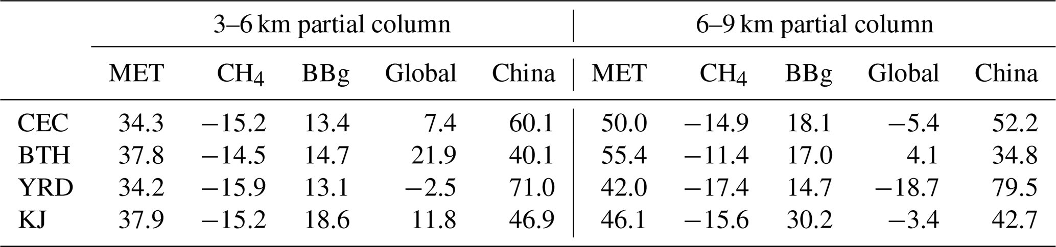
The contribution of the different processes is shown in Fig. 6 for the 3–6 km columns and in Fig. B2 for the 6–9 km columns. We focus on these two columns as they correspond to the tropospheric regions where IASI is the most sensitive and then where agreement with the model is the best. We also focus mainly on China where the p values of the total trend are smaller than 0.05. In the lower free troposphere, the main contributions to the trends are the local Chinese emissions and the meteorology, with contributions larger than 20 %. The other tested variables (global emissions, biomass burning emissions, and methane) contribute to the trends within 20 % over mainland China, with a negative contribution of methane for the entire domain. This means that the increase in methane concentrations and then the associated ozone production counteracts the ozone reduction due to the other processes (emissions and meteorology). In the upper free troposphere, meteorology and Chinese emissions also dominate the contributions. Biomass burning emissions also play a more important role in explaining the trend in the North China Plain between the Beijing region and the Yangtze River. In the south of the domain, where the robustness of the trends might be discussed as p values are larger than 0.05, strong compensations seem to operate between the contributions of the different processes, leading to a less robust assessment of their respective contributions. The different contributions for the regions where the model and the observations are the most reliable are detailed in Table 5. Chinese emissions contribute to 60 % in the main source region, the CEC, with variations inside the regions for the 3–6 km column; the Chinese emissions contribute to 40 % in BTH and more than 70 % in YRD. The Chinese contribution to the trends in the export region (KJ) remains high, with 47 % contribution. The meteorological contribution ranges from 34 % to 38 %. Methane and biomass burning emissions contributions are rather stable over the different regions around −15 % and +14 %, respectively, with the biomass burning contribution being slightly higher in the export region (19 % for KJ). Surprisingly, the global emissions contribute the most to the trends in the highly polluted region of the BTH (22 %). For the 6–9 km column, the meteorological contribution to the trends increases (about 50 % or larger) as the Chinese emissions contribution decreases. The biomass burning contribution is globally larger, especially in the export region where it reaches 30 %. The global anthropogenic emissions contribution remains small in absolute value, except in the YRD region where it becomes negative and reaches −20 %. The prevailing contribution of Chinese emissions changes in the negative O₃ trends in the lower and upper free troposphere seems to confirm the previous outcomes of Dufour et al. (2018).

5.2 Limitation of the study

The results presented in our study are not fully in line with the recent TOAR (Gaudel et al., 2018) and related works (Cooper et al., 2020; Gaudel et al., 2020), which state a general increase in tropospheric ozone during the last few decades. If negative trends are observed at the surface in developed countries, for example, in summer, positive trends for the free troposphere are reported using mainly IAGOS as a reference (Cooper et al., 2020). It is worth noting that this study brings another angle to the question of ozone changes with time over China than previously discussed during Phase I of TOAR. In the TOAR effort, our IASI product was used to describe the seasonal variability in ozone for the time period of 2010–2014 over China. However, this product was not used to assess ozone trends. Compared to the other IASI products, our product is more sensitive to the lower part of the troposphere (see Table 2 in Gaudel et al., 2018). We hope this study can bring more information to fuel the discussion on the discrepancies between the UV and IR techniques. Even if our study seems to show consistent trends derived by IASI and the model in the free troposphere, we stress, in this subsection, vigilant points for the interpretation of the results.

Length of the period

In this study, we derived trends over a limited 10-year period. Calculating short-term trends leads to an increased sensitivity to the inter- and intra-annual variations, the length of the period, and to the starting and ending point of the time series. Due to the availability of the satellite measurements and the simulated period with the model, it was not possible to extend the time period further. We tested the impact of the starting and ending point of the time series by removing 1 and 2 years at the beginning and at the end of the period. The trends derived from IASI and INCA for the 3–6 km column in the CEC for the different periods are summarised in Table B1 (Appendix B). They remain consistent with the trend derived for 2008–2017, respectively for IASI and INCA, and are within its confidence interval. These results corroborate the consistency between the modelled and observed trends and their robustness. However, it is worth noting that the calculated trends seem more sensitive to the end of the period, corresponding to a strong El Niño period, than to the beginning of the period. Removing the last 2 years of the period leads to a decrease in the IASI trend and to an increase in the INCA trend. This apparent inconsistency, which should be evaluated when longer simulations with consistent emissions and longer observation time series will be available, stresses the difficulty of working with short-term trends and the need for caution to prevent overinterpreting the results. It is worth noting that using the Theil–Sen estimator to calculate the trends changes only slightly the trends.

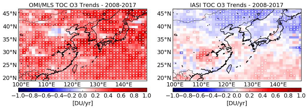
Figure 7 O₃ trends derived for the tropospheric O₃ column (TOC) from OMI/MLS and IASI for 2008–2017 at 1^∘ × 1^∘ resolution. The TOC is calculated using the same tropopause height for OMI/MLS and IASI. White crosses indicate associated p values smaller than 0.05.

Discrepancies between different satellite sounders and products

The TOAR points toward the following major discrepancy between the different satellite ozone products available for the report: the OMI UV sounder showing mainly positive trends over 2008–2016 and the IASI IR sounder showing mainly negative trends over the same period (Fig. B3; Appendix B). Over northeastern Asia, the discrepancy in the sign of the trend calculated from the different satellite products is contrasted more. The OMI/MLS and OMI-RAL products still show positive trends as all over the globe. The IASI-SOFRID (SOftware for a Fast Retrieval of IASI Data) product shows positive trends all over China, and the IASI-FORLI (Fast Optimal Retrieval on Layers for IASI) product positive trends only in the southeastern part of China. The IASI O₃ product used in this study was not included in the comparison as it is not a global product. It is worth noting that, for the TOAR, the tropospheric columns derived from the different satellite products were not based on the same tropopause height definition, and each product was considered with its native sampling. This might contribute partly to the differences between the trends, in addition to the fundamental differences in the measurement techniques (UV and IR) and the retrieval algorithms used. Possible drifts over the time have not been systematically studied in the TOAR. Some individual studies exist, but once again, they do not allow one to draw conclusions concerning the role of the drifts in the trend discrepancies. Indeed, Boynard et al. (2018) noticed a significant negative drift in the Northern Hemisphere in the IASI-FORLI product, which is not detected in the most recent IASI-SOFRID product (Barret et al., 2020). The OMI/MLS product shows a small positive drift when compared to ozonesondes but not significant when based upon a difference t test (Ziemke et al., 2019). For this study, we compare our IASI O₃ product with the OMI/MLS one. To conduct a proper comparison, we used the same definition of the tropopause height to calculate the tropospheric columns. As the OMI/MLS product provides directly tropospheric columns without ozone profiles, we selected the tropopause height used for OMI/MLS, derived from the NCEP re-analyses, as the reference tropopause height. We calculated the tropospheric columns from the IASI O₃ profiles retrieved up to the defined tropopause height. We calculated the monthly time series at the resolution of 1^∘ × 1^∘. Only the days for which IASI and OMI/MLS are both available in the considered grid cell are used to calculate the monthly means and anomalies for the given grid cell. The derived trends are shown in Fig. 7. OMI/MLS shows large positive trends all over the domain, except in the southern part of the BTH region. On its side, IASI shows trends close to zero, with positive trends over central China, the East China Sea and over the Pacific in the southeastern part of the domain, and negative trends over northern China and the Korean Peninsula. The TOC trends derived from IASI show completely different spatial patterns from the trends derived in the free troposphere (Fig. 5) and seem to reflect more the trends of UTLS column (9–12 km). Work is still needed to understand the differences in the trends derived from different satellite instruments. One especially important question is to identify from which part of the troposphere the TOC is the most representative in the different products and how the vertical sensitivity of the different instruments and retrieval algorithms influence the calculated columns and trends. Answering this question is one of the objectives of the satellite working group of the TOAR phase II, which started in 2021.

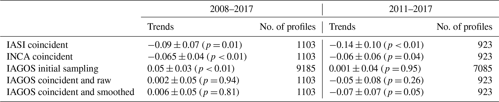
Table 6 Trends calculated for the 3–6 km O₃ columns in Europe using a subset of coincidence profiles of IASI, IAGOS, and INCA (see the text for the details on the coincidence criteria) and using the initial set of IAGOS profiles. The IAGOS trends for the coincident set of profiles are calculated from the raw and the smoothed profiles. The trends are calculated for two periods (2008–2017 and 2011–2017).

Impact of the sampling: comparison with IAGOS

The IAGOS observations are considered as a reference for free tropospheric ozone trends in the TOAR framework. Then, we try to evaluate the IASI and INCA trends using IAGOS in addition to its use for validation reported in Sect. 3. As already mentioned for the validation of IASI using IAGOS, the comparison is somehow difficult due to the limited top altitude of IAGOS profiles to properly apply the AKs to the profiles. We limit our comparison to the 3–6 km columns and explore the impact of the sampling on trend calculations. We use the same coincidence criteria as the one used in Sect. 3 to select pairs of IAGOS and IASI profiles. Based on the selected profiles, we consider the daily simulated profiles of INCA for the same day and the grids cells of the model corresponding to the latitudes and longitudes of the profiles. Partial columns are then calculated for the subset of observed and modelled profiles, and the trends are derived from the monthly anomalies. As mentioned in Sect. 3, the number of IAGOS profiles in the Chinese region is not very high (about 1000) and reduces to 315 profiles in coincidence with IASI with 213 profiles covering the pressure range from 1000 to 500 hPa. This number even falls to 26 profiles for profiles within 1000 and 250 hPa. The trends that can be calculated from this set of profiles are then not robust enough to draw conclusions. Then, we consider the European region for which more profiles are available. There are 9185 IAGOS profiles initially available for 2008–2017, with almost no measurements in 2010. Looking for the subset of profiles in coincidence with IASI strongly reduces the number of available profiles, and 3276 are selected. We consider IAGOS profiles covering the 1000–250 hPa range for a proper comparison with IASI. This allows one to reduce the proportion of a priori information potentially introduced in the IAGOS profiles when they are completed up to 60 km and smoothed by the AKs (see Sect. 3 for details). This further reduces the subset of profiles to 1103 profiles. Table 6 provides the trends derived from this subset of profiles over Europe for IASI, INCA, and IAGOS. IAGOS trends are calculated from both raw and smoothed profiles. We also provide the IAGOS trends calculated from the initial set of IAGOS profiles to evaluate the sampling impact. We calculate the trends for 2008–2017 and 2011–2017, as 2010 was not sampled by IAGOS, and the period 2008–2009 was associated to a negative anomaly (Cooper et al., 2020), which might perturb the short-term trend calculation. It is interesting to note that the difference in the sampling between the initial set of IAGOS profiles and the set in coincidence with IASI changes the calculated trends from a positive trend (0.05 DU yr⁻¹; p < 0.01) to a trend close to zero for both the raw and smoothed IAGOS columns (0.002 DU yr⁻¹ and p = 0.94; 0.006 DU yr⁻¹ and p = 0.81) for 2008–2017. For comparison, the IASI and INCA trends are negative (−0.09 DU yr⁻¹ and p = 0.01; −0.065 DU yr⁻¹ and p = 0.81) for the same period. For 2011–2017, no trend is reported from the initial set of IAGOS columns (0.001 DU yr⁻¹; p = 0.95). The trends turn out to be negative when considering the subset of IAGOS columns in coincidence with IASI (−0.05 DU yr⁻¹ and p = 0.26 for raw columns; −0.07 DU yr⁻¹ and p = 0.05 for smoothed columns). The IASI and INCA trends remain negative for this time period, with −0.14 DU yr⁻¹ (p < 0.01) and −0.06 DU yr⁻¹ (p = 0.04), respectively. The IASI negative trend is more than twice as large in absolute value compared to the ones derived from IAGOS and INCA. These results do not allow one to clearly conclude whether the negative trends derived from the model and IASI are realistic or not. They mainly show the strong sampling issue for trend calculation and stress the need to compare different data sets using, as far as possible, similar sampling to evaluate the derived trends. These results highlight again the difficulty in drawing firm conclusions on short-term trends derived from different data sets in addition to sampling differences.

6 Conclusions

In this study, the tropospheric ozone trends in China and export regions are investigated for 2008–2017 using the IASI O₃ observations and the LMDZ-OR-INCA model simulation, including the most recent Chinese emission inventory (Zheng et al., 2018). We focus mainly on the lower (3–6 km) and upper (6–9 km) free troposphere where the IASI observations and the model simulations are in good agreement, especially in the Central East China (CEC) region. These vertical layers also correspond to the atmospheric regions where the IASI observations are the most sensitive. In addition, the evaluation of the model, based on surface measurements and IAGOS observations, shows good performances of the model from the surface to the UT-LMS in the CEC. The O₃ trends calculated from the IASI observations and the INCA model are in very good agreement in the CEC region and subregions such as BTH (Beijing–Tianjin–Hebei) and YRD (Yangtze River Delta) included in the CEC. The observed and modelled trends in the CEC region are −0.07 ± 0.02 and −0.08 ± 0.02 DU yr⁻¹, respectively, for the lower free troposphere and −0.05 ± 0.02 and −0.06 ± 0.02 DU yr⁻¹, respectively, for the upper free troposphere. A good agreement is also observed in the region including the Korean Peninsula and Japan and corresponding to the region of pollution export from China. Based on sensitivity studies conducted with the INCA model, we quantify the contribution of the Chinese anthropogenic emissions, the global anthropogenic emissions, the global biomass burning emissions, methane, and meteorology to the ozone trends. In the CEC region, 60 % of the negative trend derived from the model in the lower free troposphere can be attributed to the Chinese anthropogenic emissions and 52 % in the upper free troposphere. The second contribution to explain the negative trend is the meteorological variability (34 % and 50 %, respectively). The background ozone produced from methane globally counteracts the decrease in ozone, with a contribution of about 15 % to the trends in the lower and upper free troposphere. The global anthropogenic emissions changes account for less than 10 % in the ozone trends and biomass burning emissions changes between 10 % and 20 %. These results suggest that the reduction in NO_x anthropogenic emissions that has occurred since 2013 in China has led to a decrease in ozone in the Chinese free troposphere, contrary to the increase in ozone at the surface. However, too few independent measurements, such as IAGOS or ozonesondes, are available in the region for the period during 2008–2017 to fully validate the decreasing trends calculated by both the IASI observations and the model. A comparison done in Europe, where more independent IAGOS measurements are available, shows that trend calculation can be strongly affected by the sampling of the considered data sets and the time period considered when analysing short-term trends. Particular caution should be taken to not overinterpret short-term trends and when comparing trends derived from different data sets with different sampling. In addition, comparisons between the trends calculated from the OMI/MLS O₃ tropospheric columns and the IASI ones, calculated using the same tropopause height and sampling, show large discrepancies, as already stated by the TOAR (Gaudel et al., 2018), and point toward a need to better understand how the differences in vertical sensitivity of the satellite observations impact the observed tropospheric columns and the derived trends.

Appendix A: IASI validation and INCA evaluation

Table A1 Ozonesonde stations used for the IASI O₃ validation. The term “N days” represents the number of measurements matching the coincidence criteria.

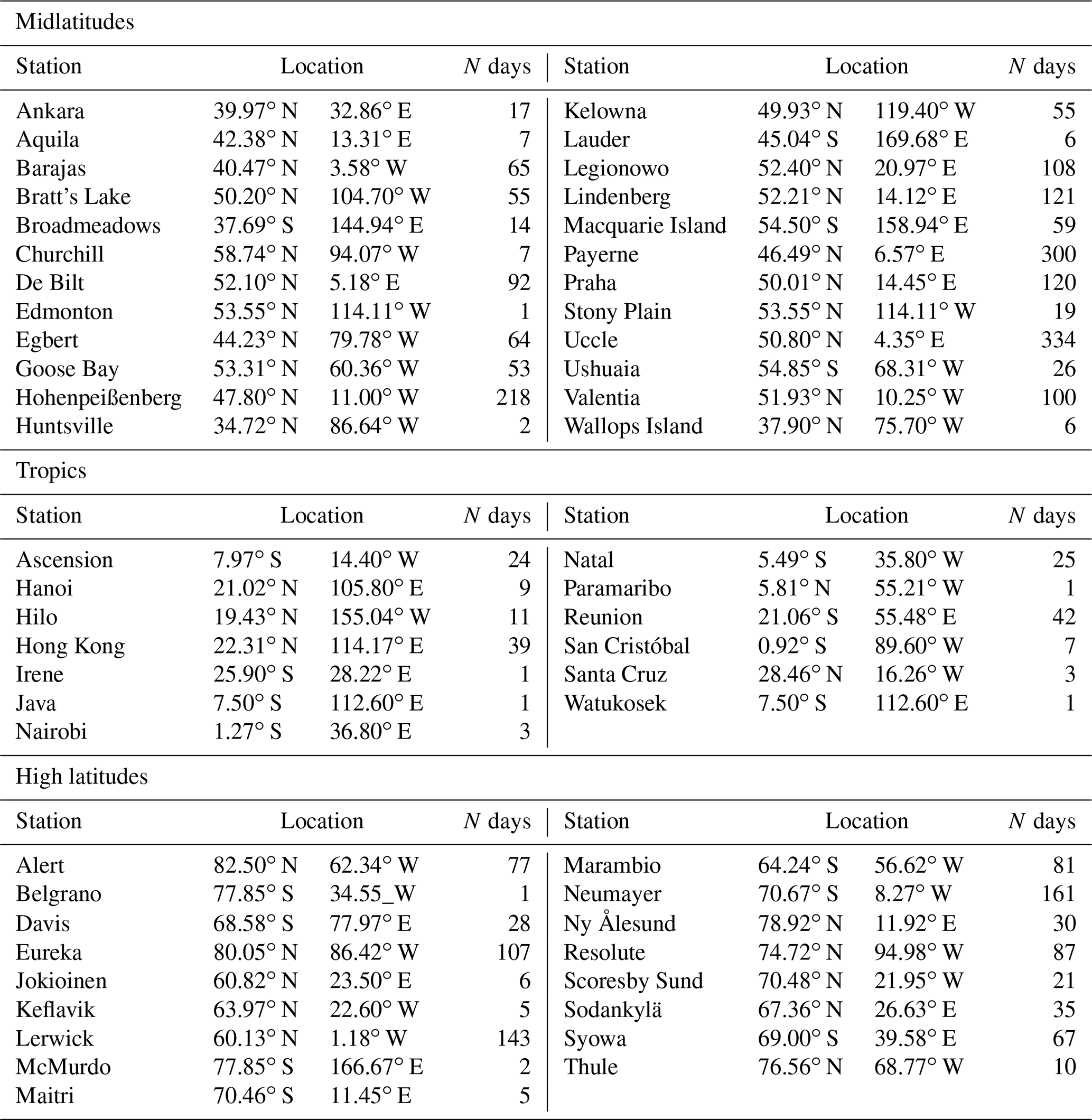
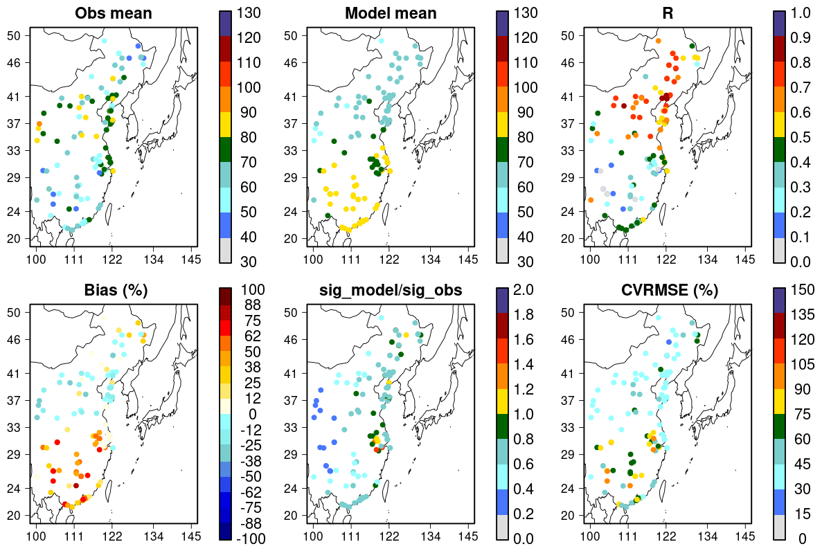
Figure A1 Mean daily O₃ concentrations (in micrograms per cubic metre) observed at the rural-type Chinese stations and simulated by INCA for 2014–2017. The statistics of the comparison at each station is shown with the correlation coefficient (R), the mean bias, the ratio of the standard deviation of the model and the observations, and the coefficient of variation of the root mean square error (CVRMSE).

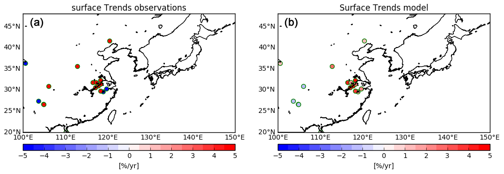
Figure A2 O₃ trends at the surface calculated from surface measurements (a) and simulations (b) for 2014–2017 at the location of rural stations described in Fig. A1. The trends is presented only when the p values are lower than 0.05.

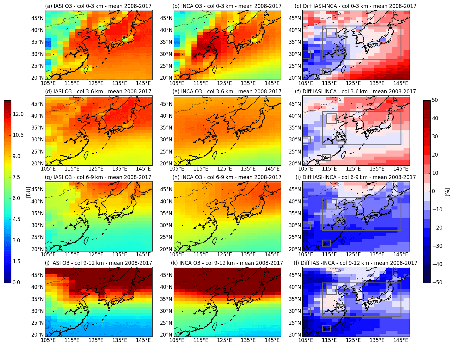
Figure A3 Mean O₃ partial columns for 2008–2017 observed with IASI (a, d, g, and j), simulated by INCA (b, e, h, and k), and their differences (c, f, i, and l). The following four different partial columns are considered: 0–3, 3–6, 6–9, and 9–12 km columns.

Appendix B: Trend analyses

Table B1 Lower free tropospheric O₃ trends (3–6 km column) calculated from IASI and INCA for the CEC for different time periods.

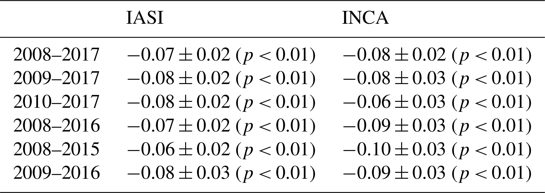
Figure B1 Residual O₃ trend derived from the INCA simulation in which all the emissions, CH₄, and meteorology are kept constant to their 2007 values. The trend is calculated for the 0–3, 3–6, 6–9, and 9–12 km O₃ partial columns.

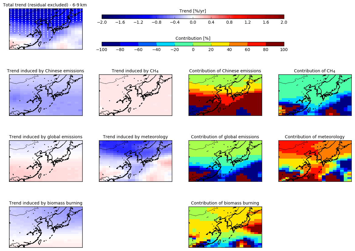
Figure B2 Trends and contributions of the meteorological variability, the Chinese anthropogenic emissions, the global anthropogenic emissions, the global biomass burning emissions, and the CH₄ to the trends calculated for the 3–6 km (see Table 4 for details on the sensitivity tests). The residual trend and its contribution is also given.

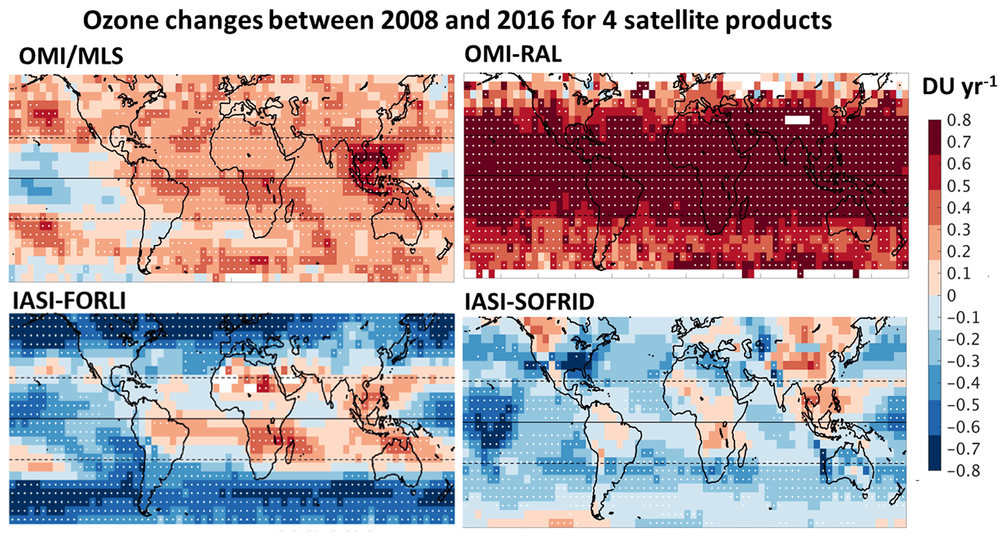
Figure B3 Global gridded ozone trends between 2008 and 2016 derived for the tropospheric columns from four satellite products (OMI/MLS, OMI-RAL, IASI-FORLI, and IASI-SOFRID) in the TOAR-I framework. The figure is an extension/update of Fig. 24 from Gaudel et al. (2018) under the CC-BY 4.0 copyright licence.