the Creative Commons Attribution 4.0 License.
the Creative Commons Attribution 4.0 License.
 | 28 Sep 2021
Evaluating consistency between total column CO2 retrievals from OCO-2 and the in situ network over North America: implications for carbon flux estimation
John B. Miller
Micheal Trudeau
Arlyn E. Andrews
Marikate Mountain
Thomas Nehrkorn
Bianca Baier
Kathryn McKain
John Mund
Kaiyu Guan
Caroline B. Alden
Feedbacks between the climate system and the carbon cycle represent a key source of uncertainty in model projections of Earth's climate, in part due to our inability to directly measure large-scale biosphere–atmosphere carbon fluxes. In situ measurements of the CO2 mole fraction from surface flasks, towers, and aircraft are used in inverse models to infer fluxes, but measurement networks remain sparse, with limited or no coverage over large parts of the planet. Satellite retrievals of total column CO2 (), such as those from NASA's Orbiting Carbon Observatory-2 (OCO-2), can potentially provide unprecedented global information about CO2 spatiotemporal variability. However, for use in inverse modeling, data need to be extremely stable, highly precise, and unbiased to distinguish abundance changes emanating from surface fluxes from those associated with variability in weather. Systematic errors in have been identified and, while bias correction algorithms are applied globally, inconsistencies persist at regional and smaller scales that may complicate or confound flux estimation. To evaluate retrievals and assess potential biases, we compare OCO-2 v10 retrievals with in situ data-constrained simulations over North America estimated using surface fluxes and boundary conditions optimized with observations that are rigorously calibrated relative to the World Meteorological Organization X2007 CO2 scale. Systematic errors in simulated atmospheric transport are independently evaluated using unassimilated aircraft and AirCore profiles. We find that the global OCO-2 v10 bias correction shifts the distribution of retrievals closer to the simulated , as intended. Comparisons between bias-corrected and simulated reveal differences that vary seasonally. Importantly, the difference between simulations and retrievals is of the same magnitude as the imprint of recent surface flux in the total column. This work demonstrates that systematic errors in OCO-2 v10 retrievals of over land can be large enough to confound reliable surface flux estimation and that further improvements in retrieval and bias correction techniques are essential. Finally, we show that independent observations, especially vertical profile data, such as those from the National Oceanic and Atmospheric Administration aircraft and AirCore programs are critical for evaluating errors in both satellite retrievals and carbon cycle models.
Please read the corrigendum first before continuing.
-
Notice on corrigendum
The requested paper has a corresponding corrigendum published. Please read the corrigendum first before downloading the article.
-
Article
(7482 KB)
- Corrigendum
-
Supplement
(15558 KB)
-
The requested paper has a corresponding corrigendum published. Please read the corrigendum first before downloading the article.
- Article
(7482 KB) - Full-text XML
- Corrigendum
-
Supplement
(15558 KB) - BibTeX
- EndNote


Interannual variability in the growth rate of atmospheric CO2 is largely driven by variability in uptake and release by terrestrial ecosystems (Heimann and Reichstein, 2008; Piao et al., 2020). Oceanic fluxes also respond to variability in climate (e.g., DeVries et al., 2019; Riebesell et al., 2009), but the amplitude of oceanic flux variability is thought to be considerably less than for terrestrial fluxes. While individual component fluxes (e.g., photosynthesis) are currently not directly measurable at scales larger than leaf or soil chambers, well-calibrated and precise measurements of CO2 have allowed us to track the accumulation of this greenhouse gas in the atmosphere and associated radiative feedbacks on the global climate, as well as its spatiotemporal variability (e.g., Tans et al., 1989). These measurements continue to provide valuable insights into surface flux processes and feedbacks (e.g., Tans et al., 1990; Ballantyne et al., 2012; Keeling et al., 2017; Arora et al., 2020). Observed spatial and temporal gradients in the CO2 mole fraction (relative to dry air) can be combined with a numerical model of atmospheric transport to infer surface fluxes (i.e., exchange of CO2 between the atmosphere and the underlying ocean or land surface), in a top-down or inverse modeling framework (e.g., Peters et al., 2007; Gurney et al., 2002). An ever-increasing global greenhouse gas measurement network and progress in modeling techniques have tremendously improved our understanding of surface processes. However, measurement networks remain sparse and continue to undersample large parts of the world, including large parts of North America, which can limit our understanding of surface flux processes in those regions. Furthermore, incompatibility across data sets that arises from inconsistent calibrations or systematic errors can significantly corrupt surface flux estimates, leading to inaccurate models of carbon–climate interactions and subsequent errors in climate forecasts.
Satellite retrievals of total column CO2 mole fraction (), such as those from NASA's Orbiting Carbon Observatory-2 (OCO-2), have the potential to provide unprecedented information about spatiotemporal patterns and variability in the Earth's atmosphere. However, space-based observations of must be extremely stable, highly precise, and free from bias to detect and quantify abundance changes caused by a change in surface fluxes (Rayner and O'Brien, 2001; Olsen, 2004; Miller et al., 2007; Houweling et al., 2004). Regional flux of terrestrial net non-fire ecosystem exchange (NEE) of CO2 can be small, as it is composed of two opposing fluxes (photosynthesis and respiration). Furthermore, NEE is ubiquitous on the terrestrial surface (unlike, for example, spatially discrete point sources from industrial emissions). Lastly, CO2 has a long lifetime in the atmosphere (and is therefore well mixed). Together, these imply that the CO2 mole fraction changes due to NEE over large regions (e.g., temperate North America) can be hard to distinguish from variability in the CO2 mole fraction resulting from flux processes and transport upwind. CO2 mole fraction changes in from NEE at the surface are diluted over the path length of the atmosphere and are largely obscured by meteorological variability (Basu et al., 2018; Feng et al., 2019).
In situ measurements that comprise global networks, such as the National Oceanic and Atmospheric Administration (NOAA)'s Global Greenhouse Reference Network (https://www.esrl.noaa.gov/gmd/ccgg/ggrn.php, last access: 20 September 2021), are rigorously evaluated and carefully calibrated relative to the World Meteorological Organization (WMO) calibration scale (data used here are reported on the X2007 scale), thus ensuring the fidelity of these measurements over timescales of seasons to decades (Andrews et al., 2014; Hall et al., 2021). The open-path nature of space-based measurements does not allow for direct calibration. Satellite retrievals require a forward model of radiative transfer that is run through an inversion system along with satellite-obtained absorption spectra of atmospheric O2 and CO2 to infer . While a great amount of progress has been made to identify and eliminate sources of uncertainty emanating from this chain of processes, e.g., in the molecular absorption model and spectroscopy (Thompson et al., 2012; Payne et al., 2020; Hobbs et al., 2020), considerable sources of uncertainty remain. These are attributed to the presence of aerosols in the column (Connor et al., 2016), clouds and cloud shadows (Massie et al., 2021), interference of jointly retrieved parameters (Kulawik et al., 2019), surface properties, and details of the instrumentation. Connor et al. (2016) estimate that aerosol-dependant biases for retrievals over land may be as large as ∼ 2 ppm (parts per million dry air mole fraction). Moreover, sensors typically degrade over time, and limited information is available to characterize resulting time-dependent systematic errors. Post-launch data corrections are routinely performed and have generally reduced bias. For example, mean bias in land nadir relative to the Total Carbon Column Observing Network (TCCON) in the v8 product was reduced from 0.72±1.22 to 0.30±1.04 ppm (O'Dell et al., 2018), and a correction in a geolocation error resulted in a decrease in across-scene standard deviation from 1.35 ppm in v8 to 0.74 ppm in the v9 data product (Kiel et al., 2019).
Currently, satellite-derived retrievals are linked to the WMO scale most directly through a set of in situ profiles obtained over a network consisting of 26 ground-based Fourier transform infrared spectrometers that comprise the TCCON (Wunch et al., 2017). However, the TCCON itself provides remotely sensed information about , and comparison with aircraft profiles have revealed errors ∼ 1 ppm (Wunch et al., 2011). Seasonal and site-dependent biases associated with the validation of OCO-2 retrievals via TCCON have also been reported (Wunch et al., 2017). OCO-2 retrievals are additionally corrected for bias by comparing with 4D CO2 mole fraction fields from global inverse models and a small area approximation, but both methods are prone to smoothing across fine-scale variability in (O'Dell et al., 2018; Corbin et al., 2008). While bias correction generally reduces inferred surface flux uncertainty when retrievals are assimilated in atmospheric inversions (Basu et al., 2013), even small retrieval errors can lead to large errors in inferred flux (Takagi et al., 2014; Chevallier et al., 2014; Villalobos et al., 2020).
Thus, a method to routinely evaluate satellite retrievals is necessary. In this study, we propose such a method that takes advantage of the relatively dense in situ network of surface, tower-based, and vertical profile CO2 mole fraction measurements over North America and leverage an ensemble of optimized flux estimates derived using the high-resolution CarbonTracker–Lagrange CO2 inverse modeling framework (Hu et al., 2019). We demonstrate an approach for constructing that offers optimal consistency with in situ measurements of CO2 dry air mole fraction calibrated relative to the WMO X2007 scale (Hall et al., 2021). We compare our simulated retrievals with the v10 OCO-2 product, hereafter , evaluate the extent to which observed differences are consistent with rigorous uncertainties on the simulated fields, and potentially correct biases in satellite retrievals. We essentially use the CarbonTracker–Lagrange modeling framework to interpolate the existing in situ measurements to the time and location of . The in situ measurement uncertainty is generally ∼ 0.15 ppm (Andrews et al., 2014), and we have carefully accounted for uncertainty in regional boundary conditions and uncertainties in the optimized fluxes. While a single realization of the simulated atmospheric transport is used here (a limitation of the approach that we aim to address in future work by using transport ensembles), we evaluate transport uncertainty using independent vertical in situ profiles of CO2. CarbonTracker–Lagrange simulations are driven by meteorological simulations from the Weather Research Forecast model system optimized for particle dispersion modeling (Nehrkorn et al., 2010), with a resolution of 10 km over continental USA and 30 km over the rest of North America, considerably higher than global in situ informed simulations that have so far been used for OCO-2 evaluation (Kiel et al., 2019; Crowell et al., 2019; Miller and Michalak, 2020). Simulated are compared with OCO-2 v10 retrievals, both before and after global bias correction, thus providing an independent evaluation of the global bias correction over North America. In principle, differences can result from errors in the retrievals or from errors in the CarbonTracker–Lagrange modeling framework, but we show that for certain seasons these differences are unlikely to result from the latter. North America is a useful test bed for evaluating consistencies and for developing improved model simulations and retrieval bias correction strategies, given the relatively dense sampling network (compared to other regions) and that the best surface flux estimates are likely to come from approaches that combine in situ measurements and satellite retrievals (Basu et al., 2013; Fischer et al., 2017; Byrne et al., 2020). The interagency North American Carbon Program (Wofsy et al., 2002) has supported intensely focused research for nearly 2 decades and has resulted in a wealth of data sets and model-to-data fusion activities that have informed model development.
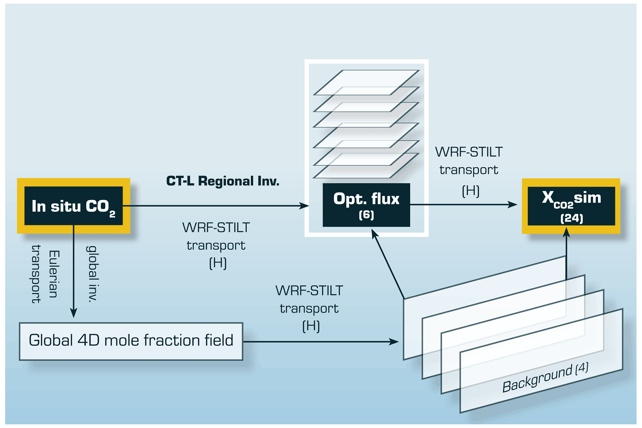
Simulated , hereafter , is constructed by estimating impact of different surface fluxes () on the total column. This involves imposing a time, latitude, longitude, and altitude-dependent lateral boundary condition or background which accounts for changes in originating outside our model domain. The chain of events that link the in situ data with the simulations is shown in Fig. 1. We use multiple ensembles of surface flux and boundary conditions to assess uncertainty in each. Comparisons with independent unassimilated aircraft and AirCore profiles are used to assess combined random and systematic errors in surface flux, background, and atmospheric transport.
2.1 Convolution method
We follow the recommended protocol for comparing satellite retrievals with modeled CO2 columns from the Atmospheric CO2 Observations from Space (ACOS) retrieval algorithm v10 (O'Dell et al., 2012).
Here, (parts per million; hereafter ppm), the total column CO2, is computed as a pressure-weighted sum of the modeled column (. ), comprising N model (i.e., not OCO-2) levels from the surface to the top of the atmosphere (0.01 hPa). is convolved with the OCO-2 averaging kernel profile (ai) and the OCO-2 prior profile () and summed according to a pressure weighting function (w; identical to h in Connor et al., 2008). w is calculated as follows:
where pi and psurf are WRF-modeled pressure at level i and at the surface, respectively. The profile sum of w is always unity. Additionally, since is reported as dry air mole fraction, WRF total pressure is converted to dry air pressure at all receptor levels.
(ppm) is constructed as follows:
Here, (ppm) represents background (i.e., lateral boundary condition; described in Sect. 2.4) and (ppm) denotes the impact of surface flux at level i of the column. is computed at discrete levels from the surface to 14 km, whereas is computed at three additional levels. These additional levels represent the upper troposphere and the stratosphere, where the influence of recent surface flux is assumed to be zero. If there are cases where recent surface fluxes influence the upper tropospheric and stratospheric air, those are accounted for as part of the background estimation. This is because models used to estimate background are also constrained by in situ measurements. Note that there may still be rare cases, e.g., in the proximity of large fires (Hooghiem et al., 2020), where surface flux influence in the upper troposphere and lower stratosphere may not be captured by this approach. is estimated as follows:
where Hi () represents the sensitivity at pressure level i of simulated to upwind surface fluxes (detailed in Sect. 2.3), and s indicates surface flux (µmol m−2 s−1). sbio denotes net ecosystem exchange (i.e., the sum of ecosystem photosynthesis and respiration), sbmb denotes biomass burning, sff corresponds to fossil fuel emissions, and socn is the net ocean–atmosphere flux. Fluxes are described in detail in Sect. 2.5.
2.2 OCO-2 retrievals and receptor selection criterion
We construct for valid land nadir and land glint from the v10 data product (Osterman et al., 2020) over North America between September 2014 and August 2015. Globally, OCO-2 retrievals are primarily obtained in three operation modes, i.e., land glint, land nadir, and ocean glint. Additionally, retrievals are obtained in target mode, for evaluation against TCCON, and a transition mode, where the sensor switches between modes. While the nadir mode is mostly used over land, over darker ocean the satellite sensor is able to receive a higher fraction of directly reflected sunlight in a separate glint mode (Eldering et al., 2017). Here, we evaluate soundings over land obtained in both the nadir and glint modes. Additionally, only retrievals that passed the aerosol and cloud-screening filers are considered (i.e., quality flagged as 0 or good).
Over North America, there can be a few thousand to tens of thousands of valid retrievals on any given day (Fig. 2a). Each retrieval covers an area of approximately 1.29 km × 2.25 km on the surface. Individual satellite retrievals are known as footprints. The satellite collects eight simultaneous footprints, and the next row of footprints are spaced 300 ms apart. For each satellite overpass (along track), we select locations every 2 s over the continental USA (i.e.,∼12 km) and 4 s (i.e.,∼24 km) over the rest of North America (Fig. 2b). These locations are usually called receptors in a Lagrangian particle dispersion model (LPDM) as they represent locations and times from which a set of particles are released and tracked back in time. In an LPDM, an ensemble of particles is released from each receptor, and the residence time of particles in the planetary boundary layer is used to calculate sensitivities describing the relationship between upwind surface fluxes and mole fraction at the receptor location. Ultimately, a library of sensitivity arrays is generated corresponding to retrieval locations. Note that these sensitivity arrays are sometimes called footprints or influence functions. Here we avoid this use of footprints so as not to create confusion with OCO-2 footprints (i.e., scenes). This method enables improved simulation of near-field transport compared to Eulerian gridded models, as particle locations are not restricted to grid boxes and meteorological fields can be interpolated to subgrid-scale locations (Lin et al., 2003), and has been used extensively in estimating regional trace gas fluxes in inverse models using in situ measurements (e.g., Schuh et al., 2009; Gourdji et al., 2012; Lauvaux et al., 2013; Alden et al., 2016; Hu et al., 2019).
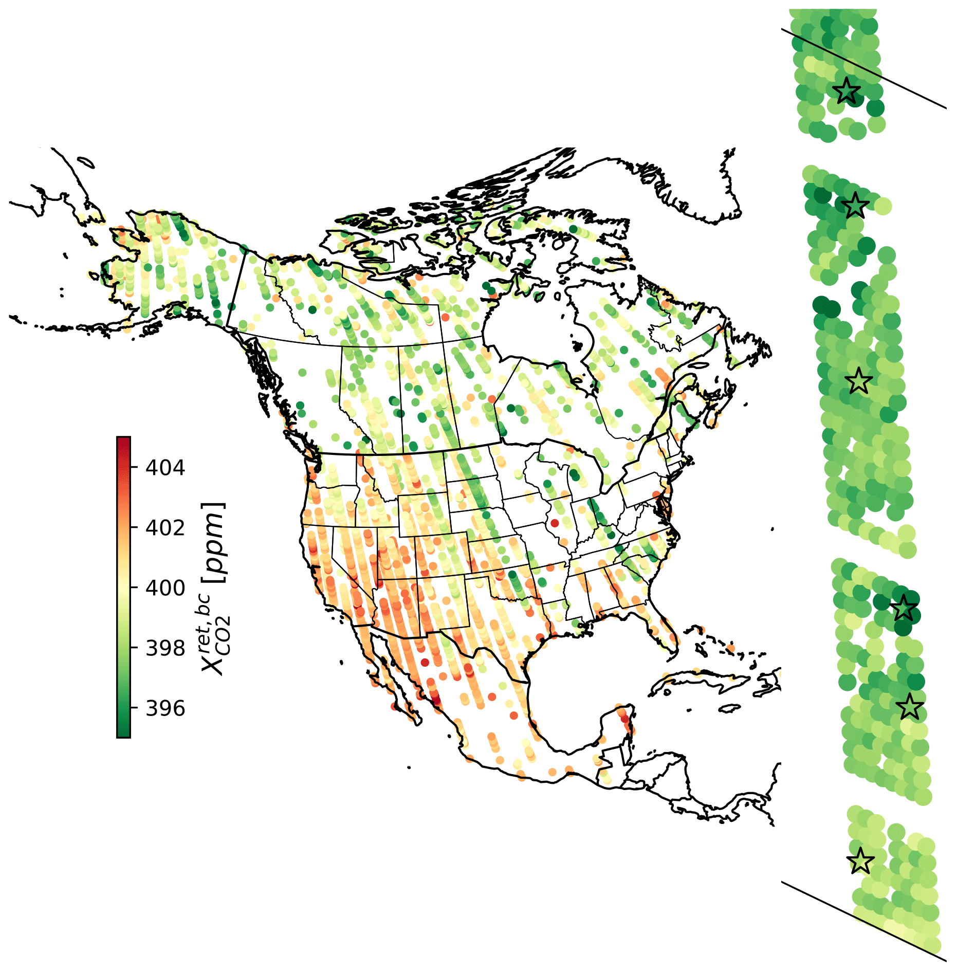
Figure 2All valid satellite retrievals for June 2015 (left). A magnified map (right) shows all retrievals for a section of an individual sounding and locations of along-track receptors (stars). Black lines in the magnified map indicate 1∘ latitude bands.
In this study, a vertical profile of receptors corresponding to a range of altitudes is created corresponding to the location of a single valid satellite retrieval. We preferentially select receptors that are in the middle of the OCO-2 track to provide the most spatially representative sample and minimize footprint-dependant biases (O'Dell et al., 2012). For this analysis, we assume that from a given receptor location is representative of all within 1 s. In total, ∼ 32 000 unique receptor profiles associated with valid retrievals are created between September 2014 and August 2015, representing ∼ 1.61 million retrievals that passed quality flags between September 2014 and August 2015. At each receptor, 24 unique are created from combinations of six flux and four background ensemble members (Fig. 1). Using an ensemble of 24 flux–background combinations provides an estimate of unresolved variability in the simulations. In this analysis, we report as the mean and standard deviation of these simulations. Similarly, represents the mean of all OCO-2 footprints within ±1 s for a selected retrieval.
A profile of receptors for each selected satellite scene consists of discrete altitude levels approximately representing the lowermost 850 hPa of the atmosphere. Models sampled for background estimation are sampled at receptor locations to account for the rest of the column (detailed in Sect. 2.4). A similar method (the application of a regional Lagrangian model to estimate source–receptor relationships) was developed recently by Wu et al. (2018). In that study, a set of model particles distributed throughout an entire column of air (weighted to appropriately represent the retrieved total column, i.e., the column receptor) was transported and tracked backward in time, and a single surface flux sensitivity array was computed for the total column. In contrast, we here establish source–receptor relationships at discrete altitude intervals and then apply appropriate vertical weighting for the column. This method has a higher computational cost and results in larger output files but adds flexibility in the simulation; for instance, a quick recalculation can be performed if the OCO-2 averaging kernel is modified, and more importantly, our simulated profiles can be used with experimental retrieval products such as partial column retrievals (e.g., Kulawik et al., 2017).
2.3 Transport model and constructing column-weighted surface sensitivity arrays: H
We use output from the Stochastic Time-Inverted Lagrangian Transport (STILT) particle dispersion model (Lin et al., 2003) driven with high-resolution meteorological fields from a customized implementation of the Weather Research and Forecasting (WRF) model (Nehrkorn et al., 2010). We use the WRF-STILT modeling configuration developed for the CarbonTracker–Lagrange modeling framework (Hu et al., 2019).
The high spatial resolution of regional models provides an appropriate framework to investigate a relatively fine-scale structure in atmospheric transport (e.g., mesoscale) and atmospheric signatures of surface flux heterogeneity. WRF model fields are computed at 10 km spatial resolution over temperate North America and 30 km spatial resolution outside of temperate North America. STILT is run offline (i.e., driven by archived hourly WRF output), and trajectories are computed backwards in time from each receptor location. STILT surface sensitivity arrays represent simulated upwind surface flux influence for 10 d prior to each observation at spatial and 1 h temporal resolution. A library of WRF-STILT surface sensitivity arrays is precomputed, archived, and can be efficiently convolved with independently estimated surface fluxes. This is in contrast to most modern Eulerian model CO2 simulations, where the transport model needs to be rerun whenever a new surface flux product becomes available. STILT surface sensitivity arrays have units of ppm (µmol m−2 s−1)−1.
The OCO-2 retrieval is a pressure-weighted mean of obtained at 20 equally spaced pressure boundaries from the surface to the top of the atmosphere. STILT receptors, however, are specified not on the pressure grid used for OCO-2 retrievals but at fixed altitudes above ground level and with high vertical resolution where strong gradients in CO2 are expected (e.g., near the surface or at the top of the planetary boundary layer). Additionally, is computed from a combination of the signal received by the spectrometer and an a priori profile (). This approach constrains the uppermost portion of the atmospheric column where the satellite sensor lacks sensitivity. The relative weights of the received signal and are described by the column averaging kernel (a; O'Dell et al., 2012), which is computed during the retrieval and archived along with and . Thus, the first step in creating column-weighted surface sensitivity arrays (H) is to interpolate and a onto the STILT grid. Then, a pressure weighting function (Eq. 2) is applied to appropriately weight the surface sensitivity obtained from all receptors for each column. The upper 150 hPa of the atmosphere is considered as part of the lateral boundary condition (the column-weighted background; Sect. 2.4), as sensitivity to recent surface flux is assumed to be zero at these pressure levels, and the WRF-STILT framework has not been optimized for upper atmospheric simulations.
2.4 Column-weighted background:
The background or lateral boundary condition is an essential component of regional models required to isolate changes in CO2 from surface fluxes within the model domain. Boundary values need to represent synoptic variability and contributions from surface fluxes outside the model domain and may contribute significantly to uncertainty in modeled (Feng et al., 2019). Here, we combine WRF-STILT back-trajectories with 4D global mole fraction fields from simulations that were optimized using global in situ measurements. From each receptor, 500 back-trajectories (simulating air parcels) are released and tracked backwards in time until the point at which they exit the WRF domain or for the duration of the simulation (10 d). At that coordinate (longitude, latitude, altitude, and time) a global 4D mole fraction field is sampled, and that value is considered as the background value for that particle. Background values for all 500 particles are then averaged to calculate the estimated background value for a given receptor. For background estimation, the WRF domain is subset to only include continental North America plus margins along the coast. These strategies minimize transport-related errors in the trajectories that inflate with increasing distance from the receptor and time of release. The background values for each receptor in a column are summed according to the pressure weighting function (Eq. 2).
Table 1Global CO2 4D mole fraction fields used in this study. Comparisons with the Global Monitoring Laboratory (GML)'s GlobalView Plus version 6.0 data product are also presented. These comparisons are provided for all assimilable observations and all assimilable observations between 4 and 8 km. For more information on the models, see the text.

In total, there are four different global 4D mole fraction fields that are informed by in situ measurements and routinely updated and sampled as background. These are two versions of CarbonTracker (CT2016 and CT2019B; Peters et al., 2007; Jacobson et al., 2020) from NOAA's Global Monitoring Laboratory (GML), the Copernicus Atmosphere Monitoring Service reanalysis (CAMS; Chevallier et al., 2019) produced by the European Centre for Medium-Range Weather Forecasts (ECMWF), and the Jena CarboScope model from the Max Planck Institute for Biogeochemistry (Rödenbeck et al., 2020). We evaluate each model against all designated assimilable CO2 data from NOAA GML's GlobalView Plus version 6.0 data product (Table 1; Schuldt et al., 2020). Assimilable data include assimilated and withheld data. Withheld data are qualitatively equivalent to assimilated data (i.e., they pass the same quality flags) but are excluded and used to evaluate model results in CarbonTracker (Andrew R. Jacobson, personal communication). Here, over 150 000 ground, tall tower, and aircraft in situ observations spanning 2014–2015 over North America and the eastern North Pacific Ocean are used. Comparisons with these observations are provided for all assimilable observations and assimilable observations between 4 and 8 km.
2.5 Surface fluxes of CO2: s
We sample optimized and imposed flux fields from regional and global inverse models. Net non-fire terrestrial ecosystem exchange (i.e., CO2 fluxes from photosynthesis and respiration from autotrophic and heterotrophic sources or sbio) are from NOAA's CarbonTracker–Lagrange (Hu et al., 2019). Briefly, CarbonTracker–Lagrange is a regional atmospheric inverse model in which biospheric fluxes for North America are optimized using surface sensitivity arrays from high-resolution WRF-STILT simulations and North American measurements of CO2 from GlobalView Plus v2.1 (Cooperative Global Atmospheric Data Integration Project, 2016), which is composed largely of data from NOAA's Global Greenhouse Gas Reference Network and from Environment and Climate Change Canada. Observations include flask air measurements from the near-surface and aircraft and quasi-continuous in situ measurements primarily made on towers. The inversions were run with three different prior estimates of sbio. These included two versions of the Carnegie–Ames–Stanford approach (CASA; Potter et al., 1993) biogeochemical model runs (CASA GFED-CMS and CASA GFEDv4.1) and the Combined Simple Biosphere/Carnegie–Ames–Stanford approach terrestrial carbon cycle model (SiBCASA; Schaefer et al., 2008). Prior error covariance parameters were derived from a maximum likelihood estimation (MLE) with fixed correlation scales of 1000 km and 7 d and also for optimized correlation scales, for each model run, resulting in six different posterior estimates of sbio. Non-biospheric fluxes include imposed biomass burning (sbmb) and fossil fuel (sff) fluxes and optimized ocean fluxes (socn) from CT2016. We use the mean of two fossil fuel emission products (Miller and ODIAC data sets) and fire emission products (GFED4.1s and GFED-CMS) used in CT2016. All fluxes are spatial and 3 h temporal resolution.
3.1 Comparing simulated and satellite retrievals
For all retrievals selected over the spatiotemporal domain of this study, the impact of the OCO-2 bias correction is 2.01±0.87 ppm, and the mean difference between seasons is 0.5 ppm (1.76 in winter and spring and 2.31 ppm in summer; blue distributions in Fig. 3). Across seasons, the difference in residuals between and is significantly lower than that between and : ppm, whereas ppm, i.e., the OCO-2 bias correction brings the distribution of OCO-2 substantially closer to the in situ data-constrained synthetic columns (), as expected. Residuals are lowest in the Northern Hemisphere summer months of June, July, and August ( ppm; Fig. 3d) and highest in the winter and spring ( ppm; Fig. 3a). Apart from the summer, mean over North America is lower than .
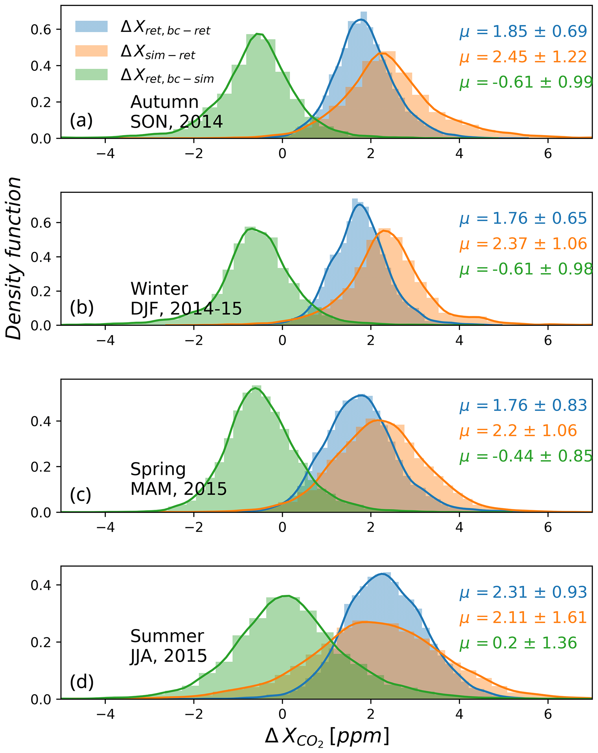
Figure 3Kernel density distributions for residuals between simulated and satellite retrievals, grouped seasonally. Blue distributions show the impact of the OCO-2 bias correction on land nadir retrievals. The orange and green curves show the difference between simulated retrievals and retrievals before and after bias correction, respectively. Printed numbers report the mean and standard deviation of residuals. Uncertainties in are discussed in Sect. 3.3.
3.2 Spatial patterns
To examine spatial patterns of simulated and retrieved soundings, we first sort retrievals in bins and then average all retrievals (and simulations) in each bin for each season. The spatial extent of OCO-2 soundings varies seasonally (Fig. 4a, e, i, m). The northern extent of valid retrievals follows the solar declination, as the OCO-2 spectrometer is unable to retrieve a signal over land that is dark or blanketed by snow. Consequently, between September and March, there are few soundings north of the USA–Canada border (∼ 49∘ N). Conversely, all of North America is observable between March and August.
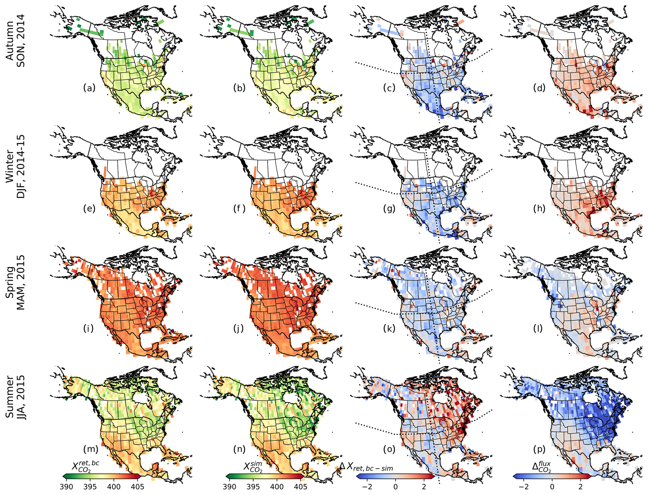
Figure 4Spatial patterns of (a, e, i, m), (b, f, j, n), and (c, g, k, o) and impact of recent surface flux ( on the (d, h, l, p) for soundings grouped seasonally and plotted on a grid. Units for all maps are in parts per million (ppm). Dotted lines in (c), (g), (k), and (o) are drawn along 40∘ N and 100∘ W.
Across seasons, and exhibit broadly similar spatial patterns (Fig. 4a–n). However, residuals between the two reveal that is usually lower than , except in the summer, when a majority of retrievals in the eastern half of the continent (right of the dotted lines in Fig. 4o) are higher than the simulations. Such coherent spatial differences are not evident when examining the mean bias over the continent (Fig. 3). Importantly, the magnitude of this difference is similar to that of the recent flux signals in the total column (Fig. 4d, h, l, p). For example, the mean residuals in the northeastern quadrant during the summer (Fig. 4o) are 0.79±1.63 ppm, significantly higher than that for the entire domain (0.09±1.38 ppm) and ∼ 45 % of the impact of recent surface flux on , i.e., .
3.3 Examining bias and uncertainty in
To establish whether differences between and presented above (Figs. 3, 4) are due to residual biases in the former, we characterize systematic errors and errors arising from unresolved variability in model fields used to construct . Cross-model standard deviations of four background models and from six biospheric flux ensembles on are shown in Fig. 5. Cross-model standard deviation in background fields is highest in the northwest during the summer (0.36 ppm) but usually less than 0.3 ppm. Over the entire spatiotemporal domain of the study, the standard deviation in estimates of and is 0.26±0.14 and 0.28±0.15 ppm, respectively. Model spread in is largest along the Pacific coast of Mexico, a region that is relatively less well constrained by the in situ network. The standard deviation in is highest in the southeastern quadrant in the summer (0.32 ppm) but usually between 0.1 and 0.3 ppm. Uncertainty from model spread in flux and background is propagated in comparisons of and presented earlier (Fig. 3).
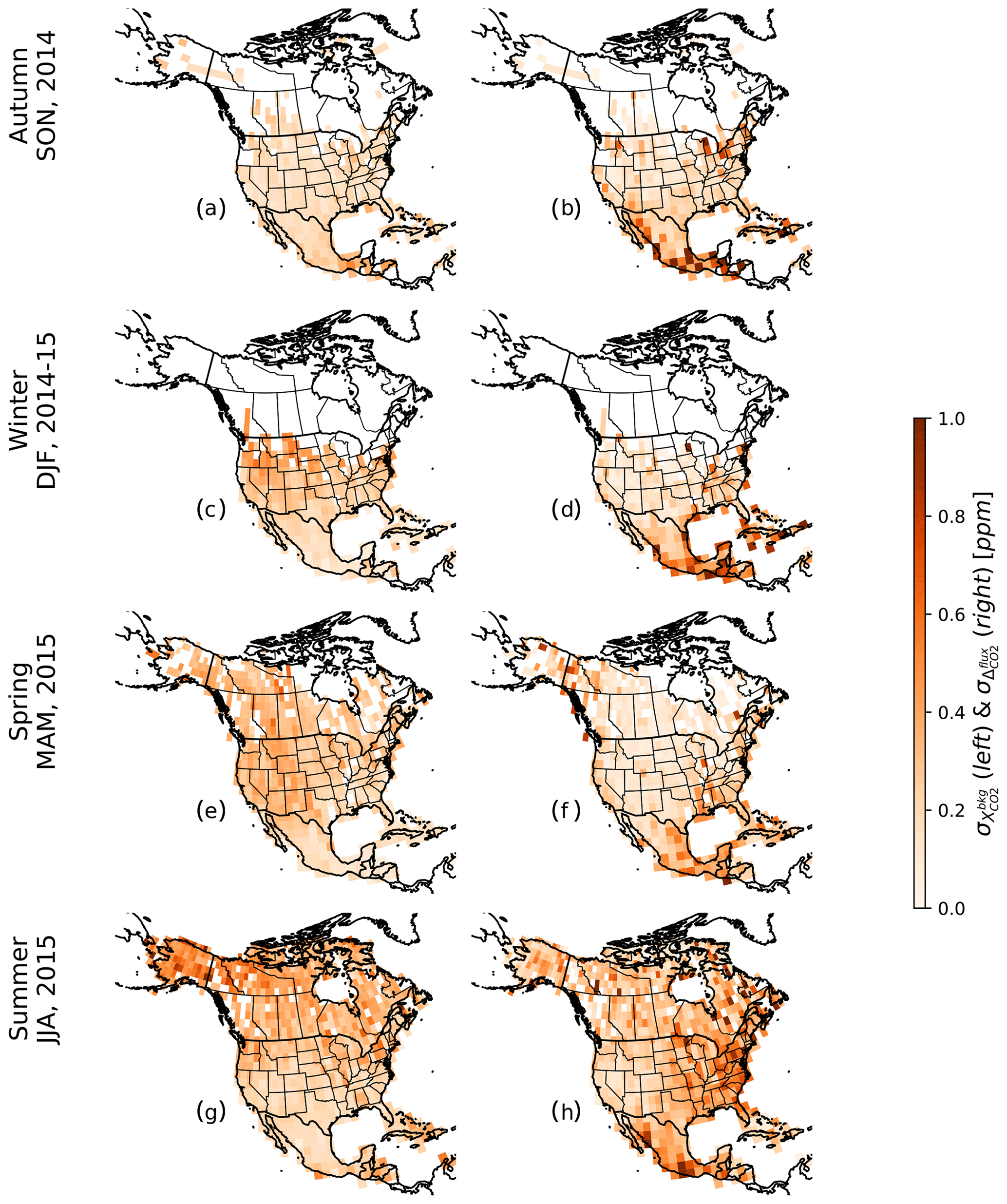
Figure 5Cross-model standard deviations flux impact (a, c, e, g) and background models (b, d, f, h). A total of six biospheric flux ensembles and four model fields for background are used in this study.
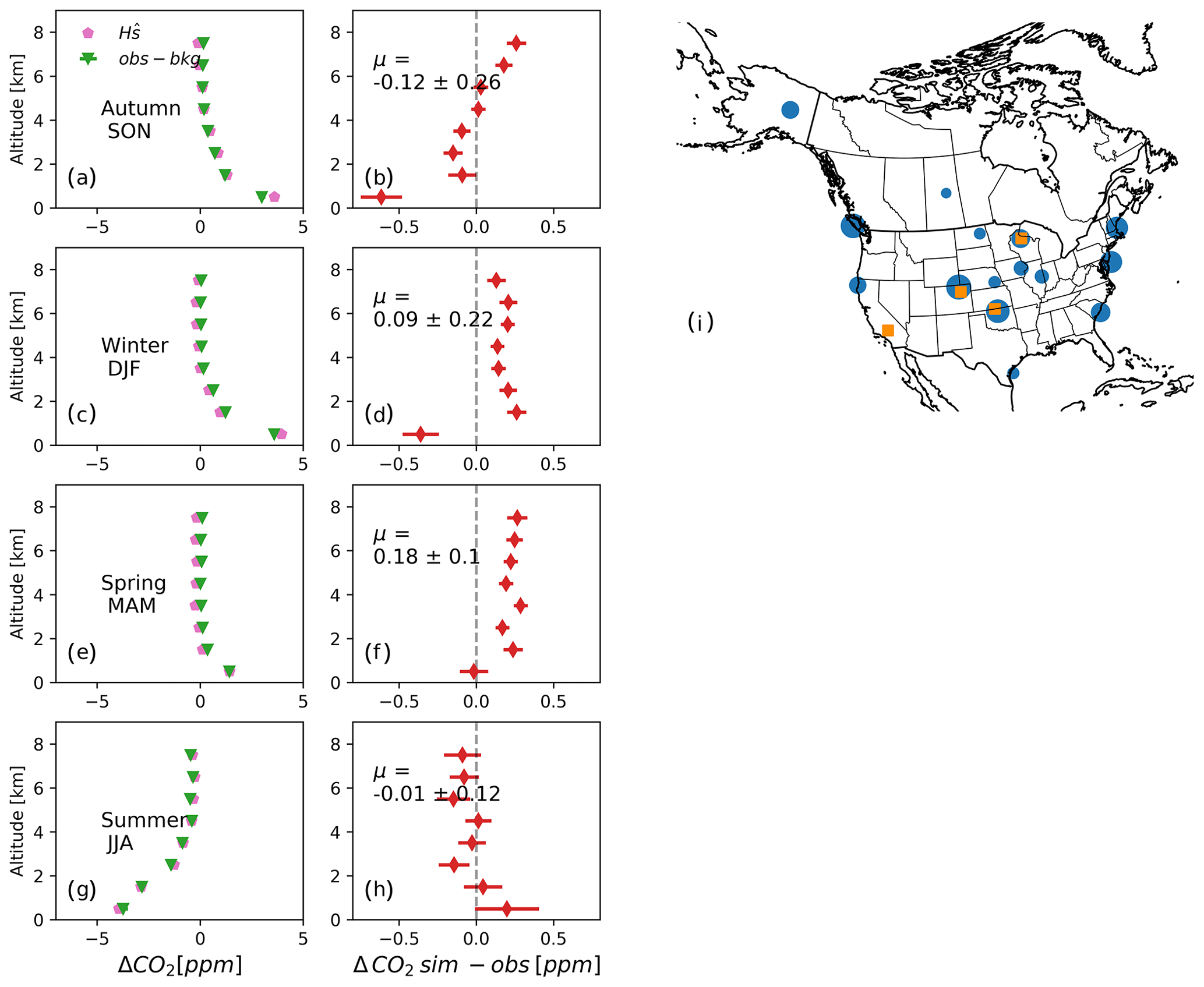
Figure 6Simulated and observed vertical profiles from independent in situ aircraft observations collected over 2007–2015 (a, c, e, g), showing simulated enhancements or depletion in CO2 as a result of surface flux (pink hexagons). Additionally, the difference between observations and CT2016 background is plotted (green triangles). We report the vertically resolved and pressure-weighted bias (mean and standard deviation) between simulations and observations (b, d, f, h). Finally, a map shows the location of aircraft profiles (blue circles in panel i) The size of each data point indicates a relative number of samples. Additionally, AirCore profile locations are also shown (orange squares in panel i). AirCore data are used to evaluate biases in boundary conditions in the upper 350 hPa of the column and are presented in Table 2.
Systematic error or bias in can arise from errors in the estimation of background and surface flux, both of which are linked by an atmospheric transport model (Fig. 1). We use the same transport model used by Hu et al. (2019) to generate source–receptor relationships and background (Sect. 2.3 and 2.4). The accuracy of the six-member ensemble of fluxes we use is also dependent upon the accuracy of WRF-STILT used in Hu et al. (2019). Thus, potential biases in WRF-STILT form a common thread for error propagation. The combined accuracy of fluxes and transport is evaluated by examining the aircraft vertical profiles of CO2 collected under NOAA GML's aircraft program (Sweeney et al., 2015) not assimilated by Hu et al. (2019). These data were obtained from NOAA GML's GlobalView Plus version 6.0 data product (Schuldt et al., 2020). We simulate all independent aircraft observations over North America for 2007–2015 (the entire spatiotemporal range of Hu et al., 2019) using existing WRF-STILT source–receptor relationships. To ensure consistency with Hu et al. (2019), we perform this evaluation with the same background conditions as in that study (i.e., CT2016). Aircraft profiles are sorted in 1 km altitude bins from the surface to 8 km a.s.l. (above sea level) and separated by season. Aircraft vertical profiles of CO2 (after removing the influence of background) and surface fluxes propagated with WRF-STILT show the net release of CO2 in non-summer months and net uptake from photosynthesis depleting near-surface CO2 during the summer (green triangles and pink hexagons in Fig. 6a, c, e, and g, respectively). The difference between independent, unassimilated observations and simulations show that bias at any given altitude level for any season is usually less than 0.5 ppm (Fig. 6b, e, h, j). Bias is also usually the largest near the surface (except in spring). The pressure-weighted partial column (from the surface to 8 km a.s.l.) mean bias (μsim − obs) ranges from −0.12 in autumn to 0.18 ppm in the spring and is comparable to the typical measurement uncertainty within the in situ Global Greenhouse Gases Research Network of ∼ 0.15 ppm as derived from long-term comparisons of differences between different within-network sampling and analysis approaches for CO2 (e.g., Andrews et al., 2014; Lan et al., 2017; Sweeney et al., 2015). Low partial column bias relative to independent vertical profile CO2 data show that errors in WRF-STILT transport contribute very minimally to bias in .
Table 2Systematic bias between global 4D CO2 fields and AirCore profiles above 8 km. Across-model mean and standard deviation is weighted with the pressure weighting function and OCO-2 averaging kernel. All values are in parts per million. The location of AirCore profiles is shown as orange squares in Fig. 6i.

To examine potential systematic errors in the highest part of the column, (above 8 km; i.e., the upper troposphere and the stratosphere), we compare 4D model fields used in this study with CO2 profiles collected by NOAA GML's AirCore program (Karion et al., 2010; Baier et al., 2021, data version v20200210). There is a considerably larger spread in the models' ability to replicate AirCore observations (Table 2) than surface and aircraft observations (Table 1 and Fig. 6). Bias between model and observations varies seasonally and is highest in the spring and lowest in the summer. However, this region forms the upper ∼ 350 hPa of the column. This has two implications. First, the contribution to total column bias reduces by ∼ 65 %. Second, the ACOS convolution equation (Eq. 1) requires that modeled estimates of be appropriately weighted with the averaging kernel (ai). ai determines the balance between information obtained by the retrieval and that contained in the OCO-2 prior (), and tends to decrease from approximately near the surface to <0.5 in the upper third of the column. Thus ∼ 50 % of the error in the highest ∼ 350 hPa of the simulated column is due to errors in . Consequently, the total contribution of model bias presented in Table 2 contributes to only ∼50 % of the bias in in the uppermost third of the column. The other source of error above 8 km is the error in , but this information is currently unavailable in the OCO-2 v10 lite files and is thus ignored in our error analysis. However, errors in are identical for and and do not affect comparisons between the two.
Combined with the standard deviation across 24 flux–background ensemble members that comprise , comparisons with independent unassimilated aircraft (Fig. 6) and AirCore profiles (Table 2) allow us to comprehensively assess uncertainties associated with . We estimate the combined uncertainty from surface flux, background estimation, and transport as follows:
where
The first two terms in Eq. (5) represent the pressure-weighted mean partial column bias between modeled and observed CO2 vertical profiles from aircraft (Fig. 6) and AirCore (Table 2), respectively. The sum of these two terms provides an estimate of bias or systematic error. The third term in Eq. (5) represents unresolved variability.
Table 3Total uncertainty estimates for , the mean difference between and , and bias in . Bias is obtained as the difference between the first two terms in the middle and left columns. All values are in parts per million. The number on the right in the third column indicates the spatial variability in bias. Finally, we also present the same quantity for the previous version of OCO-2 retrievals, i.e., the v9 data product. Note that, for v9, only land nadir retrievals are analyzed.

We find that unresolved variability due to model spread in is ∼ 0.35 ppm (second term under in Table 3), similar across seasons, and significantly lower than the uncertainty of as reported in the OCO-2 v10 lite files (∼0.6 ppm). Systematic error or bias in (first term under in Table 3) shows significant variability across seasons. Comparing this to allows an estimation of mean bias in over North America (Table 3). We find that bias ranges from −0.62 ppm in autumn to 0.14 ppm in summer. This indicates that in autumn (Figs. 3a and 4c) is entirely due to a residual bias in but almost entirely due to bias in in the spring (Figs. 3c and 4k). During summer the mean bias in is 0.05 ppm, and consequently, the mean bias in is 0.25 ppm. However, the mean conceals larger regional differences. In the northeastern quadrant, for instance, (Fig. 4o) of 0.79 ppm translates to a high bias of 0.84 ppm during the summer. Finally, we find that the OCO-2 v10 bias correction shows an improvement over the v9 bias correction, particularly in the winter.
3.4 Evaluating the OCO-2 bias correction
Bias in OCO-2 v10 is a combination of footprint bias (eight coincident across track retrievals; Cf) and feature biases (related to surface or atmospheric parameters, e.g., aerosol optical depth; Cp). Finally, a global scaling factor (C0) obtained from comparisons with TCCON retrievals is used to empirically link retrievals to the WMO scale.
To examine residual feature biases, we perform simple linear regressions between parameters used in the OCO-2 v10 bias correction with . These parameters are ΔPfrac (ppm), which accounts for fractional change in due to difference in prior and retrieved surface pressure (Kiel et al., 2019), CO2-grad del, defined as the difference of the difference between retrieved and prior CO2 at the surface and at 0.7 times the surface pressure, dws, which is the total retrieved optical depth associated with aerosols from dust, water cloud, and aerosol, and aodfine, the aerosol optical depth from sulfate and organic carbon (O'Dell et al., 2018; Osterman et al., 2020). Additionally, we perform simple linear regressions with altitude and surface albedo. All parameters are available in the OCO-2 v10 lite files. We find no significant correlations observed between and any parameters suggesting that there are no regional-scale parametric biases over North America for our study period that are not already removed by the OCO-2 global bias correction. These figures are shown in the Supplement.
The impact of recent surface flux on is small (e.g., right column in Fig. 4). The interquartile range of over the entire spatiotemporal domain is less than 1 ppm, implying that the imprint of recent surface flux on the total column is roughly half the magnitude of the OCO-2 bias correction (blue curves in Fig. 3). Moreover, only around 2 % of simulations in the summer (when surface fluxes are highest) are associated with absolute magnitudes higher than 4 ppm, indicating that recent surface flux rarely accounts for more than a ∼ 1 % change in . In autumn, is of the same magnitude as bias in (Table 3). OCO-2 retrievals in autumn 2014 are therefore unlikely to provide reliable estimates of North American surface flux. During the summer, OCO-2 has a high bias of 0.25 ppm over the continent, but this bias may be significantly larger in the eastern half of the domain (Fig. 4o). In the northeastern quadrant, for example, a potential bias of 0.84 ppm constitutes ∼ 47 % of the mean of −1.79 ppm. Considering that the vast majority of current inverse modeling or data assimilation systems used for CO2 flux estimation are designed to correct errors in an a priori estimate, the effective flux signal is considerably smaller than shown above (right column in Fig. 4). In fact, when projected onto the total column, we find that the difference between a biospheric prior flux model (CASA-CMS) and flux optimized using in situ observations over the continent by the CarbonTracker–Lagrange inversion system (using the same prior flux estimate; Hu et al., 2019) for January and July 2015 are 0.15±0.38 and 0.09±1.06 ppm, respectively. Flux adjustment impacts on are usually indistinguishable from 0 in January. While a gradient of ∼ 3 ppm is visible across the continent in July (Fig. 7), less than a third of simulated retrievals show differences between prior and optimized flux greater than ±1 ppm, when biospheric uptake over North America is strongest. Errors in terrestrial biosphere models of CO2 flux translate to similarly small impacts on , posing questions on the utility of these data in evaluating terrestrial biosphere models.
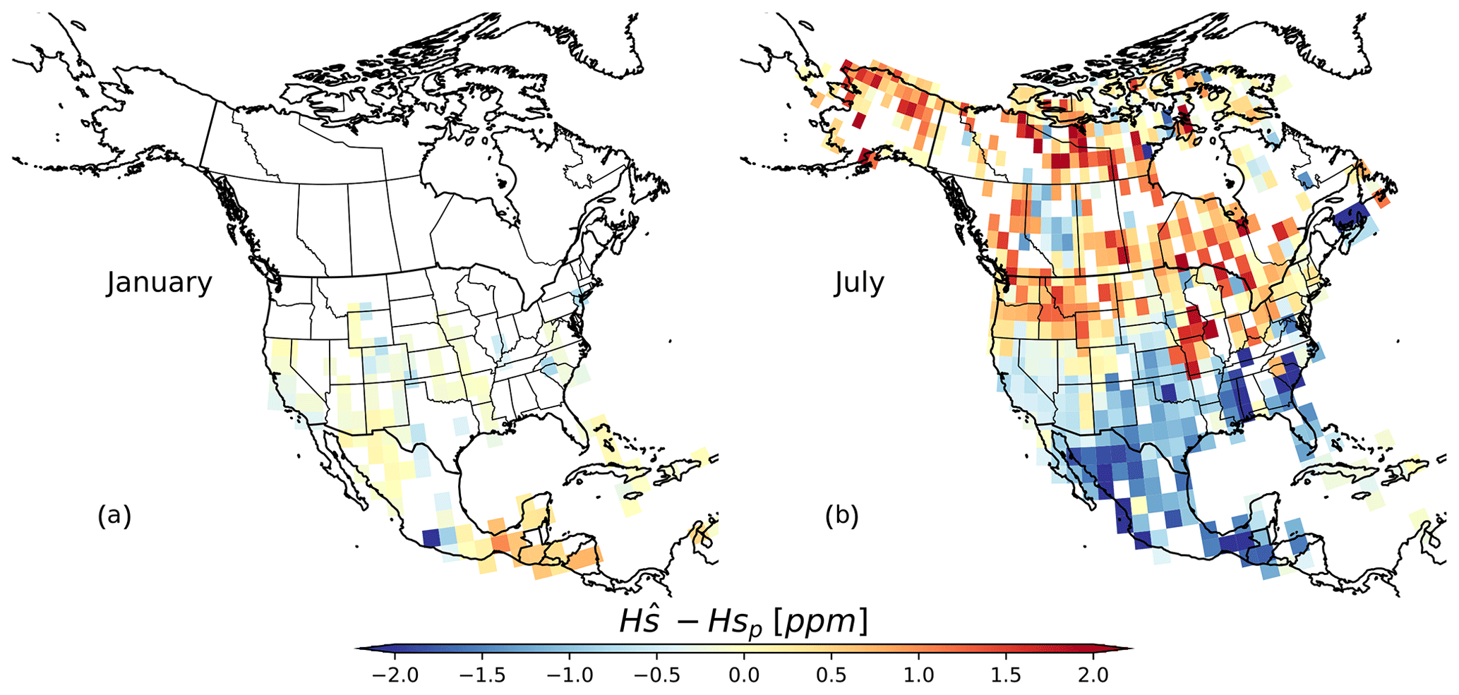
Figure 7Difference between prior and optimized biospheric flux from CarbonTracker–Lagrange shows small differences when projected onto the total column (ppm).
In this study, we compare 1 year of over North America from NASA's OCO-2 (v10; land nadir and glint retrievals) satellite against synthetic columns that are constructed using a high-resolution regional model of atmospheric transport and driven by fluxes and background that are optimally consistent with in situ measurements of CO2 dry air mole fraction, which are rigorously calibrated to the WMO CO2 X2007 scale. Although from OCO-2 and from the posterior of in situ data inversions has been compared previously, and used in its bias correction (O'Dell et al., 2018; Kiel et al., 2019), this is the first such evaluation at the regional scale that uses high-resolution atmospheric transport. We use a suite of optimized non-fire net ecosystem exchange fluxes and background fields to assess under in . Potential systematic errors in fluxes, transport, and background fields are evaluated by comparisons with vertical gradients of atmospheric CO2 from independent aircraft and AirCore vertical profiles. is associated with errors arising from unresolved variability in model fields and systematic bias. The first of these results in an uncertainty of ∼ 0.35 ppm. Bias or systematic error in is found to vary seasonally and ranges from −0.01 ppm in autumn to 0.50 ppm in the spring. Bias is highest in the upper 350 hPa of the column (Table 2), a region that is most poorly constrained by atmospheric measurements. However, the effect of this bias is relatively small in the total column comparisons.
Comparisons with show that the OCO-2 v10 global bias correction greatly improves the quality of OCO-2 data over North America (Fig. 3). However, generally good agreement between and at the continental scale masks significant differences at regional scales and for some seasons (Fig. 4). Error analysis of the components of (i.e., transport, background, and flux) allows us to better characterize the difference between simulations and retrievals. Differences in are highest in autumn and indicative of a low bias in of 0.62 ppm, which is identical to the mean impact of recent surface flux (mean over the continent is 0.64 ppm) in that season. In winter, a low bias in of 0.36 ppm is roughly 50 % of the mean of 0.71 ppm. In summer, we find spatially coherent regional patterns in . is highest in the northeastern quadrant of North America (Fig. 4o) at −0.81 ppm, 50 % of the mean expected ecosystem flux impact over this region. Since inverse models of CO2 flux usually optimize a prior flux estimate, the surface flux signal (i.e., difference between prior and optimized flux) in is minuscule (Fig. 7), significantly smaller than the magnitude of the OCO-2 v10 bias correction, and translates to extremely strenuous requirements on the quality of space-based retrievals. The OCO-2 community has worked diligently to reduce uncertainty on satellite retrievals (e.g., O'Dell et al., 2012, 2018; Kiel et al., 2019; Wunch et al., 2017; Kulawik et al., 2019); bias in v10 retrievals over North America has reduced in autumn and winter of 2014–2015 compared to the v9 data product (Table 3), but further improvement is necessary for both existing satellite data sets and planned missions that will provide this quantity in order to accurately constrain surface fluxes in a changing climate. Finally, we argue that a greatly expanded global reference network of calibrated in situ vertical profile measurements is necessary to reliably detect and correct systematic errors in satellite .
Both data and code are archived at gml.noaa.gov: https://doi.org/10.15138/cbz1-t443 (Rastogi et al., 2021). OCO-2 v10 data were obtained from NASA Goddard Earth Science Data and Information Services Center (GES DISC) (https://doi.org/10.5067/E4E140XDMPO2, OCO-2 Science Team et al., 2020). These data were produced by the OCO-2 project at the Jet Propulsion Laboratory, California Institute of Technology, and obtained from the OCO-2 data archive maintained at the NASA Goddard Earth Science Data and Information Services Center. NOAA AirCore profiles were provided by Bianca Baier and Colm Sweeney (GML, NOAA; https://doi.org/10.15138/6AV0-MY81, Baier et al., 2021, version 20200210).
The supplement related to this article is available online at: https://doi.org/10.5194/acp-21-14385-2021-supplement.
BR, JBM, AEA, CBA and KG conceived the manuscript. AEA, MT and JM made contributions to model development. LH provided biospheric surface flux ensembles, MM and TN ran WRF-STILT simulations. KM provided AirCraft observations, BB provided AirCore observations and advised on data usage. BR performed all analyses and wrote the manuscript with inputs from all co-authors.
The authors declare that they have no conflict of interest.
Publisher’s note: Copernicus Publications remains neutral with regard to jurisdictional claims in published maps and institutional affiliations.
Thanks to Sydnee Masias, for the help with the conceptual figure, and Chris O'Dell, for the comments on a previous version of this paper.
This research has been supported by the NASA CMS (Kaiyu Guan; grant no. CMS 2016), under the project “Improving the monitoring capability of carbon budget for the US Corn Belt – integrating multi-source satellite data with improved land surface modeling and atmospheric inversion to KG”, and the NASA CMS (Arlyn E. Andrews; grant no. CMS 2016), under the project “Regional Inverse Modeling in North and South America for the NASA Carbon Monitoring System to AEA”.
This paper was edited by Eliza Harris and reviewed by two anonymous referees.
Alden, C. B., Miller, J. B., Gatti, L. V., Gloor, M. M., Guan, K., Michalak, A. M., van der Laan-Luijkx, I. T., Touma, D., Andrews, A., Basso, L. S., Correia, C. S., Domingues, L. G., Joiner, J., Krol, M. C., Lyapustin, A. I., Peters, W., Shiga, Y. P., Thoning, K., van der Velde, I. R., van Leeuwen, T. T., Yadav, V., and Diffenbaugh, N. S.: Regional atmospheric CO2 inversion reveals seasonal and geographic differences in Amazon net biome exchange, Glob. Change Biol., 22, 3427–3443, https://doi.org/10.1111/gcb.13305, 2016. a
Andrews, A. E., Kofler, J. D., Trudeau, M. E., Williams, J. C., Neff, D. H., Masarie, K. A., Chao, D. Y., Kitzis, D. R., Novelli, P. C., Zhao, C. L., Dlugokencky, E. J., Lang, P. M., Crotwell, M. J., Fischer, M. L., Parker, M. J., Lee, J. T., Baumann, D. D., Desai, A. R., Stanier, C. O., De Wekker, S. F. J., Wolfe, D. E., Munger, J. W., and Tans, P. P.: CO2, CO, and CH4 measurements from tall towers in the NOAA Earth System Research Laboratory's Global Greenhouse Gas Reference Network: instrumentation, uncertainty analysis, and recommendations for future high-accuracy greenhouse gas monitoring efforts, Atmos. Meas. Tech., 7, 647–687, https://doi.org/10.5194/amt-7-647-2014, 2014. a, b, c
Arora, V. K., Katavouta, A., Williams, R. G., Jones, C. D., Brovkin, V., Friedlingstein, P., Schwinger, J., Bopp, L., Boucher, O., Cadule, P., Chamberlain, M. A., Christian, J. R., Delire, C., Fisher, R. A., Hajima, T., Ilyina, T., Joetzjer, E., Kawamiya, M., Koven, C. D., Krasting, J. P., Law, R. M., Lawrence, D. M., Lenton, A., Lindsay, K., Pongratz, J., Raddatz, T., Séférian, R., Tachiiri, K., Tjiputra, J. F., Wiltshire, A., Wu, T., and Ziehn, T.: Carbon–concentration and carbon–climate feedbacks in CMIP6 models and their comparison to CMIP5 models, Biogeosciences, 17, 4173–4222, https://doi.org/10.5194/bg-17-4173-2020, 2020. a
Baier, B., Sweeney, C., Newberger, T., Higgs, J., Wolter, S., Laboratory, and Monitoring, N. G.: NOAA AirCore atmospheric sampling system profiles, [data set], https://doi.org/10.15138/6AV0-MY81, 2021. a, b
Ballantyne, A. P., Alden, C. B., Miller, J. B., Trans, P. P., and White, J. W.: Increase in observed net carbon dioxide uptake by land and oceans during the pst 50 years, Nature, 488, 70–73, https://doi.org/10.1038/nature11299, 2012. a
Basu, S., Guerlet, S., Butz, A., Houweling, S., Hasekamp, O., Aben, I., Krummel, P., Steele, P., Langenfelds, R., Torn, M., Biraud, S., Stephens, B., Andrews, A., and Worthy, D.: Global CO2 fluxes estimated from GOSAT retrievals of total column CO2, Atmos. Chem. Phys., 13, 8695–8717, https://doi.org/10.5194/acp-13-8695-2013, 2013. a, b
Basu, S., Baker, D. F., Chevallier, F., Patra, P. K., Liu, J., and Miller, J. B.: The impact of transport model differences on CO2 surface flux estimates from OCO-2 retrievals of column average CO2, Atmos. Chem. Phys., 18, 7189–7215, https://doi.org/10.5194/acp-18-7189-2018, 2018. a
Byrne, B., Liu, J., Lee, M., Baker, I., Bowman, K. W., Deutscher, N. M., Feist, D. G., Griffith, D. W. T., Iraci, L. T., Kiel, M., Kimball, J. S., Miller, C. E., Morino, I., Parazoo, N. C., Petri, C., Roehl, C. M., Sha, M. K., Strong, K., Velazco, V. A., Wennberg, P. O., and Wunch, D.: Improved Constraints on Northern Extratropical CO2 Fluxes Obtained by Combining Surface‐Based and Space‐Based Atmospheric CO2 Measurements, J. Geophys. Res.-Atmos., 125, 29, https://doi.org/10.1029/2019JD032029, 2020. a
Chevallier, F., Palmer, P. I., Feng, L., Boesch, H., O'Dell, C. W., and Bousquet, P.: Toward robust and consistent regional CO2 flux estimates from in situ and spaceborne measurements of atmospheric CO2, Geophys. Res. Lett., 41, 1065–1070, https://doi.org/10.1002/2013GL058772, 2014. a
Chevallier, F., Remaud, M., O'Dell, C. W., Baker, D., Peylin, P., and Cozic, A.: Objective evaluation of surface- and satellite-driven carbon dioxide atmospheric inversions, Atmos. Chem. Phys., 19, 14233–14251, https://doi.org/10.5194/acp-19-14233-2019, 2019. a
Connor, B., Bösch, H., McDuffie, J., Taylor, T., Fu, D., Frankenberg, C., O'Dell, C., Payne, V. H., Gunson, M., Pollock, R., Hobbs, J., Oyafuso, F., and Jiang, Y.: Quantification of uncertainties in OCO-2 measurements of XCO2: simulations and linear error analysis, Atmos. Meas. Tech., 9, 5227–5238, https://doi.org/10.5194/amt-9-5227-2016, 2016. a, b
Connor, B. J., Boesch, H., Toon, G., Sen, B., Miller, C., and Crisp, D.: Orbiting Carbon Observatory: Inverse method and prospective error analysis, J. Geophys. Res.-Atmos., 113, 1–14, https://doi.org/10.1029/2006JD008336, 2008. a
Cooperative Global Atmospheric Data Integration Project: Multi-laboratory compilation of atmospheric carbon dioxide data for the period 1957–2015; obspack_co2_1_GLOBALVIEWplus_v2.1_2016-09-02, https://doi.org/10.15138/G3059Z, 2016. a
Corbin, K. D., Denning, A. S., Lu, L., Wang, J.-W., and Baker, I. T.: Possible representation errors in inversions of satellite CO2 retrievals, J. Geophys. Res., 113, D02301, https://doi.org/10.1029/2007JD008716, 2008. a
Crowell, S., Baker, D., Schuh, A., Basu, S., Jacobson, A. R., Chevallier, F., Liu, J., Deng, F., Feng, L., McKain, K., Chatterjee, A., Miller, J. B., Stephens, B. B., Eldering, A., Crisp, D., Schimel, D., Nassar, R., O'Dell, C. W., Oda, T., Sweeney, C., Palmer, P. I., and Jones, D. B. A.: The 2015–2016 carbon cycle as seen from OCO-2 and the global in situ network, Atmos. Chem. Phys., 19, 9797–9831, https://doi.org/10.5194/acp-19-9797-2019, 2019. a
DeVries, T., Le Quéré, C., Andrews, O., Berthet, S., Hauck, J., Ilyina, T., Landschützer, P., Lenton, A., Lima, I. D., Nowicki, M., Schwinger, J., and Séférian, R.: Decadal trends in the ocean carbon sink, P. Natl. Acad. Sci. USA, 116, 11646–11651, https://doi.org/10.1073/pnas.1900371116, 2019. a
Eldering, A., O'Dell, C. W., Wennberg, P. O., Crisp, D., Gunson, M. R., Viatte, C., Avis, C., Braverman, A., Castano, R., Chang, A., Chapsky, L., Cheng, C., Connor, B., Dang, L., Doran, G., Fisher, B., Frankenberg, C., Fu, D., Granat, R., Hobbs, J., Lee, R. A. M., Mandrake, L., McDuffie, J., Miller, C. E., Myers, V., Natraj, V., O'Brien, D., Osterman, G. B., Oyafuso, F., Payne, V. H., Pollock, H. R., Polonsky, I., Roehl, C. M., Rosenberg, R., Schwandner, F., Smyth, M., Tang, V., Taylor, T. E., To, C., Wunch, D., and Yoshimizu, J.: The Orbiting Carbon Observatory-2: first 18 months of science data products, Atmos. Meas. Tech., 10, 549–563, https://doi.org/10.5194/amt-10-549-2017, 2017. a
Feng, S., Lauvaux, T., Davis, K. J., Keller, K., Zhou, Y., Williams, C., Schuh, A. E., Liu, J., and Baker, I.: Seasonal Characteristics of Model Uncertainties From Biogenic Fluxes, Transport, and Large-Scale Boundary Inflow in Atmospheric CO2 Simulations Over North America, J. Geophys. Res.-Atmos., 124, 14325–14346, https://doi.org/10.1029/2019JD031165, 2019. a, b
Fischer, M. L., Parazoo, N., Brophy, K., Cui, X., Jeong, S., Liu, J., Keeling, R., Taylor, T. E., Gurney, K., Oda, T., and Graven, H.: Simulating estimation of California fossil fuel and biosphere carbon dioxide exchanges combining in situ tower and satellite column observations, J. Geophys. Res., 122, 3653–3671, https://doi.org/10.1002/2016JD025617, 2017. a
Gourdji, S. M., Mueller, K. L., Yadav, V., Huntzinger, D. N., Andrews, A. E., Trudeau, M., Petron, G., Nehrkorn, T., Eluszkiewicz, J., Henderson, J., Wen, D., Lin, J., Fischer, M., Sweeney, C., and Michalak, A. M.: North American CO2 exchange: inter-comparison of modeled estimates with results from a fine-scale atmospheric inversion, Biogeosciences, 9, 457–475, https://doi.org/10.5194/bg-9-457-2012, 2012. a
Gurney, K. R., Law, R. M., Denning, A. S., Rayner, P. J., Baker, D., Bousquet, P., Bruhwiler, L., Chen, Y. H., Ciais, P., Fan, S., Fung, I. Y., Gloor, M., Heimann, M., Higuchi, K., John, J., Maki, T., Maksyutov, S., Masarie, K., Peylin, P., Prather, M., Pak, B. C., Randerson, J., Sarmiento, J., Taguchi, S., Takahashi, T., and Yuen, C. W.: Towards robust regional estimates of annual mean CO2 sources and sinks, Nature, 415, 626–630, 2002. a
Hall, B. D., Crotwell, A. M., Kitzis, D. R., Mefford, T., Miller, B. R., Schibig, M. F., and Tans, P. P.: Revision of the World Meteorological Organization Global Atmosphere Watch (WMO/GAW) CO2 calibration scale, Atmos. Meas. Tech., 14, 3015–3032, https://doi.org/10.5194/amt-14-3015-2021, 2021. a, b
Heimann, M. and Reichstein, M.: Terrestrial ecosystem carbon dynamics and climate feedbacks, Nature, 451, 289–292, https://doi.org/10.1038/nature06591, 2008. a
Hobbs, J. M., Drouin, B. J., Oyafuso, F., Payne, V. H., Gunson, M. R., McDuffie, J., and Mlawer, E. J.: Spectroscopic uncertainty impacts on OCO-2/3 retrievals of XCO2, J. Quant. Spectrosc. Ra., 257, 107360, https://doi.org/10.1016/j.jqsrt.2020.107360, 2020. a
Hooghiem, J. J. D., Popa, M. E., Röckmann, T., Grooß, J.-U., Tritscher, I., Müller, R., Kivi, R., and Chen, H.: Wildfire smoke in the lower stratosphere identified by in situ CO observations, Atmos. Chem. Phys., 20, 13985–14003, https://doi.org/10.5194/acp-20-13985-2020, 2020. a
Houweling, S., Breon, F.-M., Aben, I., Rödenbeck, C., Gloor, M., Heimann, M., and Ciais, P.: Inverse modeling of CO2 sources and sinks using satellite data: a synthetic inter-comparison of measurement techniques and their performance as a function of space and time, Atmos. Chem. Phys., 4, 523–538, https://doi.org/10.5194/acp-4-523-2004, 2004. a
Hu, L., Andrews, A. E., Thoning, K. W., Sweeney, C., Miller, J. B., Michalak, A. M., Dlugokencky, E., Tans, P. P., Shiga, Y. P., Mountain, M., Nehrkorn, T., Montzka, S. A., McKain, K., Kofler, J., Trudeau, M., Michel, S. E., Biraud, S. C., Fischer, M. L., Worthy, D. E., Vaughn, B. H., White, J. W., Yadav, V., Basu, S., and Van Der Velde, I. R.: Enhanced North American carbon uptake associated with El Niño, Sci. Adv., 5, eaaw0076, https://doi.org/10.1126/sciadv.aaw0076, 2019. a, b, c, d, e, f, g, h, i, j
Jacobson, A. R., Schuldt, K. N., Miller, J. B., Oda, T., Tans, P., Andrews, A. E., Mund, J., Ott, L., Collatz, G. J., Aalto, T., Afshar, S., Aikin, K., Aoki, S., Apadula, F., Baier, B., Bergamaschi, P., Beyersdorf, A., Biraud, S. C., Bollenbacher, A., Bowling, D., Brailsford, G., Abshire, J. B., Chen, G., Chen, H., Chmura, L., Climadat, S., Colomb, A., Conil, S., Cox, A., Cristofanelli, P., Cuevas, E., Curcoll, R., Sloop, C. D., Davis, K., Wekker, S. D., Delmotte, M., DiGangi, J. P., Dlugokencky, E., Ehleringer, J., Elkins, J. W., Emmenegger, L., Fischer, M. L., Forster, G., Frumau, A., Galkowski, M., Gatti, L. V., Gloor, E., Griffis, T., Hammer, S., Haszpra, L., Hatakka, J., Heliasz, M., Hensen, A., Hermanssen, O., Hintsa, E., Holst, J., Jaffe, D., Karion, A., Kawa, S. R., Keeling, R., Keronen, P., Kolari, P., Kominkova, K., Kort, E., Krummel, P., Kubistin, D., Labuschagne, C., Langenfelds, R., Laurent, O., Laurila, T., Lauvaux, T., Law, B., Lee, J., Lehner, I., Leuenberger, M., Levin, I., Levula, J., Lin, J., Lindauer, M., Loh, Z., Lopez, M., Luijkx, I. T., Myhre, C. L., Machida, T., Mammarella, I., Manca, G., Manning, A., Manning, A., Marek, M. V., Marklund, P., Martin, M. Y., Matsueda, H., McKain, K., Meijer, H., Meinhardt, F., Miles, N., Miller, C. E., Mölder, M., Montzka, S., Moore, F., Morgui, J.-A., Morimoto, S., Munger, B., Necki, J.. Newman, S., Nichol, S., Niwa, Y., O'Doherty, S., Ottosson-Löfvenius, M., Paplawsky, B., Peischl, J., Peltola, O., Pichon, J.-M., Piper, S., Plass-Dölmer, C., Ramonet, M., Reyes-Sanchez, E., Richardson, S., Riris, H., Ryerson, T., Saito, K., Sargent, M., Sasakawa, M., Sawa, Y., Say, D., Scheeren, B., Schmidt, M., Schmidt, A., Schumacher, M., Shepson, P., Shook, M., Stanley, K., Steinbacher, M., Stephens, B., Sweeney, C., Thoning, K., Torn, M., Turnbull, J., Tørseth, K., Bulk, P. V. D., Dinther, D. V., Vermeulen, A., Viner, B., Vitkova, G., Walker, S., Weyrauch, D., Wofsy, S., Worthy, D., Young, D., and Zimnoch, M.: CarbonTracker CT2019B, NOAA Global Monitoring Laboratory, https://doi.org/10.25925/20201008, 2020. a
Karion, A., Sweeney, C., Tans, P., and Newberger, T.: AirCore: An innovative atmospheric sampling system, J. Atmos. Ocean. Tech., 27, 1839–1853, https://doi.org/10.1175/2010JTECHA1448.1, 2010. a
Keeling, R. F., Graven, H. D., Welp, L. R., Resplandy, L., Bi, J., Piper, S. C., Sun, Y., Bollenbacher, A., and Meijer, H. A. J.: Atmospheric evidence for a global secular increase in carbon isotopic discrimination of land photosynthesis, P. Natl. Acad. Sci. USA, 114, 201619240, https://doi.org/10.1073/pnas.1619240114, 2017. a
Kiel, M., O'Dell, C. W., Fisher, B., Eldering, A., Nassar, R., MacDonald, C. G., and Wennberg, P. O.: How bias correction goes wrong: measurement of X affected by erroneous surface pressure estimates, Atmos. Meas. Tech., 12, 2241–2259, https://doi.org/10.5194/amt-12-2241-2019, 2019. a, b, c, d, e
Kulawik, S. S., O'Dell, C., Payne, V. H., Kuai, L., Worden, H. M., Biraud, S. C., Sweeney, C., Stephens, B., Iraci, L. T., Yates, E. L., and Tanaka, T.: Lower-tropospheric CO2 from near-infrared ACOS-GOSAT observations, Atmos. Chem. Phys., 17, 5407–5438, https://doi.org/10.5194/acp-17-5407-2017, 2017. a
Kulawik, S. S., O'Dell, C., Nelson, R. R., and Taylor, T. E.: Validation of OCO-2 error analysis using simulated retrievals, Atmos. Meas. Tech., 12, 5317–5334, https://doi.org/10.5194/amt-12-5317-2019, 2019. a, b
Lan, X., Tans, P., Sweeney, C., Andrews, A., Jacobson, A., Crotwell, M., Dlugokencky, E., Kofler, J., Lang, P., Thoning, K., and Wolter, S.: Gradients of column CO2 across North America from the NOAA Global Greenhouse Gas Reference Network, Atmos. Chem. Phys., 17, 15151–15165, https://doi.org/10.5194/acp-17-15151-2017, 2017. a
Lauvaux, T., Ogle, S., Schuh, A. E., Andrews, A., Uliasz, M., Davis, K. J., Denning, A. S., Miles, N., Richardson, S., Lokupitiya, E., West, T. O., and Cooley, D.: Evaluating atmospheric CO2 inversions at multiple scales over a highly inventoried agricultural landscape, Glob. Change Biol., 19, 1424–1439, https://doi.org/10.1111/gcb.12141, 2013. a
Lin, J. C., Gerbig, C., Wofsy, S. C., Andrews, A. E., Daube, B. C., Davis, K. J., and Grainger, C. A.: A near-field tool for simulating the upstream influence of atmospheric observations: The Stochastic Time-Inverted Lagrangian Transport (STILT) model, J. Geophys. Res.-Atmos., 108, 4493, https://doi.org/10.1029/2002jd003161, 2003. a, b
Massie, S. T., Cronk, H., Merrelli, A., O'Dell, C., Schmidt, K. S., Chen, H., and Baker, D.: Analysis of 3D cloud effects in OCO-2 XCO2 retrievals, Atmos. Meas. Tech., 14, 1475–1499, https://doi.org/10.5194/amt-14-1475-2021, 2021. a
Miller, C. E., Crisp, D., DeCola, P. L., Olsen, S. C., Randerson, J. T., Michalak, A. M., Alkhaled, A., Rayner, P., Jacob, D. J., Suntharalingam, P., Jones, D. B., Denning, A. S., Nicholls, M. E., Doney, S. C., Pawson, S., Boesch, H., Connor, B. J., Fung, I. Y., O'Brien, D., Salawitch, R. J., Sander, S. P., Sen, B., Tans, P., Toon, G. C., Wennberg, P. O., Wofsy, S. C., Yung, Y. L., and Law, R. M.: Precision requirements for space-based XCO2 data, J. Geophys. Res.-Atmos., 112, 1–19, https://doi.org/10.1029/2006JD007659, 2007. a
Miller, S. M. and Michalak, A. M.: The impact of improved satellite retrievals on estimates of biospheric carbon balance, Atmos. Chem. Phys., 20, 323–331, https://doi.org/10.5194/acp-20-323-2020, 2020. a
Nehrkorn, T., Eluszkiewicz, J., Wofsy, S. C., Lin, J. C., Gerbig, C., Longo, M., and Freitas, S.: Coupled weather research and forecasting-stochastic time-inverted lagrangian transport (WRF-STILT) model, Meteorol. Atmos. Phys., 107, 51–64, https://doi.org/10.1007/s00703-010-0068-x, 2010. a, b
OCO-2 Science Team, Gunson, M., and Eldering, A.: OCO-2 Level 2 bias-corrected XCO2 and other select fields from the full-physics retrieval aggregated as daily files, Retrospective processing V10r, Greenbelt, MD, USA, Goddard Earth Sciences Data and Information Services Center (GES DISC) [data set], https://doi.org/10.5067/E4E140XDMPO2, 2020. a
O'Dell, C. W., Connor, B., Bösch, H., O'Brien, D., Frankenberg, C., Castano, R., Christi, M., Eldering, D., Fisher, B., Gunson, M., McDuffie, J., Miller, C. E., Natraj, V., Oyafuso, F., Polonsky, I., Smyth, M., Taylor, T., Toon, G. C., Wennberg, P. O., and Wunch, D.: The ACOS CO2 retrieval algorithm – Part 1: Description and validation against synthetic observations, Atmos. Meas. Tech., 5, 99–121, https://doi.org/10.5194/amt-5-99-2012, 2012. a, b, c, d
O'Dell, C. W., Eldering, A., Wennberg, P. O., Crisp, D., Gunson, M. R., Fisher, B., Frankenberg, C., Kiel, M., Lindqvist, H., Mandrake, L., Merrelli, A., Natraj, V., Nelson, R. R., Osterman, G. B., Payne, V. H., Taylor, T. E., Wunch, D., Drouin, B. J., Oyafuso, F., Chang, A., McDuffie, J., Smyth, M., Baker, D. F., Basu, S., Chevallier, F., Crowell, S. M. R., Feng, L., Palmer, P. I., Dubey, M., García, O. E., Griffith, D. W. T., Hase, F., Iraci, L. T., Kivi, R., Morino, I., Notholt, J., Ohyama, H., Petri, C., Roehl, C. M., Sha, M. K., Strong, K., Sussmann, R., Te, Y., Uchino, O., and Velazco, V. A.: Improved retrievals of carbon dioxide from Orbiting Carbon Observatory-2 with the version 8 ACOS algorithm, Atmos. Meas. Tech., 11, 6539–6576, https://doi.org/10.5194/amt-11-6539-2018, 2018. a, b, c, d, e
Olsen, S. C.: Differences between surface and column atmospheric CO2 and implications for carbon cycle research, J. Geophys. Res., 109, 1–11, https://doi.org/10.1029/2003jd003968, 2004. a
Osterman, G., O’Dell, C., Eldering, A., Fisher, B., Crisp, D., Cheng, C., Frankenberg, C., Lambert, A., Gunson, M. R., Mandrake, L., Wunch, D., and Kiel, M.: Orbiting Carbon Observatory-2 & 3 (OCO-2 & OCO-3): Data Product User’s Guide, Operational Level 2 Data Versions 10 and Lite File Version 10 and VEarly, NASA Jet Propulsion Laboratory, California Institute of Technology Pasadena, California, available at: https://docserver.gesdisc.eosdis.nasa.gov/public/project/OCO/OCO2_OCO3_B10_DUG.pdf (last access: 20 September 2021), 2020. a, b
Payne, V. H., Drouin, B. J., Oyafuso, F., Kuai, L., Fisher, B. M., Sung, K., Nemchick, D., Crawford, T. J., Smyth, M., Crisp, D., Adkins, E., Hodges, J. T., Long, D. A., Mlawer, E. J., Merrelli, A., Lunny, E., and O'Dell, C. W.: Absorption coefficient (ABSCO) tables for the Orbiting Carbon Observatories: Version 5.1, J. Quant. Spectrosc. Ra., 255, 107217, https://doi.org/10.1016/j.jqsrt.2020.107217, 2020. a
Peters, W., Jacobson, A. R., Sweeney, C., Andrews, A. E., Conway, T. J., Masarie, K., Miller, J. B., Bruhwiler, L. M. P., Petron, G., Hirsch, A. I., Worthy, D. E. J., van der Werf, G. R., Randerson, J. T., Wennberg, P. O., Krol, M. C., and Tans, P. P.: An atmospheric perspective on North American carbon dioxide exchange: CarbonTracker, P. Natl. Acad. Sci. USA, 104, 18925–18930, https://doi.org/10.1073/pnas.0708986104, 2007. a, b
Piao, S., Wang, X., Wang, K., Li, X., Bastos, A., Canadell, J. G., Ciais, P., Friedlingstein, P., and Sitch, S.: Interannual variation of terrestrial carbon cycle: Issues and perspectives, Glob. Change Biol., 26, 300–318, https://doi.org/10.1111/gcb.14884, 2020. a
Potter, C. S., Randerson, J. T., Field, C. B., Matson, P. A., Vitousek, P. M., Mooney, H. A., and Klooster, S. A.: Terrestrial ecosystem production: a process model based on global satellite and surface data, Global Biogeochem. Cy., 7, 811–841, 1993. a
Rastogi, B., Miller, J. B., Trudeau, M., Andrews, A., Hu, L., Mountain, M., Nehrkorn, T., Baier, B., McKain, K., Mund, J., Guan, K., and Alden, C. B.: Source code and model output for constructing synthetic OCO-2 columns and evaluation of bias, Global Monitoring Laboratory [data set], https://doi.org/10.15138/cbz1-t443, 2021. a
Rayner, P. J. and O'Brien, D. M.: The utility of remotely sensed CO2 concentration data in surface source inversions, Geophys. Res. Lett., 28, 175–178, https://doi.org/10.1029/2000GL011912, 2001. a
Riebesell, U., Rtzinger, A. K., and Oschlies, A.: Sensitivities of marine carbon fluxes to ocean change, P. Natl. Acad. Sci. USA, 106, 20602–20609, https://doi.org/10.1073/pnas.0813291106, 2009. a
Rödenbeck, C., Zaehle, S., Keeling, R., and Heimann, M.: The European carbon cycle response to heat and drought as seen from atmospheric CO2 data for 1999–2018, Philos. T. Roy. Soc. B, 375, 20190506, https://doi.org/10.1098/rstb.2019.0506, 2020. a
Schaefer, K., Collatz, G. J., Tans, P., Denning, A. S., Baker, I., Berry, J., Prihodko, L., Suits, N., and Philpott, A.: Combined simple biosphere/carnegie-ames-stanford approach terrestrial carbon cycle model, J. Geophys. Res.-Biogeo., 113, 1–13, https://doi.org/10.1029/2007JG000603, 2008. a
Schuh, A. E., Denning, A. S., Uliasz, M., and Corbin, K. D.: Seeing the forest through the trees: Recovering large-scale carbon flux biases in the midst of small-scale variability, J. Geophys. Res.-Biogeo., 114, 1–11, https://doi.org/10.1029/2008JG000842, 2009. a
Schuldt, K. N., Mund, J., Luijkx, I. T., Jacobson, A. R., Cox, A., Vermeulen, A., Manning, A., Beyersdorf, A., Manning, A., Karion, A., Hensen, A., Andrews, A., Frumau, A., Colomb, A., Scheeren, B., Law, B., Baier, B., Munger, B., Paplawsky, B., Viner, B., Stephens, B., Daube, B., Labuschagne, C., Myhre, C. L., Hanson, C., Miller, C. E., Plass-Duelmer, C., Sloop, C. D., Sweeney, C., Kubistin, D., Goto, D., Jaffe, D., Say, D., Dinther, D. V., Bowling, D., Young, D., Weyrauch, D., Worthy, D., Dlugokencky, E., Gloor, E., Cuevas, E., Reyes-Sanchez, E., Hintsa, E., Kort, E., Morgan, E., Apadula, F., Gheusi, F., Meinhardt, F., Moore, F., Vitkova, G., Chen, G., Bentz, G., Manca, G., Brailsford, G., Forster, G., Riris, H., Meijer, H., Matsueda, H., Chen, H., Levin, I., Lehner, I., Mammarella, I., Bartyzel, J., Abshire, J. B., Elkins, J. W., Levula, J., Necki, J., Pichon, J. M., Peischl, J., Müller-Williams, J., Turnbull, J., Miller, J. B., Lee, J., Lin, J., Morgui, J.-A., DiGangi, J. P., Hatakka, J., Coletta, J. D., Holst, J., Kominkova, K., McKain, K., Saito, K., Aikin, K., Davis, K., Thoning, K., Tørseth, K., Haszpra, L., Mitchell, L., Gatti, L. V., Emmenegger, L., Chmura, L., Merchant, L., Sha, M. K., Delmotte, M., Fischer, M. L., Schumacher, M., Torn, M., Leuenberger, M., Steinbacher, M., Schmidt, M., Mazière, M. D., Sargent, M., Lindauer, M., Mölder, M., Martin, M. Y., Shook, M., Galkowski, M., Heliasz, M., Marek, M. V., Ramonet, M., Zimnoch, M., Lopez, M., Mihalopoulos, N., Miles, N., Laurent, O., Peltola, O., Hermanssen, O., Trisolino, P., Cristofanelli, P., Kolari, P., Krummel, P., Shepson, P., Smith, P., Rivas, P. P., Bakwin, P., Bergamaschi, P., Keronen, P., Tans, P., Bulk, P. V. D., Keeling, R., Ramos, R., Langenfelds, R., Curcoll, R., Commane, R., Newman, S., Hammer, S., Richardson, S., Biraud, S. C., Conil, S., Clark, S., Morimoto, S., Aoki, S., O'Doherty, S., Climadat, S., Wekker, S. D., Kawa, S. R., Montzka, S., Walker, S., Piper, S., Wofsy, S., Nichol, S., Lauvaux, T., Ryerson, T., Griffis, T., Biermann, T., Machida, T., Laurila, T., Aalto, T., Gomez-Trueba, V., Joubert, W., Niwa, Y., Sawa, Y., and Loh, Z.: Multi-laboratory compilation of atmospheric carbon dioxide data for the period 1957–2019; obspack_co2_1_GLOBALVIEWplus_v6.0_2020-09-11, https://doi.org/10.25925/20200903, 2020. a, b
Sweeney, C., Karion, A., Wolter, S., Newberger, T., Guenther, D., Higgs, J. A., Andrews, A. E., Lang, P. M., Neff, D., Dlugokencky, E., Miller, J. B., Montzka, S. A., Miller, B. R., Masarie, K. A., Biraud, S. C., Novelli, P. C., Crotwell, M., Crotwell, A. M., Thoning, K., and Tans, P. P.: Seasonal climatology of CO2 across North America from aircraft measurements in the NOAA/ESRL Global Greenhouse Gas Reference Network, J. Geophys. Res.-Atmos., 120, 5155–5190, https://doi.org/10.1002/2014JD022591, 2015. a, b
Takagi, H., Houweling, S., Andres, R. J., Belikov, D., Bril, A., Boesch, H., Butz, A., Guerlet, S., Hasekamp, O., Maksyutov, S., Morino, I., Oda, T., O'Dell, C. W., Oshchepkov, S., Parker, R., Saito, M., Uchino, O., Yokota, T., Yoshida, Y., and Valsala, V.: Influence of differences in current GOSAT XCO2 retrievals on surface flux estimation, Geophys. Res. Lett., 41, 2598–2605, https://doi.org/10.1002/2013GL059174, 2014. a
Tans, P. P., Conway, T. J., and Nakazawa, T.: Latitudinal distribution of the sources and sinks of atmospheric carbon dioxide derived from surface observations and an atmospheric transport model, J. Geophys. Res., 94, 5151–5172, https://doi.org/10.1029/JD094iD04p05151, 1989. a
Tans, P. P., Fung, I. Y., and Takahashi, T.: Observational constraints on the global atmospheric CO2 budget, Science, 247, 1431–1438, https://doi.org/10.1126/science.247.4949.1431, 1990. a
Thompson, D. R., Chris Benner, D., Brown, L. R., Crisp, D., Malathy Devi, V., Jiang, Y., Natraj, V., Oyafuso, F., Sung, K., Wunch, D., Castaño, R., and Miller, C. E.: Atmospheric validation of high accuracy CO2 absorption coefficients for the OCO-2 mission, J. Quant. Spectrosc. Ra., 113, 2265–2276, https://doi.org/10.1016/j.jqsrt.2012.05.021, 2012. a
Villalobos, Y., Rayner, P., Thomas, S., and Silver, J.: The potential of Orbiting Carbon Observatory-2 data to reduce the uncertainties in CO2 surface fluxes over Australia using a variational assimilation scheme, Atmos. Chem. Phys., 20, 8473–8500, https://doi.org/10.5194/acp-20-8473-2020, 2020. a
Wofsy, S. C. and Harriss, R. C.: The North American Carbon Program (NACP), Report of the NACP Committee of the U.S. Interagency Carbon Cycle Science Program, US Global Change Research Program, Washington, DC, p. 62, 2002. a
Wu, D., Lin, J. C., Fasoli, B., Oda, T., Ye, X., Lauvaux, T., Yang, E. G., and Kort, E. A.: A Lagrangian approach towards extracting signals of urban CO2 emissions from satellite observations of atmospheric column CO2 (XCO2): X-Stochastic Time-Inverted Lagrangian Transport model (“X-STILT v1”), Geosci. Model Dev., 11, 4843–4871, https://doi.org/10.5194/gmd-11-4843-2018, 2018. a
Wunch, D., Toon, G. C., Blavier, J. F. L., Washenfelder, R. A., Notholt, J., Connor, B. J., Griffith, D. W., Sherlock, V., and Wennberg, P. O.: The total carbon column observing network, Philos. T. Roy. Soc. A, 369, 2087–2112, https://doi.org/10.1098/rsta.2010.0240, 2011. a
Wunch, D., Wennberg, P. O., Osterman, G., Fisher, B., Naylor, B., Roehl, C. M., O'Dell, C., Mandrake, L., Viatte, C., Kiel, M., Griffith, D. W. T., Deutscher, N. M., Velazco, V. A., Notholt, J., Warneke, T., Petri, C., De Maziere, M., Sha, M. K., Sussmann, R., Rettinger, M., Pollard, D., Robinson, J., Morino, I., Uchino, O., Hase, F., Blumenstock, T., Feist, D. G., Arnold, S. G., Strong, K., Mendonca, J., Kivi, R., Heikkinen, P., Iraci, L., Podolske, J., Hillyard, P. W., Kawakami, S., Dubey, M. K., Parker, H. A., Sepulveda, E., García, O. E., Te, Y., Jeseck, P., Gunson, M. R., Crisp, D., and Eldering, A.: Comparisons of the Orbiting Carbon Observatory-2 (OCO-2) XCO2 measurements with TCCON, Atmos. Meas. Tech., 10, 2209–2238, https://doi.org/10.5194/amt-10-2209-2017, 2017. a, b, c
The requested paper has a corresponding corrigendum published. Please read the corrigendum first before downloading the article.
- Article
(7482 KB) - Full-text XML
- Corrigendum
-
Supplement
(15558 KB) - BibTeX
- EndNote