the Creative Commons Attribution 4.0 License.
the Creative Commons Attribution 4.0 License.
 | 27 Sep 2021
The regional impact of urban emissions on air quality in Europe: the role of the urban canopy effects
Jan Karlický
Jana Marková
Tereza Nováková
Marina Liaskoni
Lukáš Bartík
Urban areas are hot spots of intense emissions, and they influence air quality not only locally but on a regional or even global scale. The impact of urban emissions over different scales depends on the dilution and chemical transformation of the urban plumes which are governed by the local- and regional-scale meteorological conditions. These are influenced by the presence of urbanized land surface via the so-called urban canopy meteorological forcing (UCMF). In this study, we investigate for selected central European cities (Berlin, Budapest, Munich, Prague, Vienna and Warsaw) how the urban emission impact (UEI) is modulated by the UCMF for present-day climate conditions (2015–2016) using two regional climate models, the regional climate models RegCM and Weather Research and Forecasting model coupled with Chemistry (WRF-Chem; its meteorological part), and two chemistry transport models, Comprehensive Air Quality Model with Extensions (CAMx) coupled to either RegCM and WRF and the “chemical” component of WRF-Chem. The UCMF was calculated by replacing the urbanized surface by a rural one, while the UEI was estimated by removing all anthropogenic emissions from the selected cities.
We analyzed the urban-emission-induced changes in near-surface concentrations of NO2, O3 and PM2.5. We found increases in NO2 and PM2.5 concentrations over cities by 4–6 ppbv and 4–6 µg m−3, respectively, meaning that about 40 %–60 % and 20 %–40 % of urban concentrations of NO2 and PM2.5 are caused by local emissions, and the rest is the result of emissions from the surrounding rural areas. We showed that if UCMF is included, the UEI of these pollutants is about 40 %–60 % smaller, or in other words, the urban emission impact is overestimated if urban canopy effects are not taken into account. In case of ozone, models due to UEI usually predict decreases of around −2 to −4 ppbv (about 10 %–20 %), which is again smaller if UCMF is considered (by about 60 %). We further showed that the impact on extreme (95th percentile) air pollution is much stronger, and the modulation of UEI is also larger for such situations. Finally, we evaluated the contribution of the urbanization-induced modifications of vertical eddy diffusion to the modulation of UEI and found that it alone is able to explain the modeled decrease in the urban emission impact if the effects of UCMF are considered. In summary, our results showed that the meteorological changes resulting from urbanization have to be included in regional model studies if they intend to quantify the regional footprint of urban emissions. Ignoring these meteorological changes can lead to the strong overestimation of UEI.
- Article
(22270 KB) - Full-text XML
- BibTeX
- EndNote


Already more than 50 % of the human population lives in urban areas, and an increase over 60 % during the upcoming decades is foreseen (UN, 2018). The consequences of urbanization (i.e., the transition from rural to urban surfaces) on atmospheric conditions are evident (Folberth et al., 2015), and they affect both the climate (Zhao et al., 2014; Zhu et al., 2017; Huszar et al., 2014; Karlický et al., 2018, 2020) and air pollution (Freney et al., 2014; Timothy and Lawrence, 2009; Butler and Lawrence, 2009; Im and Kanakidou, 2012; Huszar et al., 2016a), as well as the possible interactions between them (e.g., Huszar et al., 2018b, 2020a; Han et al., 2020; Fan et al., 2020) that often lead to complex counteracting effects (Yu et al., 2020).
In principle, cities influence the physical and chemical state of the atmosphere via two primary pathways. First of all, urban canopies are covered by artificial materials and objects in a specific geometric layout (building and streets) resulting in a range of effects on the meteorological conditions – i.e., they act via the so-called urban canopy meteorological forcing (UCMF) as defined by Huszar et al. (2020a). In particular, temperature is increased in cities due to the urban heat island (UHI) effect (Oke, 1982; Oke et al., 2017). Due to enhanced roughness, the city-scale wind speed is decreased (Huszar et al., 2014; Jacobson et al., 2015; Zha et al., 2019), while for turbulence (especially the vertical eddy diffusivity) a strong increase is seen (Barnes et al., 2014; Huszar et al., 2018b, 2020a; Ren et al., 2019). Secondly, due to high population density and thus concentrated human activities and energy demand, cities represent an intense source of both greenhouse (Folberth et al., 2012) and short-lived pollutants that impact not only the local air quality but act on a regional scale (Freney et al., 2014; Panagi et al., 2020) or even a global one (Butler and Lawrence, 2009).
Indeed, cities emit large quantities of different pollutants with various chemical characteristics. They encompass the emissions of oxides of nitrogen (NOx) emitted mainly by road transportation along with non-methane volatile organic compounds (NMVOCs). Depending on their ratio, the photochemical regime in and around cities is determined as being either NOx-controlled or VOC-controlled (Xue et al., 2014). The ratio is in general high in North American urban agglomerations, eastern Asian cities and in European megacities like Paris, Milan or Athens; ozone is also predominantly titrated over these cities (Beekmann and Vautard, 2010). In such cities, emission controls to reduce pollution often face counteracting effects when reduced NOx and NMVOC emissions lead to ozone increase, as seen recently in many urban areas due to the COVID-19 pandemic-induced traffic reductions (Salma et al., 2021; Lamprecht et al., 2021; Putaud et al., 2021; Grange et al., 2021) or shown previously also by Huszar et al. (2016b).
Carbon monoxide (CO) and methane (CH4) play a rather minor role in ozone production over and around cities; however, CO remains important for its harmful effect on human health (Bascom et al., 1996) and also turned out to be a good tracer to identify the sources of urban pollution (Panagi et al., 2020).
Emissions of gaseous pollutants further perturb aerosol concentration. In the presence of water droplets, emissions of NOx, sulfur dioxide (SO2) and ammonia (NH3) lead to the formation of secondary inorganic aerosol (SIA). The primary precursor for sulfate aerosol (PSO4) formation is SO2. Although SO2 emissions over the last decades have decreased globally (Zhong et al., 2020), the significant perturbation of aerosol burden is found in many urbanized regions (Guttikunda et al., 2003; Yang et al., 2011). Apart from affecting photochemistry, emissions of NOx lead to the formation of nitrate aerosol (PNO3). If the meteorological conditions are favorable, NOx from cities can enhance background PNO3 levels significantly (Lin et al., 2010). Ammonia (NH3), although not emitted largely by cities, is an efficient contributor to the formation of sulfate and nitrate aerosol (by forming ammonium sulfates and ammonium nitrates), and its importance in connection with city emissions is highlighted in many studies (e.g., Behera and Sharma, 2010, and references therein). In general, the thermodynamic system of ammonium-sulfate–nitrate–water solution is rather complicated, and its equilibrium state is highly dependent on the initial ratio (emission) of SO2–NOx–NH3 and the prevailing meteorological conditions (Martin et al., 2004); thus high variability in the contribution of different cities to aerosol is expected. Apart from the SIA, directly emitted organic and elemental carbon (OC and EC) can also be a major fraction of the urban aerosol impact, as shown, for example, for Paris by Freney et al. (2014).
As the dilution of urban plumes into larger scale includes its mixing with rural emissions and the formation of secondary pollutants, its atmospheric footprint requires complex modeling experiments in which both gas phase and aerosol chemistry and transport are simultaneously considered and coupled to meteorological conditions. Indeed, numerous modeling studies attempted to evaluate the impact of urban emissions at different scales. On a global scale, the urban emission impact was estimated by, for example, Lawrence et al. (2007), Butler and Lawrence (2009), Folberth et al. (2010), and Stock et al. (2013), while on regional scales, many studies focused on agglomerations in southern Europe (e.g., Im et al., 2011a, b; Im and Kanakidou, 2012; Finardi et al., 2014) but also on other important urban centers like Paris (Skyllakou et al., 2014; Markakis et al., 2015) or London (Hodneborg et al., 2011; Hood et al., 2018). Huszar et al. (2016a) showed for multiple cities in central Europe that although air pollution in cities is determined mainly by the local sources, a significant (often tens of percentage points) fraction of the concentration is associated with other sources from rural areas and minor cities. There have also been studies that investigated strongly polluted eastern Asian cities (Guttikunda et al., 2003, 2005; Tie et al., 2013).
When investigating the impact of a particular source or source region on air quality, many approaches are available, while for urban emissions, usually either the annihilation method (Baklanov et al., 2016; Huszar et al., 2016a) was applied, which means comparing experiments with and without the source emissions flux, or the tracer approach, which marks the source region with a less reactive or inert tracer and tracks its dispersion as done, for example, for CO as a tracer recently in Panagi et al. (2020). In any of the cases, two aspects are important to consider: (i) it has to be ensured that the non-linear chemical effects during dispersion onto the resolved model scale are taken into account. This was widely considered in the case of emissions from different transport modes (Huszar et al., 2010, 2013); for emission from urban areas, however, its importance is probably relatively minor (Markakis et al., 2015). Furthermore (ii) the meteorological conditions responsible for the initial dilution and dispersion of the urban plume have to be correctly captured. In the case of urban emissions this is especially crucial as over urban areas, meteorological conditions are significantly perturbed by the characteristics of the urban canopy, while virtually all meteorological parameters are perturbed (Karlický et al., 2020). Indeed, many studies looked at urban air quality from the perspective of the influence of the urban canopy and found large perturbations of the absolute values of NOx, O3 and particulate matter (PM), while the impact of turbulence, wind and temperature modifications were shown to be the most important (Wang et al., 2007; Struzewska and Kaminski, 2012; Liao et al., 2014; Kim et al., 2015; Zhu et al., 2017; Zhong et al., 2018; Li et al., 2019; Huszar et al., 2018a, b, 2020b), leading together to decreases in primary pollutants and increases in ozone or, for example, secondary organic aerosol (SOA) (Huszar et al., 2018a; Janssen et al., 2017). Recently, Ulpiani (2021) argued too that the urban heat island (UHI) and the urban pollution island (UPI) have to be assessed in a common framework as the governing physical and chemical mechanisms are strongly linked. In other words, the local and regional footprint of urban emissions is strongly influenced by the weather conditions in and around the particular city.
It is thus clear that when evaluating the urban emission impact (UEI), the effect of the urban canopy meteorological forcing has to be taken into account as it is strongly probable that the UCMF has a significant modulating effect. The first family of listed studies that modeled the urban emission impact in the last decade did not include these canopy effects. On the other hand, studies that dealt with the impact of the UCMF on air quality had to, in principle, include urban meteorological effects; however, they did not explicitly focus on the impact of emissions, but they looked at the absolute concentrations influenced by both the background air pollution and the input from the particular urban area. In this study we propose a combination of the two aspects of anthropogenic modifications of urban atmosphere, i.e., the impact of urban emissions and the impact of urban canopy on meteorological conditions. The study explicitly asks and evaluates what the contribution of the UCMF to the urban emission impact (UEI) is or in other words how the magnitude of UEI depends on the (non-)inclusion of UCMF. To evaluate this we will adopt a multi-model approach on regional domain for present-day conditions and perform multiple experiments differing in including or excluding both the effect of UCMF and the impact of the urban emissions. Special attention will be paid to the importance of vertical eddy transport as it is believed to be an important or even dominating driver of the regional footprint of urban emissions (see, e.g., Huszar et al., 2020a). The analyzed species are ozone (O3), nitrogen dioxide (NO2) and particulate matter with a diameter less than 2.5 µm (PM2.5). These are harmful pollutants of high policy relevance, and still many European countries, including those considered in our study, encounter above-limit value concentrations (EEA, 2019). Cities considered regarding the urban emissions they emit are large central European metropoles: Prague, Berlin, Munich, Budapest, Vienna and Warsaw (for the more exact criteria for selection see below).
The paper consists of four main parts: after the Introduction, the models, their configuration, the experiments and the data implemented are described in the Methodology section. In the Results section, the results are presented which include the evaluation of the urban emission impact and how this impact is modulated by the UCMF; this also involves the presentation of the impact on extreme air pollution values, and finally, the impact of the turbulence alone on the total emission impact is analyzed. Finally, the results are discussed, and conclusions are drawn.
2.1 Models used
Two regional climate models (RCMs) as meteorological drivers, RegCM version 4.7 and Weather Research and Forecasting model coupled with chemistry (WRF-Chem) version 4.0.3, and two chemical transport models (CTMs), the Comprehensive Air Quality Model with Extensions (CAMx) version 6.50 and the online coupled chemical module of the WRF-Chem model, were used in the study. As the models and their parameterizations are identical to those in Huszar et al. (2020b), here we will provide only the most relevant information.
RegCM4.7 is a non-hydrostatic limited-area climate model described in Giorgi et al. (2012). Boundary layer physics, cloud and rain microphysics and convection were treated by the Holtslag planetary boundary layer (PBL) parameterization (HOL; Holtslag et al., 1990), WSM5 5-class moisture scheme (Hong et al., 2004) and the Tiedtke scheme (Tiedtke et al., 1989). The meteorological phenomenon associated with urbanized surfaces was taken into account using the Community Land Model (CLMU) urban canopy module implemented in the CLM4.5 (Oleson et al., 2008, 2010, 2013) land surface scheme. CLMU represents cities in the classical canyon geometry. To calculate the heat and momentum fluxes in the urban canyon, Monin–Obukhov similarity theory with roughness lengths and displacement heights typical for the canyon environment is invoked (Oleson et al., 2010). Anthropogenic heat flux from air conditioning and heating is computed based on Oleson et al. (2008).
WRF-Chem is a regional weather and climate model including chemistry described in Grell et al. (2005). In our setup, the Purdue Lin scheme (PLIN; Chen and Sun, 2002) for microphysics, the BouLac PBL scheme (Bougeault and Lacarrère, 1989), the Grell 3D convection scheme (Grell, 1993) and the Single-Layer Urban Canopy Model (SLUCM; Kusaka et al., 2001) to account for the urban canopy meteorological effects are used. Being online coupled to the main meteorological part, the chemical module of WRF-Chem invokes here the gas-phase Regional Acid Deposition Model v. 2 (RADM2; Stockwell et al., 1990, 2011) mechanism and the Modal Aerosol Dynamics Model for Europe and Secondary Organic Aerosol Model module (MADE/SORGAM; Schell et al., 2001) schemes for aerosol.
Another model for the chemistry simulations is the chemistry transport model CAMx version 6.50 (ENVIRON, 2018). CAMx is a photochemical CTM working in a Eulerian framework and implements multiple gas-phase chemistry schemes (Carbon Bond 5 and 6, SAPRC07TC), with the Carbon Bond 5 (CB5) scheme (Yarwood et al., 2005) being used in this study. A static two-mode approach is considered for particle matter. For secondary inorganic aerosol, the ISORROPIA thermodynamic equilibrium model (Nenes and Pandis, 1998) is activated. Secondary organic aerosol (SOA) concentrations are calculated using the SOAP (Secondary Organic Aerosol Partitioning) equilibrium scheme (Strader et al., 1999). Dry and wet deposition are solved with the Zhang et al. (2003) and Seinfeld and Pandis (1998) methods, respectively.
Meteorological driving data for CAMx are taken either from the RegCM model or from WRF-Chem (i.e., its atmospheric part). A meteorological preprocessor is used to translate the RegCM and WRF meteorological data into model-ready driving data for CAMx: the WRFCAMx preprocessor supplied along with the CAMx code (https://www.camx.com/download/support-software/, last access: 24 September 2021) was used for WRF data, while for RegCM, the RegCM2CAMx interface originally developed by Huszar et al. (2012) was applied. The vertical-eddy-diffusion coefficients (Kv) are calculated using the Community Multiscale Air Quality (CMAQ) diagnostic approach (Byun, 1999). Given the fact that the coupling between CAMx and the driving models is offline, no feedbacks of the species concentrations on WRF and RegCM radiation and microphysical processes were considered. Indeed, Huszar et al. (2016b) showed that their long-term effect is very small.
2.2 Model setup, data and simulations
Model simulations were performed over the same nested domains and for the same period as in Huszar et al. (2020b) with 9, 3 and 1 km resolution centered over Prague, Czechia (50.075∘ N, 14.44∘ E; Lambert conic conformal projection). The model orography including the placement of the three domains and the cities analyzed are presented in Fig. 1. The model grid spawns 40 layers in the vertical in both RegCM and WRF-Chem. The thickness of the lowermost layer is about 30 m, and the model top is at 5 hPa (corresponding to about 36 km). The simulated time period is December 2014–January 2017 with the first month used as spin-up. As for the resolution, according to Tie et al. (2010), the threshold for the ratio of size of the analyzed city to resolution should be around 1:6, which means 6 km or higher spatial resolution should be used to assess the emission impact of the cities we will focus on. For Prague analyzed at 1 km, this is fulfilled; for other cities outsides of the inner 1 km domain and usually outside of the middle 3 km domain, the resolution is somewhat coarser, but we will rely on the findings of studies that looked at the impact of resolution on the species concentration, and we found that the impact is rather small (Hodneborg et al., 2011; Markakis et al., 2015; Huszar et al., 2020a). Wang et al. (2021) recently showed for the case of Hong Kong that ozone production is reduced if high resolution is applied (large-eddy simulation), but the decrease is small (around 8 % for near-surface ozone concentrations). Even here we will later see that the city-scale impact for Prague is similar between the 9 and 1 km resolutions.
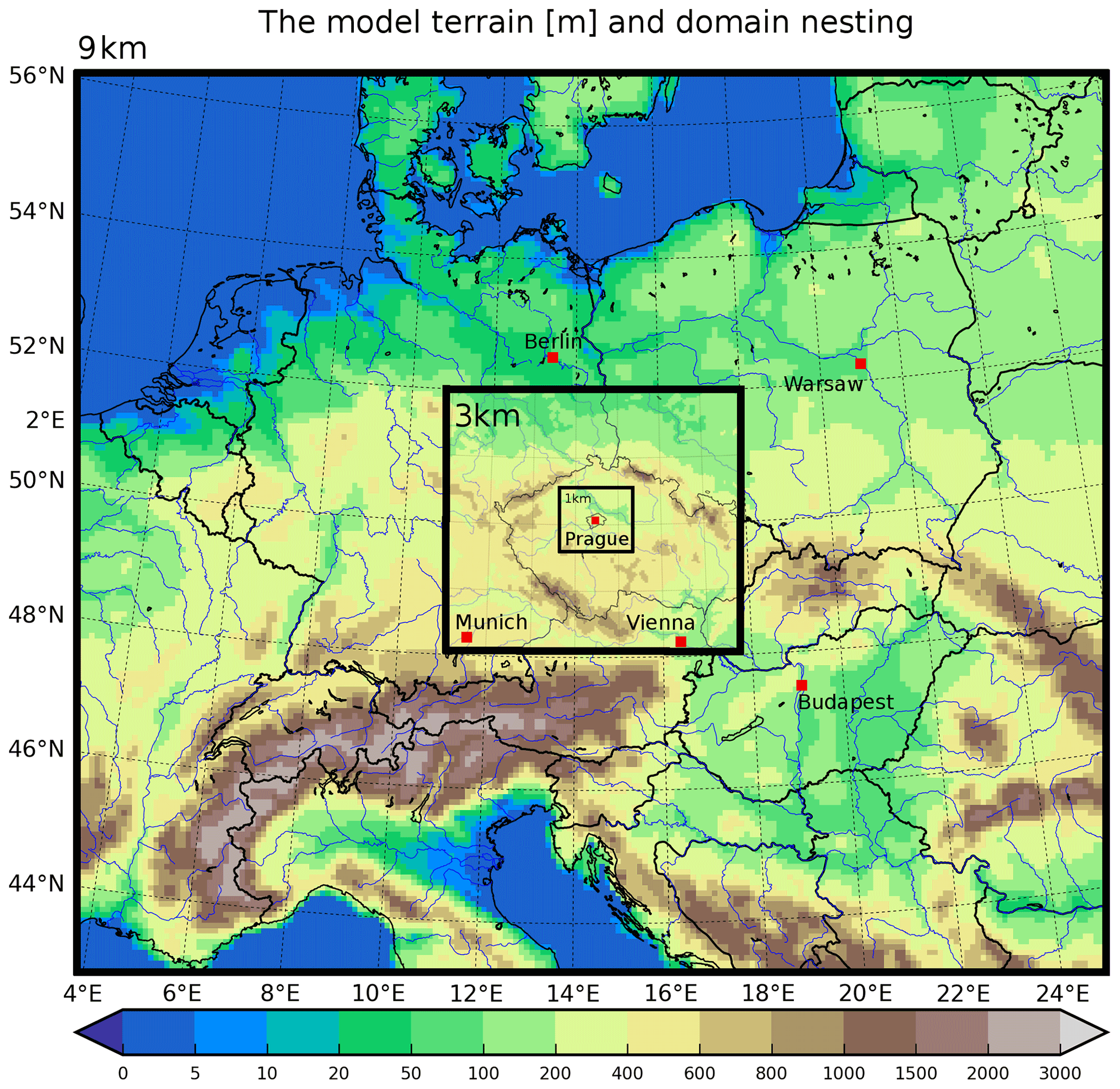
Figure 1The resolved model terrain in meters, the nesting structure and the cities analyzed in the study (Prague, Berlin, Munich, Vienna, Budapest and Warsaw).
For the coarse 9 km domain simulations, the ERA-interim reanalysis (Simmons et al., 2010) is used as climate forcer. The 3 and 1 km domains are forced by the corresponding parent domains with one-way nesting. Chemical boundary conditions (for the outer domain) are taken from the CAM-chem global model data (Buchholz et al., 2019; Emmons et al., 2020). Land use information adopted in model simulations was derived from the high-resolution (100 m) CORINE Land Cover (CLC) 2012 data (https://land.copernicus.eu/pan-european/corine-land-cover, last access: 24 September 2021) and the United States Geological Survey (USGS) database for grid cells without CORINE information. An important difference between WRF and RegCM models is that the latter one, fractional land use, is considered, while in WRF, each grid cell is designated the dominant land use.
2.2.1 Model simulations
To fulfill the goal of the study, several simulations have been performed with and without including the effects of both the urban canopy meteorological forcing and the chemical footprint of the urban emissions (i.e., the UEI). Part of the simulations that are analyzed in this work had been already analyzed in Huszar et al. (2020b): these included experiments with all emissions considered but with or without considering the UCMF. As the focus of this paper is to evaluate the impact of urban emissions, we extend these simulations with those without the inclusion of such emissions (for selected cities). The complete list of simulations performed is included in Table 1. The regional climate simulations included two experiments with the RegCM model, with (“URBAN”) and without (“NOURBAN”) considering the urban canopy meteorological effects (simulated by the CLMU urban module), and two experiments with the WRF-Chem model, again with and without considering urban canopies (simulated by the SLUCM module).
Table 1The list of model simulations performed: the first section contains the RCM simulations that cover the whole analyzed period with the information of whether urban land surface was considered (second column). The second section lists the performed regional CTM experiments – here the second column provides information on the driving meteorological data (not needed in the case of WRF-Chem).
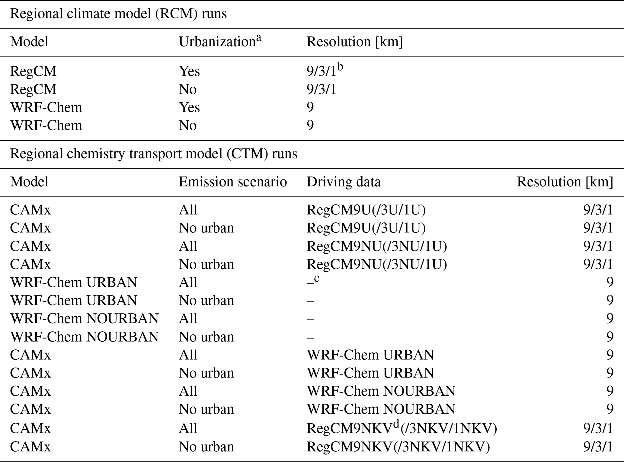
a Information of whether urban land surface was considered. b Simulation performed in a nested way at 9, 3 and 1 km. c No driving meteorological data needed as chemistry is online coupled to the parent meteorological model. d NKV – not considering the urban-induced modifications of the vertical-eddy-diffusion coefficients.
The chemistry transport model simulations encompass CAMx runs based on RegCM and WRF-Chem regional climate reconstructions and that corresponding to the chemical component of WRF-Chem. For each CTM, in total four simulations are repeated. In two, the default emission data (i.e., all emissions) are considered, while the inclusion of urban effect is once included and then excluded. In the other two, urban emissions for selected cities were completely removed (see Sect. 2.2.2), i.e., adopting the annihilation method (Baklanov et al., 2016). Finally, two additional simulations with CAMx driven by RegCM meteorology were performed to analyze the effect of the UCMF-induced changes in the vertical eddy diffusion (Kv) and their contribution to the modeled urban emission impact.
This strategy of experimental design allows us to evaluate the UEI for both the URBAN and NOURBAN cases and analyze their difference or, in other words, to investigate how the emission impact is modulated by the UCMF. Thus, the main focus is on the evaluation of
where the UEI for URBAN or NOURBAN cases is evaluated for a pollutant C as
The relative impact will be evaluated as
for NO2 and PM2.5, i.e., the relative contribution of urban emissions to the total concentration is provided. For O3, UEIi,rel is calculated as
i.e., this number gives the relative change in the concentration after introducing urban emissions.
The relative Δ(UEI) presented throughout the article is calculated as
2.2.2 Emission processing
For Europe, emissions provided by CAMS (Copernicus Atmosphere Monitoring Service) version CAMS-REG-APv1.1 inventory (regional–atmospheric pollutants; Granier et al., 2019) for the year 2015 were used as anthropogenic emissions. For the Czech Republic, the high-resolution national Register of Emissions and Air Pollution Sources (REZZO) dataset issued by the Czech Hydrometeorological Institute (https://www.chmi.cz, last access: 24 September 2021) along with the ATEM traffic emissions dataset provided by ATEM (Ateliér ekologických modelů – Studio of ecological models; https://www.atem.cz, last access: 24 September 2021) was used. These data offer activity-based (SNAP – Selected Nomenclature for sources of Air Pollution) annual emission sums of main pollutants, namely oxides of nitrogen (NOx), volatile organic compounds (VOCs), sulfur dioxide (SO2), carbon monoxide (CO), PM2.5 and PM10 (particles with a diameter less than 2.5 and 10 µm). CAMS' data are defined on a Cartesian grid. On the other hand, the Czech REZZO and ATEM datasets are defined as area, line (for road transportation) or point sources, while in the case of the first these are usually irregular shapes that correspond to counties with resolutions from a few hundred meters to 1–2 km depending on the geometry of the particular shape, so they are appropriate for resolving urban emissions at 1 km domain resolution (in the case of Prague).
Data from the listed emissions inventories are preprocessed using the FUME (Flexible Universal Processor for Modeling Emissions) emission model (http://fume-ep.org/, last access: 24 September 2021; Benešová et al., 2018). FUME is designed primarily for preparation of CTM-ready emission files, including preprocessing the raw input files, the spatial redistribution of the data into the model grid, chemical speciation and time disaggregation of input emissions. Category-specific speciation factors (Passant, 2002) and time disaggregation (van der Gon et al., 2011) are applied to derive hourly speciated emissions for CAMx and WRF-Chem models. Biogenic emissions of hydrocarbons (BVOCs) for CAMx runs are calculated offline using the MEGANv2.1 (Model of Emissions of Gases and Aerosols from Nature version 2.1) emissions model (Guenther et al., 2012) based on RegCM and WRF meteorology. In the case of WRF-Chem experiments, they are calculated online based on the MEGAN approach. The necessary inputs for MEGAN (plant functional types, emission factors and leaf-area-index data) were derived based on Sindelarova et al. (2014).
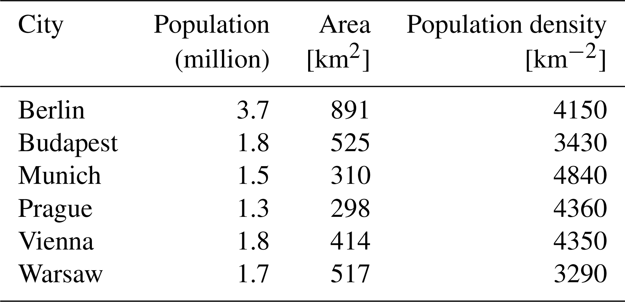
To isolate the emissions originating from urban areas from those from elsewhere, various approaches are possible: one can select the grid boxes (or other shapes) in the source inventories that lie inside the city's limits or the same can be applied for the already redistributed emission on the model grid. Once either approach is selected, first the city boundaries have to be properly defined. For this purpose, we used the Database of Global Administrative Boundaries (GADM) public database (https://gadm.org, last access: 24 September 2021) for the definition of administrative boundaries of the cities selected in this study. For the second task, the masking of inventory emissions based on the GADM shapes corresponding to cities, we had to ensure correct partition between the “city” and “non-city” portion of those shapes which spawn over the city boundaries. For this purpose, the masking capability of FUME was used, which allows us to define an arbitrary mask for subsetting emissions either inside or outside of the mask. To demonstrate the resulting masked emissions for the case of Berlin and Prague at 9 and 1 km resolution, we plotted in Fig. 2 the emissions of NO2 for a selected hour. It is seen that (correctly) only those grid cells that are entirely encompassed within the city have zero emissions. Grid cells that have a part not in the city have non-zero emissions. Cities considered are Prague, Berlin, Munich, Budapest, Vienna and Warsaw, selected based on multiple criteria: (a) city size should be such that at least a few grid cells in the 9 km domain cover the city, (b) cities are sufficiently far from each other to eliminate inter-city influences (see Huszar et al., 2016a), (c) the terrain of the city should have minimal variability to eliminate orographic effects (Ganbat et al., 2015), and (d) cities should be distant from large water bodies and/or sea to eliminate non-symmetric land use effects around the city (e.g., sea breeze effects; Ribeiro et al., 2018). We admit that the selection could follow a more objective criteria like number of inhabitants or area; however, we assumed (and our results showed) that the differences in results between cities are qualitatively very small, and the choice of the list of cities from the region examined has thus a very small effect on the results. Additional information about cities including population, size and population density is included in Table 2. It shows that the cities are of very similar size with populations between 1–2 million inhabitants with Berlin as an exception of a larger city with a population of 3.7 million. Most of the emitted polluting material from these cities is in the form of CO and NO2 (Huszar et al., 2016a). Most of the cities emit primarily in the transport sector, while residential heating and energy production are also important (energy production being the primary source for Warsaw).
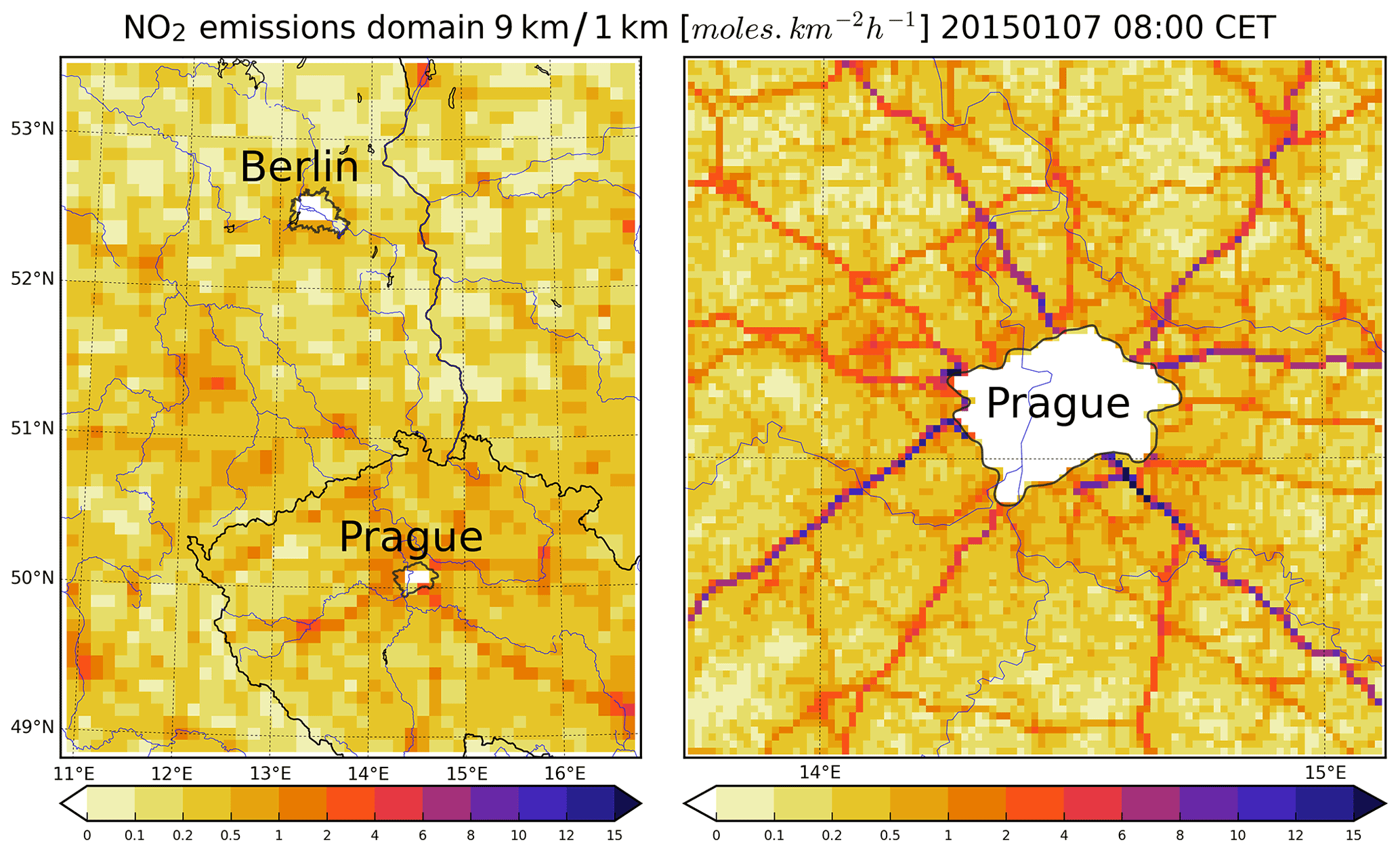
Figure 2Demonstration of the masked NO2 emissions for Prague and Berlin for the 9 and 1 km domains (in ) (only a part of the domains is shown).
3.1 Model validation
Both the regional climate and chemistry transport model experiments presented here (those considering all emissions; see Table 1) were subject to validation in Huszar et al. (2020b) based on European E-OBS (version 20.0e) meteorological and AirBase air quality data (https://www.eea.europa.eu/data-and-maps/data/aqereporting-8, last access: 24 September 2021). Here we summarize only the most relevant conclusions for the validation of meteorological fields, while for the chemical validation, we provide the comparison of the annual cycle of the pollutants in focus for each analyzed city. Regarding meteorology, it was shown that each model performs reasonably within accepted range of biases and is comparable to other studies using very similar model configurations (Berg et al., 2013; Karlický et al., 2017, 2018). In general, RegCM precipitation is well captured in all seasons, while the winter temperatures are somehow larger than measured ones connected probably to reduced thermal cooling. For WRF, precipitation is overestimated mainly during summer and is probably connected to overestimation riming caused by increased graupel sedimentation in deep convective clouds. Furthermore, both models show some overestimation of 10 m wind speeds and a reasonable reproduction of the maximum daily PBL heights with WRF performing better than the RegCM model which slightly overestimates it, caused probably by the strong vertical turbulent transport in the Holtslag scheme that RegCM uses.
The simulated annual variation in monthly mean modeled and measured air quality data is shown in Fig. 3, while for each city, the average of all available urban background stations is used. NO2 is systematically underestimated in all models and all cities by about 10–20 µg m−3, suggesting either low emission values or incorrect speciation in the FUME emission model, supported also by the fact that the diurnal cycles usually are well captured with respect to their shape (only the systematic underestimation mentioned earlier persists). In the case of ozone (O3), it is strongly overestimated (by up to 20–30 µg m−3 in all simulations, being the largest in the RegCM-driven one). In Huszar et al. (2020b) it was shown that this is given mainly by a nighttime positive bias reaching 40 µg m−3 which emerges from inaccuracies in nighttime chemistry and deficiencies in capturing nocturnal vertical eddy transport (Zanis et al., 2011). Huszar et al. (2020b) also showed that high-resolution experiments are more successful in capturing the day-to-day variation in NO2 values probably as a result of the higher resolution of emission data and also due to better representation of the terrain and hence the meteorological conditions. Finally, PM2.5 is usually underestimated in models by around 10 µg m−3 throughout the year with the smallest biases encountered in the WRF-driven CAMx experiment. This negative bias was attributed in Huszar et al. (2020b) to underestimated nitrate aerosol formation and also to strongly underestimated organic aerosol which is an important component of the urban PM2.5 burden. As for the influence of these model deficiencies on the results, the underestimation of NO2 and PM2.5 means that the UEI will be somewhat underestimated too in our models. In the case of ozone, which is usually overestimated except summer maximum values, it is expected that the average impact of UEI (decreases, see below) will be slightly underestimated in the model.

Figure 3Comparison of the modeled average annual variation in monthly means with observations for the six selected cities and three pollutants: NO2, O3 and PM2.5 (in µg m−3). The black line means observations, and red, yellow and sky blue stand for RegCM/CAMx, WRF-Chem and WRF/CAMx models.
3.2 The impact of urban emissions
In our analysis we will focus on the near-surface concentrations of NO2, PM2.5 and O3. First, the impact on seasonal – DJF (winter) and JJA (summer) – averages will be presented. As different emissions and chemical regimes occur during the day, the diurnal cycles are of interest too. Further, given their high policy relevance, the impact on the extreme values will be evaluated as well. Finally, we will look how the vertical turbulent diffusion, as the most important component of UCMF, alone explains the modeled impact of (not) considering the urban canopy meteorological effects.
3.2.1 Seasonal impact
In Fig. 4 the winter UEI for NO2 is presented for the three applied modeling systems: RegCM/CAMx (9 and 1 km horizontal resolution), WRF/CAMx and WRF-Chem (both with only 9 km resolution). The first two columns shows the UEI evaluated from the URBAN experiments, the absolute impact shown in the first one, while the relative contribution of urban emissions to the total concentrations is in the second one. Higher values of the impact of up to 4–6 ppbv are seen for each analyzed city, and the similarities between models are very large. This corresponds to the contribution of urban emissions of around 40 %–60 % for urban centers. The impact quickly becomes small further from cities with increases up to 1 ppbv over rural areas corresponding to about a 5 %–10 % contribution. The impact is not completely symmetric around cities owing to the prevailing wind directions. If calculating the UEI on the 1 km domain (case of Prague), it reveals some details of the emission structure of the city with a maximum impact of 6 ppbv that corresponds to a 60 %–80 % contribution and so providing a somehow larger relative impact for the city core if a higher resolution is applied. The UEI impact evaluated from the NOURBAN is evidently larger (third and fourth columns), exceeding 6 ppbv for each analyzed city and model too. In other words, the impact of city emissions is smaller if URBAN effects are considered, and this difference can reach 2–3 ppbv, especially in the WRF-Chem experiments. The impact over areas surrounding cities is larger in the urbanized runs by about 0.1–0.2 ppbv, quickly becoming zero further from cities where the UCMF becomes negligible. In relative numbers, the decrease in UEI modeled for the URBAN case is about 20 %–40 % and is seen for larger areas not limited to the analyzed cities. However, over areas where both the absolute city impact (UEI) and the difference ΔUEI is small, this relative decrease is a result of the ratio of two very small numbers and should be regarded with caution. This holds for areas where the relative change in ΔUEI is positive, which means stronger urban emission impact for the URBAN compared to NOURBAN case. This is, however, explainable by the fact that in the former case, the stronger urban turbulence removes pollutants more effectively and the deposition occurs at larger distances leading to concentration increase (see Huszar et al., 2020b); although these changes are very small in absolute numbers, so the relative difference between the URBAN- and NOURBAN-based UEI should be again treated with caution.
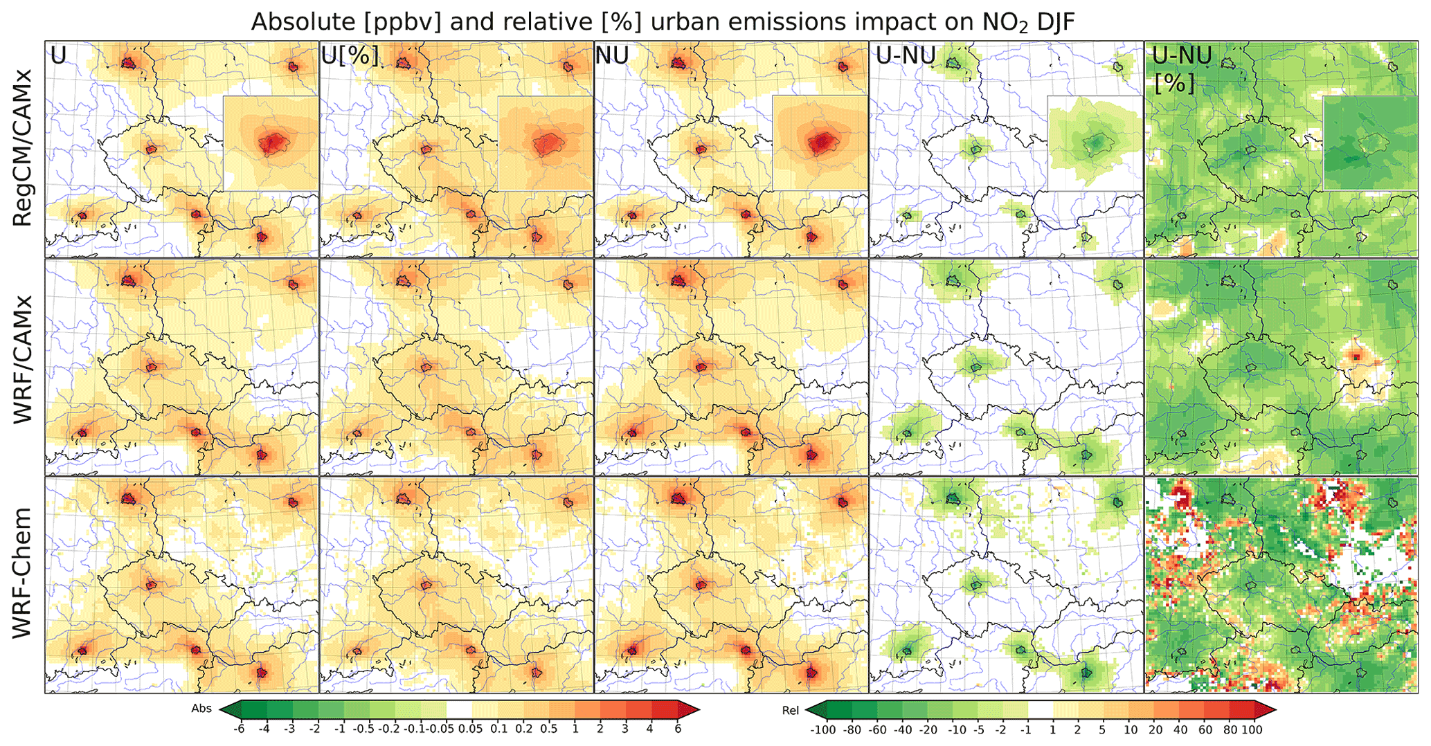
Figure 4The urban emission impact (UEI) of six selected cities (Berlin, Budapest, Munich, Prague, Vienna and Warsaw) on average DJF near-surface NO2 concentrations from 2015 to 2016 for the three modeling systems used: CAMx driven by RegCM (first row), CAMx driven by WRF-Chem meteorology (second row) and WRF-Chem (third row). Individual columns represent the UEI evaluated for the URBAN experiments as absolute (UEIURBAN; U; in ppbv) and relative impact (UEIURBAN,rel; U[%]), the UEI impact for the non-urbanized (NOURBAN) experiments (UEINOURBAN; NU), the difference between the two (ΔUEI; U-NU), and the relative change in the impact (Δ(UEI)rel; in %). The corresponding results for Prague at 1 km resolution from the RegCM-driven CAMx experiments are plotted within the 9 km figures in the upper row.
For the case of JJA in Fig. 5, the results are qualitatively very similar to DJF. The absolute impact of urban emissions is somewhat smaller, usually reaching 4 ppbv and being largest in the RegCM/CAMx model. The spatial extent of the impact larger than 0.05 ppbv is also smaller than in DJF. This is an expected consequence of in general lower summer emissions due to the missing domestic heating source and also due to larger mixing into higher model levels allowing transport to distant areas. The relative contribution of urban emissions to the final concentrations is also smaller than in JJA. The UEI for the NOURBAN case leads again to a higher emission impact reaching 6 ppbv (slightly higher than in the winter case). The spatial extent is, however, smaller than during DJF. This resulted in a different ΔUEI pattern in JJA: the spatial extent of the decrease for the URBAN case is smaller; however, for urban cores, the decrease in the impact is larger compared to DJF. The relative change in the UEI is also larger during this season, often exceeding 60 %.
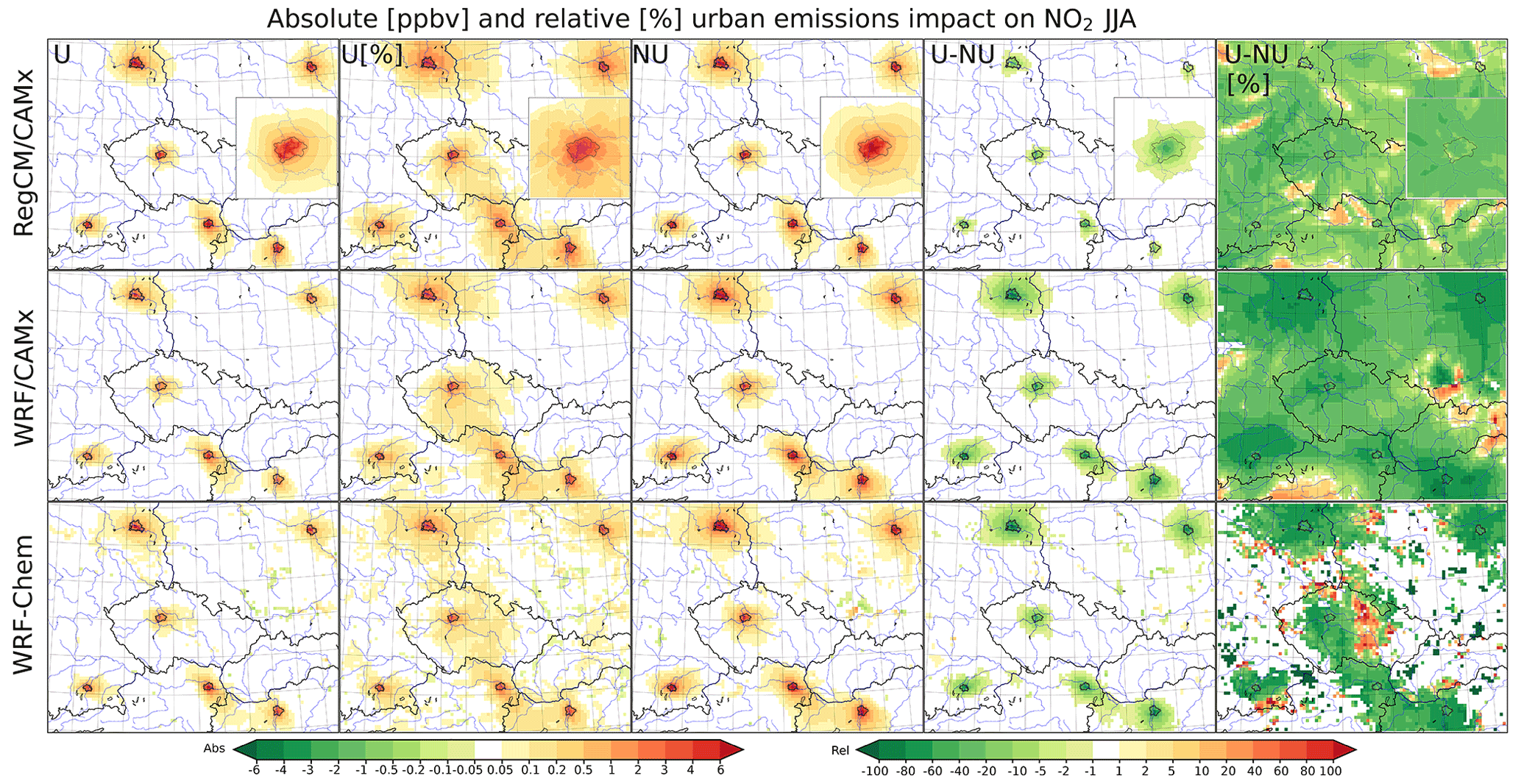
Figure 5Same as Fig. 4 but for JJA.
For PM2.5, again, the general conclusions are similar to NO2. The winter UEI (Fig. 6) reaches 4–6 µg m−3 for the analyzed cities and reaches 0.5 µg m−3 for rural areas. The relative contribution of urban emissions to the PM2.5 concentrations for the city centers and rural areas is about 20 %–40 % and 1 %–5 %, respectively. The UEI evaluated for the NOURBAN case is again stronger, often exceeding 6 µg m−3; the rural impact is, however, very similar to the URBAN case. The decrease in UEI due to the inclusion of urban effects (i.e., the UCMF) is usually between −2 and −3 µg m−3 corresponding to about a 40 %–60 % smaller impact in the URBAN case compared to NOURBAN one for the city centers. The difference between the URBAN and NOURBAN UEI can be even positive, e.g., above rural Poland or also seen around Prague in the 1 km resolution runs. This can be explained by the fact that UCMF causes stronger turbulent removal of the urban emissions, but this results in enhanced sedimentation further from cities leading to higher emission footprint there (especially in the WRF-Chem experiments).

Figure 6Same as Fig. 4 but for PM2.5 (in µg m−3).
During JJA (Fig. 7), the PM2.5 urban-emission-induced concentration changes for both the URBAN and NOURBAN cases resemble the situation in DJF quantitatively, but they are smaller, up to 2 µg m−3 in all models and cities. They are larger, reaching 4 µg m−3 in the high-resolution experiments for Prague where the concentrated character of sources is better resolved. In relative numbers, the contribution makes about 20 %–40 % (except the city core in Prague at high resolution reaching 60 %). If the UCMF is considered, the UEI decreased by about 1–2 µg m−3 with the exception of Prague in high resolution reaching a −3 µg m−3 decrease.

Figure 7Same as Fig. 6 but for JJA.
The impact of urban emissions on regional ozone (Fig. 8) follows a different pattern than for NO2 and PM2.5. As a secondary gas, its responses to increased emissions of its precursors (NOx and NMVOC) depend not only on the magnitude of each precursor but also on their ratio. In the case of CAMx (either driven by RegCM or WRF meteorology), introducing urban emissions resulted in a clear O3 decrease above the selected urban areas reaching a −2 to −3 ppbv decrease as JJA average for the 9 km experiments while exceeding −4 ppbv for Prague at 1 km. In relative numbers, this represents a decrease by up to 10 %–20 % (but usually between −5 % and −10 %) compared to the background concentrations (that do not consider urban emissions). The UEI over rural areas surrounding cities manifests itself as a slight increase in ozone by up to 0.5–1 ppbv (a few percentage points in relative numbers). For the NOURBAN case, the decrease in O3 is stronger for each city, usually exceeding −4 ppbv or even −6 ppbv in the high-resolution runs for Prague. This means that the UEI for ozone is weaker in the URBAN case by around 2–3 ppbv. For areas surrounding cities, where ozone increased due to the urban emissions, the UEI difference between the URBAN and NOURBAN cases is positive too, meaning that the ozone increase due to UEI is larger in the URBAN case. In relative numbers, the change in UEI due to the introduction of the UCMF is often larger than −60 % (stronger in the WRF-driven CAMx runs). For city vicinities, the relative change in UEI reaches high values too, up to 100 % increase.
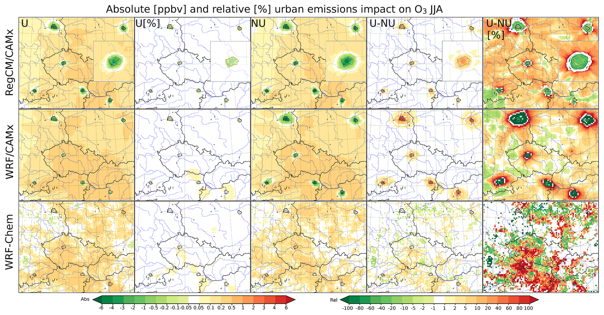
Figure 8Same as Fig. 5 but for O3.
A different picture is gained if the UEI is evaluated for ozone based on the WRF-Chem model. The addition of urban emissions leads here to either no change or a little increase in the average summer ozone, indicating a different ozone isopleth pattern in the case of the RADM2 mechanism used in the mentioned model (for more details, see the Discussion). For most of the analyzed cities, the UEI means about a 0.5 ppbv increase in ozone, while for Berlin, it is rather characterized by a slight decrease (around −0.1 ppbv). These slight changes constitute a very small relative change on the order of up to 5 %. The UEI is slightly smaller in magnitude in the NOURBAN case. In relative numbers one obtains a rather complicated pattern; however, it is a result of the ratio of very small, almost insignificant changes. What one can state for certainty is that in the WRF-Chem model, urban emissions lead to a rather slight ozone increase above cities which is stronger in the URBAN case than in the NOURBAN one.
3.2.2 Impact on diurnal cycles
As the UCMF has a different magnitude throughout the day (e.g., the urban warming or heat island has a clear peak during early night hours, while the urban boundary layer is thickest during the day), one might expect that the different impacts of urban emissions between the URBAN and NOURBAN cases will have a specific diurnal cycle too. We therefore calculated the average seasonal diurnal cycles of concentrations from the analyzed urban centers (averaged over all city).
Figure 9 shows the DJF and JJA average diurnal cycles for surface NO2 concentrations from individual simulations and their differences (i.e., the UEIs and the ΔUEIs). In general, the three models perform in a very similar manner. The UEI impacts for both the NOURBAN (blue) and URBAN (orange) cases follow strongly the typical pattern for the NOx emissions exhibiting two peaks during morning and afternoon rush hours (the weekends have a somewhat weaker pattern, but weekdays dominate the average). It is clear that the UEI for URBAN case (dashed orange) is much lower, reaching 10–15 and 5–10 ppbv as peaks in DJF and JJA, respectively, while the difference with respect to the NOURBAN-based UEI (dashed blue) varies during the day. Its exact diurnal pattern is shown by the green line which has a very clear pattern in both seasons and all models (belongs to right vertical axis). In absolute sense it is almost zero during nighttime and reaches its maximum during early evening hours. In RegCM-driven CAMx the maximum reaches −3 to −4 ppbv for DJF and JJA, respectively, while a much stronger decrease is modeled with WRF meteorology reaching −12 ppbv. This is a much greater change in UEI (due to the UCMF) than seen for the seasonal means in Figs. 4 and 5. A second, smaller peak during morning hours is also exhibited by each model that reaches values between −1 to −4 ppbv.
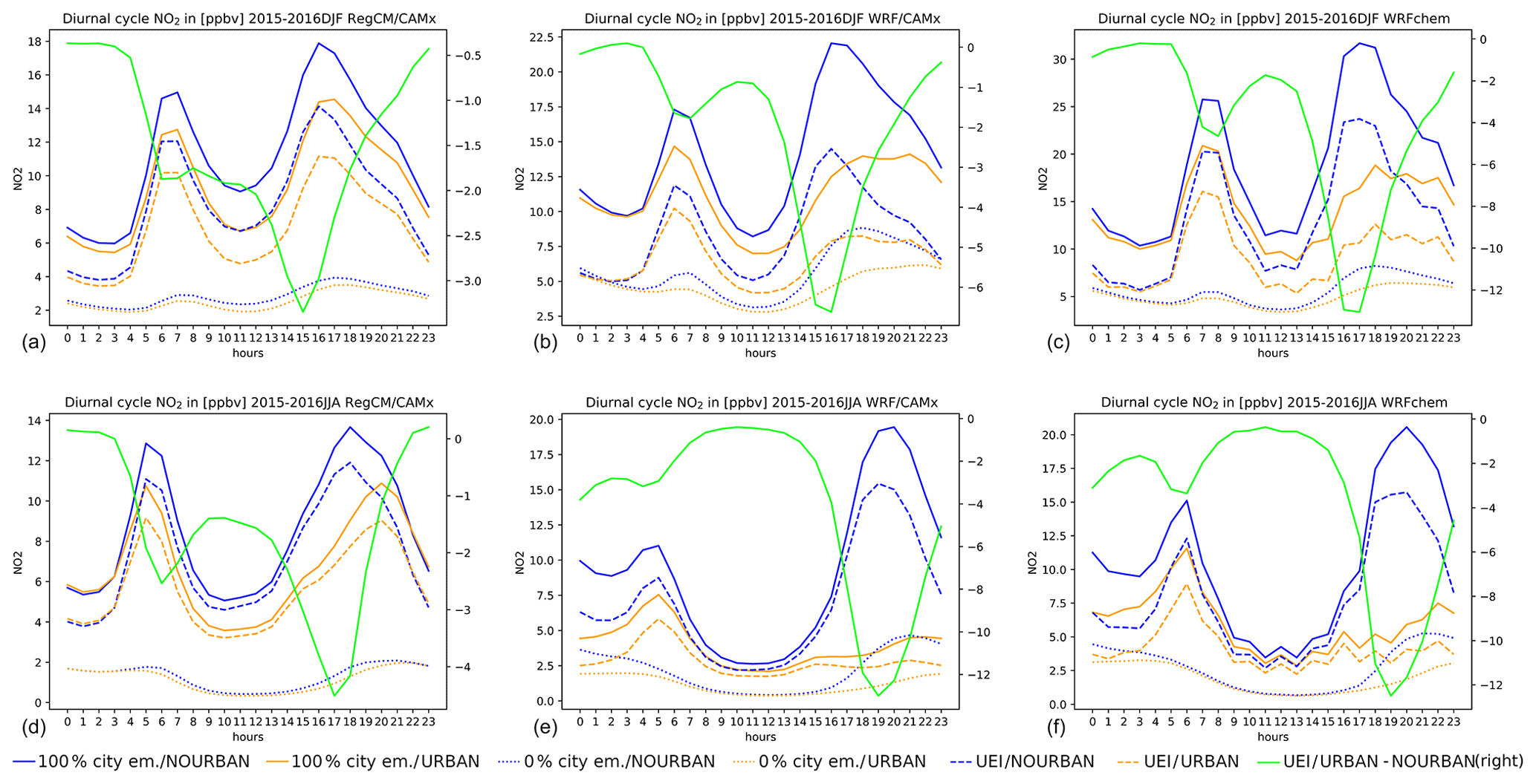
Figure 9The average diurnal cycle of the absolute urban NO2 concentrations and their difference between different simulations for DJF (a–c) and JJA (d–f) and for the three models applied as columns: CAMx driven by RegCM, CAMx driven by WRF and WRF-Chem. Blue and orange lines denote the NOURBAN and URBAN cases, respectively. Solid lines stand for the reference values with 100 % urban emissions, dotted lines for the 0 % urban emission runs and dashed ones for the UEI evaluated for both the NOURBAN and URBAN cases. These correspond to the left vertical axis. Finally, the green line denotes the ΔUEI (right vertical axis), i.e., the modification of the urban emission impact due to the inclusion of the urban effects (the UCMF). Units in parts per billion volume (ppbv).
A qualitatively very similar result is obtained for PM2.5 (Fig. 10). Again, the three models provide comparable results. The UEI impacts for both the NOURBAN and URBAN cases follow strongly the typical pattern for the PM2.5 emissions exhibiting two peaks during rush hours. It is clear that the UEIs for the URBAN case are much lower reaching 4–6 and 2–3 ppbv as peaks in DJF and JJA, respectively, while the difference with respect to the NOURBAN UEI case varies during the day. Its exact diurnal pattern is shown by the green line which, again, has a very clear pattern in both seasons and all models. In absolute sense it is almost zero during nighttime and reaches its maximum during early evening hours. In RegCM-driven CAMx the peak reaches −1.4 and −1.2 µg m−3 for DJF and JJA, respectively, while a much stronger decrease is modeled with WRF meteorology reaching −5 µg m−3 in DJF (−3.5 µg m−3 during JJA). Similarly to NO2, this is a much greater change in UEI (due to the UCMF) than seen for the seasonal means in Figs. 6 and 7. A second, usually much smaller peak during morning hours is also exhibited by each model that reaches values between −1 to −2 µg m−3.
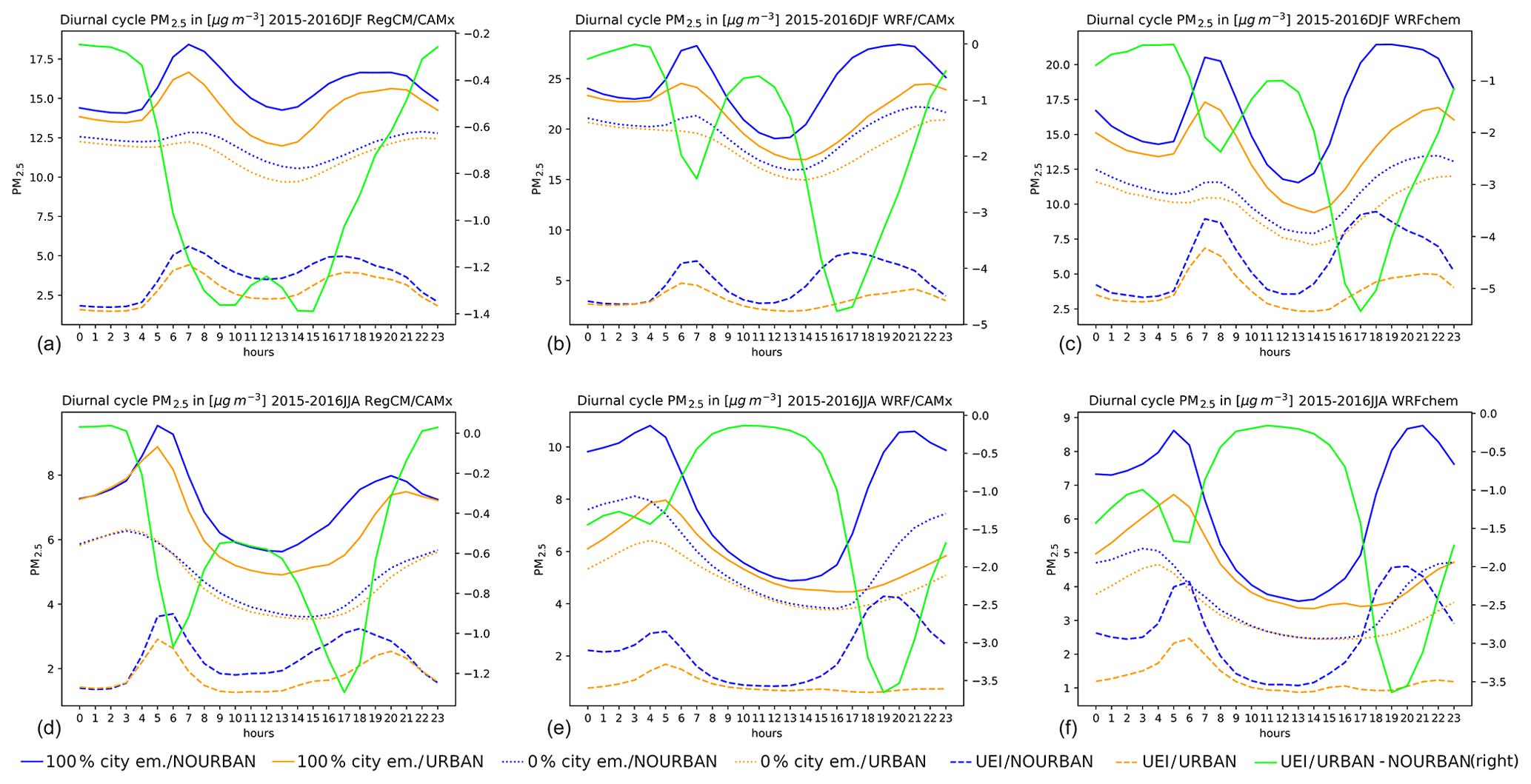
In the case of ozone (Fig. 11), for the CAMx experiments, the UEI shows a strong correlation with the absolute values (dashed vs. solid lines) meaning that when urban ozone values are lowest, also the UEI for O3 shows its maximum (in absolute sense). The maximum impact occurs during morning and early evening hours, reaching −12 and −10 ppbv for DJF for the NOURBAN and URBAN cases, respectively, and reaching minimum values during noon and night. During JJA, the UEI reaches −10 and −8 ppbv for the NOURBAN and URBAN cases, while the UEI for the URBAN case is smaller in the WRF-driven CAMx experiment (reaching −5 ppbv). In conclusion, in CAMx driven either by RegCM or WRF, the UEI is negative during the whole day. in the case of WRF-Chem, the impact is expectedly negative throughout the whole day in DJF, but for summer, it becomes positive during daytime, reaching 1.5 ppbv (the URBAN case being slightly higher). During night, the UEI reaches negative values of up to −1 ppbv for the NOURBAN case and −0.2 ppbv for the URBAN one. The ΔUEI (green line) is rather positive in each model and season showing a clear maximum during late afternoon and evening hours, which reaches a few parts per billion volume in DJF (0.5 in WRF-Chem), while in JJA the maximum can be as high as 10 ppbv. This indicates that the urban emission impact for ozone is smaller in absolute sense if the model predicts its decrease due to UEI (CAMx), while it is higher if the model predicts an increase (WRF-Chem).
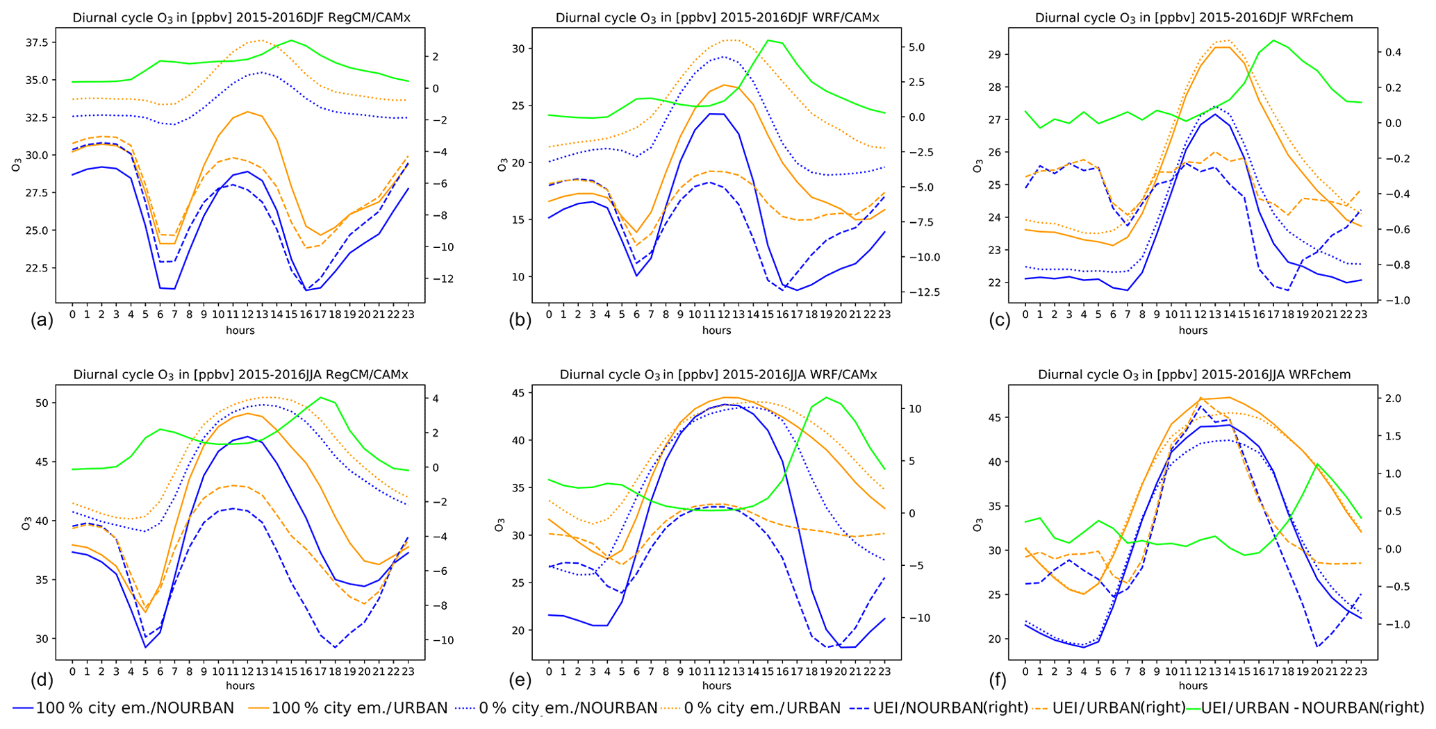
Figure 11The average diurnal cycle of the absolute urban O3 concentrations and their difference between different simulations for DJF (a–c) and JJA (d–f) and for the three models applied as columns: CAMx driven by RegCM, CAMx driven by WRF and WRF-Chem. Blue and orange lines denote the NOURBAN and URBAN cases, respectively. Solid lines stand for the reference values with 100 % urban emissions, while dotted lines are for the 0 % urban emission runs (both belonging to the left vertical axis). Dashed lines mean the UEI evaluated for both the NOURBAN and URBAN cases, and the green line denotes the ΔUEI (right vertical axis). Units in parts per billion volume (ppbv).
3.2.3 Impact on extreme values
Huszar et al. (2020b) showed that the urban canopy meteorological forcing has a stronger effect on extreme air pollution (95th percentile of NO2, PM2.5 and O3) compared to the average one. This motivates us to look also at the UEI for such situations. We therefore plotted the UEI on the 95th percentile values of the daily means of the analyzed pollutants and were interested also in the associated differences between the UEI evaluated for the NOURBAN and URBAN cases (i.e., ΔUEI). In Fig. 12 we see that the UEI for the 95th percentiles of NO2 is much higher compared to the impact on the average one and reaches 9–12 ppbv, especially in the WRF-Chem model (left column). It can also be seen that it reaches 4–6 ppbv (i.e., the values seen for the averages) at distances roughly twice the city size, indicating the crucial role urban emissions play in extreme air pollution events at regional scales. Regarding the modulation of the emission impact by the UCMF (the right column), it is seen that it is also much higher compared to the difference in the case of averages and can reach −6 ppbv. This means that the UEI on extreme air pollution is even more strongly reduced by the urban effects that the averages seen in Figs. 4–5.
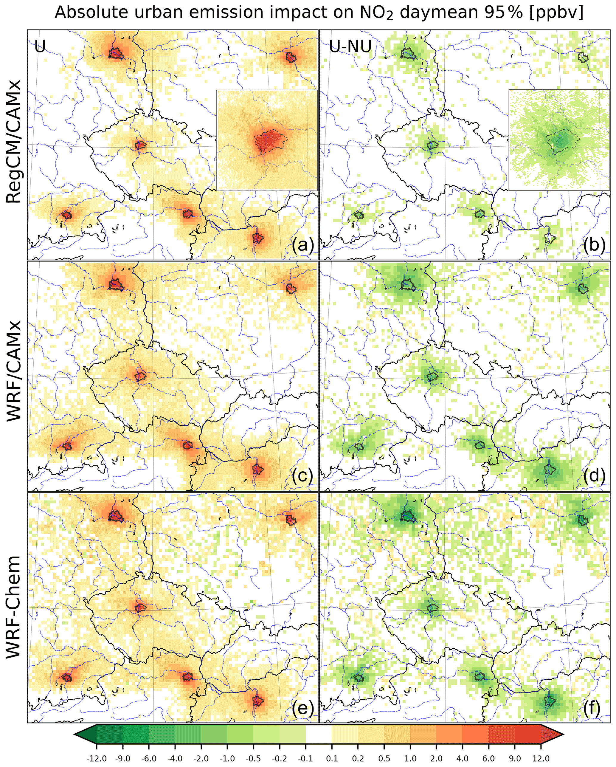
Figure 12The impact of urban emissions (UEI) for selected cities (Berlin, Budapest, Munich, Prague, Vienna and Warsaw) on the 95th percentile of the daily mean NO2 concentrations for the three models (as rows) for the 2015–2016 period: the left column shows the absolute UEI for the URBAN case, while the right column denotes the ΔUEI, i.e., the difference between the UEI for the URBAN and NOURBAN cases. Results from the 1 km×1 km experiment are plotted within (a) and (b). Units in parts per billion volume (ppbv).
In the case of PM2.5 in Fig. 13, the UEI for the 95th percentiles is again higher than calculated for the averages and reaches 8 µg m−3 in each model (especially for Prague, Budapest and Warsaw). This is again higher than the impact on averages (up to 6 µg m−3) and points to the increased role of urban emissions during extreme PM pollution events. Our results also suggest a large impact over rural areas reaching 1–2 µg m−3, indicating potential for urban emissions to enhance rural concentrations too. The decrease in the UEI of extreme values of PM2.5 if the UCMF is considered can be as large as −4 to −6 µg m−3. Again, this is a stronger decrease compared to the values obtained for the DJF and JJA averages (Figs. 6–7).
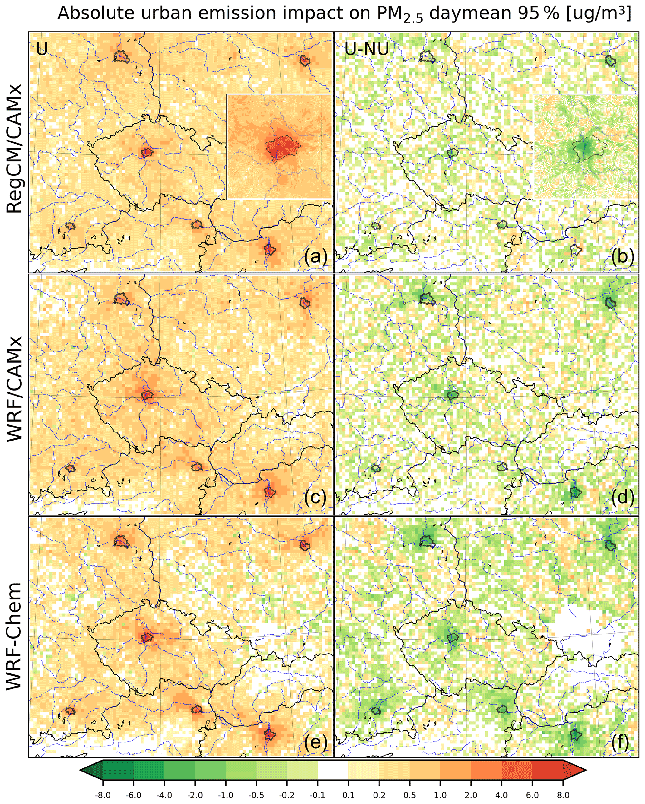
Figure 13Same as Fig. 12 but for PM2.5 (in µg m−3).
In the case of ozone (Fig. 14), somehow different behavior is modeled for CAMx and for WRF-Chem (similarly to the impact on seasonal averages), but differences are encountered between cities too. The UEI for the 95th percentile of the daily maximum 8 h O3 is usually negative over cities, reaching −4 ppbv over city cores – this is the case of RegCM/CAMx and partly in WRF/CAMx too (for Berlin, Warsaw, Prague and Budapest) with smaller decrease up to −1 ppbv. These are smaller decreases that those seen for average JJA ozone in Fig. 8. On the other hand, for cities like Budapest and Berlin in WRF/CAMx experiments and for all cities in WRF-Chem, the UEI for the 95th percentile ozone values is positive with increases up to 2–4 ppbv in WRF-Chem. For areas surrounding cities, further from the origin of the emissions, there is a clear increase in ozone reaching 1 ppbv over large areas. This indicates that during extreme ozone periods, urban emissions push the balance between the ozone production and reduction towards production leading to smaller reductions for some cities and models and stronger increase for other cities and models. The change between the URBAN and NOURBAN cases is positive for RegCM/CAMx similarly to the impact on averages, meaning that the reduction of extreme ozone is smaller when the UCMF is considered, but this modification is smaller than that seen for average values. For other models, the modulation of UEI between URBAN and NOURBAN is rather small and can be negative or positive with the preference of negative change, i.e., enhancement of the UEI in the case of the WRF-Chem model. This means that if extreme ozone responds to urban emissions with an increase, the increase is smaller if UCMF is considered. On the other hand, if ozone responds with a decrease, then this decrease is smaller in absolute values when not considering UCMF.
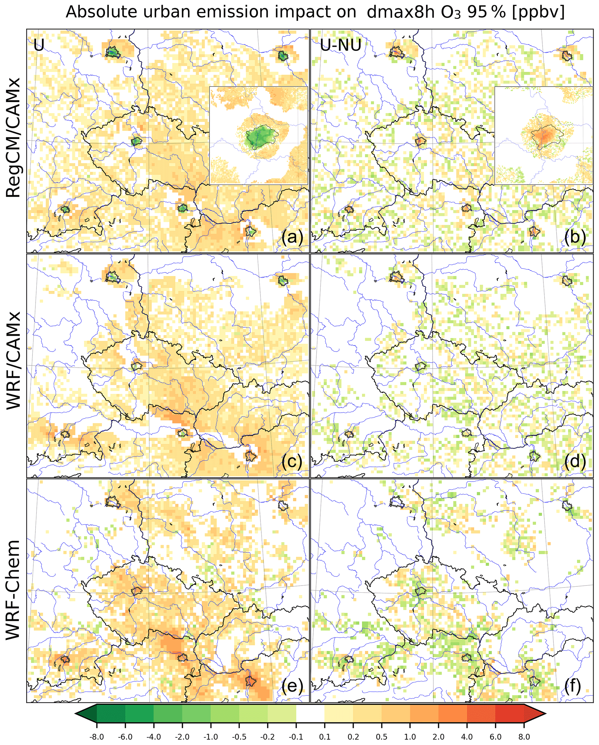
Figure 14Same as Fig. 12 but for the maximum daily 8 h O3 in parts per billion volume (ppbv).
3.2.4 The role of vertical turbulence
As seen in previous sections, the urban emission impact is significantly perturbed if the urban canopy meteorological forcing is considered in its model estimation, and it is usually overestimated if UCMF is disregarded. Many previous studies showed that the most important component of the UCMF influencing the urban air pollution is the vertical eddy diffusion (e.g., Zhu et al., 2015; Huszar et al., 2020a). To evaluate its role and contribution to the changes in UEI between the URBAN and NOURBAN cases, we performed additional simulations with the effect of perturbed vertical-eddy-diffusion coefficients (Kv) removed (denoted as “NKV”). To estimate the effect of Kv changes alone, we computed the UEI for the NKV case too and compared it to UEI obtained for the URBAN case.
In Fig. 15, the diurnal variations in the UEIs calculated for the NOURBAN and URBAN cases, as well as for the NKV case, are presented. Besides, it shows the modulation of the UEI due to the consideration of all components of the UCMF, as well as due to the consideration of only the Kv effects. In the case of NO2, it is evident that the diurnal cycle of the UEI calculated for the NOURBAN case is very close the cycle for the NKV case, and this holds for both DJF and JJA. In other words, the modulation of this impact by considering all urban effects (URBAN case) is almost the same if taking for reference the NOURBAN or NKV case. This means that the vertical-eddy-diffusion component of the UCMF alone explains the modeled modulation of UEI due to the UCMF. The differences arise from the fact that the UCMF also contains the component of decreased wind and increased temperature (Huszar et al., 2018b, 2020a), and especially the wind's effect causes the urban concentrations to be higher due to lower wind speeds and limited dispersion. This implies a higher UEI in the NKV case compared to NOURBAN case because wind stilling is present. Adding the Kv effects leads to slightly lower UEI, but it is clear that the turbulent eddy diffusion dominates the UEI.
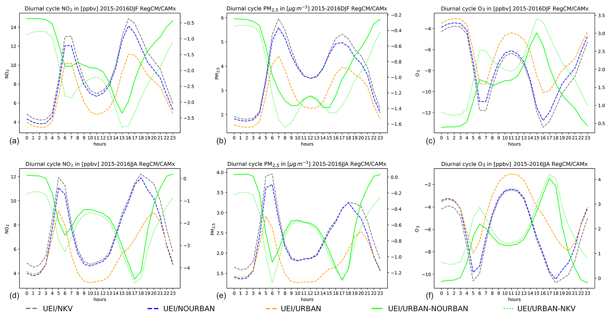
Figure 15Impact of considering the vertical eddy diffusion (Kv) on the urban emission impact (ΔUEI) calculated from RegCM/CAMx simulations for DJF (a–c) and JJA (d–f) for NO2 (a, d), PM2.5 (b, e) and O3 (c, f). Dashed grey, blue and green lines stand for the UEI calculated from the NKV, NOURBAN and URBAN cases, respectively, and belong to the left y axis. Solid and dotted green lines denote the ΔUEI as the difference between the URBAN and NOURBAN and between the URBAN and NKV cases. Gases is in parts per billion volume (ppbv) and PM2.5 in micrograms per cubic meter (µg m−3).
The situation is similar for PM2.5, showing that the diurnal cycle of UEI for the NOURBAN case is very close to the cycle calculated for the NKV case with the highest differences during the morning and afternoon peak hours. Consequently, the modulation of UEI due to all components of UCMF vs. due to Kv effects only is very similar, especially during JJA. Finally, the situation for O3 follows the conclusions for the previous two pollutants. The UEI based on the NOURBAN and NKV shows very similar decreases with differences less than 0.5 ppbv. This implies that the ΔUEI due to all urban effects is again very close to that due to Kv effects only, especially during JJA.
In summary, the modulation of the urban emission impact due to the UCMF is largely determined by the action of the enhanced vertical eddy diffusion. The effect of other components is small and explains the slight difference between the UEI calculated for the NOURBAN vs. NKV cases.
This study looked at the regional air quality impact of urban emissions (UEI) from selected large cities and agglomerations in central Europe with the focus of quantifying not only the UEI magnitude but also the modulation of UEI due to the consideration of the urban canopy meteorological forcing (UCMF). The UCMF was calculated from a pair of runs (with and without considering urban land cover) for two regional climate models, RegCM and WRF-Chem, while the UEI was quantified using CAMx driven by both of these models and also by WRF-Chem itself, using the annihilation method meaning that urban emissions were completely removed in the reference run and compared to the full emission run.
Before discussing the obtained results, the model's performance with respect to the measurements has to be evaluated. This study did not explicitly perform a model evaluation because the “full” emission model runs were already validated in Huszar et al. (2020b). Based on a comparison to urban ground sites, they found a systematic underestimation of both NO2 and PM2.5 throughout the year and also in the daily cycles. This indicates an underestimation of urban emissions, and consequently it also means the UEI simulated in this study might be somehow underestimated. Similar underestimation of PM2.5 was also encountered in Ďoubalová et al. (2020) who applied CAMx coupled offline to WRF using almost identical emissions over roughly the same domain, as well as previously by Huszar et al. (2018a, b) and Huszar et al. (2020a) too. The modeled negative PM2.5 bias can be attributed to the underestimation of aerosol components like nitrates and organic aerosol, as seen – similarly to our results – in Schaap et al. (2004) and Myhre et al. (2006). However, besides underestimated emission inventory values, daytime dilution that is too strong and overestimated vertical turbulence can probably play a role too, as argued by Nopmongcol et al. (2012). Indeed, there is a large uncertainty in calculating the vertical eddy diffusion for urban pollutants (Huszar et al., 2020a) which can strongly reduce near-surface concentrations if too strong. Regarding NO2, the underestimation is very similar to Karlický et al. (2017) and Tucella et al. (2012) who used WRF-Chem over Europe too, although with slightly different emission inventory data.
The validation in Huszar et al. (2020b) also showed a strong overestimation of ozone in monthly means caused mainly by the overestimation of nighttime ozone, while daytime values are captured reasonably. This behavior was attributed to deficiencies in nighttime chemistry and also inaccurately resolved vertical mixing in the nocturnal boundary layer (Zanis et al., 2011). On the other hand, the maximum 8 h ozone values were underestimated in Huszar et al. (2020b), which points to the fact that models are unable to resolve the highest ozone values correctly. This is also one of the main conclusions in the comprehensive Air Quality Model Evaluation International Initiative (AQMEII) model intercomparison presented by Im et al. (2015). As nighttime ozone is overestimated in our simulations, we can expect that the titration effects are underestimated. Consequently, the simulated O3 decreases due to UEI are also probably underestimated.
Our results showed that the urban contribution of NO2 can reach 40 %–60 % in urban cores, meaning that roughly half of the urban NO2 originates from elsewhere (rural sources, smaller cities, etc.). This contribution corresponds to the numbers in Huszar et al. (2016a) who calculated an average annual impact of 42 % averaged over a large number of European cities. Im and Kanakidou (2012) modeled even higher contributions, 90 %–95 % for eastern Mediterranean cities, indicating that the role of local emission can be even higher, especially in cities with greater rural–urban contrast or if higher resolution is used. Indeed, our 1 km runs for Prague showed a 60 %–80 % contribution. As the emitted NOx quickly decays to HNO3 as the urban plume is diluted, the contribution becomes very small further from cities, reaching around 5 %–10 %, again very similar to values in Huszar et al. (2016a) and Guttikunda et al. (2005). Although not analyzed in this study, Guttikunda et al. (2003) found similar values of contribution for SO2.
More importantly, we showed that by considering the urban canopy meteorological forcing, the contribution of urban NO2 becomes lower by about 20 %–40 %. This is an important result as it clearly says that the impact of urban emissions is overestimated if the urban canopy is not properly represented in regional modeling. This further means that the background concentrations (i.e., those with zero urban emissions) are not so strongly affected by UCMF as the “full” emissions, generating this modification of the UEI. This is in line with previous studies that looked at the UCMF impact on urban NO2 levels. For example, Huszar et al. (2018a) presented decreases of about 1–2 ppbv similarly to our change in the UEI. Struzewska and Kaminski (2012) also found a comparable reduction in NO2 due to UCMF, as well as Kim et al. (2015) who showed that due to increased turbulence over cities, NO2 levels are strongly reduced.
The general conclusions for PM2.5 are very similar to NO2. The contribution of urban emissions in the analyzed cities is around 20 %–40 %, which is similar to the values in Huszar et al. (2016a) who simulated a 30 %–60 % contribution. Again, a larger contribution, in both relative and absolute numbers, was simulated by Im and Kanakidou (2012) probably due to lower background pollution. The contribution to rural areas is also similar to the mentioned studies (around 1 %–5 %). Our analysis showed, analogously to NO2, that if the urban canopy effects are considered, the impact on PM is smaller by around 50 %. In other words, if the UCMF is not considered, the impact of urban emissions on PM is strongly overestimated. The reasons for this are again in the action of urban canopy by modifying vertical eddy diffusion, wind speeds and temperature. Indeed, Huszar et al. (2018b, 2020a), Kim et al. (2015), Zhu et al. (2017), and Wei et al. (2018) all modeled decreased aerosol concentrations over urban areas as a result of considering the urban canopy effects and further identified that the most important factor that contributes to this decrease is the enhanced vertical turbulence.
In the case of the impact on O3, different behavior is encountered between the models. While CAMx responds to decreases in near-surface concentrations, a distinct behavior is seen for WRF-Chem with almost no change in concentrations or a slight increase in average JJA ozone. As ozone is a secondary pollutant, its response to elevated emissions (like adding urban emissions to rural ones) can have both signs depending on the ratio of the precursor emissions: NOx and NMVOC. Cities are characterized with a high NOx-to-VOC ratio (Beekmann and Vautard, 2010), and the response to emission changes depends on the slope of ozone isopleths at a given initial ratio. CAMx applied the Carbon Bond 5 chemical mechanism, and Nopmongcol et al. (2012) showed that a 100 % increase in emissions leads to ozone decreases in their analysis based on ozone isopleth for London and summer conditions. This is in line with our study also leading to ozone decreases using the same chemical mechanism. Huszar et al. (2016a) for a large number of central European cities and Im et al. (2011a, b) for Mediterranean cities also showed similar decreases in ozone in urban cores. As already said, in the case of WRF-Chem ozone responded in a different way. For the RADM2 mechanism, which is used by WRF-Chem, Stockwell et al. (2011) showed based again on ozone isopleth analysis that for emission changes in NOx and NMVOC at a ratio around 0.2, the ozone change is minimal. Indeed, for our cities, the average emission ratio is between 0.15 and 0.25. This explains the minimal ozone response modeled for WRF-Chem above cities. For both CAMx and WRF-Chem, further from cities, urban emissions lead to ozone increases. This is not surprising as when urban NOx-rich emissions are diluted and mixed with rural emissions with a higher ratio, ozone production occurs (Poupkou et al., 2008).
Regarding the modulation of the urban emission impact on O3 due to UCMF, the decrease seen in CAMx became smaller, almost by 60 %. In other words, the ozone reduction in a city's core is simulated too high if urban canopy effects are not considered in the regional climate model calculations. For WRF-Chem, as the ozone response was weak, the consideration of urban effects leads to only a slight increase in the impact; i.e., if the UCMF is not considered, the ozone response to urban emissions is smaller. In either CAMx or WRF-Chem, the ozone response to the inclusion of UCMF is in line with previous studies dealing with the urban canopy effects on air quality. Wang et al. (2007, 2009), Ryu et al. (2013), Huszar et al. (2018a), and Li et al. (2019) simulated ozone increase due to UCMF too and attributed it mainly to the dominating effects of increased vertical removal of NOx and consequent reduced titration, while the nocturnal downward turbulent flux of residual ozone can be also important (Huszar et al., 2018a).
The diurnal cycles revealed an important fact: the decrease in the UEI due to the UCMF is not uniform during the day but has a clear maximum during late afternoon and evening hours for both NO2 and PM2.5. This is caused by the timing of the maximum effect of UCMF seen in Huszar et al. (2018a, b). As shown in Kim et al. (2015) and more in detail in Huszar et al. (2020a), the modifications of the vertical-eddy-diffusion coefficients, which are the dominant component of the UCMF, are largest during these times of day, counteracting the decrease in wind speed during evening hours (Karlický et al., 2018). This means that the largest vertical mixing of these pollutants occurs during these times, and hence the largest reduction of the emission impact occurs. A secondary maximum of the UEI reduction is encountered during morning hours. During that time the turbulence enhancement is rather small, but the emissions are high due to the morning rush hour and hence the high modification of the impact which is proportional to the quantity of the emitted pollutants. In the case of ozone, the maximum of the UEI change also occurs during late afternoon and evening hours, and it is again most probably related to the maximum of the modifications of vertical turbulence.
Indeed, our sensitivity analysis focusing on the isolated impact of vertical-eddy-diffusion modifications showed very similar diurnal cycles for the UEI modulation to those caused by the total UCMF impact (which includes additional effects of temperature, wind, moisture, etc.; see Karlický et al., 2020). This confirms the conclusion of studies about the role of urban turbulence triggered either mechanically or thermally (via urban heat island, anthropogenic heat, etc.), which strongly modulates the air pollution (Kim et al., 2015; Zhu et al., 2015, 2017; Xie et al., 2016a, b).
Based on this study, we can conclude that the local and regional footprint of urban emissions over central Europe is strong, but large differences arise from whether the urban-canopy-related meteorological effects, like enhanced turbulence, urban heat island, reduced wind speed, etc., are considered. Based on three modeling systems, we showed that the impact on near-surface NO2 and PM2.5 is reduced if they are taken into account. In the case of ozone, the modulation of the emission impact depends on the emission impact itself: if it is negative and ozone decreases due to urban emissions, then this decrease is reduced if UCMF is considered. On the other hand, if ozone increases due to urban emissions, UCMF causes this increase to be even larger. In any case, we argued that the urban canopy and all the resulting effects on meteorological processes have to be properly accounted for in regional models when the transport of pollutants from urban areas is studied and the impact of such emissions is quantified.
The RegCM4.7 model is freely available for public use at https://github.com/ictp-esp/RegCM, (Giuliani, 2021). CAMx version 6.50 is available at https://www.camx.com/download/ (ENVIRON, 2018). The WRFCAMx preprocessor is available from https://www.camx.com/download/ (ENVIRON, 2018). WRF-Chem version 4.1 can be downloaded from https://www.acom.ucar.edu/wrf-chem/download.shtml (WRF, 2020). The RegCM2CAMx meteorological preprocessor used to convert RegCM outputs to CAMx inputs is available upon request from the main author. The complete model configuration and all the simulated data (3D hourly data) used for the analysis are stored at the Dept. of Atmospheric Physics of the Charles University data storage facilities (about 40 TB) and are available upon request from the main author.
PH provided the scientific idea, the design of the model experiments and the project coordination and supervised the writing of the paper. PH and JK were responsible for performing the RegCM, CAMx and WRF-Chem experiments. JM, TN, LB and ML contributed to the evaluation of the results.
The contact author has declared that neither they nor their co-authors have any competing interests.
Publisher's note: Copernicus Publications remains neutral with regard to jurisdictional claims in published maps and institutional affiliations.
This work has been funded by the Czech Science Foundation (GACR) project no. 19-10747Y and partly by projects PROGRES Q47 and SVV 260581/2020 – Programmes of Charles University. We further acknowledge the CAMS-REG-APv1.1 emissions dataset provided by the Copernicus Monitoring Service, the Air Pollution Sources Register (REZZO) dataset provided by the Czech Hydrometeorological Institute and the ATEM Traffic Emissions dataset provided by ATEM (Studio of ecological models). We acknowledge the E-OBS dataset from the EU-FP6 project UERRA (http://www.uerra.eu, last access: 24 September 2021) and the Copernicus Climate Change Service, the data providers in the ECA&D project (https://www.ecad.eu, last access: 24 September 2021), and the data providers of AirBase European Air Quality data (https://www.eea.europa.eu/data-and-maps/data/aqereporting-8, last access: 24 September 2021) and AIM (Automatic Emission Monitoring network data; http://portal.chmi.cz/aktualni-situace/stav-ovzdusi/prehled-stavu-ovzdusi?l=en, last access: 24 September 2021).
This research has been supported by the Grantová Agentura České Republiky (grant no. 19-10747Y), the Univerzita Karlova v Praze (grant no. PROGRES Q47), and the Univerzita Karlova v Praze (grant no. SVV 260581/2020).
This paper was edited by Stefano Galmarini and reviewed by three anonymous referees.
Baklanov, A., Molina, L. T., and Gauss, M.: Megacities, air quality and climate, Atmos. Environ., 126, 235–249, https://doi.org/10.1016/j.atmosenv.2015.11.059, 2016. a, b
Barnes, M. J., Brade, T. K., MacKenzie, A. R., Whyatt, J. D., Carruthers, D. J., Stocker, J., Cai, X., and Hewitt, C. N.: Spatially-varying surface roughness and ground-level air quality in an operational dispersion model, Environ. Pollut., 185, 44–51, https://doi.org/10.1016/j.envpol.2013.09.039, 2014. a
Bascom, R., Bromberg, P. A., Costa, D. A., Devlin, R., Dockery, D. W., Frampton, M. W., Lambert, W., Samet, J. M., Speizer, F. E., and Utell, M.: Health effects of outdoor air pollution, Part 1, Am. J. Resp. Crit. Care, 153, 3–50, 1996. a
Beekmann, M. and Vautard, R.: A modelling study of photochemical regimes over Europe: robustness and variability, Atmos. Chem. Phys., 10, 10067–10084, https://doi.org/10.5194/acp-10-10067-2010, 2010. a, b
Behera, N. S. and Sharma, M.: Investigating the potential role of ammonia in ion chemistry of fine particulate matter formation for an urban environment, Sci. Total Environ., 408, 3569–3575, 2010. a
Benešová, N., Belda, M., Eben, K., Geletič, J., Huszár, P., Juruš, P., Krč, P., Resler, J., and Vlček, O.: New open source emission processor for air quality models, in: Proceedings of Abstracts 11th International Conference on Air Quality Science and Application, edited by: Sokhi, R., Tiwari, P. R., Gállego, M. J., Craviotto Arnau, J. M., Castells Guiu, C., and Singh, V., Barcelona, 12–16 March 2018, https://doi.org/10.18745/PB.19829, 27 pp., University of Hertfordshire [code], Hatfield, United Kingdom, 2018. a
Berg, P., Wagner, S., Kunstmann, H., and Schädler, G.: High resolution regional climate model simulations for Germany: Part I–validation, Clim. Dynam., 40, 401–414, https://doi.org/10.1007/s00382-012-1508-8, 2013. a
Bougeault, P. and Lacarrère, P.: Parameterization of orography-induced turbulence in a meso-beta-scale model, Mon. Weather Rev., 117, 1872–1890, 1989. a
Buchholz, R. R., Emmons, L. K., Tilmes, S., and The CESM2 Development Team: CESM2.1/CAM-chem Instantaneous Output for Boundary Conditions. UCAR/NCAR – Atmospheric Chemistry Observations and Modeling Laboratory. Subset used Lat: 10 to 80, Lon: −20 to 50, December 2014–January 2017, accessed: 19 September 2019, [data set], https://doi.org/10.5065/NMP7-EP60, 2019. a
Butler, T. M. and Lawrence, M. G.: The influence of megacities on global atmospheric chemistry: a modelling study, Environ. Chem., 6, 219–225, https://doi.org/10.1071/EN08110, 2009. a, b, c
Byun, D. W. and Ching, J. K. S.: Science Algorithms of the EPA Model-3 Community Multiscale Air Quality (CMAQ) Modeling System, Office of Research and Development, US EPA, North Carolina, 1999. a
Chen, S. and Sun, W.: A one-dimensional time dependent cloud model, J. Meteorol. Soc. Jpn., 80, 99–118, 2002. a
Degraeuwe, B., Pisoni, E., Peduzzi, E., De Meij, A., Monforti-Ferrario, F., Bodis, K., Mascherpa, A., Astorga-Llorens, M., Thunis, P., and Vignati, E.: Urban NO2 Atlas, EUR 29943 EN, ISBN 978-92-76-10386-8, https://doi.org/10.2760/43523, JRC118193, Publications Office of the European Union, Luxembourg, 2019.
Ďoubalová, J., Huszár, P., Eben, K., Benešová, N., Belda, M., Vlček, O., Karlický, J., Geletič, J., and Halenka, T.: High Resolution Air Quality Forecasting Over Prague within the URBI PRAGENSI Project: Model Performance During the Winter Period and the Effect of Urban Parameterization on PM, Atmosphere, 11, 625, 2020. a
Emmons, L. K., Schwantes, R. H., Orlando, J. J., Tyndall, G., Kinnison, D., Lamarque, J.-F., Marsh, D., Mills, M. J., Tilmes, S., Bardeen, Ch., Buchholz, R. R., Conley, A., Gettelman, A., Garcia, R., Simpson, I., Blake, D. R., Meinardi, S., and Petron, G.: The Chemistry Mechanism in the Community Earth System Model version 2 (CESM2), J. Adv. Model. Earth Sy., 12, e2019MS001882. https://doi.org/10.1029/2019MS001882, 2020. a
ENVIRON, CAMx User's Guide, Comprehensive Air Quality model with Extentions, version 6.50, [code], https://www.camx.com/download/ (last access: 24 September 2021), Novato, California, 2018. a, b, c
Escudero, M., Lozano, A., Hierro, J., del Valle, J., and Mantilla, E.: Urban influence on increasing ozone concentrations in a characteristic Mediterranean agglomeration, Atmos. Environ., 99, 322–332, https://doi.org/10.1016/j.atmosenv.2014.09.061, 2014.
European Environment Agency: Air quality in Europe – 2019 report, EEA Report no. 10/2019, https://doi.org/10.2800/822355, 2019. a
EUROSTAT: Population on 1 January by age groups and sex – cities and greater cities, https://ec.europa.eu/eurostat/databrowser/view/urb_cpop1/default/table?lang=en, last access: 24 September 2021. a
Fan, J., Zhang, Y., Li, Z., Hu, J., and Rosenfeld, D.: Urbanization-induced land and aerosol impacts on sea-breeze circulation and convective precipitation, Atmos. Chem. Phys., 20, 14163–14182, https://doi.org/10.5194/acp-20-14163-2020, 2020. a
Finardi, S., Silibello, C., D'Allura, A., and Radice, P.: Analysis of pollutants exchange between the Po Valley and the surrounding European region, Urban Climate, 10, 682–702, https://doi.org/10.1016/j.uclim.2014.02.002, 2014. a
Folberth, G. A., Rumbold, S., Collins, W. J., and Butler, T.: Determination of Radiative Forcing from Megacity Emissions on the Global Scale, MEGAPOLI Project Scientific Report 10e08, UK MetOffice Hadley Center, Exeter, UK, 2010. a
Folberth, G. A., Rumbold, S. T., Collins, W. J., and Butler, T. M.: Global radiative forcing and megacities, Urban Climate, 1, 4–19, https://doi.org/10.1016/j.uclim.2012.08.001, 2012. a
Folberth, G. A., Butler, T. M., Collins, W. J., and Rumbold, S. T.: Megacities and climate change – A brief overview, Environ. Pollut., 203, 235–242, https://doi.org/10.1016/j.envpol.2014.09.004, 2015. a
Freney, E. J., Sellegri, K., Canonaco, F., Colomb, A., Borbon, A., Michoud, V., Doussin, J.-F., Crumeyrolle, S., Amarouche, N., Pichon, J.-M., Bourianne, T., Gomes, L., Prevot, A. S. H., Beekmann, M., and Schwarzenböeck, A.: Characterizing the impact of urban emissions on regional aerosol particles: airborne measurements during the MEGAPOLI experiment, Atmos. Chem. Phys., 14, 1397–1412, https://doi.org/10.5194/acp-14-1397-2014, 2014. a, b, c
Ganbat, G., Baik, J. J., and Ryu, Y. H.: A numerical study of the interactions of urban breeze circulation with mountain slope winds, Theor. Appl. Climatol., 120, 123–135, 2015. a
Giorgi, F., Coppola, E., Solmon, F., Mariotti, L., Sylla, M., Bi, X., Elguindi, N., Diro, G. T., Nair, V., Giuliani, G., Cozzini, S., Guettler, I., O'Brien, T. A., Tawfi, A. B., Shalaby, A., Zakey, A., Steiner, A., Stordal, F., Sloan, L., and Brankovic, C.: RegCM4: model description and preliminary tests over multiple CORDEX domains, Clim. Res., 52, 7–29, 2012. a
Grange, S. K., Lee, J. D., Drysdale, W. S., Lewis, A. C., Hueglin, C., Emmenegger, L., and Carslaw, D. C.: COVID-19 lockdowns highlight a risk of increasing ozone pollution in European urban areas, Atmos. Chem. Phys., 21, 4169–4185, https://doi.org/10.5194/acp-21-4169-2021, 2021. a
Granier, C. S., Darras, H., Denier van der Gon, J., Doubalova, N., Elguindi, B., Galle, M., Gauss, M., Guevara, J.-P., Jalkanen, J., and Kuenen, C.: The Copernicus Atmosphere Monitoring Service Global and Regional Emissions, Report April 2019 version [Research Report], ECMWF, Reading, UK, [data set], https://doi.org/10.24380/d0bn-kx16, 2019. a
Grell, G.: Prognostic evaluation of assumptions used by cumulus parameterizations, Mon. Weather Rev., 121, 764–787, 1993. a
Grell, G. A., Peckham, S. E., Schmitz, R., McKeen, S. A., Frost, G., Skamarock, W. C., and Eder, B.: Fully coupled “online” chemistry within the WRF model, Atmos. Environ., 39, 6957–6975, 2005. a
Guenther, A. B., Jiang, X., Heald, C. L., Sakulyanontvittaya, T., Duhl, T., Emmons, L. K., and Wang, X.: The Model of Emissions of Gases and Aerosols from Nature version 2.1 (MEGAN2.1): an extended and updated framework for modeling biogenic emissions, Geosci. Model Dev., 5, 1471–1492, https://doi.org/10.5194/gmd-5-1471-2012, 2012. a
Guttikunda, K. S., Carmichael, G. R., Calori, G., Eck, C., and Woo, J.-H.: The contribution of megacities to regional sulfur pollution in Asia, Atmos. Environ., 37, 11–22, https://doi.org/10.1016/S1352-2310(02)00821-X, 2003. a, b, c
Guttikunda, S. K., Tang, Y., Carmichael, G. R., Kurata, G., Pan, L., Streets, D. G., Woo, J.-H., Thongboonchoo, N., and Fried, A.: Impacts of Asian megacity emissions on regional air quality during spring 2001, J. Geophys. Res., 110, D20301, https://doi.org/10.1029/2004JD004921, 2005. a, b
Han, W., Li, Z., Wu, F., Zhang, Y., Guo, J., Su, T., Cribb, M., Fan, J., Chen, T., Wei, J., and Lee, S.-S.: The mechanisms and seasonal differences of the impact of aerosols on daytime surface urban heat island effect, Atmos. Chem. Phys., 20, 6479–6493, https://doi.org/10.5194/acp-20-6479-2020, 2020. a
Hodnebrog, Õ., Stordal, F., and Berntsen, T. K.: Does the resolution of megacity emissions impact large scale ozone?, Atmos. Environ., 45, 6852–6862, 2011. a, b
Holtslag, A. A. M., de Bruijn, E. I. F., and Pan, H.-L.: A high resolution air mass transformation model for shortrange weather forecasting, Mon. Weather Rev., 118, 1561–1575, 1990. a
Hong, S.-Y., Dudhia, J., and Chen, S.-H.: A Revised Approach to Ice Microphysical Processes for the Bulk Parameterization of Clouds and Precipitation, Mon. Weather Rev., 132, 103–120, https://doi.org/10.1175/1520-0493(2004)132<0103:ARATIM>2.0.CO;2, 2004. a
Hood, C., MacKenzie, I., Stocker, J., Johnson, K., Carruthers, D., Vieno, M., and Doherty, R.: Air quality simulations for London using a coupled regional-to-local modelling system, Atmos. Chem. Phys., 18, 11221–11245, https://doi.org/10.5194/acp-18-11221-2018, 2018. a
Huang, K., Zhuang, G., Lin, Y., Wang, Q., Fu, J. S., Zhang, R., Li, J., Deng, C., and Fu, Q.: Impact of anthropogenic emission on air quality over a megacity – revealed from an intensive atmospheric campaign during the Chinese Spring Festival, Atmos. Chem. Phys., 12, 11631–11645, https://doi.org/10.5194/acp-12-11631-2012, 2012.
Huszar, P., Cariolle, D., Paoli, R., Halenka, T., Belda, M., Schlager, H., Miksovsky, J., and Pisoft, P.: Modeling the regional impact of ship emissions on NOx and ozone levels over the Eastern Atlantic and Western Europe using ship plume parameterization, Atmos. Chem. Phys., 10, 6645–6660, https://doi.org/10.5194/acp-10-6645-2010, 2010. a
Huszar, P., Miksovsky, J., Pisoft, P., Belda, M., and Halenka, T.: Interactive coupling of a regional climate model and a chemistry transport model: evaluation and preliminary results on ozone and aerosol feedback, Clim. Res., 51, 59–88, https://doi.org/10.3354/cr01054, 2012. a
Huszar, P., Teyssèdre, H., Michou, M., Voldoire, A., Olivié, D. J. L., Saint-Martin, D., Cariolle, D., Senesi, S., Salas Y Melia, D., Alias, A., Karcher, F., Ricaud, P., and Halenka, T.: Modeling the present and future impact of aviation on climate: an AOGCM approach with online coupled chemistry, Atmos. Chem. Phys., 13, 10027–10048, https://doi.org/10.5194/acp-13-10027-2013, 2013. a
Huszar, P., Halenka, T., Belda, M., Zak, M., Sindelarova, K., and Miksovsky, J.: Regional climate model assessment of the urban land-surface forcing over central Europe, Atmos. Chem. Phys., 14, 12393–12413, https://doi.org/10.5194/acp-14-12393-2014, 2014. a, b
Huszar, P., Belda, M., and Halenka, T.: On the long-term impact of emissions from central European cities on regional air quality, Atmos. Chem. Phys., 16, 1331–1352, https://doi.org/10.5194/acp-16-1331-2016, 2016a. a, b, c, d, e, f, g, h, i
Huszár, P., Belda, M., Karlický, J., Pišoft, P., and Halenka, T.: The regional impact of urban emissions on climate over central Europe: present and future emission perspectives, Atmos. Chem. Phys., 16, 12993–13013, https://doi.org/10.5194/acp-16-12993-2016, 2016b. a, b
Huszar, P., Karlický, J., Belda, M., Halenka, T., and Pisoft, P.: The impact of urban canopy meteorological forcing on summer photochemistry, Atmos. Environ., 176, 209–228, https://doi.org/10.1016/j.atmosenv.2017.12.037, 2018a. a, b, c, d, e, f, g
Huszar, P., Belda, M., Karlický, J., Bardachova, T., Halenka, T., and Pisoft, P.: Impact of urban canopy meteorological forcing on aerosol concentrations, Atmos. Chem. Phys., 18, 14059–14078, https://doi.org/10.5194/acp-18-14059-2018, 2018b. a, b, c, d, e, f, g
Huszar, P., Karlický, J., Ďoubalová, J., Šindelářová, K., Nováková, T., Belda, M., Halenka, T., Žák, M, and Pišoft, P.: Urban canopy meteorological forcing and its impact on ozone and PM2.5: role of vertical turbulent transport, Atmos. Chem. Phys., 20, 1977–2016, https://doi.org/10.5194/acp-20-1977-2020, 2020a. a, b, c, d, e, f, g, h, i, j, k
Huszar, P., Karlický, J., Ďoubalová, J., Nováková, T., Šindelářová, K., Švábik, F., Belda, M., Halenka, T., and Žák, M.: The impact of urban land-surface on extreme air pollution over central Europe, Atmos. Chem. Phys., 20, 11655–11681, https://doi.org/10.5194/acp-20-11655-2020, 2020b. a, b, c, d, e, f, g, h, i, j, k, l, m
ICTP: The Regional Climate Model version 4.7 source code (provided by Graziano Giuliani), GitHub [code], available at: https://github.com/ictp-esp/RegCM/releases?after=4.7.9, last access: 31 March 2021. a
Im, U. and Kanakidou, M.: Impacts of East Mediterranean megacity emissions on air quality, Atmos. Chem. Phys., 12, 6335–6355, https://doi.org/10.5194/acp-12-6335-2012, 2012. a, b, c, d
Im, U., Poupkou, A., Incecik, S., Markakis, K., Kindap, T., Unal, A., Melas, D., Yenigun, O., Topcu, O., Odman, M. T., Tayanc, M., and Guler, M.: The impact of anthropogenic and biogenic emissions on surface ozone concentrations in Istanbul, Sci. Total Environ., 409, 1255–1265, https://doi.org/10.1016/j.scitotenv.2010.12.026, 2011a. a, b
Im, U., Markakis, K., Poupkou, A., Melas, D., Unal, A., Gerasopoulos, E., Daskalakis, N., Kindap, T., and Kanakidou, M.: The impact of temperature changes on summer time ozone and its precursors in the Eastern Mediterranean, Atmos. Chem. Phys., 11, 3847–3864, https://doi.org/10.5194/acp-11-3847-2011, 2011b. a, b
Im, U., Bianconi, R., Solazzo, E., Kioutsioukis, I., Badia, A., Balzarini, A., Baró, R., Bellasio, R., Brunner, D., Chemel, C., Curci, G., Flemming, J., Forkel, R., Giordano, L., Jiménez-Guerrero, P., Hirtl, M., Hodzic, A., Honzak, L., Jorba, O., Knote, C., Kuenen, J. J., Makar, P. A., Manders-Groot, A., Neal, L., Pérez, J. L., Pirovano, G., Pouliot, G., San Jose, R., Savage, N., Schroder, W., Sokhi, R. S., Syrakov, D., Torian, A., Tuccella, P., Werhahn, J., Wolke, R., Yahya, K., Zabkar, R., Zhang, Y., Zhang, J., Hogrefe, C., and Galmarini, S.: Evaluation of operational on-line-coupled regional air quality models over Europe and North America in the context of AQMEII phase 2. Part I: Ozone, Atmos. Environ., 115, 404–420, https://doi.org/10.1016/j.atmosenv.2014.09.042, 2015. a
Jacobson, M. Z., Nghiem, S. V., Sorichetta, A., and Whitney, N.: Ring of impact from the mega-urbanization of Beijing between 2000 and 2009, J. Geophys. Res., 120, 5740–5756, https://doi.org/10.1002/2014JD023008, 2015. a
Janssen, R. H. H., Tsimpidi, A. P., Karydis, V. A., Pozzer, A., Lelieveld, J., Crippa, M., Prévôt, A. S. H., Ait-Helal, W., Borbon, A., Sauvage, S., and Locoge, N.: Influence of local production and vertical transport on the organic aerosol budget over Paris, J. Geophys. Res., 122, 8276–8296, https://doi.org/10.1002/2016JD026402, 2017. a
Karlický, J., Huszár, P., and Halenka, T.: Validation of gas phase chemistry in the WRF-Chem model over Europe, Adv. Sci. Res., 14, 181–186, https://doi.org/10.5194/asr-14-181-2017, 2017. a, b
Karlický, J., Huszár, P., Halenka, T., Belda, M., Žák, M., Pišoft, P., and Mikšovský, J.: Multi-model comparison of urban heat island modelling approaches, Atmos. Chem. Phys., 18, 10655–10674, https://doi.org/10.5194/acp-18-10655-2018, 2018. a, b, c
Karlický, J., Huszár, P., Nováková, T., Belda, M., Švábik, F., Ďoubalová, J., and Halenka, T.: The “urban meteorology island”: a multi-model ensemble analysis, Atmos. Chem. Phys., 20, 15061–15077, https://doi.org/10.5194/acp-20-15061-2020, 2020. a, b, c
Kim, Y., Sartelet, K., Raut, J.-C., and Chazette, P.: Influence of an urban canopy model and PBL schemes on vertical mixing for air quality modeling over Greater Paris, Atmos. Environ., 107, 289–306, https://doi.org/10.1016/j.atmosenv.2015.02.011, 2015. a, b, c, d, e
Kusaka, H., Kondo, K., Kikegawa, Y., and Kimura, F.: A simple single-layer urban canopy model for atmospheric models: Comparison with multi-layer and slab models, Bound.-Lay. Meteorol., 101, 329–358, 2001. a
Lamprecht, C., Graus, M., Striednig, M., Stichaner, M., and Karl, T.: Decoupling of urban CO2 and air pollutant emission reductions during the European SARS-CoV-2 lockdown, Atmos. Chem. Phys., 21, 3091–3102, https://doi.org/10.5194/acp-21-3091-2021, 2021. a
Lawrence, M. G., Butler, T. M., Steinkamp, J., Gurjar, B. R., and Lelieveld, J.: Regional pollution potentials of megacities and other major population centers, Atmos. Chem. Phys., 7, 3969–3987, https://doi.org/10.5194/acp-7-3969-2007, 2007. a
Li, Y., Zhang, J., Sailor, D. J., and Ban-Weiss, G. A.: Effects of urbanization on regional meteorology and air quality in Southern California, Atmos. Chem. Phys., 19, 4439–4457, https://doi.org/10.5194/acp-19-4439-2019, 2019. a, b
Liao, J., Wang, T., Wang, X., Xie, M., Jiang, Z., Huang, X., and Zhu, J.: Impacts of different urban canopy schemes in WRF/Chem on regional climate and air quality in Yangtze River Delta, China, Atmos. Res., 145–146, 226–243, https://doi.org/10.1016/j.atmosres.2014.04.005, 2014. a
Lin, Y.-C., Cheng, M.-T., Lin, W.-H., Lan, Y.-Y., and Tsuang, B.-J.: Causes of the elevated nitrate aerosol levels during episodic days in Taichung urban area, Taiwan, Atmos. Environ., 44, 1632–1640, https://doi.org/10.1016/j.atmosenv.2010.01.039, 2010. a
Markakis, K., Valari, M., Perrussel, O., Sanchez, O., and Honore, C.: Climate-forced air-quality modeling at the urban scale: sensitivity to model resolution, emissions and meteorology, Atmos. Chem. Phys., 15, 7703–7723, https://doi.org/10.5194/acp-15-7703-2015, 2015. a, b, c
Martin, S. T., Hung, H.-M., Park, R. J., Jacob, D. J., Spurr, R. J. D., Chance, K. V., and Chin, M.: Effects of the physical state of tropospheric ammonium-sulfate-nitrate particles on global aerosol direct radiative forcing, Atmos. Chem. Phys., 4, 183–214, https://doi.org/10.5194/acp-4-183-2004, 2004. a
Mertens, M., Kerkweg, A., Grewe, V., Jöckel, P., and Sausen, R.: Attributing ozone and its precursors to land transport emissions in Europe and Germany, Atmos. Chem. Phys., 20, 7843–7873, https://doi.org/10.5194/acp-20-7843-2020, 2020.
Myhre, G., Grini, A., and Metzger, S.: Modelling of nitrate and ammonium-containing aerosols in presence of sea salt, Atmos. Chem. Phys., 6, 4809–4821, https://doi.org/10.5194/acp-6-4809-2006, 2006. a
Nenes, A., Pandis, S. N., and Pilinis, C.: ISORROPIA: a new thermodynamic equilibrium model for multiphase multicomponent inorganic aerosols, Aquat. Geochem., 4, 123–152, 1998. a
Nopmongcol, U., Koo, B., Tai, E., Jung, J., Piyachaturawat, P., Emery, C., Yarwood, G., Pirovano, G., Mitsakou, C., and Kallos, G.: Modeling Europe with CAMx for the Air Quality Model Evaluation International Initiative (AQMEII), Atmos. Environ., 53, 177–185, https://doi.org/10.1016/j.atmosenv.2011.11.023, 2012. a, b
Oke, T. R.: The energetic basis of the urban heat island, Q. J. Roy. Meteor. Soc., 108, 1–24, https://doi.org/10.1002/qj.49710845502, 1982. a
Oke, T., Mills, G., Christen, A., and Voogt, J.: Urban Climates, Cambridge University Press, Cambridge, United Kingdom, https://doi.org/10.1017/9781139016476, 2017. a
Oleson, K. W., Bonan, G. B., Feddema, J., Vertenstein, M., and Grimmond, C. S. B.: An urban parameterization for a global climate model. 1. Formulation and evaluation for two cities, J. Appl. Meteorol. Clim., 47, 1038–1060, 2008. a, b
Oleson, K. W., Bonan, G. B., Feddema, J., Vertenstein, M., and Kluzek, E.: Technical Description of an Urban Parameterization for the Community Land Model (CLMU), NCAR TECHNICAL NOTE NCAR/TN-480+STR, National Center for Atmospheric Research, Boulder, Co, USA, 61–88, 2010. a, b
Oleson, K., Lawrence, D. M., Bonan, G. B., Drewniak, B., Huang, M., Koven, C. D., Levis, S., Li, F., Riley, W. J., Subin, Z. M., Swenson, S. C., Thornton, P. E., Bozbiyik, A., Fisher, R., Heald, C. L., Kluzek, E., Lamarque, J.-F., Lawrence, P. J., Leung, L. R., Lipscomb, W., Muszala, S., Ricciuto, D. M., Sacks, W., Sun, Y., Tang, J., and Yang, Z.-L.: Technical Description of version 4.5 of the Community Land Model (CLM), NCAR Technical Note NCAR/TN-503+STR, Boulder, Colorado, 420 pp., 2013. a
Panagi, M., Fleming, Z. L., Monks, P. S., Ashfold, M. J., Wild, O., Hollaway, M., Zhang, Q., Squires, F. A., and Vande Hey, J. D.: Investigating the regional contributions to air pollution in Beijing: a dispersion modelling study using CO as a tracer, Atmos. Chem. Phys., 20, 2825–2838, https://doi.org/10.5194/acp-20-2825-2020, 2020. a, b, c
Passant, N.: Speciation of UK Emissions of Non-methane Volatile Organic Compounds, DEFRA, Oxon, UK, 2002. a
Poupkou, A., Symeonidis, P., Lisaridis, I., Melas, D., Ziomas, I., Yay, O. D., and Balis, D.: Effects of anthropogenic emission sources on maximum ozone concentrations over Greece, Atmos. Res., 89, 374–381, 2008. a
Putaud, J.-P., Pozzoli, L., Pisoni, E., Martins Dos Santos, S., Lagler, F., Lanzani, G., Dal Santo, U., and Colette, A.: Impacts of the COVID-19 lockdown on air pollution at regional and urban background sites in northern Italy, Atmos. Chem. Phys., 21, 7597–7609, https://doi.org/10.5194/acp-21-7597-2021, 2021. a
Ren, Y., Zhang, H., Wei, W., Wu, B., Cai, X., and Song, Y.: Effects of turbulence structure and urbanization on the heavy haze pollution process, Atmos. Chem. Phys., 19, 1041–1057, https://doi.org/10.5194/acp-19-1041-2019, 2019. a
Ribeiro, F. N. D., de Oliveira, A. P., Soares, J., de Miranda, R. M., Barlage, M., and Chen, F.: Effect of sea breeze propagation on the urban boundary layer of the metropolitan region of Sao Paulo, Brazil, Atmos. Res., 214, 174–188, https://doi.org/10.1016/j.atmosres.2018.07.015, 2018. a
Ryu, Y.-H., Baik, J.-J., Kwak, K.-H., Kim, S., and Moon, N.: Impacts of urban land-surface forcing on ozone air quality in the Seoul metropolitan area, Atmos. Chem. Phys., 13, 2177–2194, https://doi.org/10.5194/acp-13-2177-2013, 2013. a
Salma, I., Vörösmarty, M., Gyöngyösi, A. Z., Thén, W., and Weidinger, T.: What can we learn about urban air quality with regard to the first outbreak of the COVID-19 pandemic? A case study from central Europe, Atmos. Chem. Phys., 20, 15725–15742, https://doi.org/10.5194/acp-20-15725-2020, 2020. a
Schaap, M., van Loon, M., ten Brink, H. M., Dentener, F. J., and Builtjes, P. J. H.: Secondary inorganic aerosol simulations for Europe with special attention to nitrate, Atmos. Chem. Phys., 4, 857–874, https://doi.org/10.5194/acp-4-857-2004, 2004. a
Schell, B., Ackermann, I. J., Hass, H., Binkowski, F. S., and Ebel, A.: Modeling the formation of secondary organic aerosol within a comprehensive air quality model system, J. Geophys. Res., 106, 28275–28293, https://doi.org/10.1029/2001JD000384, 2001. a
Seinfeld, J. H. and Pandis, S. N.: Atmospheric Chemistry and Physics: From Air Pollution to Climate Change, Wiley, New York, 1998. a
Simmons, A. J., Willett, K. M., Jones, P. D., Thorne, P. W., and Dee, D. P.: Low-frequency variations in surface atmospheric humidity, temperature and precipitation: inferences from reanalyses and monthly gridded observational datasets, J. Geophys. Res., 115, D01110, https://doi.org/10.1029/2009JD012442, 2010. a
Sindelarova, K., Granier, C., Bouarar, I., Guenther, A., Tilmes, S., Stavrakou, T., Müller, J.-F., Kuhn, U., Stefani, P., and Knorr, W.: Global data set of biogenic VOC emissions calculated by the MEGAN model over the last 30 years, Atmos. Chem. Phys., 14, 9317–9341, https://doi.org/10.5194/acp-14-9317-2014, 2014. a
Skyllakou, K., Murphy, B. N., Megaritis, A. G., Fountoukis, C., and Pandis, S. N.: Contributions of local and regional sources to fine PM in the megacity of Paris, Atmos. Chem. Phys., 14, 2343–2352, https://doi.org/10.5194/acp-14-2343-2014, 2014. a
Stock, Z. S., Russo, M. R., Butler, T. M., Archibald, A. T., Lawrence, M. G., Telford, P. J., Abraham, N. L., and Pyle, J. A.: Modelling the impact of megacities on local, regional and global tropospheric ozone and the deposition of nitrogen species, Atmos. Chem. Phys., 13, 12215–12231, https://doi.org/10.5194/acp-13-12215-2013, 2013. a
Stockwell, W. R., Middleton, P., Chang, J. S., and Tang, X.: The second generation regional acid deposition model chemical mechanism for regional air quality modeling, J. Geophys. Res., 95, 16343, https://doi.org/10.1029/JD095iD10p16343, 1990. a
Stockwell, W. R., Lawson, C. V., Saunders, E., and Goliff, W. S.: A Review of Tropospheric Atmospheric Chemistry and Gas-Phase Chemical Mechanisms for Air Quality Modeling, Atmosphere, 3, 1–32, https://doi.org/10.3390/atmos3010001, 2011. a, b
Strader, R., Lurmann, F., and Pandis, S. N.: Evaluation of secondary organic aerosol formation in winter, Atmos. Environ., 33, 4849–4863, 1999. a
Struzewska, J. and Kaminski, J. W.: Impact of urban parameterization on high resolution air quality forecast with the GEM – AQ model, Atmos. Chem. Phys., 12, 10387–10404, https://doi.org/10.5194/acp-12-10387-2012, 2012. a, b
Tie, X., Brasseur, G., and Ying, Z.: Impact of model resolution on chemical ozone formation in Mexico City: application of the WRF-Chem model, Atmos. Chem. Phys., 10, 8983–8995, https://doi.org/10.5194/acp-10-8983-2010, 2010. a
Tie, X., Geng, F., Guenther, A., Cao, J., Greenberg, J., Zhang, R., Apel, E., Li, G., Weinheimer, A., Chen, J., and Cai, C.: Megacity impacts on regional ozone formation: observations and WRF-Chem modeling for the MIRAGE-Shanghai field campaign, Atmos. Chem. Phys., 13, 5655–5669, https://doi.org/10.5194/acp-13-5655-2013, 2013. a
Tiedtke, M.: A Comprehensive Mass Flux Scheme for Cumulus Parameterization in Large-Scale Models, Mon. Weather Rev., 117, 1779–1800, 1989. a
Timothy, M. and Lawrence, M. G.: The influence of megacities on global atmospheric chemistry: a modeling study, Environ. Chem., 6, 219–225, https://doi.org/10.1071/EN08110, 2009. a
Tuccella, P., Curci, G., Visconti, G., Bessagnet, B., Menut, L., and Park, R. J.: Modeling of gas and aerosol with WRF/Chem over Europe: Evaluation and sensitivity study, J. Geophys. Res., 117, D03303, https://doi.org/10.1029/2011JD016302, 2012. a
Ulpiani, G.: On the linkage between urban heat island and urban pollution island: Three-decade literature review towards a conceptual framework, Sci. Total Environ., 751, 141727, https://doi.org/10.1016/j.scitotenv.2020.141727, 2021. a
UN: The 2018 Revision of the World Urbanization Prospects, Population Division of the United Nations Department of Economic and Social Affairs (UN DESA), New York, https://www.un.org/development/desa/publications/2018-revision-of-world-urbanization-prospects.html (last access: 2 September 2021), 2018. a
van der Gon, H. D., Hendriks, C., Kuenen, J., Segers, A., and Visschedijk, A.: Description of current temporal emission patterns and sensitivity of predicted AQ for temporal emission patterns. EU FP7 MACC deliverable report D_D-EMIS_1.3, https://atmosphere.copernicus.eu/sites/default/files/2019-07/MACC_TNO_del_1_3_v2.pdf (last access: 24 September 2021), 2011. a
Wang, X. M., Lin, W. S., Yang, L. M., Deng, R. R., and Lin, H.: A numerical study of influences of urban land-use change on ozone distribution over the Pearl River Delta region, China, Tellus B, 59, 633–641, 2007. a, b
Wang, X., Chen, F., Wu, Z., Zhang, M., Tewari, M., Guenther, A., and Wiedinmyer, C.: Impacts of weather conditions modified by urban expansion on surface ozone: Comparison between the Pearl River Delta and Yangtze River Delta regions, Adv. Atmos. Sci., 26, 962–972, 2009. a
Wang, Y., Ma, Y.-F., Muñoz-Esparza, D., Li, C. W. Y., Barth, M., Wang, T., and Brasseur, G. P.: The impact of inhomogeneous emissions and topography on ozone photochemistry in the vicinity of Hong Kong Island, Atmos. Chem. Phys., 21, 3531–3553, https://doi.org/10.5194/acp-21-3531-2021, 2021. a
Wei, W., Zhang, H., Wu, B., Huang, Y., Cai, X., Song, Y., and Li, J.: Intermittent turbulence contributes to vertical dispersion of PM2.5 in the North China Plain: cases from Tianjin, Atmos. Chem. Phys., 18, 12953–12967, https://doi.org/10.5194/acp-18-12953-2018, 2018. a
WRF: WRF-Chem version 4.1, [code], available at: https://www.acom.ucar.edu/wrf-chem/download.shtml (last access: 24 September 2021), 2020. a
Xie, M., Zhu, K., Wang, T., Feng, W., Gao, D., Li, M., Li, S., Zhuang, B., Han, Y., Chen, P., and Liao, J.: Changes in regional meteorology induced by anthropogenic heat and their impacts on air quality in South China, Atmos. Chem. Phys., 16, 15011–15031, https://doi.org/10.5194/acp-16-15011-2016, 2016a. a
Xie, M., Liao, J., Wang, T., Zhu, K., Zhuang, B., Han, Y., Li, M., and Li, S.: Modeling of the anthropogenic heat flux and its effect on regional meteorology and air quality over the Yangtze River Delta region, China, Atmos. Chem. Phys., 16, 6071–6089, https://doi.org/10.5194/acp-16-6071-2016, 2016b. a
Xue, L. K., Wang, T., Gao, J., Ding, A. J., Zhou, X. H., Blake, D. R., Wang, X. F., Saunders, S. M., Fan, S. J., Zuo, H. C., Zhang, Q. Z., and Wang, W. X.: Ground-level ozone in four Chinese cities: precursors, regional transport and heterogeneous processes, Atmos. Chem. Phys., 14, 13175–13188, https://doi.org/10.5194/acp-14-13175-2014, 2014. a
Yang, F., Tan, J., Zhao, Q., Du, Z., He, K., Ma, Y., Duan, F., Chen, G., and Zhao, Q.: Characteristics of PM2.5 speciation in representative megacities and across China, Atmos. Chem. Phys., 11, 5207–5219, https://doi.org/10.5194/acp-11-5207-2011, 2011. a
Yarwood, G., Rao, S., Yocke, M., and Whitten, G. Z.: Updates to the Carbon Bond chemical mechanism: CB05, Final Report prepared for US EPA, http://www.camx.com/publ/pdfs/CB05_Final_Report_120805.pdf (last access: 24 September 2021), Novato, NC, USA, 2005. a
Yu, M., Tang, G., Yang, Y., Li, Q., Wang, Y., Miao, S., Zhang, Y., and Wang, Y.: The interaction between urbanization and aerosols during a typical winter haze event in Beijing, Atmos. Chem. Phys., 20, 9855–9870, https://doi.org/10.5194/acp-20-9855-2020, 2020. a
Zanis, P., Katragkou, E., Tegoulias, I., Poupkou, A., Melas, D., Huszar, P., and Giorgi, F.: Evaluation of near surface ozone in air quality simulations forced by a regional climate model over Europe for the period 1991–2000, Atmos. Environ., 45, 6489–6500, https://doi.org/10.1016/j.atmosenv.2011.09.001, 2011. a, b
Zha, J., Zhao, D., Wu, J., and Zhang, P.: Numerical simulation of the effects of land use and cover change on the near-surface wind speed over Eastern China, Clim. Dynam., 53, 1783–1803, https://doi.org/10.1007/s00382-019-04737-w, 2019. a
Zhang, L., Brook, J. R., and Vet, R.: A revised parameterization for gaseous dry deposition in air-quality models, Atmos. Chem. Phys., 3, 2067–2082, https://doi.org/10.5194/acp-3-2067-2003, 2003. a
Zhao, L., Lee, X., Smith, R. B., and Oleson, K.: Strong contributions of local background climate to urban heat islands, Nature, 511, 214–219, 2014. a
Zhao, L., Lee, X., and Schultz, N. M.: A wedge strategy for mitigation of urban warming in future climate scenarios, Atmos. Chem. Phys., 17, 9067–9080, https://doi.org/10.5194/acp-17-9067-2017, 2017.
Zhong, S., Qian, Y., Sarangi, C., Zhao, C., Leung, R., Wang, H., Yan, H., Yang, T., and Yang, B.: Urbanization effect on winter haze in the Yangtze River Delta region of China, Geophys. Res. Lett., 45, 6710–6718, https://doi.org/10.1029/2018GL077239, 2018. a
Zhong, Q., Shen, H., Yun, X., Chen, Y., Ren, Y., Xu, H., Shen, G., Du, W., Meng, J., Li, W., Ma, J., and Tao, S.: Global Sulfur Dioxide Emissions and the Driving Forces, Environ. Sci. Technol., 54, 6508–6517, https://doi.org/10.1021/acs.est.9b07696, 2020. a
Zhu, B., Kang, H., Zhu, T., Su, J., Hou, X., and Gao, J.: Impact of Shanghai urban land surface forcing on downstream city ozone chemistry, J. Geophys. Res., 120, 4340–4351, 2015. a, b
Zhu, K., Xie, M., Wang, T., Cai, J., Li, S., and Feng, W.: A modeling study on the effect of urban land surface forcing to regional meteorology and air quality over South China, Atmos. Environ., 152, 389–404, https://doi.org/10.1016/j.atmosenv.2016.12.053, 2017. a, b, c, d