the Creative Commons Attribution 4.0 License.
the Creative Commons Attribution 4.0 License.
 | 23 Sep 2021
The MAPM (Mapping Air Pollution eMissions) method for inferring particulate matter emissions maps at city scale from in situ concentration measurements: description and demonstration of capability
Stefanie Kremser
Sara Mikaloff-Fletcher
Greg Bodeker
Leroy Bird
Ethan Dale
Dongqi Lin
Gustavo Olivares
Elizabeth Somervell
Mapping Air Pollution eMissions (MAPM) is a 2-year project whose goal is to develop a method to infer particulate matter (PM) emissions maps from in situ PM concentration measurements. Central to the functionality of MAPM is an inverse model. The input of the inverse model includes a spatially distributed prior emissions estimate and PM measurement time series from instruments distributed across the desired domain. In this proof-of-concept study, we describe the construction of this inverse model, the mathematics underlying the retrieval of the resultant posterior PM emissions maps, the way in which uncertainties are traced through the MAPM processing chain, and plans for future developments. To demonstrate the capability of the inverse model developed for MAPM, we use the PM2.5 measurements obtained during a dedicated winter field campaign in Christchurch, New Zealand, in 2019 to infer PM2.5 emissions maps on a city scale. The results indicate a systematic overestimation in the prior emissions for Christchurch of at least 40 %–60 %, which is consistent with some of the underlying assumptions used in the composition of the bottom-up emissions map used as the prior, highlighting the uncertainties in bottom-up approaches for estimating PM2.5 emissions maps.
- Article
(3967 KB) - Full-text XML
- BibTeX
- EndNote


The growth of mega-cities from global urbanization has degraded urban air quality sufficiently to impede economic growth and create a public health hazard (Adams et al., 2015). Emissions of particulate matter (PM), photochemically reactive gases, and long-lived greenhouse gases contribute to the urban environmental footprint with concomitant economic and social costs. Recent research has demonstrated a link between air pollution levels and elevated susceptibility of the public to pulmonary diseases (Anderson et al., 2012; Crinnion, 2017). Multiple studies have also characterized increases in hospitalizations for cardiac and respiratory diseases that are directly correlated with increases in PM2.5 concentrations (e.g. Dominici et al., 2006; Zanobetti et al., 2009). With regard to the recent COVID-19 pandemic, Zhu et al. (2020) showed that a 10 µg m−3 increase in PM2.5 was associated with a 2.24 % increase in the daily counts of confirmed cases. A study by Wu et al. (2020) indicates that an increase of just 1 µg m−3 in PM2.5 is associated with an 8 % increase in the COVID-19 death rate (95 % confidence interval [CI]: 2 %, 15 %). Fattorini and Regoli (2020) showed that long-term air-quality data significantly correlated with cases of COVID-19 in up to 71 Italian provinces, indicating that chronic exposure to atmospheric contamination may represent a favourable context for the spread of the virus. That said, Contini and Costabile (2020) cautioned against translating high values of conventional aerosol metrics, such as PM2.5 and PM10 concentrations to an increase in vulnerability or to a direct explanation of the differences in mortality observed in different countries without chemical, physical, and biological analysis. Irrespective of the consequences of elevated airborne PM concentrations, actions to mitigate the sources of that pollution rely critically on knowing where and when their emissions occur.
Inverse modelling attempts to estimate on-the-ground emissions based on concentrations measured after the emissions have been transported (Enting, 2002). The observations are linked to the emissions through the use of an atmospheric transport model. This technique has been used to constrain greenhouse gas emissions estimates at global (e.g. Gurney et al., 2002; Chevallier et al., 2010) and regional scales (e.g. Bréon et al., 2015; Lauvaux et al., 2016; Turner et al., 2016, 2020).
Lagrangian particle dispersion models (LPDMs) are widely used to compute trajectories of a large number of infinitesimally small air parcels (also referred to as particles) to describe the transport of air in the atmosphere. These models track the dispersion of a prescribed number of particles from their sources and sinks to designated receptors, i.e. measurement sites, when running forward in time, or from receptors to their sources and sinks when running backwards in time (Gentner et al., 2014). When particles are tracked backwards from a relatively small number of available atmospheric observation sites (i.e. receptors), running LPDMs in backward mode is computationally more efficient than running the model forwards in time (Seibert and Frank, 2004). While LPDMs are widely used in atmospheric inversion studies for estimating regional fluxes, i.e. emissions (Maksyutov et al., 2020), there are not many studies that have used LPDMs to infer air pollution sources at city scales. Although not used to infer air pollution sources, Trini Castelli et al. (2018) demonstrated the capabilities of a three-dimensional LPDM driven by three-dimensional flow and turbulence input in both idealized and realistic urban mock-ups. Gariazzo et al. (2007) used the SPRAY (Tinarelli et al., 1994) LPDM to evaluate the relative impact on air quality of harbour emissions, with respect to other emission sources located in the same area, for the city of Taranto, Italy.
Three available LPDMs that have been widely and frequently used to model atmospheric transport processes include the Hybrid Single-Particle Lagrangian Integrated Trajectory (HYSPLIT; Stein et al., 2016) model, the Stochastic Time-Inverted Lagrangian Transport (STILT; Lin et al., 2003) model, and the FLEXPART model (Stohl et al., 1998, 2005). Hegarty et al. (2013) showed that all three models had comparable skill in simulating the tracer plumes when driven with modern meteorological inputs (such as WRF), indicating that differences in their formulations play a secondary role. In this study, to derive the source–receptor relationships that will be used in the inversion model framework, we use the FLEXPART model, which is widely used and has been extensively validated (Castro et al., 2012; Stohl et al., 2005; Pisso et al., 2019). Over the last decades, FLEXPART has been further developed and has evolved to be a comprehensive tool for atmospheric transport modelling, attracting a global user community. The required meteorological input to FLEXPART is provided by the WRF model. The capability of FLEXPART to use WRF output was developed by Brioude et al. (2013), and this specific version of FLEXPART is referred to as FLEXPART-WRF, which is used in this study.
A small number of existing studies document earlier attempts to infer PM emissions maps from in situ PM measurements. For example, Guo et al. (2018) evaluated estimates of PM2.5 emissions in Xuzhou, China, using the same coupled Lagrangian particle dispersion modelling system (FLEXPART-WRF) that is being used here. While similar in set-up to this study, Guo et al. (2018) focus on a comparably much larger area, using a coarser-resolution transport model and substantially fewer measurement sites within the domain of interest. Furthermore, their study focused on predicting PM2.5 concentrations for the purpose of forecasting rather than obtaining the best estimates of PM2.5 emissions to identify source regions. Application of their method demonstrated that inferred PM2.5 emissions aggregated over Xuzhou (11 258 km2) were 10 % higher than what was expected from a multi-scale emissions inventory. They identified that their inversion system could be improved by increasing the number of sites at which PM2.5 was measured and by reducing the uncertainty of the prior emissions map.
The purpose of the MAPM (Mapping Air Pollution eMissions) project is to develop a new operational capability to generate near-real-time surface emissions maps of PM pollution as a service to city officials. Surface PM emissions maps are retrieved from a combination of a prior (first-guess) emissions map, in situ atmospheric measurements of PM, and a description of air parcel advection over the domain derived from a transport model driven by atmospheric wind fields. PM can be described by its “aerodynamic equivalent diameter”, and particles are generally subdivided according to their size: <10, <2.5, and <1 µm (PM10, PM2.5, and PM1, respectively). While not a mega-city, Christchurch was chosen to be our target city and used to develop the MAPM tool and present the proof of concept of the methodology developed, as it is one of NZ's cities that suffers from bad air pollution during winter (see below).
During the Southern Hemisphere winter of 2019, as part of the MAPM project, a field campaign was conducted in Christchurch, New Zealand, to record in situ measurements of PM10, PM2.5, and PM1 across the city (Dale et al., 2021). The winter season was selected as the time of the campaign because that is the time of year when aerosol emissions in the region are at their highest, due to the large amount of homes that use wood burners to heat their home.
The main objective of this study is to develop and test an urban inverse model for PM2.5 emissions. This inverse model incorporates the in situ measurements recorded during the MAPM field campaign in 2019 in conjunction with atmospheric transport model output and an inventory-based first-guess estimate of PM2.5 emissions to create an optimized emissions estimate for the city. Here we will describe the methodology of this proof-of-concept study and present the posterior emissions maps including uncertainties for Christchurch, NZ.
In this study, Christchurch was selected as a target city to demonstrate MAPM's capability, as Christchurch is New Zealand's third largest city (population of 385 500 as of June 2019) and is one of the most polluted cities in New Zealand, especially during winter. The main source of PM emissions in Christchurch in winter is burning wood and coal for home heating (Scott and Sturman, 2006; Coulson et al., 2017; Tunno et al., 2019). Minor anthropogenic sources of PM2.5 are industry and transport, along with natural sources including dust and sea salt particles from the nearby ocean. Secondary aerosols likely play a minor role in the contribution to the total PM2.5 concentration in Christchurch during winter, as New Zealand has very low background concentrations of precursors for secondary aerosol such as SO2 (Coulson et al., 2016), and therefore, there is little opportunity for aerosol formation. In 2014, a report was published by Environment Canterbury (ECan) stating that in 2001 on average only 14 % of measured aerosols were secondary in nature and that the most significant contributor to the measured winter PM2.5 maximum was wood combustion (92 %), with other sources being minor contributors (Mallett, 2014). As a result, and because there is little known about the current, more recent estimates of secondary aerosol contribution in Christchurch, in this study we are not including secondary aerosol in our prior estimates or in our model calculations. We do acknowledge that this is a potential source for a bias in the presented posterior emission maps (Sect. 4).
Christchurch is the main urban centre of the Canterbury region, which is situated on the east coast on the South Island of New Zealand (see red box in Fig. 1). It is located on the eastern fringe of the Canterbury Plains, which slope gently from the coast to the Southern Alps that rise to elevations well above 3000 m. While Christchurch is situated on generally flat terrain, the Port Hills, immediately south of the main urban area, form the northernmost side of the volcanic landscape of Banks Peninsula and provide a local orographic feature that reaches elevations of up to 450 m (Fig. 1).

Figure 1Map of Christchurch with the locations of the PM instruments and AWSs as deployed during the MAPM field campaign in 2019. The location of Christchurch within New Zealand is shown in the top right corner as indicated by the red box. © OpenStreetMap contributors 2020. Distributed under the Open Data Commons Open Database License (ODbL) v1.0.
The MAPM field campaign that provides the required PM concentration measurements used in this study took place from 21 June to 25 August 2019 in Christchurch and the immediate surrounding area. The locations of all instruments deployed during the field campaign are shown in Fig. 1. The field campaign, corresponding measurements, and their uncertainties are described in detail in Dale et al. (2021). Briefly, two different types of instruments measuring PM2.5 were deployed during the campaign: 17 ES-642 (Met One Instruments, Oregon, USA) remote dust monitors and 50 outdoor dust information nodes (ODINs) (NIWA, Auckland, NZ). ODINs are low-cost instruments that use the Plantower PMS 3003 sensor, which is described in Zheng et al. (2018). Both PM instruments are nephelometers, estimating the mass concentration of PM2.5 based on the rate of scattering of laser light. For the ES-642, PM greater than 2.5 µm was filtered out with a sharp-cut cyclone filter, and the air coming into the sensor was heated to prevent water vapour being identified as PM. The ES-642 has a stated particle size sensitivity of 0.1 to 100 µm with optimal response between 0.5 and 10 µm. The sensor has a prescribed accuracy of ±5 % and a sensitivity of 1 µg m−3 (Met One Instruments, Inc, 2019). The ODINs measure particles between 0.3 and 10 µm, with a counting efficiency of 98 % for particles greater than 0.5 µm (Bulot et al., 2019). While the ES-642s made instantaneous observations approximately every second, which are then averaged to 1 min resolution by the internal software, the ODINs took a single instantaneous measurement every minute.
As ES-642s require mains power, they were installed in the backyards of residents, generally attached to fences or the sides of single story buildings. The installation height of the instrument was dependent on the location: the ES-642s needed to be connected to a power outlet, so their installation heights were dependent on what was available for mounting the instrument to; the ODINs, on the other hand, were mainly installed on light-poles unless they were co-located with the ES-642. Overall, the majority of the instruments (54 %) were installed higher than 3 m above the ground, 20 % were installed below 3 but above 2.5 m, and 9 % were installed above 2 but below 2.5 m. Of the 50 ODINs that were deployed for the MAPM field campaign, 16 were co-located with the ES-642 instruments (one ES-642 site was deemed not suitable for a solar-powered ODIN), and the remaining instruments were installed throughout the city attached to light-posts (Dale et al., 2021). Compared to the ES-642, the ODINs are much lower cost, allowing for a larger network of instruments to be installed.
Immediately prior to and following the MAPM field campaign, all PM2.5 instruments were co-located for 1 week. The co-location data were used to correct the PM2.5 measurements from the ES-642s and ODINs against a reference instrument, the tapered element oscillating membrane (TEOM) instrument (Thermo Fisher Scientific, MA, USA). The TEOM is installed permanently at the co-location site, generating a consistent data set of PM measurements during the field campaign period. The correction method applied is described in detail in Dale et al. (2021).
In addition to PM measurements, meteorological conditions such as wind speed, wind direction, and temperature were measured using several automatic weather stations (AWSs). Three AWSs were installed specifically for the MAPM campaign on the outskirts of Christchurch (Fig. 1). These measurements were complemented by data provided from 13 AWSs that are permanently installed and operated by the New Zealand MetService and the National Institute of Water and Atmospheric Research (NIWA). Because the AWSs were operated by several different institutions, the variables recorded and the rate at which the data were recorded differ throughout the network. All AWSs measured wind speed and direction, temperature, and relative humidity, at a temporal sampling period ranging between 1 and 10 min – for consistency, all meteorological measurements from all AWSs were averaged to a 10 min temporal resolution.
As shown in Fig. 2, the inverse modelling framework derives its solution by combining several components. In general, the measured concentrations are being optimized against the first-guess prior emissions map. However, the measured values of interest need to be just the enhancements from the region of interest, so an appropriate background value representing contributions from outside of the domain must be subtracted from the concentrations measured within the domain. The approach to define the background can become complex. Additionally, to relate the measurements against the emissions estimates, a transformation operator must be used to put them into the same unit space. In this context, the transformation operator is defined by the source–receptor relationships at any measurement site, which in turn are established through the use of an atmospheric transport model to identify the potential source regions on the ground contributing to any particular concentration measurement. The prior emissions map, the measured enhancements, and the transformation operator are each integrated into the Bayesian inverse equation to calculate an updated posterior emissions estimate map. We expand upon the details of this procedure in the following sections.
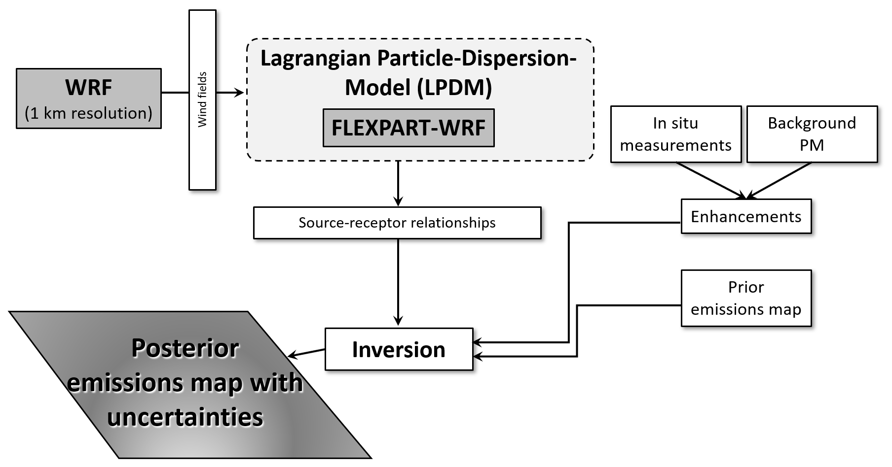
Figure 2Overview of the inverse model set-up, its inputs, and its outputs as used and described in this study.
As described above, given the meteorological input required to establish the source–receptor relationships, to estimate the PM emissions map, the inverse model must achieve a balance between the emphasis given to the prior emissions map and the PM concentration measurements. This balance is achieved by prescribing adequate uncertainty to the prior and to the measurements. For a single inversion performed, i.e. a posterior emissions map derived for a single time step, where a prior emissions map and a series of measurements are provided as input, the quality of the posterior emissions map (driven by the derived uncertainties) is likely to depend heavily on the quality of the prior emissions map, as reported by Guo et al. (2018), which is consistent with previous literature (e.g. Gurney et al., 2005; Lauvaux et al., 2016).
3.1 Transport modelling
In this study, the coupled LPDM FLEXPART–WRF model version 3.3.2 (Brioude et al., 2013) is used as the atmospheric transport model that relates changes in emissions to changes in concentrations, i.e. the source–receptor relationships (SRRs). FLEXPART-WRF combines the Weather Forecast and Research Model (WRF) version 4.0 (Skamarock et al., 2019) and the FLEXPART model (Stohl et al., 2005; Pisso et al., 2019) version 9.
3.1.1 Weather Research and Forecasting Model – WRF
A challenge for modelling PM dispersion in an urban environment is accurately representing the meteorological conditions and capturing, with high fidelity, the influence of terrain under complex topography on the meteorology (Fay and Neunhäuserer, 2006). For the purposes of this study, we use WRF (Skamarock et al., 2005), a widely used numerical weather prediction model designed for operational weather forecasting as well as atmospheric research.
WRF version 4.0 was employed to simulate the meteorological fields with four nested domains over Christchurch (Fig. A1). The model simulation set-up is describe in Appendix A1. Overall a total of 32 WRF simulations were performed, covering the period from 21 June to 18 July 2019. Each simulation was initialized daily at 00:00 UTC and ran for a total of 72 h, with the first 48 h allocated for spin up, which was discarded from the final output files that were used as input to FLEXPART-WRF. Furthermore, only the meteorological output from domain 4 (d04), spanning the latitude range from 44.05 to 43.25∘ S and longitude range from 172.29 to 173.4∘ E, with a horizontal resolution of 1 km (cf. 27, 9, and 3 km in Guo et al., 2018) and a temporal resolution of 10 min, was used as input to FLEXPART-WRF (Sect. 3.1.2).
Simulated temperatures and wind speed were compared to observations (Appendix A2), and it was found that while WRF has some difficulty in reproducing observed night-time temperatures during low-wind-speed conditions, WRF generally captures the meteorological conditions of the region within the typically expected uncertainties. For example, the overestimation of the wind speeds near the surface in the WRF model are a known feature of the model (e.g. Shimada et al., 2011), and uncertainties remain on whether this bias is caused only under specific conditions. Overall, we have confidence in the WRF model to use it as the driver for the dispersion model in the inversion formulation, using an appropriate characterization of the relevant uncertainties.
3.1.2 FLEXPART-WRF and footprint calculations
Using the meteorological output at a horizontal resolution of 1 km from WRF (Sect. 3.1.1 and Appendix A1) as input, FLEXPART-WRF was used to derive the source–receptor relationships (SSRs) by running the LPDM backward in time; e.g. particles were released from a measurement location to identify potential upwind sources. As the current version of FLEXPART-WRF does not support the direct simulation of PM2.5 concentrations, the FLEXPART-WRF simulation was set up to simulate the particles as passive tracer air parcels without considering chemical reactions and dry or wet deposition. To avoid the complications of wet deposition, we exclude rainy periods from our study (see below). The loss processes via chemistry and dry deposition were not considered as explained in the following.
-
Air chemistry in Christchurch in winter is such that there is little, if any, chemical transformation of PM because of the low background concentrations of sulfur dioxide (Coulson et al., 2016).
-
While loss through dry deposition is possible, it is unlikely to play a large role in Christchurch. There are no studies in Christchurch to confirm this assumption, but a study performed in California (Herner et al., 2006) under similar wintertime inversion conditions modelled deposition rates for particles of a size between 0.1 and 3 µm to be between and m s−1. During the evening hours when mixing depths are on the order of 50 m, these velocities suggest deposition timescales of 58 and 32 h. A study by Jeanjean et al. (2016) also found that deposition rates of PM2.5 are low, especially in winter.
Although these loss processes were not included in this study, we acknowledge potential small uncertainties to be introduced to the posterior emissions maps, which will also be acknowledged in Sect. 4. Future studies will need to consider the inclusion of these loss processes depending on the environment and PM2.5 sources in the city of interest.
To establish the SSR for each hourly mean PM measurement, FLEXPART-WRF simulations were initiated at the end of the 1 h period (noting that FLEXPART-WRF is running backward in time). Then, during the 1 min period, 10 000 particles were released continuously from 49 receptor locations that correspond to the measurement sites described in Sect. 2 and traced backwards in time over a 24 h period to establish their potential sources. The release altitude was set to 2 m for all releases, and the FLEXPART-WRF output was saved every 30 min on the same grid as the WRF output was provided, i.e. same domain with a 1 km horizontal resolution. Overall, FLEXPART-WRF was run independently for each hour of the 31 d spanning the period from 22 June to 18 July 2019.
FLEXPART-WRF output, provided in units of residence time (seconds), can be used to identify the origin of emissions sources that contribute to the concentrations “measured” at the receptor. We use the FLEXPART-WRF output to create “footprints” that describe the backwards-in-time local contributions to any in situ measurement by integrating over 12 h of output and over a 60 m thick surface layer. A time period of 12 h was chosen to be enough time for the particles to traverse the domain even under weak wind conditions, and 60 m was chosen as the integration height to be high enough to capture any elevated emissions sources. These footprints define the transport matrix (H), which is used to relate the emissions in flux space to the measurements in concentration space, as shown later in Eq. (1).
3.2 Prior PM2.5 emissions estimates
Derived bottom-up emissions estimates used in this study include PM2.5 emissions sources from (i) traffic, (ii) industry (the top 13 industries only), and (iii) home heating. At the time of this study, there was insufficient Christchurch-specific bottom-up data available to incorporate a temperature dependency into the prior; however we acknowledge that a robust handling of this could lead to improved posterior emissions estimates and should thus be considered in future investigations. Across the whole domain, home heating contributes 72 % to the total PM2.5 emissions on a typical winter day, while traffic and industry emissions only contribute 20 % and 8 % to the total emissions, respectively (Tim Mallett, ECan, personal communication 2020). The relatively high amount of emissions coming from home heating was a primary driver for the measurement campaign being conducted during the winter.
For this study, ECan provided an estimate for the average PM2.5 emission of a wood burner based on 2018 census data, issued permits for wood burners, and estimated emissions per burner type. It should be noted that ECan formulates their estimate with an eye towards the worst-case scenario, as this would be most relevant to negative human health impacts, and thus the prior emissions maps used here essentially act as the upper limit of estimated PM2.5 emissions.
The 2018 census data were compiled based on a set of questions taken to the Christchurch community regarding whether or not they used wood for home heating. The census data were provided on statistical areas, which are irregularly shaped polygons of various sizes covering the Christchurch city domain. To estimate the PM emissions from households in Christchurch, the number of households using a wood burner was multiplied by the average PM2.5 emissions per wood burner. Of these total household emissions, 73 % were then used as an estimate for PM2.5 emissions on a typical winter night. Here the assumption is that the type of wood burners and the percentage of active burners on a given night remain consistent across the city. The industry emissions for the top 13 emitters were calculated based on discharge estimates from ECan, and together they represent around 77 % of estimated industrial PM2.5 emissions for the Christchurch airshed. Vehicle emissions were also provided by ECan and are based on 2014 data from the Christchurch Transport Model, and emission factors were derived from the vehicle emissions prediction model that was developed by the New Zealand Transport Agency.
To derive hourly estimates of PM2.5 emissions, the total 24 h emissions were divided according to the estimated contribution of that hour to the total daily emissions for each of the three sources separately – these estimates were provided by ECan for home heating and traffic. Due to a lack of any detailed information about the timing of the emissions released by industries, it was assumed that the industry emissions were released evenly throughout the 24 h period. Overall the highest emissions occurred during nighttime when people were at home starting their fires.
The household-based emissions per statistical area and the traffic emissions were rasterized onto a 10 m by 10 m New Zealand Transverse Mercator 2000 (NZTM2000) grid. Industry emissions were added as point sources on this grid. During the rasterization, the conversion from grams per meshblock (statistical area) to grams per square metre was calculated. The NZTM2000 grid was interpolated and projected onto the fourth WRF domain (Fig. A1), using conservative interpolation which preserves the total emissions. The bottom-up estimate for PM2.5 emissions in Christchurch over a 24 h period is shown in Fig. 3, representing emissions on a typical winter day.
.
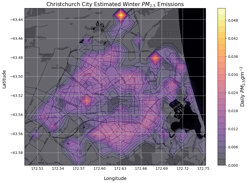
Figure 3Bottom-up emissions map over Christchurch, interpolated onto the 1 km WRF grid and used as the prior for the inversion calculation. PM2.5 emissions sources include (i) household heating, (ii) traffic, and (iii) industry. Contour lines are shown for every 0.002 g m−2 of PM2.5.
The hourly resolution maps are used to construct the final prior emissions map that is used in the Bayesian inversion equation. First, for any given hour with a given set of hourly measurements, the corresponding emissions map is a mean emissions map across the preceding 12 h of emissions. This averaging is done to match the 12 h length of the footprints, so that it is appropriately representative. Then, the definitive prior emissions map is a mean of each of these hourly emissions maps across every hour in the inversion period.
3.3 Determination of the background concentrations
Since this study focuses on constraining the emissions within the boundary of the city of Christchurch, the concentration measurements being provided as input to the inverse model should similarly only reflect the emissions coming from within the boundary of the city; i.e. they should exclude any contribution from emissions sources located outside the city. As a result, any potential influx of PM into the domain (here referred to as the background) needs to be subtracted off each concentration measurement taken within the city domain, leaving only concentrations that are a function of in-domain emissions, hereafter referred to as enhancements.
Defining the background air mass is often one of the most difficult yet important challenges during the inversion formulation (e.g. Göckede et al., 2010; Lauvaux et al., 2016). In the CO2 community, for example, this is often achieved by selecting a measurement site to act as a background based on wind direction (e.g. Kort et al., 2012; McKain et al., 2012; Lauvaux et al., 2016). Here, we adapted the approach to be applied to determine the background PM2.5 concentrations.
During the MAPM measurement campaign and to estimate the inflow of PM into the domain, several sensors were deployed on the perimeter of the city. Measurements from five of these “background” sites were used, together with wind direction measurements, to estimate the background PM concentrations flowing into the city. Specifically, the city of Christchurch was divided into four quadrants with Hagley Park at the centre. A total of five AWS–ODIN pairs were selected along the perimeter to determine the background PM concentrations. The five sites are marked in Fig. 1, as named sites. To determine whether or not the wind was blowing into the domain, the angle between the location of the AWS and Hagley Park was estimated. This angle corresponds to a wind direction under which air is being advected into the domain.
To estimate the background PM2.5 concentration at any given hour, 1 min resolution PM2.5 concentration measurements from the ODIN and 5 min resolution of the wind data were used in the following procedure.
-
For each AWS site, a range of wind direction angles were determined that correspond to the wind flowing into the domain (Table 1).
-
Using PM2.5 data from the ODIN corresponding to each AWS site, and the respective 5 min resolution wind data, we select all PM2.5 measurements that correspond to the range of wind directions that define air flowing into the domain.
-
For each site, the PM2.5 measurements that had been selected in the previous step were then screened for episodic short-term local emissions of PM based on (i) whether the change in PM2.5 from one minute to the next is greater than 50 µg m−3 and (ii) whether the PM2.5 measurement at time t exceeds 2σ, where σ is the standard deviation calculated from the 1 min data, for each hour of available measurements.
-
All remaining PM2.5 concentration measurements from all sites are combined into one time series and, because the temporal resolution of the concentration measurements used by the inverse model is hourly, hourly averages are calculated from these remaining measurements.
-
As a final step, and to remove any remaining local influences, a 10 d running median of the hourly time series is computed. This running median value is then used as the background PM2.5 concentration across the whole domain for a given hour of the day.
Table 1Wind direction angles that define air blowing into the city for each measurement site at the perimeter of the city.

Figure 4 shows a time series comparison of the adjusted background value against two of the measurement sites located near the centre of the city. These have been chosen to be ODIN sites SD0013 and SD0020. The new presented methodology has created a background time series that does not appear to contain any of the large spikes from stochastic local events, while still containing real, apparently reasonable background variations.
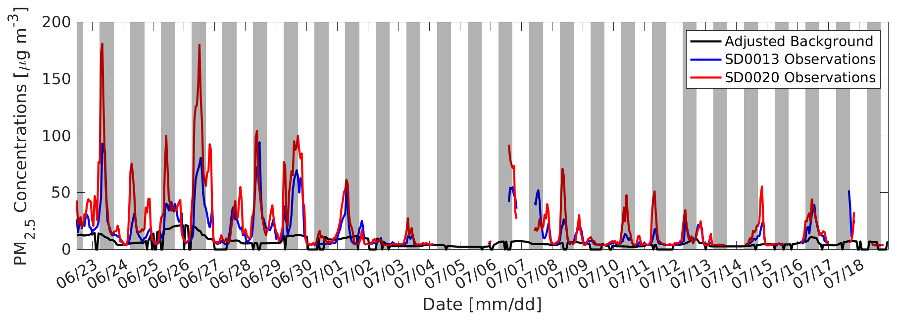
Figure 4A time series comparing the adjusted background value against two measurement sites located near the city centre.
3.4 Bayesian inversion calculation
Given the prior flux estimates of the emissions and the measured enhancements, the optimal emissions flux map is computed using the Bayesian inversion calculation, following the formula in Tarantola (2005):
Here, x is the posterior flux map, x0 is the prior flux map, B is the prior error covariance matrix, H is the influence function (more specifically the transport matrix, containing the 12 h footprints for each hourly measurement), R is the error covariance matrix for the observations, and y is the one-dimensional matrix of hourly averaged measured enhancements.
The posterior error matrix is defined as
The errors on the prior flux estimates are assigned in a manner similar to what has been described in Nathan et al. (2018) and Lauvaux et al. (2016). The error covariance matrix for the prior fluxes, B, contains the variances for every grid point in the domain along the diagonal and the cross-correlation terms in the off diagonals. The variances are defined as the square of the root mean square (rms) values at each grid point of the flux map, and the rms values are set to be 50 % of the corresponding flux value. The covariances, representing the spatial error correlations, are then defined using an exponential decay function with a 1 km correlation length. Here, we have set the correlation length to match the grid-cell size in the domain, to allow for more independence in the allocation of emissions adjustments during the inversion process. However, even with this near independence, we still maintain some spatial error correlations with the understanding that they are necessary to keep the inverse problem regularized and thus to prevent a divergence of the solution at points where the inverse model grid overlaps with the receptor sites, called the “colocalization problem” (Bocquet, 2005; Saide et al., 2011). To account for the possibility that the real structure of the error correlations is not properly captured by these additional spatial correlations, and that in fact we may be overestimating the correction, we do include some results without these spatial correlations later in Fig. 5. For the error covariance matrix for the observations, the variances are defined as the square of the measurement uncertainties that are provided with the data sets (Dale et al., 2021). The off-diagonal elements of the covariance matrix are all set to zero; i.e. all measurements at different locations and times are considered to be independent from one another.
An inversion calculation was performed using the measurements obtained during the MAPM field campaign (Sect. 2). The period for the inversion was chosen to be from 22 June 2019, 12:00 UTC to 18 July 2019, 24:00 UTC. The inversion was then run for the “daytime” and “nighttime” separately, where daytime was defined from 06:00 to 18:00 LT (18:00–06:00 UTC, excluding 06:00 UTC) and nighttime from 18:00 to 06:00 LT (06:00–18:00 UTC, excluding 18:00 UTC). One posterior map per day was computed for each daytime or nighttime period. The overall structure and components of the MAPM tool, including the inverse model system, are shown schematically in Fig. 2.
Because rain is known to wash out PM from the atmosphere (e.g. Atlas and Giam, 1988), which would lead to artificially low measurements and therefore would bias the inversion results, all hours during which rain occurred were removed from the data set. The 12 h following any rain event were also removed from the data set, to prevent over-counting in our inversion set-up which uses 12 h footprints; i.e. this allows the emissions to “build back up” enough in the atmosphere to match the 12 h integrated footprints that are used in this study. The “rainy hours” were identified by using data from the AWS that is installed close to the city centre, at Kyle Street (purple cross in Fig. 1), wherein any hour that recorded any nonzero precipitation value was deemed to indicate a potential rainfall event in the area during that hour. The PM2.5 measurements at that hour and the following 12 h for all PM measurements at all sites were thus excluded from the analysis.

Figure 5Time series of sum of the fluxes across the domain in the prior, posterior using a spatial correlation of 1 km, and posterior using no spatial correlation, for the daytime and nighttime inversions.
The results of the inversion indicate a significant overestimation of the inventory estimates for PM2.5 emissions in Christchurch. Figure 5 shows the time series comparison for prior-based flux estimates compared with the posterior flux estimates for the daytime and nighttime. The values shown are sums across the entire domain, for either the prior or posterior maps. The prior map at any hour is a mean of the preceding 12-hourly estimated emissions maps, a length that was chosen to correspond to the 12 h footprints for the measurements at that hour. A scale factor is derived for the creation of the corresponding “hourly” time series of posterior values, since only one posterior map is computed per daytime or nighttime period. This scale factor is defined as the proportion of the domain sum of the posterior emissions map divided by the domain sum of the mean prior emissions map (across all included hours) used in the inversion for the given daytime or nighttime period.
In addition, posterior emissions time series where (i) 1 km spatial correlation was included and (ii) no spatial correlation was considered in the construction of the prior uncertainty matrix are also shown in Fig. 5. As explained in Sect. 3.4, the inclusion of some non-zero spatial correlation value was implemented to address the “colocalization problem” that can lead to spurious corrections of the prior at grid cells where measurement sites are located (Bocquet, 2005). Furthermore, the tendency for residential areas to be in spatial proximity to each other gives some physical justification for the inclusion, in our problem, of a non-zero spatial correlation in the prior uncertainty matrix, as well. That said, we acknowledge that this is an imperfect metric to describe the system and that our description of the correlations may not adequately capture the complexity of the real situation. As a result, we include the dashed magenta line in Fig. 5 to show what the posterior results would be without the addition of this spatial correlation on the uncertainty. It shows that our system may be slightly overestimating the downward adjustment in the posterior emissions compared to the prior. However, this difference in the adjustment is small enough such as not to dramatically change the conclusions we draw from this analysis. For the remainder of the results section, we will thus present the results that are based on including a prior uncertainty matrix with a 1 km correlation length.
For both daytime and nighttime, the results indicate a 40 % to 60 % overestimation of the prior emissions compared to the posterior emissions. The impact of not including loss of PM due to chemistry and dry deposition may account for a small amount of this downward adjustment, as explained in Sect. 3.1.2. Rather, most of the observed posterior adjustment is believed to be an expected result following several assumptions that had been made when calculating the PM2.5 inventory (Tim Mallett from ECan, personal communication, October 2020) as follows.
-
A total of 73 % of wood burners are active on a typical night. The percentage was calculated from field surveys, where the “number of chimneys seen hot on a given night” was recorded, which was then divided by the respective number of households who reported using a wood burner to heat their home (obtained from census data). This results in the ratio of the number of wood burners active on a typical winter day.
-
The fuel use estimates assume around 10 h of use per day for wood burners. This can be an overestimation as (i) new homes have more insulation than previous houses; (ii) heat pumps are installed in new homes rather than wood burners, which lead to no PM emissions; and (iii) a smaller floor area or fewer occupants would reduce the burning time.
-
All wood burners over 1.0 g kg−1 are combined into one emission factor category, though a future version of the inventory separates out 1.0–1.5 g kg−1 from those over 1.5 g kg−1, which could further lower emissions estimates.
-
There is ambiguity in the underlying census data used to tally the number of active burners or the time they are used for, which only asks a homeowner whether they use a wood burner but does not include a question around whether or not they have an alternative heating method or an estimate of the average amount of time that they use the heating.
As a result, the inventory comes with a large uncertainty that favours the possibility of an overestimation. Thus, the results of the inverse model adjusting to lower emissions in the posterior, as in Fig. 5, is viewed as sensible. Recent observing system simulation experiments (OSSEs) presented by Lauvaux et al. (2020) indicate that an inversion set-up like the one used here should be able to recover values close to the true emissions if the prior fluxes are offset by as much as 20 %. However, large offsets above 40 % may not be able to be fully recovered and may still require an extra correction. In their study, a 40 % offset in the prior from the truth was still 18 % away from the truth after inversion. This may imply that the apparent overestimation in Christchurch's prior emissions is still larger than our posterior results indicate.
The nighttime period is traditionally left out of inversion analyses because of difficulties in the model to accurately capture the nocturnal boundary layer (Geels et al., 2007; Steeneveld et al., 2008). For example, Lac et al. (2013) found a positive bias of 5 ppm of CO2 in urban and suburban regions of Paris, which was attributed to a boundary layer height error in the transport model. Despite that, we are including the results from the nighttime inversion because the residuals for the nighttime analysis compared to the daytime analysis show overall good agreement, as seen in Fig. 5. Additionally, the nighttime is of particular interest to this investigation, as the primary source of PM2.5 emissions in Christchurch is home heating (Sect. 3.2), which is typically used in the evening when the ambient temperature is at its lowest. Thus, the results from the nighttime inversion are presented here as well, with the note that they should be accepted with caution.

Figure 6Example time series for in-city measurement sites showing the prior-based concentrations, the measured enhancements (i.e. PM2.5 concentration measurements where the background has been removed), and the posterior-based concentrations, showcasing the improvement provided by the inversion. Grey shaded areas indicate nighttime hours.
The nighttime posterior values inferred by the inversion and shown in Fig. 5 indicate generally more variable emissions from night to night compared to the results from the daytime inversions. Some of this variability can be explained in part to originate from the transport model uncertainty related to the nocturnal boundary layer height, as explained above. In general, however, the result present in the daytime inversions, i.e. that the posterior estimates are significantly lower than the corresponding priors, is upheld.
We also acknowledge the presence of some negative emissions values in some grid cells of the posterior. This may occur in situations where the observed enhancement values for the city are made negative due to the uncertainties inherent in an imperfect background characterization, as is the case during the daytime inversion for 26 June. However, negative pixels may also naturally result simply from the analytical solution to the Bayesian inversion equation we implement. This is also the case in our situation, yet we would consider the implementation of a positivity constraint to be an unjustifiable manipulation to the mathematical system. As a result, the mean posterior grid for the daytime inversions contains 28 negative pixels out of the 9100 total, and the mean nighttime posterior grid contains 29 negative pixels out of the 9100 total. These negative pixels comprise such a small proportion of the domain that they are not considered to materially change our conclusions. Rather, we make note of them here in the interest of transparency.
Figure 6 shows two time series plots from measurement sites towards the centre of the domain (near the city centre). By multiplying the prior or posterior flux maps by the transport operator H, we can compare the prior and posterior estimates against the measurements directly in concentration space. Then, for any given measurement site, these time series can be plotted. By noting where the red line (posterior estimates) matches the measurements (black line) better than the blue line (prior estimates), we see the adjustments by the inversion at this measurement site.
In general, the concentrations derived from the posterior converge from the prior concentrations towards the measured enhancements, which indicates that the inversion is working insofar as the uncertainty on the measurements is much smaller than that on the prior fluxes, and therefore the measurements have a strong influence on the posterior result. The model has difficulty with capturing some of the strong spike events seen in the measurements, especially during nighttime, but overall it is able to follow the general variability seen in the enhancement time series, across all instruments (Fig. 6). The events of high PM2.5 concentrations correspond to periods of low wind speeds and low temperatures. However, these enhancements could also be the result of a local source, which either is not well-resolved by the inverse model due to the comparatively coarse 1 km resolution or is a consequence of having instruments positioned too close to the surface.
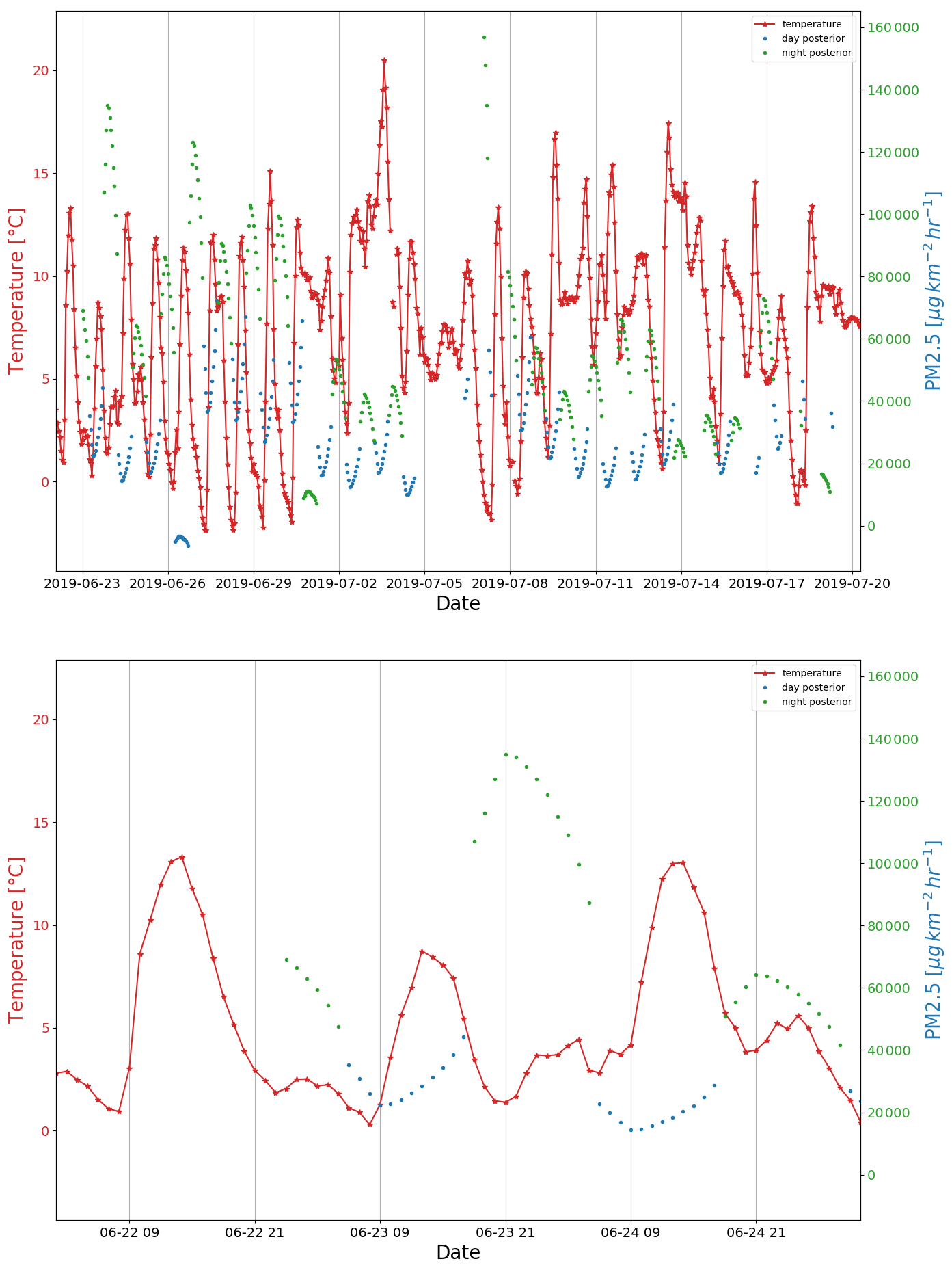
Figure 7Hourly mean temperature as obtained from the AWS located at Kyle Street, together with the sum of the inferred PM2.5 emissions for daytime (blue) and nighttime (green).
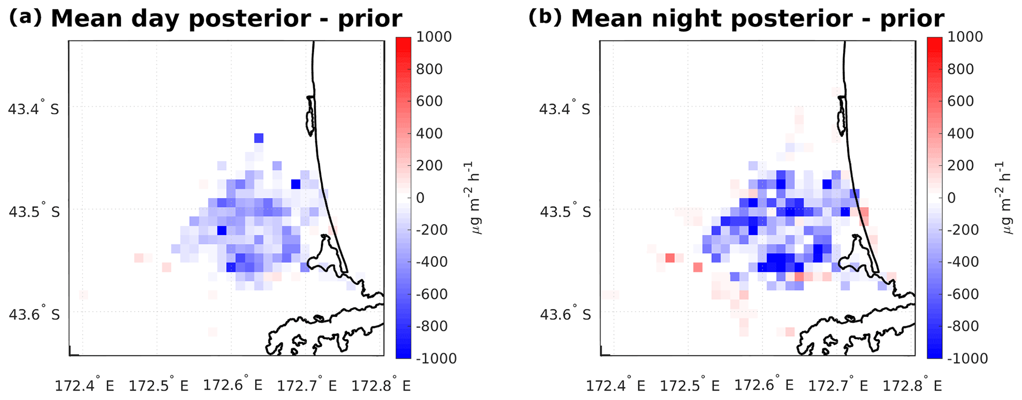
Figure 8The mean difference between the posterior and prior maps in the daytime (a) and nighttime (b) across the full inversion period. The mean prior and posterior were calculated from the 10 daytime and nighttime maps, respectively.
Figure 7 takes a broader look at the temperature relationship of the system, showing the temperature time series obtained from an AWS located near the city centre (Kyle Street) plotted together with the sum of the daytime and nighttime posterior emissions. The top panel shows this comparison across the entire analysis period, while the bottom panel shows a zoom-in of a particular period. The posterior emissions are, as expected, anti-correlated with temperature; i.e. during nighttime when the temperature is low, the emissions increase and vice versa. This is consistent with the primary driver of emissions in Christchurch being the use of wood burners. Also, during warm periods, e.g. between 2 and 5 July, while following a diurnal cycle, the emissions are rather low, reflecting that the use of wood burners was reduced during that period. These results give us confidence that the inverse model is producing reasonable results.
To understand where the adjustments are being made spatially, we include maps of the mean difference between the posterior and the prior over the course of the analysis period, for both daytime and nighttime, as shown in Fig. 8. The correction for apparent overestimates in the prior is distributed throughout the city during both day and night. Also, several of the large point sources present in the prior (see the Fig. 3), have had many of the corrections attributed to them. This is a consequence, in part, of the flux uncertainty scaling with the prior emissions, as the inversion will preferentially attribute corrections to grid points with large uncertainties. Since the overwhelming majority of emissions are expected to come from home heating, it can be assumed that a large majority of the corrections may apply to that sector. However that does not rule out the possibility of misattributions in other factors of the prior, as well (e.g. traffic and industry).
Furthermore, the results reveal an apparent increase in emissions in a ring just outside of the city, especially during nighttime. Given that these areas outside of the city had fewer measurement sites nearby, and thus fewer footprints overlapping the regions with which to issue corrections, it is possible that these sites are simply reflecting under-representation in the model. This may be evidenced by the fact that these effects are amplified at night, where the transport error is at its highest due to the difficulties with accurately simulating the nocturnal boundary layer. However, it is also possible that these are real sources of emissions that are not well-captured and identified by the inventory because of, for example, new developments that may have been built after the information for the construction of the prior was gathered in 2018.
The results of the presented study are considered to provide an improved estimation of the quantity and distribution of PM2.5 emissions from the region during the wintertime 2019 measurement campaign. However, the study still contains several substantial sources of uncertainty that may have affected the results and should therefore be acknowledged. Although they have been identified throughout this paper, we restate them here for clarity and transparency. First, the low sampling heights for the majority of the instruments (46 % of instruments at or below 3 m above the ground) open the door for local turbulence to have impacted the measurements; future studies should make every effort to record measurements at higher altitudes. Furthermore, the modelled atmospheric transport always involves some potentially impactful amount of uncertainty. Beyond the characterized mismatches with the winds, a future study could become more robust by including in situ measurements of the boundary layer, as well. Additionally, the characterization of the inflow, used to define the background PM2.5 values across the measurement stations at any particular hour, can be a significant source of uncertainty, as well. Further, it is expected that the loss processes are only contributing a small uncertainty to the inferred emissions maps for Christchurch during winter; however, the decision to not explicitly account for loss processes (specifically chemical or dry deposition, as discussed in Sect. 3.1.2) will need to be given thorough reconsideration in any future applications of the methodology described here for cities other than Christchurch.
The PM2.5 inversion system established through the MAPM project using Christchurch, New Zealand, as its test bed has been shown to be an effective system for assessing aerosol emissions in the urban environment using a large number of measurement sites. The system was applied to measurements obtained during the MAPM field campaign during the winter of 2019.
The inversion results suggest what appears to be a systematic overestimation in the prior emissions estimates of PM2.5 for Christchurch, which is in the range of 40 %–60 %, but which may be higher due to limitations of the inverse calculation in situations with such a large mismatch. This conclusion is in line with what would be expected, considering several of the assumptions that had been used in the calculation of the inventory on which the prior emissions estimate is based. The fact that the prior emissions estimate was created with an eye towards a worst-case scenario, to err on the side of caution for human health, means that an overestimation of some significance would have been expected. Site comparisons against the measurements in concentration space appear to give further support to the idea that the inversion is capturing the real trends seen in the measured enhancement data.
The presented results constitute a proof-of-concept study for inferring PM emissions sources on a city scale, using Christchurch as a test bed for high-measurement-density aerosol urban inversions, to provide city officials with near-real-time assessments of surface emissions. We successfully demonstrate the feasibility of the system, and our investigation has itself identified potential areas of improvement in the current emissions estimates for Christchurch. This study lays the groundwork for future investigations that may seek the same goal in disparate urban environments around the globe.
We assessed the different sources of uncertainty inherent in our approach. One of the largest areas is the transport model. Thus, the logical next step is going to be to implement a higher-resolution model that can better characterize wind flows and turbulence at urban scales: the PArallelized Large-eddy simulation Model (PALM; Maronga et al., 2015). This will be coupled to WRF and, eventually, will include chemistry in the model to capture the effects of aerosol chemistry and deposition. The coupled WRF–PALM system, which has been developed by Lin et al. (2020), will be better able to simulate air flow (including, for example, effects of turbulence and diffusivity) in complex urban terrains and would provide higher-resolution output (10 m or finer, compared to the current 1 km resolution).
We have additional ideas that could improve future efforts to implement MAPM more robustly, as well. First, such investigations may benefit from developing a more robust prior that incorporates some temperature dependency, especially if again being implemented in an area where wood burners are the primary source of wintertime PM2.5 emissions. Additionally, future efforts focused outside of Christchurch may need to more explicitly handle secondary organic aerosols in the transport model.
A1 Model simulations performed with WRF
The numerical weather prediction model WRF version 4.0 was used to provide meteorological fields that were used as input to FLEXPART-WRF. The model was run for four nested domains with horizontal resolutions of 27, 9, 3, and 1 km and 38 vertical levels, as shown in Fig. A1. The European Centre for Medium-Range Weather Forecasts (ECMWF) reanalysis data – ERA5 (Hersbach et al., 2020) with a horizontal resolution of 0.25∘ and 137 model levels at 3-hourly time resolution were used as the boundary and initial conditions. The WRF sea surface temperatures (SSTs) were initialized from the daily National Centers for Environmental Prediction (NCEP) high-resolution SST analysis (0.083∘). The CONUS physics suite (Liu et al., 2017) was selected for all the domains, which contains parameterizations for micro-physics, radiation, planetary boundary layer, surface layer, land surface, and cumulus. Due to the high horizontal resolution of the final two domains (d03 and d04), the cumulus parameterization was turned off for these domains. The standard high-resolution static data were used for these simulations.
A2 WRF evaluation against observations
Temperature, wind speed, and direction, as simulated by WRF, were compared to measurements made using AWSs at seven different locations in and surrounding Christchurch. The 2 m temperature and 10 m wind speed from WRF were interpolated using a bi-linear interpolation to the latitude and longitude location of each AWS measurement site, forming a time series for comparison. The seven AWS sites, whose locations are marked in Fig. 1, measured wind speed at various heights ranging from 2 to 6 m. To make these measurements comparable to the 10 m wind that is provided by WRF, the measured wind speeds were raised to 10 m using a log wind profile with a roughness length of z0=0.3 m, which corresponds to a terrain with scattered obstacles.
Modelled and measured temperature, wind speed and direction are shown in Fig. A2 for the period 28 June to 5 July 2019. During periods of low wind speed (e.g. 28–30 June), WRF accurately simulates the temperature during the day but overestimated the 2 m temperature by up to 9∘ at night. This bias is not apparent on other days when the wind speed is higher. This suggests that WRF may have difficulty accurately simulating the temperature inversion layers that form in winter within the boundary layer, causing the surface temperatures to be overestimated by WRF. On warmer days and on days with higher wind speeds, WRF represents the measured temperature and wind direction at Kyle Street well, while it overestimates measured wind speeds. During the inversion period (22 June–18 July) the difference between 10 min mean AWS wind speed measured at Kyle Street and the location-interpolated wind speed hindcast simulated by WRF was less than 1 m s−1 53 % of the time and less than 2 m s−1 81 % of the time.
The local topography may have an impact on the performance of WRF, as well. For example, the nighttime temperature biases for the downtown Kyle Street station, presented in Fig. A2, were the most extreme observed, and corresponding nighttime temperatures hindcast by WRF at several other AWS sites were also often several degrees warmer than was observed by the AWSs. However, this effect was not observed at the Mt Sugarloaf site, which is located atop a peak in the Port Hills at an altitude of 494 m. This is considered to be a consequence of the station height being above the height of many of the temperature inversion layers that form. Wind speed at the Sugarloaf site was also generally underestimated by a large margin. This is also unsurprising, as the wind flows at this site will be dependent on the surrounding complex topography that fall below the spatial resolution of the WRF model.
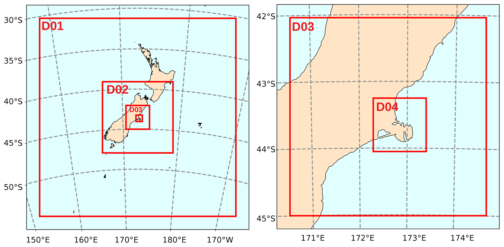
Figure A1WRF domain configuration: (left) domains d01 and d02 with a horizontal resolution of 27 000 m and 9000 m, respectively, and (right) domains d03 and d04 with a horizontal resolution of 3000 and 1000 m, respectively. Figure adapted from Lin et al. (2020).
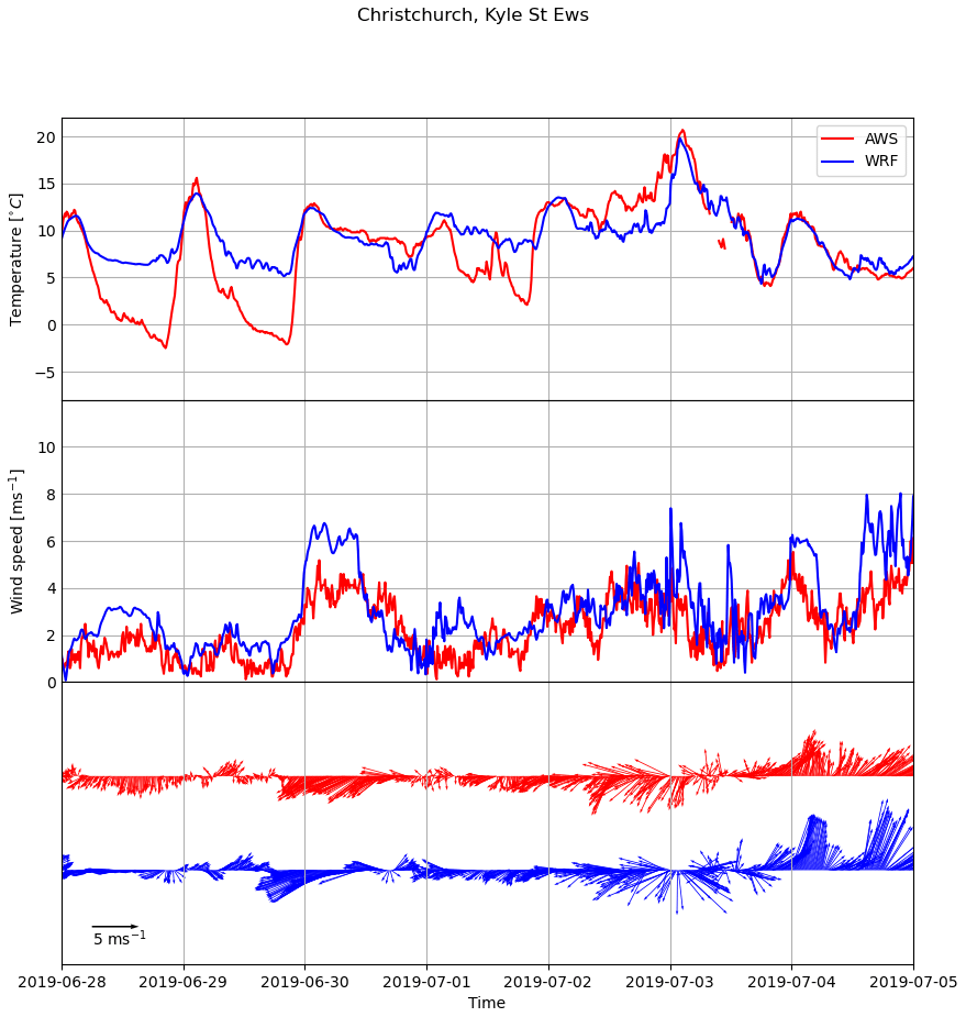
Figure A2Example time series of 2 m temperature, 10 m wind speed, and wind direction measured by the AWS installed at Kyle Street, compared to the temperature, wind speed, and direction as simulated by WRF between 28 June and 5 July 2019.
The MATLAB code for the inverse model described in this paper is hosted on GitHub, and access can be obtained from the corresponding author.
The PM data collected during the MAPM field campaign are publicly available from https://doi.org/10.5281/zenodo.4023693 (Dale et al., 2020). AWS data that were collected by the permanently installed AWSs are available from NIWA (https://cliflo.niwa.co.nz/, NIWA, 2021) or the New Zealand MetService.
BN wrote much of the inverse model code and wrote much of the paper together with input from all co-authors. SK assisted with writing of the paper, performed the FLEXPART-WRF simulations, and participated in the discussions around the inverse model set-up and results. SMF managed the inverse model development and set-up and provided critical input throughout the project regarding its set-up, feedback on which analyses to perform and how to present them, and edits for the paper. GB wrote some sub-sections of the paper and copy-edited other sections of the paper. LB generated the bottom-up emissions map based on census data and participated in the discussions around the inverse model results. LB and DL performed the WRF simulations that were used in this study, while ED performed the comparison of the WRF output to observations. ED provided all PM and AWS measurements used in this study. GO and ES performed the uncertainty analysis on the measurements.
The authors declare that they have no conflict of interest.
Publisher's note: Copernicus Publications remains neutral with regard to jurisdictional claims in published maps and institutional affiliations.
We acknowledge the New Zealand Ministry of Business, Innovation & Employment (MBIE) for funding the MAPM project. We additionally acknowledge Guy Coulson and Ian Longley from NIWA in Auckland, New Zealand, for their time and efforts contributing to this project, particularly in treating the measurement data. We further acknowledge Tim Mallett from Environment Canterbury for his assistance with the creation of what became the prior emissions maps, as well as his insight and contextualization of our results. We acknowledge Basit Khan from KIT in Garmisch-Partenkirchen, Germany, and Marwan Katurji from the University of Canterbury for providing their constructive advice on setting up WRF simulations and interpreting the simulation results. We also acknowledge Thomas Lauvaux for his expert insights into some of the specific behaviours of our inversion system, including with some technical help to appropriately address some reviewer concerns. Finally, we acknowledge Beata Bukosa from NIWA in Wellington, New Zealand, who attended the regular (near-weekly) progress/update meetings and joined in the discussion or offered her perspective at several points throughout the process.
This research has been supported by the Ministry of Business, Innovation & Employment (MBIE, grant no. BSCIF1802).
This paper was edited by Markus Petters and reviewed by Peter Rayner and one anonymous referee.
Adams, K., Greenbaum, D. S., Shaikh, R., van Erp, A. M., and Russell, A. G.: Particulate matter components, sources, and health: Systematic approaches to testing effects, JAPCA J. Air Waste Ma., 65, 544–558, https://doi.org/10.1080/10962247.2014.1001884, 2015. a
Anderson, J. O., Thundiyil, J. G., and Stolbach, A.: Clearing the Air: A Review of the Effects of Particulate Matter Air Pollution on Human Health, Journal of Medical Toxicology, 8, 166–175, https://doi.org/10.1007/s13181-011-0203-1, 2012. a
Atlas, E. and Giam, C.: Ambient concentration and precipitation scavenging of atmospheric organic pollutants, Water Air Soil Poll., 38, 19–36, 1988. a
Bocquet, M.: Grid resolution dependence in the reconstruction of an atmospheric tracer source, Nonlin. Processes Geophys., 12, 219–233, https://doi.org/10.5194/npg-12-219-2005, 2005. a, b
Bréon, F. M., Broquet, G., Puygrenier, V., Chevallier, F., Xueref-Remy, I., Ramonet, M., Dieudonné, E., Lopez, M., Schmidt, M., Perrussel, O., and Ciais, P.: An attempt at estimating Paris area CO2 emissions from atmospheric concentration measurements, Atmos. Chem. Phys., 15, 1707–1724, https://doi.org/10.5194/acp-15-1707-2015, 2015. a
Brioude, J., Arnold, D., Stohl, A., Cassiani, M., Morton, D., Seibert, P., Angevine, W., Evan, S., Dingwell, A., Fast, J. D., Easter, R. C., Pisso, I., Burkhart, J., and Wotawa, G.: The Lagrangian particle dispersion model FLEXPART-WRF version 3.1, Geosci. Model Dev., 6, 1889–1904, https://doi.org/10.5194/gmd-6-1889-2013, 2013. a, b
Bulot, F. M. J., Johnston, S. J., Basford, P. J., Easton, N. H. C., Apetroaie-Cristea, M., Foster, G. L., Morris, A. K. R., Cox, S. J., and Loxham, M.: Long-term field comparison of multiple low-cost particulate matter sensors in an outdoor urban environment, Sci. Rep., 9, 7497, https://doi.org/10.1038/s41598-019-43716-3, 2019. a
Castro, P., Velarde, M., Ardao, J., Perlado, M., and Sedano, L. A.: Validation of Real Time Dispersion of Tritium over the Western Mediterranean Basin in Different Assessments, Fusion Sci. Technol., 61, 355–360, https://doi.org/10.13182/FST12-A13445, 2012. a
Chevallier, F., Ciais, P., Conway, T. J., Aalto, T., Anderson, B. E., Bousquet, P., Brunke, E. G., Ciattaglia, L., Esaki, Y., Fröhlich, M., Gomez, A., Gomez-Pelaez, A. J., Haszpra, L., Krummel, P. B., Langenfelds, R. L., Leuenberger, M., MacHida, T., Maignan, F., Matsueda, H., Morguí, J. A., Mukai, H., Nakazawa, T., Peylin, P., Ramonet, M., Rivier, L., Sawa, Y., Schmidt, M., Steele, L. P., Vay, S. A., Vermeulen, A. T., Wofsy, S., and Worthy, D.: CO2 surface fluxes at grid point scale estimated from a global 21 year reanalysis of atmospheric measurements, J. Geophys. Res.-Atmos., 115, 1–17, https://doi.org/10.1029/2010JD013887, 2010. a
Contini, D. and Costabile, F.: Does Air Pollution Influence COVID-19 Outbreaks?, Atmosphere, 11, 377, https://doi.org/10.3390/atmos11040377, 2020. a
Coulson, G., Olivares, G., and Talbot, N.: Aerosol Size Distributions in Auckland, Air Quality and Climate Change, 50, 23–28, https://doi.org/10.3316/informit.931019171837291, 2016. a, b
Coulson, G., Somervell, E., Mitchell, E., Longley, I., and Olivares, G.: Ten years of woodburner research in New Zealand: A review, Air Quality and Climate Change, 51, 59–67, 2017. a
Crinnion, W.: Particulate Matter Is a Surprisingly Common Contributor to Disease, Integrative medicine (Encinitas, Calif.), 16, 8–12, 2017. a
Dale, E., Kremser, S., Tradowsky, J., Bodeker, G., Bird, L., Olivares, G., Coulson, G., Somervell, E., Pattinson, W., Barte, J., and Schmidt, J.-N.: MAPM Campaign PM Data, Zenodo [data set], https://doi.org/10.5281/zenodo.4023693, 2020. a
Dale, E. R., Kremser, S., Tradowsky, J. S., Bodeker, G. E., Bird, L. J., Olivares, G., Coulson, G., Somervell, E., Pattinson, W., Barte, J., Schmidt, J.-N., Abrahim, N., McDonald, A. J., and Kuma, P.: The winter 2019 air pollution (PM2.5) measurement campaign in Christchurch, New Zealand, Earth Syst. Sci. Data, 13, 2053–2075, https://doi.org/10.5194/essd-13-2053-2021, 2021. a, b, c, d, e
Dominici, F., Peng, R. D., Bell, M. L., Pham, L., McDermott, A., Zeger, S. L., and Samet, J. M.: Fine particulate air pollution and hospital admission for cardiovascular and respiratory diseases, JAMA-J. Am. Med. Assoc., 295, 1127–1134, https://doi.org/10.1001/jama.295.10.1127, 2006. a
Enting, I.: Inverse Problems in Atmospheric Constituent Transport, Cambridge University Press, New York, 2002. a
Fattorini, D. and Regoli, F.: Role of the chronic air pollution levels in the Covid-19 outbreak risk in Italy, Environ. Pollut., 264, 114 732, https://doi.org/10.1016/j.envpol.2020.114732, 2020. a
Fay, B. and Neunhäuserer, L.: Evaluation of high-resolution forecasts with the non-hydrostaticnumerical weather prediction model Lokalmodell for urban air pollutionepisodes in Helsinki, Oslo and Valencia, Atmos. Chem. Phys., 6, 2107–2128, https://doi.org/10.5194/acp-6-2107-2006, 2006. a
Gariazzo, C., Papaleo, V., Pelliccioni, A., Calori, G., Radice, P., and Tinarelli, G.: Application of a Lagrangian particle model to assess the impact of harbour, industrial and urban activities on air quality in the Taranto area, Italy, Atmos. Environ., 41, 6432–6444, https://doi.org/10.1016/j.atmosenv.2007.06.005, 2007. a
Geels, C., Gloor, M., Ciais, P., Bousquet, P., Peylin, P., Vermeulen, A. T., Dargaville, R., Aalto, T., Brandt, J., Christensen, J. H., Frohn, L. M., Haszpra, L., Karstens, U., Rödenbeck, C., Ramonet, M., Carboni, G., and Santaguida, R.: Comparing atmospheric transport models for future regional inversions over Europe – Part 1: mapping the atmospheric CO2 signals, Atmos. Chem. Phys., 7, 3461–3479, https://doi.org/10.5194/acp-7-3461-2007, 2007. a
Gentner, D. R., Ford, T. B., Guha, A., Boulanger, K., Brioude, J., Angevine, W. M., de Gouw, J. A., Warneke, C., Gilman, J. B., Ryerson, T. B., Peischl, J., Meinardi, S., Blake, D. R., Atlas, E., Lonneman, W. A., Kleindienst, T. E., Beaver, M. R., Clair, J. M. St., Wennberg, P. O., VandenBoer, T. C., Markovic, M. Z., Murphy, J. G., Harley, R. A., and Goldstein, A. H.: Emissions of organic carbon and methane from petroleum and dairy operations in California's San Joaquin Valley, Atmos. Chem. Phys., 14, 4955–4978, https://doi.org/10.5194/acp-14-4955-2014, 2014. a
Göckede, M., Turner, D. P., Michalak, A. M., Vickers, D., and Law, B. E.: Sensitivity of a subregional scale atmospheric inverse CO2 modeling framework to boundary conditions, J. Geophys. Res.-Atmos., 115, 1–15, https://doi.org/10.1029/2010JD014443, 2010. a
Guo, L., Chen, B., Zhang, H., Xu, G., Lu, L., Lin, X., Kong, Y., Wang, F., and Li, Y.: Improving PM2.5 Forecasting and Emission Estimation Based on the Bayesian Optimization Method and the Coupled FLEXPART-WRF Model, Atmosphere, 9, 428, https://doi.org/10.3390/atmos9110428, 2018. a, b, c, d
Gurney, K. R., Law, R. M., Denning, A. S., Rayner, P. J., Baker, D., Bousquet, P., Bruhwiler, L., Chen, Y. H., Clals, P., Fan, S., Fung, I. Y., Gloor, M., Heimann, M., Higuchi, K., John, J., Maki, T., Maksyutov, S., Masarie, K., Peylin, P., Prather, M., Pak, B. C., Randerson, J., Sarmiento, J., Taguchi, S., Takahashi, T., and Yuen, C. W.: Towards robust regional estimates of CO2 sources and sinks using atmospheric transport models, Nature, 415, 626–630, https://doi.org/10.1038/415626a, 2002. a
Gurney, K. R., Chen, Y. H., Maki, T., Kawa, S. R., Andrews, A., and Zhu, Z.: Sensitivity of atmospheric CO2 inversions to seasonal and interannual variations in fossil fuel emissions, J. Geophys. Res.-Atmos., 110, 1–13, https://doi.org/10.1029/2004JD005373, 2005. a
Hegarty, J., Draxler, R. R., Stein, A. F., Brioude, J., Mountain, M., Eluszkiewicz, J., Nehrkorn, T., Ngan, F., and Andrews, A.: Evaluation of Lagrangian Particle Dispersion Models with Measurements from Controlled Tracer Releases, J. Appl. Meteorol. Clim., 52, 2623–2637, https://doi.org/10.1175/JAMC-D-13-0125.1, 2013. a
Herner, J. D., Ying, Q., Aw, J., Gao, O., Chang, D. P. Y., and Kleeman, M. J.: Dominant Mechanisms that Shape the Airborne Particle Size and Composition Distribution in Central California, Aerosol Sci. Tech., 40, 827–844, https://doi.org/10.1080/02786820600728668, 2006. a
Hersbach, H., Bell, B., Berrisford, P., Hirahara, S., Horányi, A., Muñoz-Sabater, J., Nicolas, J., Peubey, C., Radu, R., Schepers, D., Simmons, A., Soci, C., Abdalla, S., Abellan, X., Balsamo, G., Bechtold, P., Biavati, G., Bidlot, J., Bonavita, M., De Chiara, G., Dahlgren, P., Dee, D., Diamantakis, M., Dragani, R., Flemming, J., Forbes, R., Fuentes, M., Geer, A., Haimberger, L., Healy, S., Hogan, R. J., Hólm, E., Janisková, M., Keeley, S., Laloyaux, P., Lopez, P., Lupu, C., Radnoti, G., de Rosnay, P., Rozum, I., Vamborg, F., Villaume, S., and Thépaut, J.-N.: The ERA5 global reanalysis, Q. J. Roy. Meteor. Soc., 146, 1999–2049, https://doi.org/10.1002/qj.3803, 2020. a
Jeanjean, A., Monks, P., and Leigh, R.: Modelling the effectiveness of urban trees and grass on PM2.5 reduction via dispersion and deposition at a city scale, Atmos. Environ., 147, 1–10, https://doi.org/10.1016/j.atmosenv.2016.09.033, 2016. a
Kort, E. A., Frankenberg, C., Miller, C. E., and Oda, T.: Space-based observations of megacity carbon dioxide, Geophys. Res. Lett., 39, L17806, https://doi.org/10.1029/2012GL052738, 2012. a
Lac, C., Donnelly, R. P., Masson, V., Pal, S., Riette, S., Donier, S., Queguiner, S., Tanguy, G., Ammoura, L., and Xueref-Remy, I.: CO2 dispersion modelling over Paris region within the CO2-MEGAPARIS project, Atmos. Chem. Phys., 13, 4941–4961, https://doi.org/10.5194/acp-13-4941-2013, 2013. a
Lauvaux, T., Miles, N. L., Deng, A., Richardson, S. J., Cambaliza, M. O., Davis, K. J., Gaudet, B., Gurney, K. R., Huang, J., O'Keefe, D., Song, Y., Karion, A., Oda, T., Patarasuk, R., Razlivanov, I., Sarmiento, D., Shepson, P., Sweeney, C., Turnbull, J., and Wu, K.: High resolution atmospheric inversion of urban CO2 emissions during the dormant season of the Indianapolis Flux Experiment (INFLUX), J. Geophys. Res.-Atmos., 121, 5213–5236, https://doi.org/10.1002/2015JD024473, 2016. a, b, c, d, e
Lauvaux, T., Gurney, K. R., Miles, N. L., Davis, K. J., Richardson, S. J., Deng, A., Nathan, B. J., Oda, T., Wang, J. A., Hutyra, L., and Turnbull, J.: Policy-relevant assessment of urban CO2emissions, Environ. Sci. Technol., 54, 10237–10245, https://doi.org/10.1021/acs.est.0c00343, 2020. a
Lin, D., Khan, B., Katurji, M., Bird, L., Faria, R., and Revell, L. E.: WRF4PALM v1.0: a mesoscale dynamical driver for the microscale PALM model system 6.0, Geosci. Model Dev., 14, 2503–2524, https://doi.org/10.5194/gmd-14-2503-2021, 2021. a, b
Lin, J. C., Gerbig, C., Wofsy, S. C., Andrews, A. E., Daube, B. C., Davis, K. J., and Grainger, C. A.: A near-field tool for simulating the upstream influence of atmospheric observations: The Stochastic Time-Inverted Lagrangian Transport (STILT) model, J. Geophys. Res.-Atmos., 108, 4493, https://doi.org/10.1029/2002JD003161, 2003. a
Liu, C., Ikeda, K., Rasmussen, R., Barlage, M., Newman, A. J., Prein, A. F., Chen, F., Chen, L., Clark, M., Dai, A., Dudhia, J., Eidhammer, T., Gochis, D., Gutmann, E., Kurkute, S., Li, Y., Thompson, G., and Yates, D.: Continental-scale convection-permitting modeling of the current and future climate of North America, Clim. Dynam., 49, 71–95, https://doi.org/10.1007/s00382-016-3327-9, 2017. a
Maksyutov, S., Oda, T., Saito, M., Janardanan, R., Belikov, D., Kaiser, J. W., Zhuravlev, R., Ganshin, A., Valsala, V. K., Andrews, A., Chmura, L., Dlugokencky, E., Haszpra, L., Langenfelds, R. L., Machida, T., Nakazawa, T., Ramonet, M., Sweeney, C., and Worthy, D.: Technical note: A high-resolution inverse modelling technique for estimating surface CO2 fluxes based on the NIES-TM–FLEXPART coupled transport model and its adjoint, Atmos. Chem. Phys., 21, 1245–1266, https://doi.org/10.5194/acp-21-1245-2021, 2021. a
Mallett, T.: Air quality status report Christchurch airshed, Environement Canterbury, Regional Council, Rep. no. R14/116, ISBN 978-0-908316-38-0, 2014. a
Maronga, B., Gryschka, M., Heinze, R., Hoffmann, F., Kanani-Sühring, F., Keck, M., Ketelsen, K., Letzel, M. O., Sühring, M., and Raasch, S.: The Parallelized Large-Eddy Simulation Model (PALM) version 4.0 for atmospheric and oceanic flows: model formulation, recent developments, and future perspectives, Geosci. Model Dev., 8, 2515–2551, https://doi.org/10.5194/gmd-8-2515-2015, 2015. a
McKain, K., Wofsy, S. C., Nehrkorn, T., Eluszkiewicz, J., Ehleringer, J. R., and Stephens, B. B.: Assessment of ground-based atmospheric observations for verification of greenhouse gas emissions from an urban region., P. Natl. Acad. Sci. USA, 109, 8423–8, https://doi.org/10.1073/pnas.1116645109, 2012. a
Nathan, B. J., Lauvaux, T., Turnbull, J. C., Richardson, S. J., Miles, N. L., and Gurney, K. R.: Source Sector Attribution of CO2 Emissions Using an Urban Bayesian Inversion System, J. Geophys. Res., 123, 13611–13621, https://doi.org/10.1029/2018JD029231, 2018. a
Pisso, I., Sollum, E., Grythe, H., Kristiansen, N. I., Cassiani, M., Eckhardt, S., Arnold, D., Morton, D., Thompson, R. L., Groot Zwaaftink, C. D., Evangeliou, N., Sodemann, H., Haimberger, L., Henne, S., Brunner, D., Burkhart, J. F., Fouilloux, A., Brioude, J., Philipp, A., Seibert, P., and Stohl, A.: The Lagrangian particle dispersion model FLEXPART version 10.4, Geosci. Model Dev., 12, 4955–4997, https://doi.org/10.5194/gmd-12-4955-2019, 2019. a, b
NIWA: New Zealand's National Climate Database, CliFlo, [data set], available at: https://cliflo.niwa.co.nz/, last access: 10 September 2021. a
Saide, P., Bocquet, M., Osses, A., and Gallardo, L.: Constraining surface emissions of air pollutants using inverse modelling: method intercomparison and a new two-step two-scale regularization approach, Tellus B, 63, 360–370, https://doi.org/10.1111/j.1600-0889.2011.00529.x, 2011. a
Scott, A. and Sturman, A.: Beyond emission inventories: tracking the main sources of airborne PM in Christchurch, New Zealand, Clean Air and Environmental Quality, 40, 35–42, 2006. a
Seibert, P. and Frank, A.: Source-receptor matrix calculation with a Lagrangian particle dispersion model in backward mode, Atmos. Chem. Phys., 4, 51–63, https://doi.org/10.5194/acp-4-51-2004, 2004. a
Shimada, S., Ohsawa, T., Chikaoka, S., and Kozai, K.: Accuracy of the Wind Speed Profile in the Lower PBL as Simulated by the WRF Model, SOLA, 7, 109–112, https://doi.org/10.2151/sola.2011-028, 2011. a
Skamarock, W. C., Klemp, J. B., Dudhia, J., Gill, D. O., Barker, D. M., Wang, W., and Powers, J. G.: A description of the advanced research WRF version 2, no. NCAR/TN-468+STR, https://doi.org/10.5065/D6DZ069T, report available at: https://opensky.ucar.edu/islandora/object/technotes:479 (last access: 30 November 2020), 2005. a
Skamarock, W. C., Klemp, J. B., Dudhia, J., Gill, D. O., Liu, Z., Berner, J., Wang, W., Powers, J. G., Duda, M. G., Barker, D. M., and Huang, X.-Y.: A description of the advanced research WRF Model version 4, National Center for Atmospheric Research: Boulder, CO, USA, p. 145, available at: https://opensky.ucar.edu/islandora/object/technotes:576/datastream/PDF, (last access: 30 November 2020), 2019. a
Steeneveld, G. J., Mauritsen, T., De Bruijn, E. I., and Vilà-Guerau de Arellano, J.: Evaluation of limited-area models for the representation of the diurnal cycle and contrasting nights in CASES-99, J. Appl. Meteorol. Clim., 47, 869–887, https://doi.org/10.1175/2007JAMC1702.1, 2008. a
Stein, A. F., Draxler, R. R., Rolph, G. D., Stunder, B. J. B., Cohen, M. D., and Ngan, F.: NOAA's HYSPLIT Atmospheric Transport and Dispersion Modeling System, B. Am. Meteorol. Soc., 96, 2059–2077, https://doi.org/10.1175/BAMS-D-14-00110.1, 2016. a
Stohl, A., Hittenberger, M., and Wotawa, G.: Validation of the lagrangian particle dispersion model FLEXPART against large-scale tracer experiment data, Atmos. Environ., 32, 4245–4264, https://doi.org/10.1016/S1352-2310(98)00184-8, 1998. a
Stohl, A., Forster, C., Frank, A., Seibert, P., and Wotawa, G.: Technical note: The Lagrangian particle dispersion model FLEXPART version 6.2, Atmos. Chem. Phys., 5, 2461–2474, https://doi.org/10.5194/acp-5-2461-2005, 2005. a, b, c
Tarantola, A.: Inverse Problem Theory and Methods for Model Parameter Estimation, Society for Industrial and Applied Mathematics, Siam, 2005. a
Tinarelli, G., Anfossi, D., Brusasca, G., Ferrero, E., Giostra, U., Morselli, M., Moussafir, J., Trombetti, F., and Tampieri, F.: Lagrangian particle simulation of tracer dispersion in the lee of a schematic two-dimensional hill, J. Appl. Meteorol., 33, 744–756, 1994. a
Trini Castelli, S., Armand, P., Tinarelli, G., Duchenne, C., and Nibart, M.: Validation of a Lagrangian particle dispersion model with wind tunnel and field experiments in urban environment, Atmos. Environ., 193, 273–289, https://doi.org/10.1016/j.atmosenv.2018.08.045, 2018. a
Tunno, B., Longley, I., Somervell, E., Edwards, S., Olivares, G., Gray, S., Cambal, L., Chubb, L., Roper, C., Coulson, G., and Clougherty, J. E.: Separating spatial patterns in pollution attributable to woodsmoke and other sources, during daytime and nighttime hours, in Christchurch, New Zealand, Environ Res, 171, 228–238, https://doi.org/10.1016/j.envres.2019.01.033, 2019. a
Turner, A. J., Shusterman, A. A., McDonald, B. C., Teige, V., Harley, R. A., and Cohen, R. C.: Network design for quantifying urban CO2 emissions: assessing trade-offs between precision and network density, Atmos. Chem. Phys., 16, 13465–13475, https://doi.org/10.5194/acp-16-13465-2016, 2016. a
Turner, A. J., Kim, J., Fitzmaurice, H., Newman, C., Worthington, K., Chan, K., Wooldridge, P. J., Köehler, P., Frankenberg, C., and Cohen, R. C.: Observed Impacts of COVID-19 on Urban CO2 Emissions, Geophys. Res. Lett., 47, e2020GL090 037, https://doi.org/10.1029/2020GL090037, 2020. a
Wu, X., Nethery, R. C., Sabath, M. B., Braun, D., and Dominici, F.: Air pollution and COVID-19 mortality in the United States: Strengths and limitations of an ecological regression analysis, Science Advances, 6, eabd4049, https://doi.org/10.1126/sciadv.abd4049, 2020. a
Zanobetti, A., Franklin, M., Koutrakis, P., and Schwartz, J.: Fine particulate air pollution and its components in association with cause-specific emergency admissions, Environ. Health-Glob., 8, 58, https://doi.org/10.1186/1476-069X-8-58, 2009. a
Zheng, T., Bergin, M. H., Johnson, K. K., Tripathi, S. N., Shirodkar, S., Landis, M. S., Sutaria, R., and Carlson, D. E.: Field evaluation of low-cost particulate matter sensors in high- and low-concentration environments, Atmos. Meas. Tech., 11, 4823–4846, https://doi.org/10.5194/amt-11-4823-2018, 2018. a
Zhu, Y., Xie, J., Huang, F., and Cao, L.: Association between short-term exposure to air pollution and COVID-19 infection: Evidence from China, Sci. Total Environ., 727, 138 704, https://doi.org/10.1016/j.scitotenv.2020.138704, 2020. a
- Abstract
- Introduction
- MAPM measurement campaign
- Inverse modelling framework
- Inversion calculation using measurements obtained during the MAPM field campaign
- Conclusions
- Appendix A
- Code availability
- Data availability
- Author contributions
- Competing interests
- Disclaimer
- Acknowledgements
- Financial support
- Review statement
- References