Heterogeneity and chemical reactivity of the remote troposphere defined by aircraft measurements

The NASA Atmospheric Tomography (ATom) mission built a photochemical climatology of air parcels based on in situ measurements with the NASA DC-8 aircraft along objectively planned profiling transects through the middle of the Pacific and Atlantic oceans. In this paper we present and analyze a data set of 10 s (2 km) merged and gap-filled observations of the key reactive species driving the chemical budgets of O₃ and CH₄ (O₃, CH₄, CO, H₂O, HCHO, H₂O₂, CH₃OOH, C₂H₆, higher alkanes, alkenes, aromatics, NO_x, HNO₃, HNO₄, peroxyacetyl nitrate, other organic nitrates), consisting of 146 494 distinct air parcels from ATom deployments 1 through 4. Six models calculated the O₃ and CH₄ photochemical tendencies from this modeling data stream for ATom 1. We find that 80 %–90 % of the total reactivity lies in the top 50 % of the parcels and 25 %–35 % in the top 10 %, supporting previous model-only studies that tropospheric chemistry is driven by a fraction of all the air. In other words, accurate simulation of the least reactive 50 % of the troposphere is unimportant for global budgets. Surprisingly, the probability densities of species and reactivities averaged on a model scale (100 km) differ only slightly from the 2 km ATom data, indicating that much of the heterogeneity in tropospheric chemistry can be captured with current global chemistry models. Comparing the ATom reactivities over the tropical oceans with climatological statistics from six global chemistry models, we find excellent agreement with the loss of O₃ and CH₄ but sharp disagreement with production of O₃. The models sharply underestimate O₃ production below 4 km in both Pacific and Atlantic basins, and this can be traced to lower NO_x levels than observed. Attaching photochemical reactivities to measurements of chemical species allows for a richer, yet more constrained-to-what-matters, set of metrics for model evaluation.

1 Prologue

This paper is based on the methods and results of papers that established an approach for analyzing aircraft measurements, specifically the NASA Atmospheric Tomography Mission (ATom), with global chemistry models. Here we present a brief overview of those papers to help the reader understand the basis for this paper. The first ATom modeling paper (“Global atmospheric chemistry – which air matters”, Prather et al., 2017, hence P2017) gathered six global models, both chemistry–transport models (CTMs) and chemistry–climate models (CCMs). The models reported a single-day snapshot for mid-August (the time of the first ATom deployment, ATom-1), and these included all species relevant for tropospheric chemistry and the 24 h reactivities. We limited our study to three reactivities (Rs) controlling methane (CH₄) and tropospheric ozone (O₃) using specific reaction rates to define the loss of CH₄ and the production and loss of O₃ in parts per billion (ppb) per day. The critical photolysis rates (J values) are also reported as 24 h averages.

$$\begin{array}{}\text{(1)}& \text{L-CH4}:{\mathrm{CH}}_{\mathrm{4}}+\mathrm{OH}\to {\mathrm{CH}}_{\mathrm{3}}+{\mathrm{H}}_{\mathrm{2}}\mathrm{O}\left(\mathrm{1}\right)\end{array}$$

$$\begin{array}{}\text{(2a)}& {\displaystyle }& {\displaystyle }\text{P-O3}:{\mathrm{HO}}_{\mathrm{2}}+\mathrm{NO}\to {\mathrm{NO}}_{\mathrm{2}}+\mathrm{RO}\text{(2b)}& {\displaystyle }& {\displaystyle }{\mathrm{RO}}_{\mathrm{2}}+\mathrm{NO}\to {\mathrm{NO}}_{\mathrm{2}}+\mathrm{RO},\text{(2c)}& {\displaystyle }& {\displaystyle }\text{where}{\mathrm{NO}}_{\mathrm{2}}+h\mathit{\nu }\to \mathrm{NO}+\text{O and O}+{\mathrm{O}}_{\mathrm{2}}\to {\mathrm{O}}_{\mathrm{3}}\text{(2d)}& {\displaystyle }& {\displaystyle }{\mathrm{O}}_{\mathrm{2}}+h\mathit{\nu }\to \text{O}+\text{O}\left(x\mathrm{2}\right)\end{array}$$

$$\begin{array}{}\text{(3a)}& {\displaystyle }& {\displaystyle }\text{L-O3}:{\mathrm{O}}_{\mathrm{3}}+\mathrm{OH}\to {\mathrm{O}}_{\mathrm{2}}+{\mathrm{HO}}_{\mathrm{2}}\text{(3b)}& {\displaystyle }& {\displaystyle }{\mathrm{O}}_{\mathrm{3}}+{\mathrm{HO}}_{\mathrm{2}}\to \mathrm{HO}+{\mathrm{O}}_{\mathrm{2}}+{\mathrm{O}}_{\mathrm{2}}\text{(3c)}& {\displaystyle }& {\displaystyle }\mathrm{O}{(}^{\mathrm{1}}\mathrm{D})+{\mathrm{H}}_{\mathrm{2}}\mathrm{O}\to \mathrm{OH}+\mathrm{OH}\end{array}$$

$$\begin{array}{}\text{(4)}& {\displaystyle }& {\displaystyle }\text{J-O1D}:{\mathrm{O}}_{\mathrm{3}}+h\mathit{\nu }\to \mathrm{O}{(}^{\mathrm{1}}\mathrm{D})+{\mathrm{O}}_{\mathrm{2}}\text{(5)}& {\displaystyle }& {\displaystyle }\text{J-NO2}:{\mathrm{NO}}_{\mathrm{2}}+h\mathit{\nu }\to \mathrm{NO}+\mathrm{O}\end{array}$$

Models also reported the change in O₃ over 24 h, and these match the P-O3 minus L-O3 values over the Pacific basin (a focus of this study). The models showed a wide range in the three Rs average profiles across latitudes over the Pacific basin, as well as 2D probability densities (PDs) for key species such as NO_x (NO + NO₂) versus HOOH. A large part of the model differences was attributed to the large differences found in chemical composition. We found that single transects from a model through the tropical Pacific at different longitudes produced nearly identical 2D PDs, but these PDs were distinctly different across models. This result supported the premise that the ATom PDs would provide a useful metric for global chemistry models.

In P2017, we established a method for running the chemistry modules in the CTMs and CCMs with an imposed chemical composition from aircraft data: the ATom run, or “A run”. In the A run, the chemistry of each grid cell does not interact with its neighbors or with externally imposed emission sources. Effectively the CTM/CCM is initialized and run for 24 h without transport, scavenging or emissions. Aerosol chemistry is also turned off in the A runs. This method allows each parcel to evolve in response to the daily cycle of photolysis in each model and be assigned a 24 h integrated reactivity. The instantaneous reaction rates at the time an air parcel is measured (e.g., near sunset at the end of a flight) do not reflect that parcel's overall contribution to the CH₄ or O₃ budget; a full diel cycle is needed. The A run assumption that parcels do not mix with neighboring air masses is an approximation, and thus for each model we compared the A runs using the model's restart data with a parallel standard 24 h simulation (including transport, scavenging, and emissions). Because the standard grid-cell air moves and mixes, we compared averages over a large region (e.g., tropical Pacific). We find some average biases of order ±10 % but general agreement. The largest systematic biases in the A runs are caused by buildup of HOOH (no scavenging) and decay of NO_x (no sources). The A runs are relatively easy to code for most CTM/CCMs and allow each model's chemistry module, including photolysis package, to run normally. The A runs do not distinguish between CTMs and CCMs, except that each model will generate/prescribe its own cloud fields and photolysis rates. Our goal is to create a robust understanding of the chemical statistics including the reactivities with which to test and evaluate the free-running CCMs, and thus we do not try to model the specific period of the ATom deployments. Others may use the ATom data with hindcast CTMs to test forecast models, but here we want to build a chemical climatology.

The first hard test of the A runs came with the second ATom modeling paper (“How well can global chemistry models calculate the reactivity of short-lived greenhouse gases in the remote troposphere, knowing the chemical composition”, Prather et al., 2018, hence P2018). The UCI CTM simulated an aircraft-like data set of 14 880 air parcels along the International Date Line from a separate high-resolution (0.5^∘) model. Each parcel is defined by the following core species: H₂O, O₃, NO_x, HNO₃, HNO₄, PAN (peroxyacetyl nitrate), CH₃NO₃, HOOH, CH₃OOH, HCHO, CH₃CHO (acetaldehyde), C₃H₆O (acetone), CO, CH₄, C₂H₆, alkanes (C₃H₈ and higher), C₂H₄, aromatics (benzene, toluene, xylene) and C₅H₈ (isoprene), plus temperature. Short-lived radicals (e.g., OH, HO₂, CH₃OO) were initialized at small concentrations and quickly reached daytime values determined by the core species. The six CTM/CCMs overwrote the chemical composition of a restart file, placing each pseudo-observation in a unique grid cell according to its latitude, longitude, and pressure. If another parcel is already in that cell, then it is shifted east–west or north–south to a neighboring model cell. For coarse-resolution models, multiple restart files and A runs were used to avoid large location shifts. CTM/CCMs usually have a locked in 24 h integration step starting at 00:00 UTC that is extremely difficult to modify in order to try to match the local solar time of observation, especially as it changes along aircraft flights. We tested the results with a recoded UCI CTM to start at 12:00 UTC but retain the same clouds fields over the day and found only percentage-level differences between a midnight or noon start.

These A runs averaged over cloud conditions by simulating 5 d in August at least 5 d apart. Assessment of the modeled photolysis rates and comparison with the ATom-measured J values is presented in Hall et al. (2018, hence H2018). All models agreed that a small fraction of chemically hot air parcels in the synthetic data set controlled most of the total reactivity. Some models had difficulty in implementing the A runs because they overwrote the specified water vapor with the modeled value, but this problem is fixed here. In both P2017 and P2018, the GISS-E2 model stood out with the most unusual chemistry patterns and sometimes illogical correlations. Efforts by a co-author to clarify the GISS results or identify errors in the implementation have not been successful. GISS results are included here for completeness in the set of three papers but are not reconciled. Overall, three models showed remarkable inter-model agreement in the three Rs with less than half of the RMSD (root-mean-square difference) as compared with the other models. UCI also tested the effect of different model years (1997 and 2015 versus reference year 2016), which varies the cloud cover and photolysis rates, and found an inter-year RMSD about half of that of the core model's RMSD. Thus, there is a fundamental uncertainty in this approach due to the inability to specify the cloud/photolysis history seen by a parcel over 24 h, but it is less than the inter-model differences among the most similar models.

2 Introduction

The NASA Atmospheric Tomography (ATom) mission completed a four-season deployment, each deployment flying from the Arctic to Antarctic and back, traveling south through the middle of the Pacific Ocean, across the Southern Ocean and then north through the Atlantic Ocean, with near-constant profiling of the marine troposphere from 0.2 to 12 km altitude (see Fig. S1 in the Supplement). The DC8 was equipped with in situ instruments that documented the chemical composition and conditions at time intervals ranging from < 1 to about 100 s (Wofsy et al., 2018). ATom measured hundreds of gases and aerosols, providing information on the chemical patterns and reactivity in the vast remote ocean basins, where most of the destruction of tropospheric ozone (O₃) and methane (CH₄) occurs. Reactivity is defined here as in P2017 to include the production and loss of O₃ (P-O3 and L-O3, ppb/d) and loss of CH₄ (L-CH4, ppb/d). Here we report on this model-derived product that was proposed for ATom, the daily averaged reaction rates determining the production and loss of O₃ and the loss of CH₄ for 10 s averaged air parcels. We calculate these rates with 3D chemical models that include variations in clouds and photolysis and then assemble the statistical patterns describing the heterogeneity (i.e., high spatial variability) of these rates and the underlying patterns of reactive gases.

Tropospheric O₃ and CH₄ contribute to climate warming and global air pollution (Stocker et al., 2013). Their abundances in the troposphere are controlled largely by tropospheric chemical reactions. Thus, chemistry–climate assessments seeking to understand past global change and make future projections for these greenhouse gases have focused on the average tropospheric rates of production and loss and how these reactivities are distributed in large semi-hemispheric zones throughout the troposphere (Griffiths et al., 2021; Myhre et al., 2014; Naik et al., 2013; Prather et al., 2001; Stevenson et al., 2006, 2013, 2020; Voulgarakis et al., 2013; Young et al., 2013). The models used in these assessments disagree on these overall CH₄ and O₃ reactivities (a.k.a. the budgets), and resolving the cause of such differences is stymied because of the large number of processes involved and the resulting highly heterogeneous distribution of chemical species that drive the reactions. Simply put, the models use emissions, photochemistry and meteorological data to generate the distribution of key species such as nitrogen oxides (NO_x= NO + NO₂) and hydrogen peroxide (HOOH) (step 1) and then calculate the CH₄ and O₃ reactivities from these species (step 2). There is no single average measurement that can test the verisimilitude of the models. Stratospheric studies such as Douglass et al. (1999) have provided a quantitative basis for testing chemistry and transport and defining model errors, but few of these studies have tackled the problem of modeling the heterogeneity of tropospheric chemistry. The major model differences lie in the first step because when we specify the mix of key chemical species, most models agree on the CH₄ and O₃ chemical budgets (P2018). The intent of ATom was to collect an atmospheric sampling of all the key species and the statistics defining their spatial variability and thus that of the reactivities of CH₄ and O₃.

Many studies have explored the ability of chemistry–transport models (CTMs) to resolve finer scales such as pollution layers (Eastham and Jacob, 2017; Rastigejev et al., 2010; Tie et al., 2010; Young et al., 2018; Zhuang et al., 2018), but these have not had the chemical observations (statistics) to evaluate model performance. In a great use of chemical statistics, Yu et al. (2016) used 60 s data (∼ 12 km) from the SEAC⁴RS aircraft mission to compare cumulative probability densities (PDs) of NO_x, O₃, HCHO and isoprene over the Southeast US with the GEOS-Chem CTM run at different resolutions. They identified clear biases at the high and low ends of the distribution, providing a new test of models based on the statistics rather than mean values. Heald et al. (2011) gathered high-resolution profiling of organic and sulfate aerosols from 17 aircraft missions and calculated statistics (mean, median, quartiles) but only compared with the modeled means. The HIAPER Pole-to-Pole Observations (HIPPO) aircraft mission (Wofsy, 2011) was a precursor to ATom with regular profiling of the mid-Pacific including high-frequency 10 s sampling that identified the small scales of variability throughout the troposphere. HIPPO measurements were limited in species, lacking O₃, NO_x and many of the core species needed for reactivity calculations. ATom, with a full suite of reactive species and profiling through the Atlantic basin, provides a wealth of chemical statistics that challenge the global chemistry models.

Our task here is the assembly of the modeling data stream (MDS), which provides flight-wise continuous 10 s data (air parcels) for the key reactive species. The MDS is based on direct observations and interpolation methods to fill gaps as documented the Supplement. Using the MDS, we have six chemical models calculating the 24 h reactivities, producing a reactivity data stream (RDS) using protocols noted in the Prologue (P2017) and described further in Sect. 2. There, we describe the updated modeling protocol RDS^* necessary to address measurement noise in key species that can be very short-lived. In Sect. 4, we examine the statistics of reactivity over the Atlantic and Pacific oceans, focusing on air parcels with high reactivity; for example, 10 % of the parcels produce 25 %–35 % of total reactivity over the oceans. We compare these ATom-1 statistics, species and reactivities with August climatologies from six global chemistry models. In one surprising result, ATom-1 shows a more reactive tropical troposphere than found in most models' climatologies associated with higher NO_x levels than in the models. Section 5 concludes that the ATom PDs based on 10 s air parcels do provide a valid chemistry metric for global models with 1^∘ resolution. It also presents some examples where ATom measurements and modeling can test the chemical relationships and may address the cause of differences in the O₃ and CH₄ budgets currently seen across the models. With this paper we release the full ATom MDS-2 from all four deployments, along with the updated RDS^* reactivities from the UCI model.

3 Models and data

3.1 The modeling data stream (MDS)

The ATom mission was designed to collect a multi-species, detailed chemical climatology that documents the spatial patterns of chemical heterogeneity throughout the remote troposphere. Figure S1 in the Supplement maps the 48 research flights, and the Supplement has tables summarizing each flight. We required a complete set of key species in each air parcel to initialize the models that calculate the CH₄ and O₃ reactivities. We choose the key reactive species (H₂O, O₃, CO, CH₄, NO_x, PSSNO_x (photostationary state NO_x), HNO₃, HNO₄, PAN, CH₂O, H₂O₂, CH₃OOH, acetone, acetaldehyde, C₂H₆, C₃H₈, i-C₄H₁₀, n-C₄H₁₀, alkanes, C₂H₄, alkenes, C₂H₂, C₅H₈, benzene, toluene, xylene, CH₃ONO₂, C₂H₅ONO₂, RONO₂, CH₃OH) directly from the ATom measurements and then add corollary species or other observational data indicative of industrial or biomass burning pollution or atmospheric processing (HCN, CH₃CN, SF₆, relative humidity, aerosol surface area (four modes) and cloud indicator). We choose 10 s averages for our air parcels as a compromise and because the 10 s merged data are a standard product (Wofsy et al., 2018). A few instruments measure at 1 s intervals, but the variability at this scale is not that different from 10 s averages (Fig. S2). Most of the key species are reported as 10 s values, with some being averaged or sampled at 30 s or longer such as ∼ 90 s for some flask measurements.

Throughout ATom, gaps occur in individual species on a range of timescales due to calibration cycles, sampling rates or instrument malfunction. The generation of the MDS uses a range of methods to fill these gaps and assigns a flag index to each species and data point to allow users to identify primary measurements and methods used for gap-filling. Where two instruments measure the same species, the MDS selects a primary measurement and identifies which instrument was used with a flag. The methodology and species-specific information on how the current MDS version 2 (MDS-2) is constructed, plus statistics on the 48 research flights and the 146 494 10 s air parcels in MDS-2, are given in the Supplement.

Over the course of this study, several MDS versions were developed and tested, including model-derived RDSs from these versions, some of which are used in this paper. In early ATom science team meetings, there was concern about the accuracy of NO₂ direct measurements when at very low concentrations. A group prepared an estimate for NO_x using the NO and O₃ measurements to calculate a photostationary value for NO₂ and thus NO_x. This PSS-NO_x became the primary NO_x source in version 0 (i.e., MDS-0). The numbering of versions initially followed the notation of revisions in the mission data archive (MDS_R0, MDS_R1, …), but this was restrictive, and we adopted the simpler notation here but still beginning with version 0. With MDS-0, we chose to gap-fill using correlations with CO to estimate the variability of the missing measurement over the gap. The science team then rejected PSS-NO_x as a proxy, and we reverted to the observed NO + NO₂ for MDS-1, resulting in increased NO_x and reactivities (RDS-1). MDS-1 NO_x values are 25 % larger on average than MDS-0 values (unweighted mean of 66 vs. 52 ppt), and this affects P-O3 most and L-CH4 least. We then estimated errors in the gap-filling and found that CO had little skill as a proxy for most other species. With MDS-2, we optimized and tested the treatments of gap-filling and lower limit of detection, along with other quality controls. MDS-2 is fully documented in the Supplement.

3.2 The reactivity data stream (RDS)

The concept of using an MDS to initialize 3D global chemistry models and calculate an RDS was developed in the pre-ATom methodology papers (P2017; P2018). In this paper, we use the original six models for their August chemical statistics, and we use five of them plus a box model to calculate the reactivities; see Table 1. The RDS is really a protocol applied to the MDS. It is introduced in the Prologue, and the details can be found in P2018. A model grid cell is initialized with all the core reactive species needed for a regular chemistry simulation. The model is then integrated over 24 h without transport or mixing, without scavenging and without emissions. Each global model uses its own varying cloud fields for the period to calculate photolysis rates, but the F0AM box model simply takes the instant J values as measured on the flight and applies a diurnal scaling. We can initialize with the core species and let the radicals (OH, HO₂, RO₂) come into photochemical balance. The 24 h integration is not overly sensitive to the start time of the integration, and thus models do not have to synchronize with the local time of observation (see P2018's Fig. S8 and Table S8).

Table 1 Chemistry models.

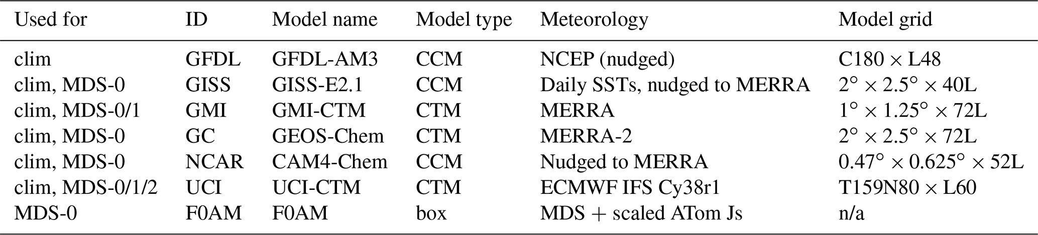
The descriptions of models used in the paper. The first column denotes if the model's August climatology is used (“clim”) and also the MDS versions used. F0AM used chemical mechanism MCMv331 plus J-HNO₄ plus O¹D)+CH₄. For the global models, see P2017, P2017 and H2018. n/a – not applicable

The initial RDS came from MDS-0 and six of the models in Table 1. This paper was nearly complete when we identified the problem with PSS-NO_x. We had gathered enough information on how models agree, or disagree, with RDS-0 and thus chose to assess MDS-1 with two of the models that closely agreed (GMI and UCI). The two models were very close in RDS-0 and also in RDS-1. We then found the problems with the CO proxy and chose to use only the UCI model as a transfer standard for the change from MDS-1 to MDS-2 (i.e., RDS-1 to RDS-2). This path avoided much extra work by the modeling groups and generated the same information on cross-model differences and a robust estimate of changes from RDS-0 to RDS-2.

Statistics for the three reactivities for six models using MDS-0, 2 alternative UCI model years using MDS-0, the GMI model using MDS-1 and the UCI model using MDS-2 are given in Tables 2 and S8 for three domains: global (all points), Pacific (oceanic data from 54^∘ S to 60^∘ N) and Atlantic (same constraints as Pacific). UCI MDS-1 is similar to UCI MDS-2 and is not shown. The statistics try to achieve equal latitude-by-pressure sampling by weighting each ATom parcel inversely according to the number of parcels in each 10^∘ latitude by 100 hPa bin. We calculate the means and medians plus the percent of total reactivity in the top 10 % of the weighted parcels (Table 2) and also the mean reactivity of the top 10 %, percent of total reactivity in the top 50 %, 10 % and 3 % plus the mean J values (Table S8).

Unfortunately, while investigating sensitivities and uncertainties in the RDS for a future study, we found an inconsistency between the reported concentrations of both pernitric acid (HNO₄) and peroxyacetyl nitrate (PAN) with respect to the chemical kinetics used in the models. High concentrations (attributed to instrument noise) were reported under conditions where the thermal decomposition frequency was > 0.4 per hour in the lower troposphere (> 253 K for HNO₄ and > 291 K for PAN). Thus, these species instantly become NO_x. There is no easy fix for this, and we left the species data in the MDS as they were reported but developed a new protocol RDS^* to deal with them. Both species are allowed to decay for 24 h using their thermal decomposition rate before being put into the model. This avoids most of the fast thermal release of NO_x in the 24 h of the RDS calculation but does not affect the release of NO_x from photolysis or OH reactions in the upper troposphere where thermal decomposition in inconsequential. It is possible that some of the high concentrations of HNO₄ and PAN in the lower troposphere are real and that we are missing this large source of NO_x with the RDS^* protocol, but there are no obvious sources of these species in the remote oceanic regions that would produce enough to match the thermal loss. Both this problem and its solution do not affect the initial NO_x. This revised protocol (UCI2^*) is shown in Tables 2 and S8 next to the standard protocol (UCI2). The reactivities drop slightly (3 % for P-O3, 2 % for L-O3 and 0 % for L-CH4) as expected with less NO_x, but the sensitivity of the reactivities to these compounds ($\partial \ln R/\partial \ln X$) drops by a factor of 2 or more. We use the UCI2^* results as our best estimate of the ATom reactivities for the figures in this paper.

Table 2 Reactivity statistics for the three large domains (global, Pacific, Atlantic).

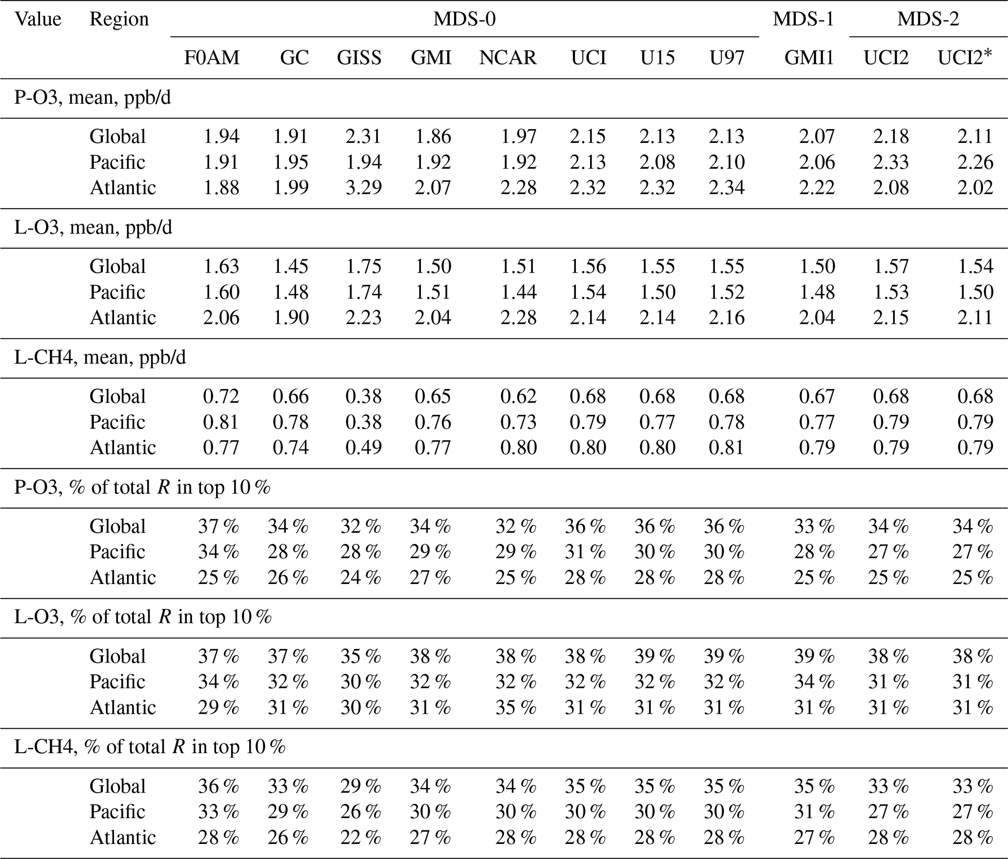
Global includes all ATom-1 parcels, Pacific considers all measurements over the Pacific Ocean from 54^∘ S to 60^∘ N and Atlantic uses parcels from 54^∘ S to 60^∘ N over the Atlantic basin. All parcels are weighted inversely by the number of parcels in each 10^∘ latitude by 100 hPa bin. Results from the different MDS versions (0, 1, 2) are shown. UCI2^* uses the revised RDS^* protocol that preprocesses the MDS-2 initializations with a 24 h decay of HNO₄ and PAN according to their local thermal decomposition frequencies; see text. See additional statistics in Table S8.

3.3 Inter-model differences

Variations in reactivities due to clouds are an irreducible source of uncertainty: predicting the cloud-driven photolysis rates that a shearing air parcel will experience over 24 h is not possible here. The protocol uses 5 separated 24 h days to average over synoptically varying cloud conditions. The standard deviation (σ) of the 5 d, as a percentage of the 5 d mean, is averaged over all parcels and shown in Table S9 for the five global models. Three central models (GC, GMI, UCI) show 9 %–10 % σ(Js) values and similar σ(Rs) values as expected if the variation in J values is driving the reactivities. Two models (GISS, NCAR) have 12 %–17 % σ(Js), which might be explained by more opaque clouds, but the amplified σ(R) values (14 %–32 %) are inexplicable. This discrepancy needs to be resolved before using these two models for ATom RDS analysis.

Inter-model differences are shown in the parcel-by-parcel root-mean-square (rms) differences for RDS-0 in Table 3. Even when models adopt standard kinetic rates and cross sections (i.e., Burkholder et al., 2015), the number of species and chemical mechanisms included, as well as the treatment of families of similar species or intermediate short-lived reaction products, varies across models. For example, UCI considers about 32 reactive gases, whereas GC and GMI have over 100, and F0AM has more than 600. The other major difference across models is photolysis, with models having different cloud data and different methods for calculating photolysis rates in cloudy atmospheres (H2018). The three central models (GC, GMI, UCI) in terms of their 5 d variability (Table S9) are also most closely alike in these statistics, with rms = 20 %–30 % for L-CH4 up to 26 %–35 % for P-O3. These rms values appear to be about as close as any two models can get. The intra-model rms for different years (UCI 2016 versus 1997) is 10 %–13 % and shows that we are seeing basic differences in the chemical models across GC, GMI and UCI. F0AM is the closest to the central models, but it will inherently have a larger rms because it is a 1 d calculation and not a 5 d average. NCAR's rms is consistently higher and likely related to what is seen in the 5 d σ values in Table S9. GISS is clearly different from all the others (L-CH4 MS > 100 %, while L-O3 rms < 66 %).

Table 3 Cross-model rms differences (RMSDs as a percentage of mean) for the three reactivities.

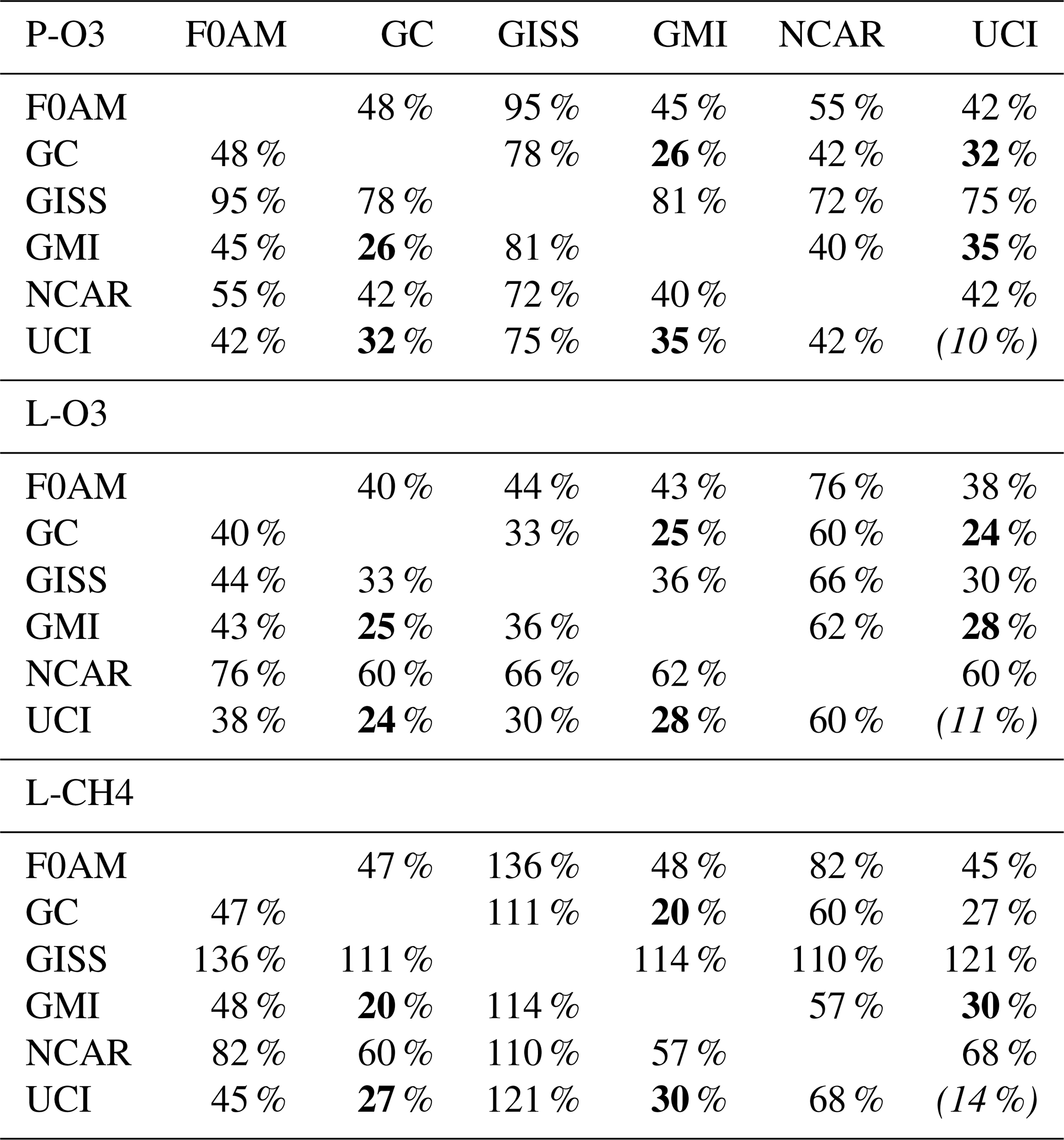
Matrices are symmetric. Calculated with the 31 376 MDS-0 unweighted parcels using the standard RDS protocol. F0AM lacks 5510 of these parcels because there are no reported J values. UCI shows RMSD between years 2016 (default) and 1997 as the value in parentheses on diagonal. The unweighted mean R values from three core models (GC, GMI, UCI) are P-O3 = 1.97, L-O3 = 1.50 and L-CH4 = 0.66; all are in units of ppb/d. The three core-model RMSDs are shown in bold.

4 Results

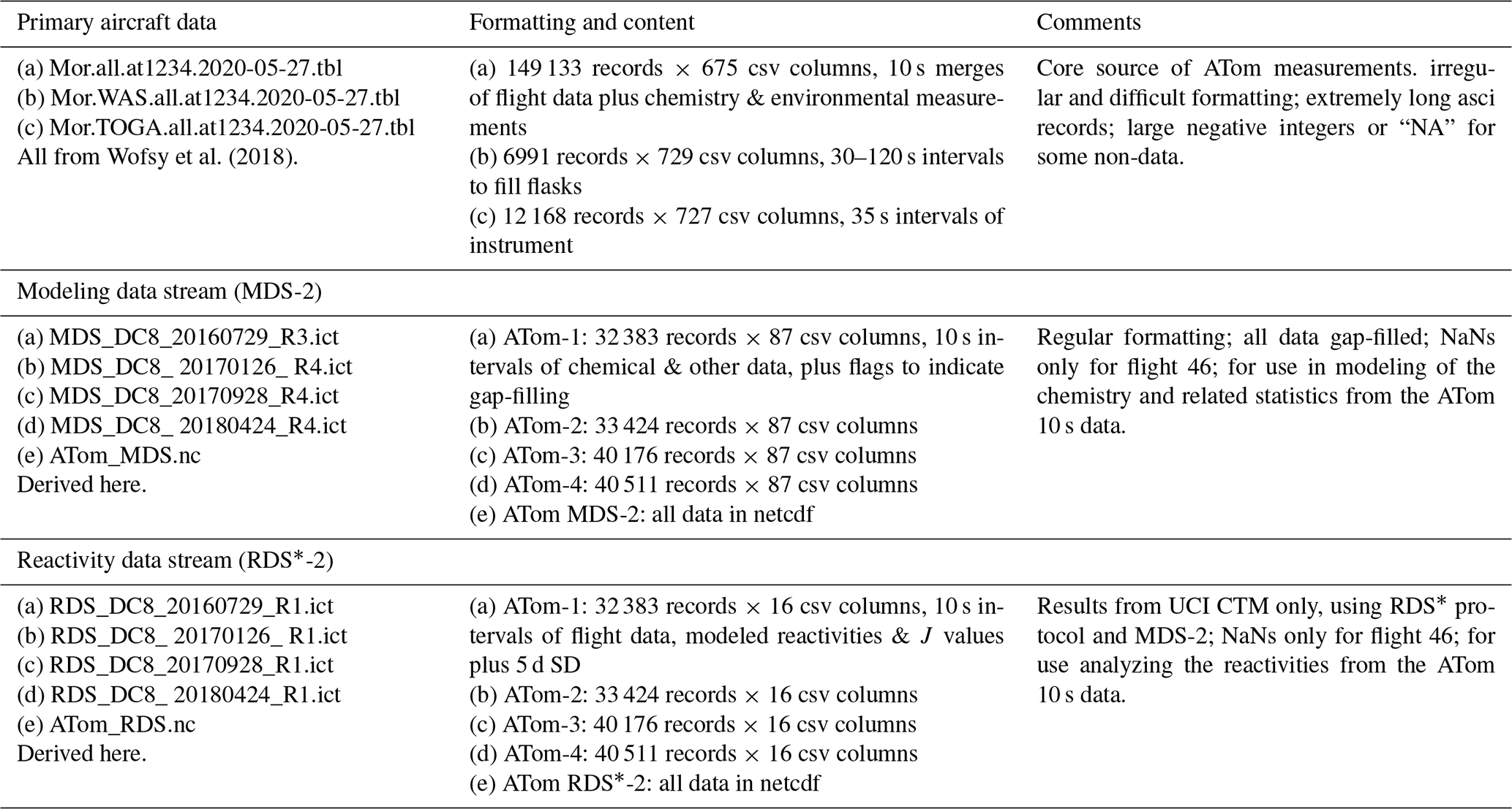
Our analysis of the reactivities uses the six-model RDS-0 results to examine the consistency in calculating the Rs across models. Thereafter, we rely on the similar results from the three central models (GC, GMI, UCI) to justify use of UCI RDS^*-2 as our best estimate for ATom reactivities. The uncertainty in this estimate can be approximated by the inter-model spread of the central models as discussed above. When evaluating the model's climatology for chemical species, we use MDS-2. A summary of the key data files used here, as well as their sources and contents, is given in Table 4.

Table 4 ATom data files used here.

4.1 Probability densities of the reactivities

The reactivities for three large domains (global, Pacific, Atlantic) from the six-model RDS-0 are summarized in Tables 2 and S8. Sorted PDs for the three Rs and Pacific and Atlantic Ocean basins are plotted in Fig. 1 and show the importance of the most reactive “hot” parcels with deeply convex curves and the sharp upturn in R values above 0.9 cumulative weight (top 10 %). Both basins show a similar emphasis on the most reactive hot parcels: 80 %–90 % of total R is in the top 50 % of the parcels, 25 %–35 % is in the top 10 % and about 10 %–14 % is in the top 3 %. The corollary is that the bottom 50 % parcels control only 10 %–20 % of the total reactivity, which is why the median is less than mean (except for P-O3 in the Atlantic). Each R value and each ocean has a unique shape; for example L-O3 in the Atlantic is almost two straight lines breaking at the 50th percentile. In Fig. 1 the agreement across all models (except GISS) is clear, indicating that the conclusion in P2018 (i.e., that most global chemistry models agree on the O₃ and CH₄ budgets if given the chemical composition) also holds for the ATom-measured chemical composition. Comparing the dashed brown (UCI, RDS-0) and black (UCIP, RDS^*-2) lines, we find that the shift to observed NO_x and new HNO₄+PAN protocol has introduced noticeable changes only for P-O3: increasing reactivities overall in the Pacific while decreasing them slightly in the Atlantic. From Table 2, these changes primarily affected mean P-O3 and were due primarily to the shift from MDS-0 to MDS-2 and secondarily to the RDS^* protocol, which reduced both P-O3 and L-O3 in both basins. We conclude that accurate modeling of chemical composition of the 80th and greater percentiles is important but that modest errors in the lowest 50th percentile are inconsequential; effectively, some parcels matter more than others (P2017).

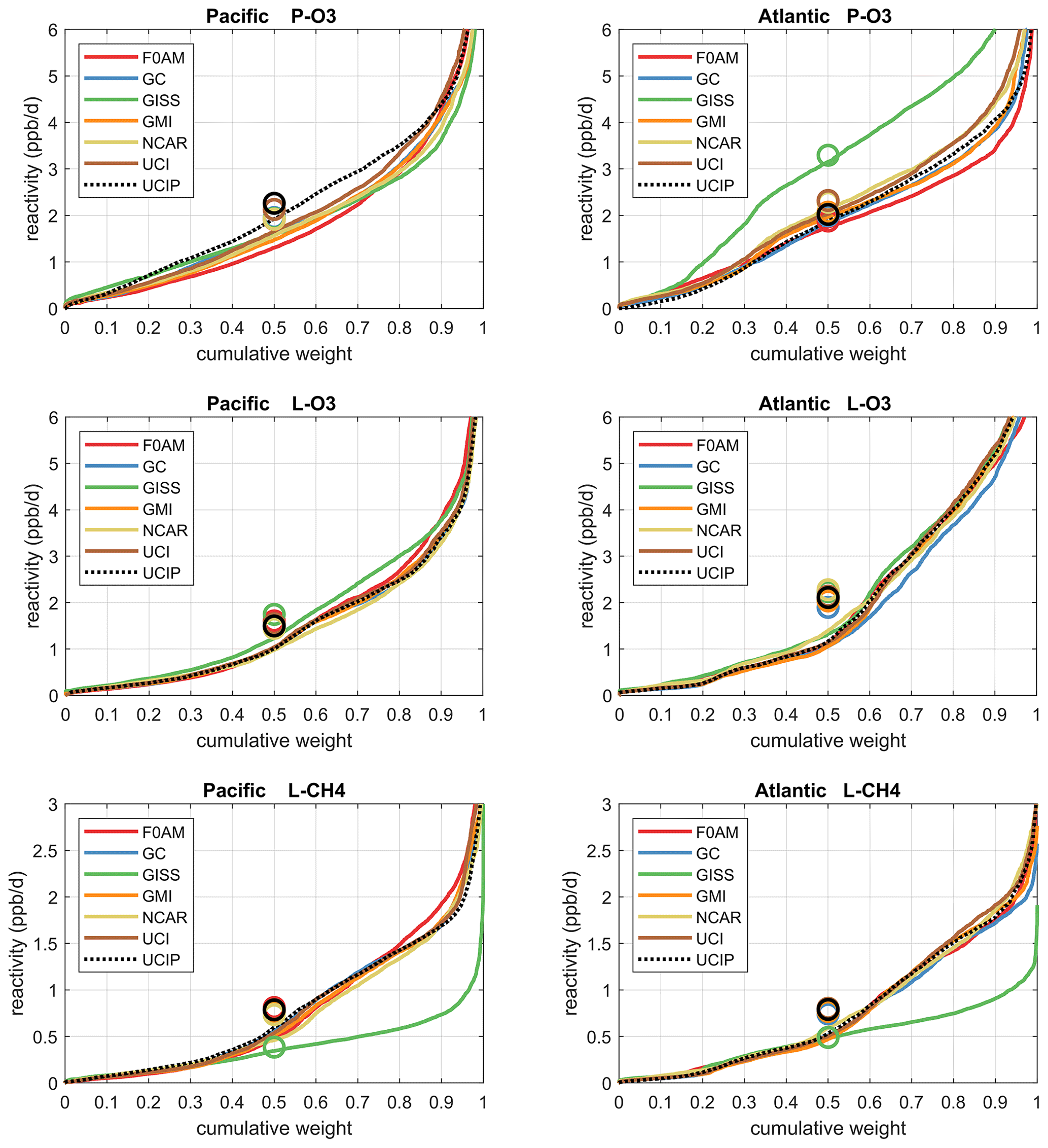
Figure 1 Sorted reactivities (P-O3, L-O3, L-CH4, ppb/d) for the Pacific and Atlantic domains of ATom-1. Each parcel is weighted; see text. The six modeled reactivities for MDS-0 using the standard RDS protocol are shown with colored lines, and the UCI calculation for MDS-2 using the new RDS^* protocol (HNO₄ and PAN damping, denoted UCIP) is shown as a dashed black line. The mean value for each model is shown with an open circle plotted at the 50th percentile. (Flipped about the axes, this is a cumulative probability density function.)

How well does this ATom analysis work as a model intercomparison project? Overall, we find that most models give similar results when presented with the ATom-1 MDS. The broad agreement of the cumulative reactive PDs across a range of model formulations using differing levels of chemical complexity shows this approach is robust. The different protocols for calculating reactivities as well as the uncertainty in cloud fields appear to have a small impact on the shape of the cumulative PDs but are informative regarding the minimum structural uncertainty in estimating the 24 h reactivity of a well-measured air parcel.

4.2 Spatial heterogeneity of tropospheric chemistry

A critical unknown for tropospheric chemistry modeling is what resolution is needed to correctly calculate the budgets of key gases. A similar question was addressed in Yu et al. (2016) for the isoprene oxidation pathways using a model with variable resolution (500, 250 and 30 km) compared to aircraft measurements; see also ship plume chemistry in Charlton-Perez et al. (2009). ATom's 10 s air parcels measure 2 km (horizontal) by 80 m (vertical) during most profiles. There are obviously some chemical structures below the 10 s air parcels we use here. Only some ATom measurements are archived at 1 Hz, and we examine a test case using 1 s data for O₃ and H₂O for a mid-ocean descent between Anchorage and Kona in Fig. S2a in the Supplement. Some of the 1 s (200 m by 8 m) variability is clearly lost with 10 s averaging, but 10 s averaging preserves most of the variability. Lines in Fig. S2 demark 400 m in altitude, and most of the variability appears to occur on this larger, model-resolved scale. Figure S2b shows the 10 s reactivities during that descent and also indicates that much of the variability occurs at 400 m scales. A more quantitative example using all the tropical ATom reactivities is shown in comparisons with probability densities below (Fig. 5).

How important is it for the models to represent the extremes of reactivity? While the sorted reactivity curves (Fig. 1, Tables 2 and S8) continue to steepen from the 90th to 97th percentile, the slope does not change that much. Thus we can estimate the 99th + percentile contributes < 5 % of the total reactivity. Thus, if our model misses the top 1 % of reactive air parcels (e.g., due to the inability to simulate intensely reactive thin pollution layers), then we miss at most 5 % of the total reactivity. This finding is new and encouraging, and it needs to be verified with the ATom-2, 3 and 4 data.

The spatial structures and variability of reactivity as sampled by the ATom tropic transects (central Pacific, eastern Pacific and Atlantic) are presented as nine panels in Fig. 2. Here, the UCI RDS^*-2 reactivities are averaged and plotted in 1^∘ latitude by 200 m thick cells, comparable to some global models (e.g., GMI, NCAR, UCI). We separate the eastern Pacific (121^∘ W, research flight (RF) 1) from the central Pacific (RFs 3, 4 and 5) because we are looking for contiguous latitude-by-pressure structures.

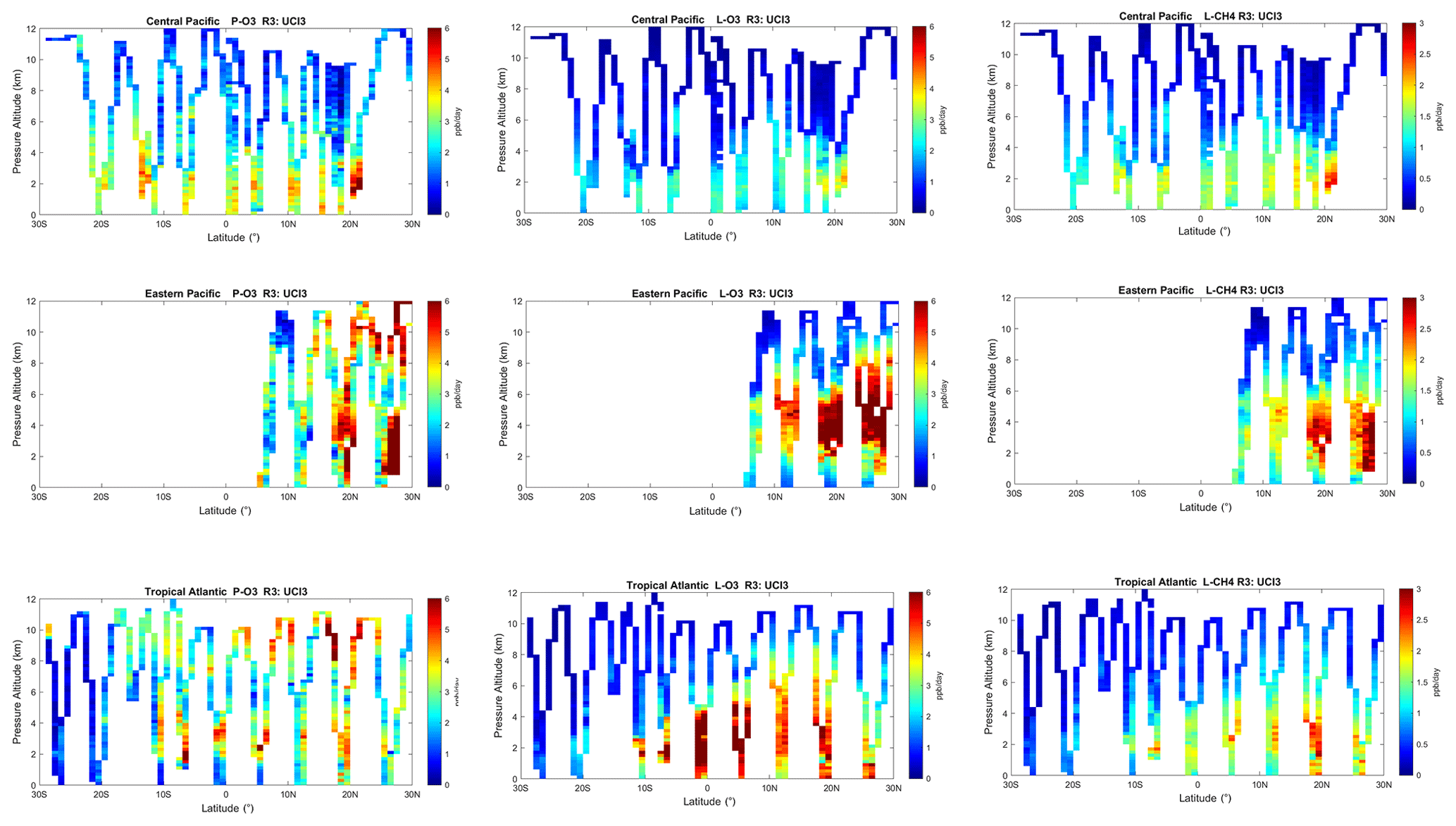
Figure 2 Curtain plots for P-O3 (0–6 ppb/d), L-O3 (0–6 ppb/d) and L-CH4 (0–3 ppb/d) showing the profiling of ATom-1 flights in the central Pacific (RF 3, 4 and 5), eastern Pacific (RF 1) and Atlantic (RF 7, 8 and 9). Reactivities are calculated with the UCI model using MDS-2 and the new RDS^* protocol (UCI RDS^*-2). The 10 s air parcels are averaged into 1^∘ latitude and 200 m altitude bins.

In the central Pacific (row 1), highly reactive (hot) P-O3 parcels (> 6 ppb/d) occur in larger, connected air masses at latitudes 20–22^∘ N and pressure altitudes 2–3 km and in more scattered parcels (> 3 ppb/d) below 5 km down to 20^∘ S. High L-O3 and L-CH4 coincide with this 20–22^∘ N air mass and also with some high P-O3 at lower latitudes. This pattern of overlapping extremes in all three Rs is surprising because the models' mid-Pacific climatologies show a separation between regions of high L-O3 (lower-middle troposphere) and high P-O3 (upper troposphere, as seen in P2017's Fig. 3). The obvious explanation is that the models leave most of the lightning-produced NO_x in the upper troposphere. The ATom profiling seems to catch reactive regions in adjacent profiles separate by a few hundred kilometers, scales easily resolvable with 3D models.

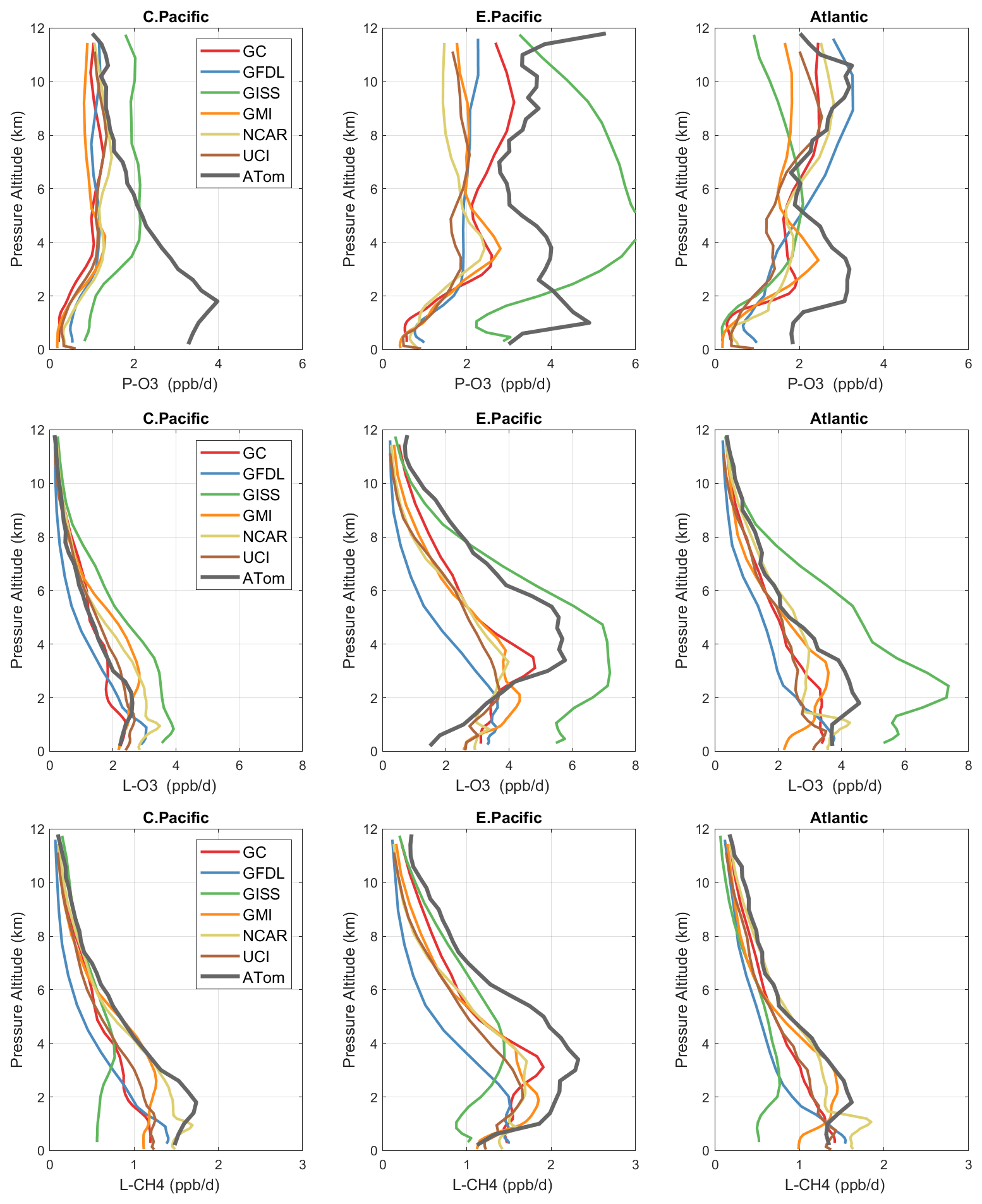
Figure 3 Mean profiles of reactivity (rows: P-O3, L-O3, L-CH4 in ppb/d) in three domains (columns: C. Pacific, 30^∘ S–30^∘ N by 180–210^∘ E; E. Pacific, 0–30^∘ N by 230–250^∘ E; Atlantic, 30^∘ S–30^∘ N by 326–343^∘ E). Air parcels are cosine(latitude)-weighted. ATom-1 (gray) results are from Fig. 2, while model results are taken from the August climatologies in Prather et al. (2017).

In the eastern Pacific (row 2), the overlap of outbound and return profiles enhances the spatial sampling over the 10 h flight. The region of very large L-O3 (> 5 ppb/d) is extensive, beginning at 5–6 km at 10^∘ N and broadening to 2–8 km at 28^∘ N. The region of L-CH4 is similar, but loss at the upper altitudes of this air mass is attenuated because of the temperature dependence of L-CH4 and possibly because of differing OH:HO₂ ratios with altitude. Large P-O3 (> 6 ppb/d) occurs in some but not all of these highly reactive L-O3 regions, suggesting that NO_x is not as evenly distributed as HO_x is. P-O3 also show regions of high reactivity above 8 km that are not in the high L-O3 and L-CH4 regions, probably evidence of convective sources of HO_x and NO_x but too cold and dry for the L-O3 and L-CH4 reactions. ATom-1 RF1 (29 July 2016) occurred during the North American Monsoon when there was easterly flow off Mexico; thus the high reactivity of this large air mass indicates that continental deep convection is a source of high reactivity for both O₃ and CH₄.

In the Atlantic (row 3), we also see similar air masses through successive profiles, particularly in the northern tropics. The Atlantic P-O3 shows high-altitude reactivity similar to the eastern Pacific. Likewise, the large values of L-O3 and L-CH4 match the eastern Pacific and not central Pacific. Unlike either Pacific transect, the Atlantic L-O3 and L-CH4 show some high reactivity below 1 km altitude. Overall, the ATom-1 profiling clearly identifies extended air masses of high L-O3 and L-CH4 extending over 2–5 km in altitude and 10^∘ of latitude. The high P-O3 regions tend to be much more heterogeneous with greatly reduced spatial extent, likely of recent convective origin as for the eastern Pacific.

Overall, the extensive ATom profiling identifies a heterogeneous mix of chemical composition in the tropical Atlantic and Pacific, with a large range of reactivities. What is important for those trying to model tropospheric chemistry is that the spatial scales of variability seen in Fig. 2 are within the capability of modern global models.

4.3 Testing model climatologies

The ATom data set provides a unique opportunity to test CTMs and CCMs in a climatological sense. In this section, we compare ATom-1 data and the six models' chemical statistics for mid-August used in P2017. The ATom profiles cannot be easily compared point by point with CCMs, and we use statistical measures of the three reactivities in the three tropical basins: mean profiles in Fig. 3 and PDs in Fig. 5.

4.3.1 Profiles

For P-O3 profiles (top row, Fig. 3), the discrepancy between models and measurements is stark. The models (less GISS) present a consistent picture of one world, while the ATom profiles describe an entirely different world. In the central Pacific at 8–12 km, the ATom-1 results tend to agree with models, showing ozone production of about 1 ppb/d. Below 8 km, ATom's P-O3 increases to a peak of 4 ppb/d at 2 km, while the models' P-O3 stays constant down to 4 km and then decrease to about 0.5 ppb/d below 2 km. This pattern indicates that in the middle of the Pacific, the NO_x + HO_x combination that produces ozone is suppressed throughout the lower troposphere in all the models. In the eastern Pacific and Atlantic, both models' and ATom reactivities indicate that P-O3 is greatly enhanced above 6 km as compared to the central Pacific, but below 6 km ATom P-O3 is much larger than that of the models', by a factor of 2. In the upper troposphere, the agreement indicates that both models and ATom find the influence of deep continental convection bringing reactive NO_x + HO_x air masses to the nearby oceanic regions but not to the central Pacific. The difference below 5 km in all three regions implies a consistent bias across the models in some combination of HO_x sources and/or the vertical redistribution of lightning NO_x. This difference is unlikely to be a sampling bias in ATom-1, given it occurs in all three regions.

For L-O3 (middle row), the agreement in the central Pacific is very good throughout the 0–12 km range; i.e., ATom looks just like one of the models (except GISS). Moving to the eastern Pacific and Atlantic, both models and ATom show increased reactivity, consistent with continental convective outflow. The large ATom reactivity in the eastern Pacific (3–8 km) is clear in Fig. 2 and likely due to easterly mid-tropospheric flow from convection over Mexico at that specific time (29 July 2016). Similarly, the ATom reactivity at a low level (1–3 km) in the Atlantic is associated with biomass burning in Africa and was measured in other trace species. Thus, in terms of L-O3, the ATom–model differences may be due to specific meteorological conditions, and this could be tested with CTMs using 2016 meteorology and wildfires.

For L-CH4 (bottom row), the ATom–model pattern is similar to L-O3, but higher ATom reactivity occurs at lower altitudes. Overall, the ATom L-CH4 is slightly greater than the modeled L-CH4. L-O3 is dominated by O(1D) and HO₂ loss, while L-CH4 is limited to OH loss. Overall, there is clear evidence that the Atlantic and Pacific have very different chemical mixtures controlling the reactivities and that convection over land (monsoon or biomass burning) creates air masses that are still highly reactive a day or so later.

4.3.2 Key species

The deficit in modeled P-O3 points to a NO_x deficiency in the models, and this becomes obvious in the comparison of the PD histograms for NO_x shown in Fig. 4. In the central Pacific over 0–12 km (first row), ATom has a reduced frequency of parcels with 2–20 ppt and corresponding increase in parcels with 20–80 ppt. This discrepancy is amplified in the lower troposphere, 0–4 km (second row). In the middle of the Pacific, our chemistry models are missing a large source of lower tropospheric NO_x. The obvious source of oceanic NO_x is lightning since oceanic sources of organonitrates or other nitrate species measured on ATom could not supply this amount. The ATom statistics indicate a lightning source must be vertically mixed. In the eastern Pacific, the ATom 0–4 km troposphere appears again to have large amounts of air with 20–50 ppt, while the full troposphere more closely matches the models, except for the large occurrence of air with 100–300 ppt NO_x. These high-NO_x upper troposphere regions are probably direct outflow from very deep convection with lightning in the monsoon regions over Mexico at this time. In the Atlantic, the models' NO_x shows too frequent occurrence of low NO_x (< 10 ppt) and thus underestimates the 10–100 ppt levels at all altitudes. ATom has a strong peak occurrence about 80–120 ppt in the upper troposphere, and, like the eastern Pacific, this is probably due to lightning NO_x from deep convection over land (Africa or South America). Overall, the models appear to be missing significant NO_x sources throughout the tropics, especially below 4 km.

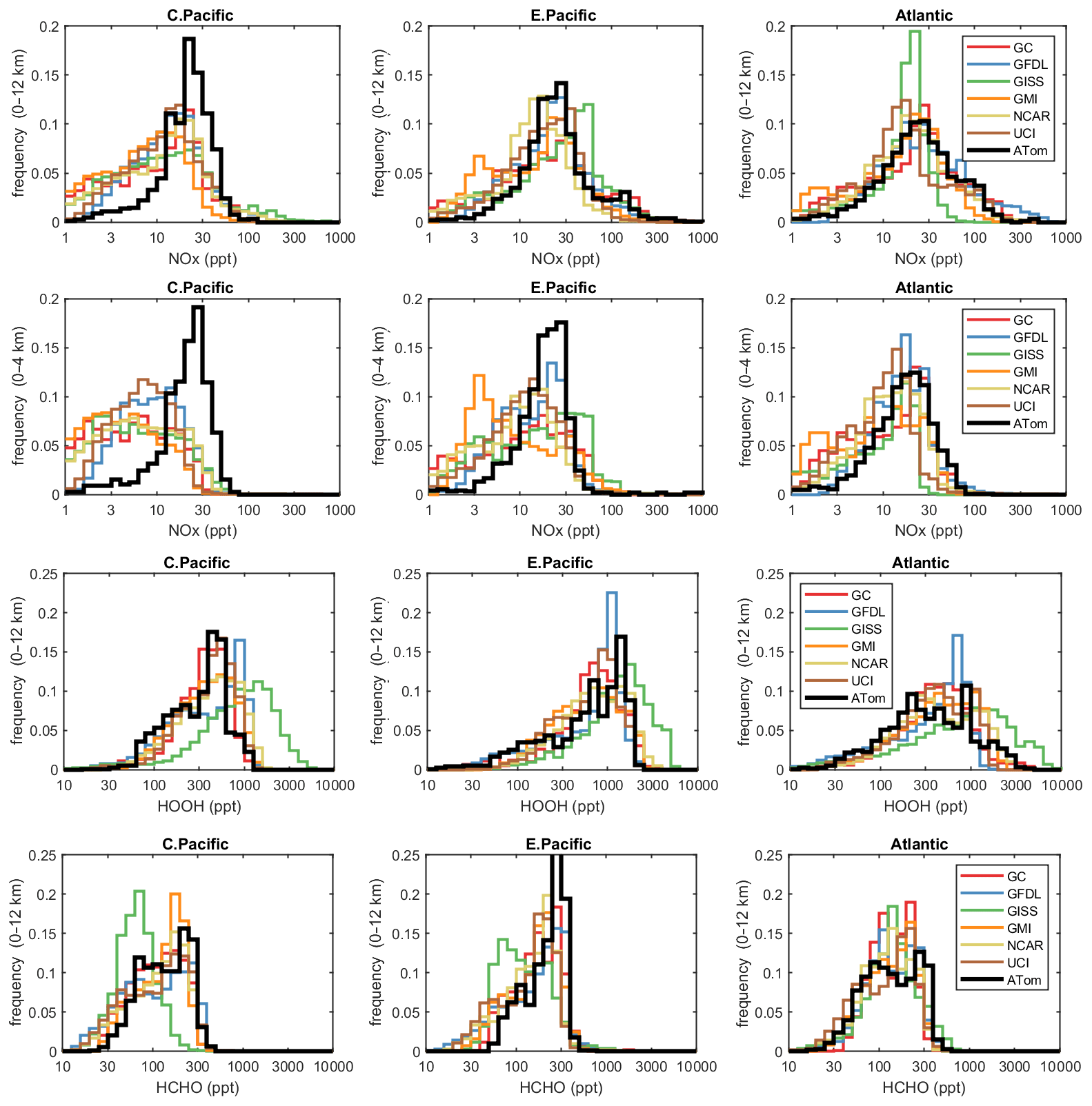
Figure 4 Histograms of probability densities (PDs) of NO_x (0–12 km, row 1), NO_x (0–4 km, row 2), HOOH (0–12 km, row 3) and HCHO (0–12 km, row 4) for the three tropical regions (central Pacific, eastern Pacific, Atlantic). The ATom-1 data are plotted on top of the six global chemistry models' results for a day in mid-August and sampled as described in Fig. 3.

In Fig. 4, we also look at the histograms for the key HO_x-related species HOOH (third row) and HCHO (fourth row). For these species, the ATom–model agreement is generally good. If anything, the models tend to have too much HOOH. ATom shows systematically large occurrences of low HOOH (50–200 ppt, especially central Pacific), indicating, perhaps, that convective or cloud scavenging of HOOH is more effective than is modeled. HCHO shows reasonable agreement in the Atlantic, but in both central and eastern Pacific, the modeled low end (< 40 ppt) is simply not seen in the ATom data. Also, the models are missing a strong HCHO peak at 300 ppt in the eastern Pacific, probably convection-related. Thus, in terms of these HO_x precursors, the model climatologies appear to be at least as reactive as the ATom data.

While the ATom-1 data in Fig. 4 are limited to single transects, the model NO_x discrepancies apply across the three tropical regions, and the simple chemical statistics for these flights alone are probably enough to identify measurement-model discrepancies. For the HO_x-related species, the models match the first-order statistics from ATom. In terms of using ATom statistics as a model metric, it is encouraging that where individual models tend to deviate from their peers, they also deviate from the ATom-1 PDs.

4.3.3 Probability densities

Mean profiles do not reflect the heterogeneity seen in Fig. 2, and so we also examine the PDs of the tropical reactivities (Fig. 5). The model PDs (colored lines connecting open circles at the center of each bin) are calculated from the 1 d statistics for mid-August (P2017) using the model blocks shown in Fig. S1. The model grid cells are weighted by air mass and cosine(latitude) and limited to pressures greater than 200 HPa. The ATom PDs (black lines connecting black open circles) are calculated from the 10 s data weighted by (but not averaged over) the number of points in each 10^∘ latitude by 200 hPa pressure bin and then also by cosine (latitude) to compare with the models. In addition, a PD was calculated from the 1^∘ by 200 m average grid-cell values in Fig. 2 (black Xs), and this is also cosine(latitude)-weighted. To check if the high reactivities in the eastern Pacific affected the whole Pacific PD, a separate PD using only central Pacific 10 s data was calculated (gray lines connecting gray open circles). The mean reactivities (ppb/d) from the models and ATom are given in the legend; note that these values disagree with some table data that are not cosine-weighted. The PD binning is shown by the open circles, and occurrences of off-scale reactivities are included in the last point.

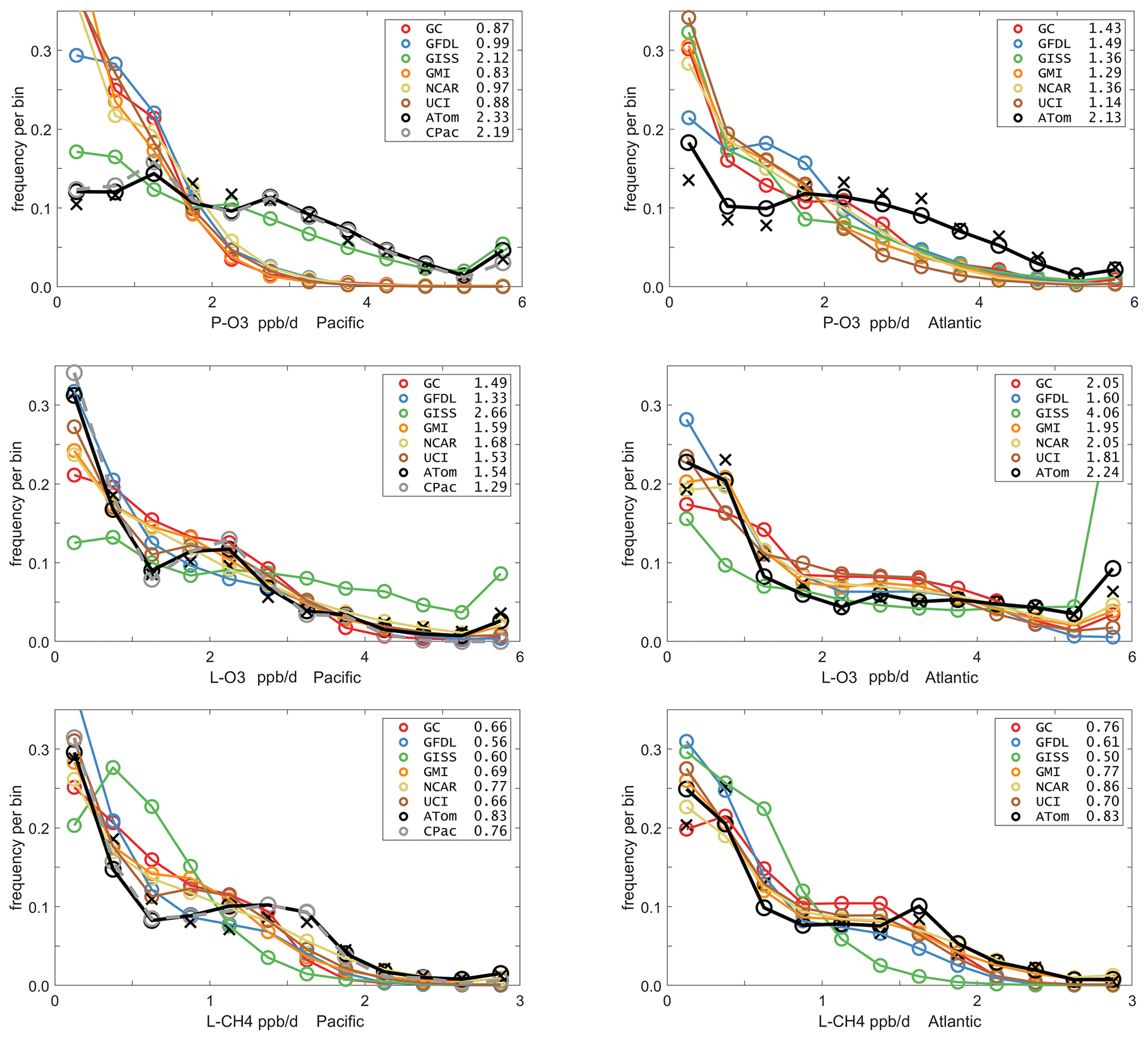
Figure 5 Probability densities (PDs, frequency of occurrence) for the ATom-1 three reactivities (rows: P-O3, L-O3, L-CH4 in ppb/d) and for the Pacific and Atlantic from 54^∘ S to 60^∘ N (columns left and right). Each air parcel is weighted as described in the text for equal frequency in large latitude–pressure bins and also by cosine(latitude). The ATom statistics are from the UCI model, using MDS-2 and revised RDS^* protocol (HNO₄ and PAN damping). The full Pacific results (solid black) also show just the central Pacific (dashed gray). The six models' values for a day in mid-August are averaged over longitude for the domains shown in Fig. S1 and then cosine(latitude)-weighted. Mean values (ppb/d) are shown in the legend but are different from some tables where the cosine weighting is not applied. The PD derived from the ATom 10 s parcels binned at 1^∘ latitude and 200 m altitude (shown for the tropics only in Fig. 2) is typical of a high-resolution global model and denoted by black Xs.

The obvious discrepancy is with P-O3 in both Pacific and Atlantic basins. ATom data have very low occurrence of P-O3 < 1 ppb/d and a broad, almost uniform frequency (∼ 0.1) extending out to 4 ppb/d. This result is consistent with the mean profile errors (Fig. 3). The match for L-CH4 is very good in both basins, although the models have a greater occurrence in the middle 0.5–1.5 ppb/d range and reduced occurrence in the higher 1.5–2.5 ppb/d range. For L-O3, the match is very good and similar to L-CH4, although the Atlantic has a high frequency of L-O3 > 6 ppb/d that is not seen in the models (except GISS). The extreme eastern Pacific reactivities are seen in the mean values displayed in the legend (e.g., CPac with 1.29 ppb/d L-O3 versus ATom (i.e., CPac + EPac) with 1.54 ppb/d), but the PDs (gray circles versus black circles) resemble each other more closely than any of the models.

The ability to test a model's reactivity statistics with the ATom 10 s data is not obvious, but the PDs based on 1^∘ latitude by 200 m altitude cells (the black Xs) is remarkably close to the PDs based on 2 km (horizontal) by 80 m (vertical) 10 s parcels. With the coarser resolution, we see a slight shift of points from the ends of the PD to the middle as expected, but we find once again, that the loss in high-frequency, below-model grid-cell resolution is not great. Both ATom-derived PDs more closely resemble each other than any model PD. Thus, current global chemistry models with resolutions of about 100 km by 400 m should be able to capture much of the wide range of chemical heterogeneity in the atmosphere, which for the oceanic transects is, we believe, adequately resolved by the 10 s ATom measurements. Perhaps more surprising, given the different mean profiles in Fig. 3, is that the five model PDs in Fig. 5 look very much alike. This points to some significant underlying difference between our current global chemistry models and the ATom observations.

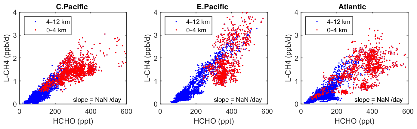
Figure 6 Scatterplot of L-CH4 (ppb/d) versus HCHO (ppt) for ATom 1 in the three tropical regions shown in Fig. 3. The air parcels are split into the lower troposphere (0–4 km pressure altitude, red dots), where most of the reactivity lies, and the middle and upper troposphere (4–12 km, blue). A simple linear fit to all data is shown (thin black line), and the slope is given in units of 1 per day.

5 Discussion and path forward

5.1 Major findings

This paper opens a door for what the community can do with the ATom measurements and the derived products. ATom's mix of key species allows us to calculate the reactivity of the air parcels and hopefully may become standard for tropospheric chemistry campaigns. We find that the reactivity of the troposphere with respect to O₃ and CH₄ is dominated by a fraction of the air parcels but not by so small and infrequent a fraction as to challenge the ability of current CTMs to simulate these observations and thus be used to study the oxidation budgets. In comparing ATom results with modeled climatologies, we find a clear model error – missing O₃ production over the tropical oceans' lower troposphere – and traced it to the lack of NO_x below 4 km. The occurrence of the same error over the central and eastern Pacific as well as the Atlantic Ocean makes this a robust model–measurement discrepancy.

Building our chemical statistics (PDs) from the ATom 10 s air parcels on a scale of 2 km by 80 m, we can identify the fundamental scales of spatial heterogeneity in tropospheric chemistry. Although heterogeneity occurs at the finest scales (such as seen in some 1 s observations), the majority of variability in terms of the O₃ and CH₄ budgets occurs across scales larger than neighboring 2 km parcels. The PDs measured in ATom can be largely captured by global models' 100 km by 200 m grid cells in the lower troposphere. This surprising result is evident by comparing the ATom 1D PDs – both species and reactivities – with those from the models' climatologies (Fig. 5). These comparisons show that the modeled PDs are consistent with the innate chemical heterogeneity of the troposphere as measured by the 10 s parcels in ATom. A related conclusion for biomass burning smoke particles is found by Schill et al. (2020), where most of the smoke appears in the background rather than in pollution plumes, and therefore much of the variability occurs on synoptic scales resolved by global models (see their Fig. 1 compared with Fig. 2 here).

Figure 7 2D frequency of occurrence (PDs in log ppt mole fraction) of HOOH vs. NO_x for the tropical central Pacific for all four ATom deployments. The cross marks the mean (in log space), and the ellipse is fitted to the rotated PD having the smallest semi-minor axis. The semi-minor and semi-major axes are 2 standard deviations of PD in that direction. The ellipses from ATom-2 (red), ATom-3 (blue) and ATom-4 (dark green) are also plotted in the ATom-1 quadrant.

5.2 Opportunities and lessons learned

As a quick look at the opportunities provided by the ATom data, we present an example based on the Wolfe et al. (2019) study, which used the F0AM model and semi-analytical arguments to show that troposphere HCHO columns (measurable by satellite and ATom) are related to OH columns (measured by ATom) and thus to CH₄ loss. Figure 6 extends the Wolfe et al. study using the individual air parcels and plotting L-CH4 (ppb/d) versus HCHO (ppt) for the three tropical regions where most of the CH₄ loss occurs. The relationship is linear, with slopes ranging from 4 to 6 per day, but the largest reactivities (0–4 km, 1–3 ppb/d) are not so well correlated with HCHO.

As is usual with new model intercomparison projects, we have an opportunity to identify model “features” and identify errors. In the UCI model, an error in the lumped alkane formulation (averaging alkanes C₃H₈ and higher) did not show up in P2018, where UCI supplied all the species, but when the ATom data were used, the UCI model became an outlier. Once found, this problem was readily fixed. The divergence of the NCAR RDS results is likely due to the implementation of the RDS protocol where CCM values overwrite the MDS values. We identified this problem in P2018 and thought it was solved, but perhaps it is not. Inclusion of the F0AM model with its extensive hydrocarbon oxidation mechanism provided an interesting contrast with the simpler chemistry in the global CCM/CTMs. For a better comparison of the chemical mechanisms, we should have F0AM use 5 d of photolysis fields from one of the CTMs. The anomalous GISS results have been examined by a co-author, but no clear causes have been identified as of this publication. The problem goes beyond just the implementation of the RDS protocol, as it shows up in the model climatology (Figs. 4 and 5, also in P2017).

Decadal-scale shifts in the budgets of O₃ and CH₄ are likely to be evident through the statistical patterns of the key species, rather than simply via average profiles. The underlying design of ATom was to collect enough data to develop such a multivariate chemical climatology. As a quick look across the four deployments, we show the joint 2D PDs on a logarithmic scale as in P2017 for HOOH versus NO_x in Fig. 7. The patterns for the tropical central Pacific are quite similar for the four seasons of ATom deployments, and the fitted ellipses are almost identical for ATom 2, 3 and 4. Thus, for these species in the central Pacific, we believe that ATom provides a benchmark of the 2016–2018 chemical state, one that can be revisited with an aircraft mission in a decade to detect changes in not only chemical composition, but also reactivity.

ATom identifies which “highly reactive” spatial or chemical environments could be targeted in future campaigns for process studies or to provide a better link between satellite observations and photochemical reactivity (e.g., E. Pacific mid-troposphere in August, Fig. 2). The many corollary species measured by ATom (not directly involved in CH₄ and O₃ chemistry) can provide clues to the origin or chemical processing of these environments. We hope to engage a wider modeling community beyond the ATom science team, as in H2018, in the calculation of photochemical processes, budgets, and feedbacks based on all four ATom deployments.