In situ ozone production is highly sensitive to volatile organic compounds in Delhi, India

The Indian megacity of Delhi suffers from some of the poorest air quality in the world. While ambient NO₂ and particulate matter (PM) concentrations have received considerable attention in the city, high ground-level ozone (O₃) concentrations are an often overlooked component of pollution. O₃ can lead to significant ecosystem damage and agricultural crop losses, and adversely affect human health. During October 2018, concentrations of speciated non-methane hydrocarbon volatile organic compounds (C₂–C₁₃), oxygenated volatile organic compounds (o-VOCs), NO, NO₂, HONO, CO, SO₂, O₃, and photolysis rates, were continuously measured at an urban site in Old Delhi. These observations were used to constrain a detailed chemical box model utilising the Master Chemical Mechanism v3.3.1. VOCs and NO_x (NO + NO₂) were varied in the model to test their impact on local O₃ production rates, P(O₃), which revealed a VOC-limited chemical regime. When only NO_x concentrations were reduced, a significant increase in P(O₃) was observed; thus, VOC co-reduction approaches must also be considered in pollution abatement strategies. Of the VOCs examined in this work, mean morning P(O₃) rates were most sensitive to monoaromatic compounds, followed by monoterpenes and alkenes, where halving their concentrations in the model led to a 15.6 %, 13.1 %, and 12.9 % reduction in P(O₃), respectively. P(O₃) was not sensitive to direct changes in aerosol surface area but was very sensitive to changes in photolysis rates, which may be influenced by future changes in PM concentrations. VOC and NO_x concentrations were divided into emission source sectors, as described by the Emissions Database for Global Atmospheric Research (EDGAR) v5.0 Global Air Pollutant Emissions and EDGAR v4.3.2_VOC_spec inventories, allowing for the impact of individual emission sources on P(O₃) to be investigated. Reducing road transport emissions only, a common strategy in air pollution abatement strategies worldwide, was found to increase P(O₃), even when the source was removed in its entirety. Effective reduction in P(O₃) was achieved by reducing road transport along with emissions from combustion for manufacturing and process emissions. Modelled P(O₃) reduced by ∼ 20 ppb h⁻¹ when these combined sources were halved. This study highlights the importance of reducing VOCs in parallel with NO_x and PM in future pollution abatement strategies in Delhi.

1 Introduction

The majority of the world's population now lives in urban areas. This is projected to increase from 55 % in 2018 to 68 % of the global population by 2030, with 90 % of this growth occurring in Asia and Africa (Molina, 2021; United Nations, Department of Economic and Social Affairs, Population Division, 2019, 2018). Rapidly increasing industrialisation and urbanisation, coinciding with fast population growth, have led to worsening air quality in many of these densely populated regions. This is driven by the increasing emissions of nitrogen oxides (NO_x = NO + NO₂), largely associated with transport, and volatile organic compounds (VOCs), released from a diverse range of sources. Photochemical reactions in the atmosphere then lead to the formation of a wide range of important secondary pollutants, including ozone (O₃) and secondary inorganic and organic aerosol.

Tropospheric O₃ is both an air pollutant and an important greenhouse gas throughout the troposphere (Skeie et al., 2020). High levels of O₃ can adversely affect vegetation, global crop yields (Avnery et al., 2011), and human health, with long-term exposure increasing the risk of death from cardiovascular and respiratory illnesses (Jerrett et al., 2009), and short-term exposure leading to the exacerbation of asthma in children (Thurston et al., 1997). O₃ exposure has been linked to both acute and chronic pulmonary and cardiovascular health outcomes through both animal toxicological and human clinical studies, with one study showing statistically significant decreases in the lung function of adults on an average exposure of 70 ppbV of O₃ across five 6.6 h windows (WHO, 2005, 2013; Schelegle et al., 2009; EPA, 2020; Fleming et al., 2018).

As a result of increased anthropogenic emissions, tropospheric O₃ increased globally during the 20th century and has continued to rise regionally in Asia during the 21st century (Fleming et al., 2018; Royal Society, 2008; Lu et al., 2020). Background tropospheric O₃ has also continued to increase (Parrish et al., 2014; Tarasick et al., 2019). Since the 1990s, surface O₃ trends have varied by region (Gaudel et al., 2018; Cooper et al., 2020; Lu et al., 2020), but trends in the free troposphere have been overwhelmingly positive (Gaudel et al., 2020; Liao et al., 2021). Both satellite data and global chemical transport models have identified India and East Asia as the region with the greatest O₃ increases between 1980–2016 (Ziemke et al., 2019), with the rate of change per decade between 2005–2016 more than double that of the rate between 1979–2005 (Ziemke et al., 2019).

Unlike other pollutants such as NO_x and SO₂, ground-level O₃ is not directly emitted but is formed in the atmosphere from the photochemical processing of a range of reactive precursor species (Calvert et al., 2015). O₃ reduction strategies are complicated by its non-linear relationship with its precursor species (NO_x, CO, and VOCs); their reduction does not necessarily lead to a reduction in O₃, and O₃ production is also influenced by longer-lived gases such as CH₄ and CO. The urban atmosphere can be classified as being either VOC-limited or NO_x-limited. In a VOC-limited environment, O₃ can be effectively reduced by reducing VOCs, whereas decreasing NO_x may have a limited effect or even increase the local O₃ production rate, P(O₃) (Li et al., 2021). In a NO_x-limited regime, reducing NO_x emissions is the most efficient approach for reducing P(O₃). Before implementing emission abatement strategies, it is therefore important to consider which regime prevails. Highly populated urban areas are commonly VOC-limited, meaning reducing NO_x without also reducing VOC sources may potentially lead to an increase in local P(O₃) (Sillman, 1999; Sillman et al., 1990) and hence to an increase in ground-level O₃ concentrations.

In general, O₃ formation is mediated by the reactions of peroxy radicals, RO₂ and HO₂, formed in the OH-initiated oxidation of VOCs (Reaction R1), with NO to produce NO₂ (Reactions R2 and R4). NO₂ is then rapidly photolysed back to NO, forming O(³P) (Reaction R5), which can rapidly react with O₂, leading to O₃ (Reaction R6). This recycling of NO to NO₂ leads to net production of O₃ (Calvert et al., 2015). A description of how net O₃ production, P(O₃), is calculated from observed and modelled concentrations can be found in Sect. 3.4.

$$\begin{array}{}\text{(R1)}& {\displaystyle }\mathrm{RH}+\mathrm{OH}+{\mathrm{O}}_{\mathrm{2}}\to {\mathrm{RO}}_{\mathrm{2}}+{\mathrm{H}}_{\mathrm{2}}\mathrm{O}\text{(R2)}& {\displaystyle }{\mathrm{RO}}_{\mathrm{2}}+\mathrm{NO}\to \mathrm{RO}+{\mathrm{NO}}_{\mathrm{2}}\text{(R3)}& {\displaystyle }{\mathrm{RO}}_{\mathrm{2}}+{\mathrm{O}}_{\mathrm{2}}\to {\mathrm{R}}^{\prime }=\mathrm{O}+{\mathrm{HO}}_{\mathrm{2}}\text{(R4)}& {\displaystyle }{\mathrm{HO}}_{\mathrm{2}}+\mathrm{NO}\to \mathrm{OH}+{\mathrm{NO}}_{\mathrm{2}}\text{(R5)}& {\displaystyle }{\mathrm{NO}}_{\mathrm{2}}+hv\to \mathrm{NO}+\mathrm{O}{(}^{\mathrm{3}}\mathrm{P})(\mathit{\lambda }<\mathrm{420}\mathrm{nm})\text{(R6)}& {\displaystyle }\mathrm{O}{(}^{\mathrm{3}}\mathrm{P})+{\mathrm{O}}_{\mathrm{2}}(+M)\to {\mathrm{O}}_{\mathrm{3}}(+M)\end{array}$$

The propensity of a particular VOC species to enhance O₃ production is determined by its reactivity, structure, and ambient concentration (Jenkin et al., 2017). The sources of emissions, and their relative magnitudes, differ between cities, leading to differences in the role played by individual VOCs with respect to O₃ production. Previous studies in megacities have found that a range of different VOC classes lead to ground-level O₃ production. A comprehensive study of chemical processing in London, during the 2012 summer ClearfLo campaign, found biogenic and longer-chain VOCs from diesel sources to be of greatest importance to VOC–hydroxyl radical reactivity and thus in situ O₃ formation (Dunmore et al., 2015; Whalley et al., 2016). Studies investigating the sensitivity of O₃ production to different VOC classes in Shanghai (2006–2007) found that monoaromatic species dominated, accounting for 45 % of the total O₃ production (Geng et al., 2008). Another study in Shanghai (summer 2009) identified significant contributions to O₃ production from but-2-enes (Ran et al., 2011). Biogenic species, such as isoprene, were found to have the greatest impact on OH reactivity, k(OH), an indicator for O₃ production, in Seoul in 2015 (Kim et al., 2016) and the Pearl River Delta in 2006 (Lou et al., 2010), whereas another study pointed to the importance of monoaromatics, followed by isoprene and anthropogenic alkenes to O₃ production in Seoul in spring 2016 (Simpson et al., 2020). These studies incorporated a variety of chemical detail into their models, dependent on the breadth of their VOC measurement suite, with many studies not accounting for oxygenated or biogenic species other than isoprene (Lou et al., 2010). Zavala et al. (2020) show that the key contributors to VOC–OH reactivity in the Mexico City Metropolitan Area (MCMA) between the 1990s and 2019 have changed, with aromatic and alkene contributions decreasing with reduced VOC emissions from mobile source. Oxygenated VOCs from solvent consumption and personal care products dominate the VOC–OH reactivity in recent years, leading to sustained high O₃ concentrations in the MCMA (McDonald et al., 2018; Zavala et al., 2020). Understanding which precursor species are key to O₃ production in any given city allows governments to introduce measures to combat air quality problems (Molina, 2021).

Over the past two decades, advances in vehicle emission technology, along with improvements in residential heating, have led to decreased NO_x emissions in industrialised and highly populated regions of the western world (Georgoulias et al., 2019). In many European cities, additional measures banning vehicle types in busy areas during weekdays, and upgrading the heavy goods vehicle (HGV) fleet, have led to further reductions in ambient NO₂ (Font et al., 2019). In 2013, China introduced the Air Pollution Prevention and Control Action Plan (Zhang et al., 2019). New measures included the improvement of industrial emissions standards, the promotion of cleaner fuels to replace coal in the residential sector, and the removal of older vehicles from the roads. As a result of these new controls, NO₂ emissions in Beijing have decreased by 32 % since 2012 (Krotkov et al., 2016; Liu et al., 2016; Miyazaki et al., 2017). Despite these successes, surface O₃ pollution across China has continued to increase (M. Li et al., 2019; Lu et al., 2018a). The overall O₃ formation potential (OFP) of VOCs has increased alongside this, despite reduction strategies leading to reduced emissions of alkanes and alkenes. This is explained by an increasing emission of VOC species with higher OFPs, such as toluene and xylenes, driven by solvent use and industrial processes (M. Li et al., 2019).

The megacity of Delhi, with an estimated population of over 28 million in 2018 (United Nations, Department of Economic and Social Affairs, Population Division, 2019), suffers from some of the world's poorest air quality (WHO, 2014). Significant efforts have been made over the past two decades to reduce the air pollution burden in Delhi, including the introduction of fuel quality standards, a new metro system to improve public transport, and an odd–even traffic number plate system (Bansal and Bandivadekar, 2013; Kumar et al., 2017). Since the late 1980s, steps to mitigate the impacts of vehicle and fuel emissions in India have been implemented. Initial interventions included switching to compressed natural gas (CNG) for auto rickshaws and buses in Delhi and other major cities. Since 2010, Bharat IV fuel quality standards have been implemented across cities in India, based on the 2003 Auto Fuel Policy. These changes have resulted in reduced annual NO_x emissions nationally, compared with the projected emissions without policy implementation (Bansal and Bandivadekar, 2013).

A recent study of the implications of the SARS-CoV-2 pandemic on air quality compared pollutant levels of PM_2.5, PM₁₀, NO₂, CO, and O₃ in Delhi, and across other Indian cities, before and after a national lockdown (Jain and Sharma, 2020; Mahato et al., 2020; Sharma et al., 2020). The results showed significant improvements in post-lockdown air quality, with reductions in ambient NO_2, PM_2.5, and PM₁₀ exceeding 50 % compared to business as usual. However, increased concentrations of ground-level O₃ (>10 %) were also observed and were attributed to reductions of NO leading to reduced consumption of O₃. Another study found, after removing meteorological biases, concentrations of NO₂ and PM_2.5 at urban background sites in Delhi to have reduced by ∼ 51 % and ∼ 5 % respectively, with O₃ concentrations increasing by ∼ 8 % (Shi et al., 2021). Prior to the SARS-CoV-2 pandemic, studies have observed high concentrations of ambient O₃ in New Delhi, with high levels associated with anti-cyclonic conditions (sunny and warm, stagnant winds and lower humidity) typical during October, the month in which the observational dataset used in this study was obtained (Jain et al., 2005; Sharma et al., 2016). Poor air quality is exacerbated in late October–November, when additional O₃ precursor pollutants are emitted from regional agricultural biomass burning of crop residues within the wider area, and from firecrackers and the burning of effigies as part of seasonal festivities (Jain et al., 2014; Sawlani et al., 2019).

Several recent studies have examined the sources of VOCs in Delhi. Top-down and bottom-up approaches have shown gas-phase organic air pollution to be predominantly from petrol (gasoline) and diesel fuel sources. In two 2018 studies at two different urban sites in Delhi, Stewart et al. (2021a) and Wang et al. (2020) showed that 52 % and 57 % of the measured mixing ratio were from combined petrol and diesel sources. Smaller contributions to the overall VOC burden were found from solid fuel combustion, 16 % (Stewart et al., 2021a) and 27 % (Wang et al., 2020). These data were in line with Guttikunda and Calori (2013), who produced an inventory which showed that petrol and diesel sources were responsible for 65 % by mass of hydrocarbons in Delhi. VOC emissions have also been shown to be dominated by petrol and diesel sources (∼ 50 %) in a study which conducted positive matrix factorisation (PMF) analysis on proton transfer reaction mass spectrometer flux measurements taken in a follow-on campaign in early November 2018 at the Indira Gandhi Delhi Technical University for Women (IGDTUW) (Cash et al., 2021).

There have been several recent studies focused on understanding VOC emissions from sources specific to Delhi. Stewart et al. (2021b) studied the types of intermediate-volatility and semi-volatile gases released from solid fuels in Delhi to better understand their potential impact on air quality, and Stewart et al. (2021c) produced highly speciated non-methane VOC (NMVOC) emission factors from a range of solid fuel combustion sources characteristic to Delhi, which were used by Stewart et al. (2021d) in regional policy models and global chemical transport models. Stewart et al. (2021e) found that fuel wood, crop residue, cow dung cake, and municipal solid waste burning were shown to be 30, 90, 120, and 230 times more reactive with the OH radical, which can lead to O₃ formation, than liquified petroleum gas (LPG), and may be one the factors for the high O₃ levels, and overall poor air quality, observed.

To implement successful ground-level O₃ reduction strategies, a good understanding of the non-linear, chemically complex processing of its precursor species is imperative. This paper presents a comprehensive in situ O₃ production sensitivity study, using an extensive speciated VOC and oxygenated VOC (o-VOC) measurement suite obtained in Delhi during the Atmospheric Pollution and Human Health programme in an Indian Megacity (APHH-India) DelhiFlux project post-monsoon field campaign in October 2018. Measurements of NO_x, CO, SO₂, O₃, HONO, 34 photolysis rates, pressure, temperature, and relative humidity complete the dataset. The observations were used to constrain a detailed zero-dimensional chemical box model, incorporating the Master Chemical Mechanism v3.1.1 (MCM: http://mcm.york.ac.uk, last access: March 2020). Significant VOC classes and sources contributing to the OH reactivity (k(OH)) are identified by constraining the model to the full VOC suite. By modifying the constraints of these species, their contribution to in situ O₃ production was investigated by comparing relative changes in the modelled rate of O₃ production. The sensitivity of in situ O₃ production to changes in NO, photolysis, and particulate matter (PM) was also investigated.

2 Experimental

2.1 Site description

The APHH-India DelhiFlux post-monsoon measurement campaign took place between 4 October and 5 November 2018. The primary measurement site was located on the campus of the IGDTUW, near Kashmere Gate in Old Delhi (28.67^∘ N, 77.23^∘E). The campus is an open area, with some green spaces, and is close to major roads and highways: 1.5 km north of the busy Chandni Chowk market, 0.6 km north of Old Delhi (Delhi Junction) Railway Station, and 0.3 km west of National Highway 44 (Fig. 1). The campus is mostly pedestrianised, with occasional traffic activity from delivery cars, taxis, and auto rickshaws. Inter State Bus Terminal (ISBT) is located <100 m away from the measurement site. IGDTUW facilitated the sampling of ambient air from a height of ∼ 5 m and measurements were made of a large range of VOCs, o-VOCs, NO_x, CO, SO₂, HONO, photolysis rates, and PM.

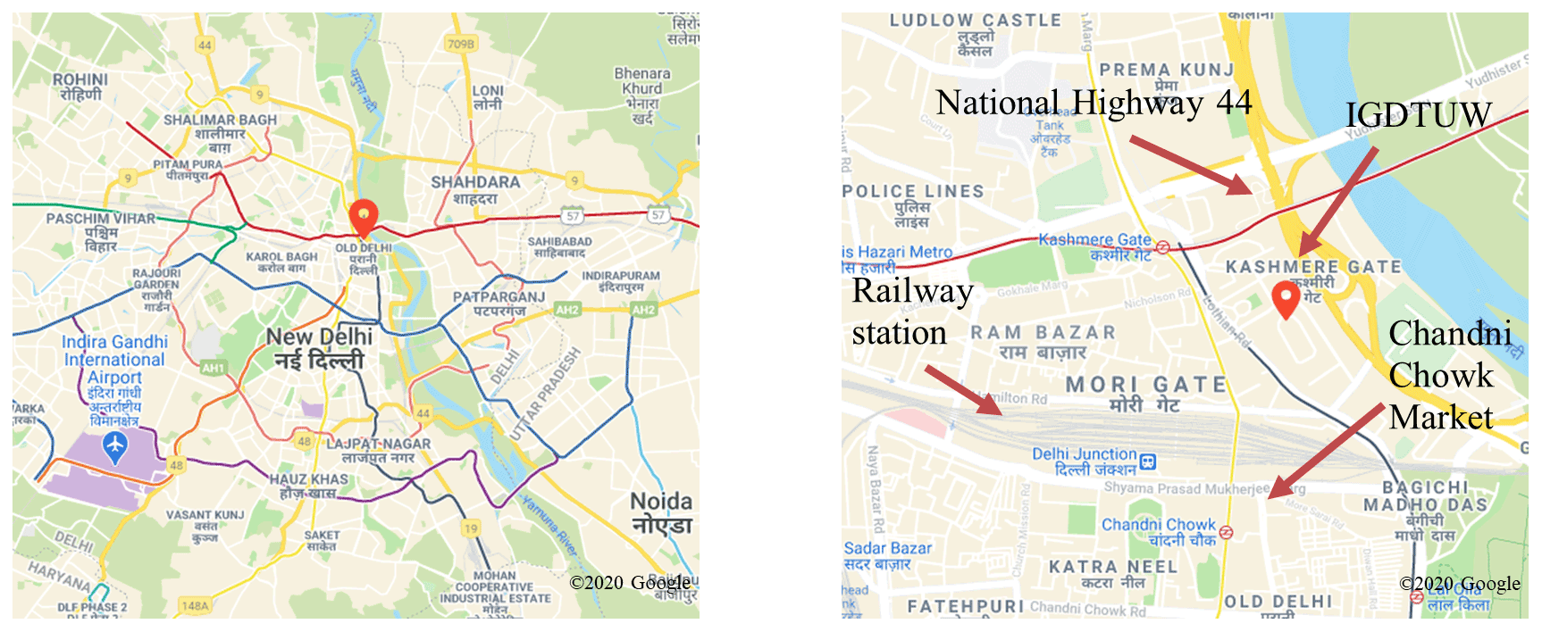
Figure 1 The measurement site (IGDTUW) in Old Delhi, north of New Delhi (left). In closer detail (right), the site was just north of the Delhi Junction Railway Station, and west of National Highway 44. Map data © Google Maps 2020.

2.2 VOC and o-VOC measurements

Two gas chromatography (GC) instruments and a proton transfer reaction time-of-flight mass spectrometer, with quadrupole ion guide (PTR-QiTOF, Ionicon Analytik, Innsbruck) were deployed to measure an extensive range of VOCs and o-VOCs. GC instrumentation included a dual-channel gas chromatography flame ionisation detector, (DC)-GC-FID, measuring C₂–C₈ hydrocarbons and some o-VOCs, and a two-dimensional GC flame ionisation detector (GC × GC-FID) to measure larger hydrocarbon species (C₆–C₁₃). PTR-QiTOF measurements of a variety of o-VOCs completed the VOC measurement suite of 15 alkanes, 10 alkenes, 2 alkynes, 29 aromatics, 11 carbonyls, 2 alcohols, and 15 monoterpenes (see Table S1 in the Supplement). All three instruments operated between 11 and 27 October 2018. The two GC instruments shared an inlet, located approximately 5 m above ground level. The sample line from the inlet to the laboratory was made from $\mathrm{1}/\mathrm{2}$ in. O.D. (9.53 mm I.D.) perfluoroalkoxy (PFA) and was heated to limit adsorption of compounds to surfaces. VOCs and o-VOCs were calibrated using 4 ppbV and a 4 ppmV (diluted before calibration) gas standard cylinders (National Physical Laboratory, UK) respectively, containing a variety of VOCs and o-VOCs. The linearity of the detector response to higher mixing ratios was tested on both instruments prior to the campaigns, as described by Stewart et al. (2021a).

The (DC)-GC-FID measurement period was 5 October–27 October 2018. A 500 mL sample pre-purge (flow rate of 100 mL min⁻¹ for 15 min) preceded a 500 mL sample collection (flow rate of 25 mL min⁻¹ for 20 min) using a Markes International CIA Advantage. The sample was passed through a cold glass finger (−30 ^∘C) to remove water, before being adsorbed onto a Markes International Ozone Precursor dual-bed sorbent cold trap using a Markes International Unity 2 for pre-concentration. After sampling, the trap was heated (250 ^∘C for 3 min) to allow for thermal desorption of the sample and passed to the GC oven in helium carrier gas. The sample was split 50 : 50 and injected into two columns in the oven, allowing for the detection of both non-oxygenated (10 m × 0.53 mm LOWOX column) and oxygenated (50 m × 0.53 mm Al₂O₃ PLOT column) VOCs. The oven was held at 40 ^∘C for 5 min, then ramped up to 110 ^∘C at a rate of 13 ^∘C min⁻¹, before a final ramp to 200 ^∘C at 7 ^∘C min⁻¹, where it was held for 30 min (Hopkins et al., 2003).

The GC × GC-FID measurement period was 11 October–4 November 2018. A 2.1 L sample (flow rate 70 mL min⁻¹ for 30 min) was collected and passed through a cold glass finger (−30 ^∘C) to remove water. The sample was absorbed onto a TO-15/TO-17 air toxic cold sorbent trap in a Markes International Unity 2 for pre-concentration. The trap was heated (250 ^∘C for 5 min) to allow for thermal desorption and the sample injected down a transfer line. It was then refocused with liquid CO₂ at the head of a non-polar BPX5 column (SGE Analytical, 15 m × 0.15 µm × 0.25 mm) held at 50 psi for 60 s. This was connected to a polar BPX50 column (SGE Analytical 2 m × 0.25 µm × 0.25 mm) held at 23 psi via a modulator held at 180 ^∘C (5 s modulation, Analytical Flow Products MDVG-HT). The oven was held for 2 min at 35 ^∘C, then ramped up to 130 ^∘C at a rate of 2.5 ^∘C min⁻¹ and held for 1 min before a final ramp to 180 ^∘C at 10 ^∘C min⁻¹ where it was held for 8 min (Dunmore et al., 2015; Stewart et al., 2021a).

The PTR-QiTOF-MS operated from 4 October–4 November 2018 at a flow rate of 20 L min⁻¹, subsampling from the same inlet line as the GCs. The drift tube pressure and temperature were 3.5 mbar and 60 ^∘C, respectively, giving an $E/N$ (the ratio between electric field strength, E, and buffer gas density, N, in the drift tube) of 120 Td. The PTR-QiTOF-MS subsampled from a $\mathrm{1}/\mathrm{2}$ in. PFA inlet line positioned 5 m above ground next to the inlet used by the GC instruments. The PTR-QiTOF-MS was calibrated daily using a calibration gas (Apel-Riemer Environmental Inc., Miami) containing 18 compounds: methanol; acetonitrile; acetaldehyde; acetone; dimethyl sulfide; isoprene; methacrolein; methyl vinyl ketone; 2-butanol; benzene; toluene; 2-hexanone; m-xylene; heptanal; α-pinene; 3-octanone and 3-octanol at 1000 ppbV (±5 %); and β-caryophyllene at 500 ppbV (±5 %), diluted dynamically into zero air. More details on the PTR-QiTOF-MS can be found in Jordan et al. (2009).

2.3 Measurements of NO_x, CO, SO₂, O₃, and HONO

Measurements of nitrogen oxides (NO_x) were made using a dual-channel chemiluminescence instrument (Air Quality Designs Inc., Colorado, USA), and carbon monoxide (CO) was measured with a resonance fluorescent instrument (Model Al5002, Aerolaser GmbH, Germany). Both instruments were calibrated every 2–3 d throughout the campaign using standard gas cylinders from the National Physical Laboratories, UK. O₃ was measured using an ozone analyser (49i, Thermo Scientific) with a limit of detection of 1 ppbV. The instrument setup and calibration methodology are as described by Squires et al. (2020). An SO₂ analyser (43i, Thermo Scientific) with a limit of detection of 2 ppbV was used to provide measurements of SO₂. HONO was measured with a commercially available long-path absorption photometer (LOPAP) described in Heland et al. (2001) according to the standard procedures outlined in Kleffmann and Wiesen (2008), with baseline measurements taken at regular intervals (8 h). In this study, HONO was also recorded using the PTR-QiTOF-MS with the protonated HONO ion observed at $m/z$ 48.007. This signal was humidity corrected and calibrated against the LOPAP HONO measurements. HONO measurements using PTR-MS have been reported previously in Koss et al. (2018) and are described in more detail in Crilley et al. (2021).

2.4 Measurement of photolysis rates

The model was constrained with the measured photolysis frequencies j(O¹D), j(NO₂), and j(HONO), which were calculated from the measured wavelength-resolved actinic flux and published absorption cross sections and photodissociation quantum yields (Whalley et al., 2021). All other photolysis rates are parameterised as a function of solar zenith angle using a two-stream isotropic scattering model as described by Jenkin et al. (1997) and Saunders et al. (2003). In each case, clear-sky variation of a specific photolysis rate (j) with solar zenith angle (χ) can be described well by Eq. (1):

$$\begin{array}{}\text{(1)}& j=l\cos \left(\mathit{\chi }\right)m\times e-n\sec \left(\mathit{\chi }\right),\end{array}$$

where the parameters l, m, and n optimised for each photolysis rate (see Table 2 in Saunders et al., 2003, and http://mcm.york.ac.uk/parameters/photolysis_param.htt, last access: March 2020).

For species which photolyse at near-UV wavelengths (< 360 nm), such as HCHO and CH₃CHO, the photolysis rates were calculated by scaling to the ratio of clear-sky j(O¹D) to observed j(O¹D) to account for attenuation by clouds and aerosol. For species which photolyse further into the visible, the ratio of clear-sky j(NO₂) to observed j(NO₂) was used.

2.5 Model description

A tailored zero-dimensional chemical box model of the lower atmosphere, incorporating a subset of the Master Chemical Mechanism (MCM v3.3.1; Jenkin et al., 2015) into the AtChem2 modelling toolkit (Sommariva et al., 2020), was used to identify the main drivers of in situ O₃ production, P(O₃), in Delhi. The MCM describes the detailed atmospheric chemical degradation of 143 VOCs, though 17 500 reactions of 6900 species. More details can be found on the MCM website (http://mcm.york.ac.uk, last access: March 2020). Observations of 86 unique VOCs, NO_x, CO, SO₂, and total aerosol surface area (ASA), along with 34 observationally derived photolysis rates, temperature, pressure, and relatively humidity, were averaged or interpolated to 15 min data and used to constrain the model. Some measured VOCs are not described in the MCM. For these species, an existing mechanism in the MCM was used as a surrogate mechanism. Surrogate species were selected based on their structural similarly to the species of interest, and reaction rates with OH, HO₂ and NO₃ were amended to values found in the IUPAC atmospheric chemical kinetics database (Atkinson et al., 2006) and Atkinson and Arey (2003) (see Table S1 in the Supplement). A fixed deposition rate of $\mathrm{1.2}\times {\mathrm{10}}^{-\mathrm{5}}$ s⁻¹ was used, giving model-generated species a lifetime of approximately 24 h.

The model was constrained to an adjusted value of the observed HONO to account for high surface concentrations and an expected decline in concentration with height. The rate of vertical transport of chemical species through turbulence, or Deardorff velocity (w^∗), was calculated during a 2-week follow-on chemical flux campaign in early November 2018 at IGDTUW, after the ground-level measurement period ended. Measurements made from a 30 m tower allowed for the calculation of w^∗, from which an hourly averaged diel has been used to determine an approximate rate of vertical HONO transport. Observed HONO concentrations ([HONO]_meas) were converted to an adjusted HONO concentration ([HONO]_input) with Eq. (2):

$$\begin{array}{}\text{(2)}& [\mathrm{HONO}{]}_{\mathrm{input}}=[\mathrm{HONO}{]}_{\mathrm{meas}}{e}^{-j\left(\mathrm{HONO}\right)t},\end{array}$$

where t is calculated as the time for [HONO]_meas to travel to half the boundary layer height at the measured Deardorff velocity, w^∗. The first-order loss of HO₂ to aerosol surface area (k) was calculated with Eq. (3).

$$\begin{array}{}\text{(3)}& k={\displaystyle \frac{\mathit{\omega }A\mathit{\gamma }}{\mathrm{4}}},\end{array}$$

where ω is the mean molecular speed of HO₂ (equal to 43 725 cm s⁻¹ at 298 K), γ is the aerosol uptake coefficient (0.2 is used here as recommended by Jacob, 2000), and A is the measured aerosol surface area in cm² cm⁻³ calculated (as NSD ⋅ π ⋅ d²) from hourly number size distributions (NSDs). Aerodynamic diameter NSDs, N_a (>352 nm), were collected using a GRIMM 1.108 (portable laser aerosol spectrometer and dust monitor) and merged into concurrently measured electric mobility diameter NSD, N_d (14–640 nm – measured using a TSI scanning mobility particle sizer (SMPS), consisting of a 3080 Electrostatic Classifier, 3081 differential mobility analyser (DMA), and 3775 condensation particle counter (CPC)) using the algorithm developed by Beddows et al. (2010).

The base reference model was run for 5 d, with each day being constrained to the diel campaign-averaged observations, to allow for the spin-up of model-generated species. Only the fifth day was taken for analysis to ensure steady state was reached. A range of additional modelling scenarios, based on this base model, were used to investigate the sensitivity of O₃ production, P(O₃), to changes in VOCs, NO_x, aerosol surface area, and/or photolysis rates:

• Scenario 1: vary both total VOC and NO_x by a factor. VOC and NO_x observations were multiplied by a factor of 0.01, 0.1, 0.25, 0.5, 0.75, 0.9, 1.1, 1.25, 1.5, 1.75, and 2.

• Scenario 2: vary individual primary VOCs and NO_x by a factor. A VOC of interest and NO_x observations were multiplied by a factor of 0.01, 0.1, 0.25, 0.5, 0.75, 0.9, 1.1, 1.25, 1.5, 1.75, and 2. Observed carbonyls (all oxygenated compounds excluding alcohols) were not constrained in this scenario to allow for secondary compounds to be varied with changes in concentrations of their precursor VOC.

• Scenario 3: vary by VOC class and vary NO_x. Individual VOC classes were multiplied by a factor of 0.2, 0.4, 0.6, 0.8, 1.2, 1.4, 1.6, 1.8, and 2. NO_x was multiplied by a factor of 0.25, 0.5, and 0.75. All possible combinations of altered VOC class and NO_x observations were constrained in the model. The remaining VOCs not grouped into the class of interest are constrained at their observed values. Observed carbonyls are not constrained in this scenario to allow for secondary compounds to be varied with changes in concentrations of their precursor VOC.

• Scenario 4: increase individual VOC of interest by 5 %. The constrained concentration of a VOC species of interest was increased by 5 % by molar mass following the procedure carried out in Elshorbany et al. (2009). Comparison of the change in P(O₃) against the base model allows for the determination of ΔP(O₃)_increm (Sect. 3.4). Observed carbonyls are not constrained in this scenario to allow for secondary compounds to be varied with changes in concentrations of their precursor VOC.

• Scenario 5: vary ASA. ASA was multiplied by a factor of 0.1, 0.3, 0.5, 0.7, 0.9, 1.1, 1.3, 1.5, 1.7, 1.9, and 2. The difference in P(O₃) between each model and the base model was examined.

• Scenario 6: vary photolysis rates. All 34 photolysis rates were multiplied by a factor of 0.1, 0.3, 0.5, 0.7, 0.9, 1.1, 1.3, 1.5, 1.7, 1.9, and 2. The difference in P(O₃) between each model and the base model was examined.

• Scenario 7: vary both individual primary VOCs and NO_x by Emissions Database for Global Atmospheric Research (EDGAR) source sector. VOCs were grouped and observed concentrations were divided into each source sector as described by the EDGAR v5.0 Global Air Pollutant Emissions and EDGAR v4.3.2_VOC_spec inventories (https://edgar.jrc.ec.europa.eu/#, last access: November 2020). The proportions of VOC and NO_x concentrations attributed to each individual source were multiplied by a factor of 0.01, 0.1, 0.25, 0.5, 0.75, and 0.9. Observed carbonyls were not constrained in this scenario to allow for secondary production of these compounds to be varied with changes in concentrations of their precursor VOC. For each of these model runs, there were six variations where monoterpenes were assumed to be 0 %, 10 %, 25 %, 50 %, 75 %, and 100 % anthropogenic.

3 Results

3.1 Observed NO_x, CO, and O₃

The observed mixing ratio (ppbV) time series of NO, NO₂, CO, and O₃ during the campaign are presented in Fig. 2. High concentrations of NO and CO were observed towards the latter half of the month, with high daytime O₃ concentrations observed throughout the entire measurement period.

Figure 2 Observed mixing ratio time series of (from top to bottom): NO, NO₂, CO, and O₃ during October 2018.

The diel profile of NO, and to a lesser extent CO, has a U-shaped profile, with much higher concentrations observed at night compared to the day (Fig. 3). This profile results from a shallow and stagnant nocturnal boundary layer, described in more detail in Stewart et al. (2021a). Average daytime concentrations (06:00–18:00 IST, Indian standard time, roughly in line with sunrise and sunset times) of NO and CO were 58.8 ppbV and 1.2 ppmV, respectively. These campaign-averaged diel profiles have large standard deviations, representing the day-to-day variation in concentration throughout October (Fig. 2). Average nighttime concentrations (18:00–06:00) of NO and CO were 247.0 ppbV and 2.9 ppmV, respectively, with NO and CO concentrations occasionally exceeding 800 ppbV and 10 ppmV, respectively, in the latter half of the month (Fig. 2). The NO₂ profile shows two peaks, at approximately 09:00 and 18:00, perhaps due to increased commuting traffic during these times. The O₃ diel profile peaks at approximately 13:00, with a mean peak concentration of 78.3 ppbV. A rapid increase in O₃ concentration is observed first thing in the morning from around 05:00, which levels off at around 06:00 before again rapidly increasing from 08:00 to a peak concentration ∼ 13:00. As the precursor species of O₃ depend on light to undergo the chemical processing that leads to O₃ production, this profile suggests that as the Sun rises rapid photochemical formation of O₃ is initiated by the photolysis of precursors that have accumulated in the lower atmosphere during the nighttime. The early morning increase in O₃ concentrations may also be influenced by the reduced NO titration as the boundary layer height increases (Fig. 3).

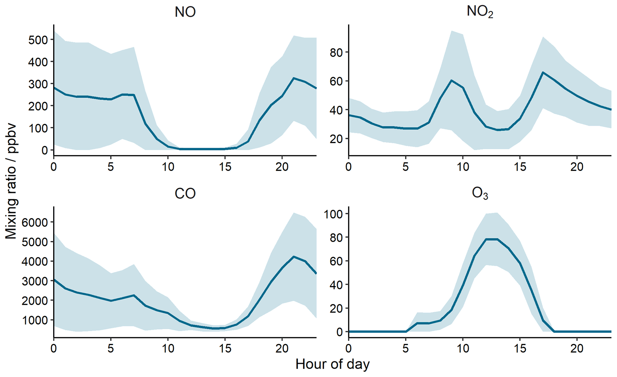
Figure 3 October campaign-averaged diel profiles. The shaded ribbon represents the standard deviation of this average.

Average mixing ratios of NO_x and VOCs observed during the post-monsoon Delhi campaign are comparable to those observed in 1970s Los Angeles. High concentrations of NO_x (∼ 200 ppbV) and VOCs (e.g. benzene ∼ 10 ppbV; toluene ∼ 30 ppbV) led to large concentrations of O₃ in the US city, averaging at around 400 ppbV (Pollack et al., 2013). Despite the high O₃ concentrations observed in Delhi, O₃ concentrations in post-monsoon Delhi did not exceed 150 ppbV and are of similar magnitude to observed O₃ in Beijing, Shanghai, and Guangzhou despite much higher observed VOC and NO_x concentrations (Tan et al., 2019). The lower O₃ observed in Delhi compared to 1970s Los Angeles can be attributed to differences in both topography and meteorology. The isolated coastal city of Los Angeles is surrounded by mountains to the north and east, with the prevailing wind dominating from the coast. Due to its basin-like topography, and with a cool onshore sea breeze often creating a temperature inversion, the air mass circulates within the city and the transport of emissions out of the basin is impeded. Although landlocked Delhi lies to the southwest of the Himalaya, the city is very flat and resides far enough away from the mountain range to allow for the efficient transportation of air masses from the city. It is also important to consider that the very high concentrations of NO_x and VOCs observed peak to comparable concentrations to Los Angeles during the evening and at night, where they are trapped due to a shallow, stagnant boundary layer, and there is little to no photochemical activity. O₃ production rates in Delhi peak in the morning, when concentrations of pollutants, though still high, are much lower than at night due to rapid boundary layer expansion (see Sect. 3.4).

Although 12 key air pollutants, including O₃, have prescribed national ambient air quality standards (Dube, 2009), only four have been identified for regular and continuous monitoring: sulfur dioxide (SO₂), nitrogen dioxide (NO₂), respirable suspended particulate matter (RSPM, or PM₁₀), and fine particulate matter (PM_2.5). The prescribed national standards for O₃ are an 8-hourly limit of 100 µg m⁻³ (∼ 50 ppbV) and 1-hourly limit of 180 µg m⁻³ (∼ 90 ppbV). The observed O₃ 8 h averages between 09:00 and 17:00 throughout the measurement period are shown in Fig. 4, along with the hourly averaged maximum O₃ concentrations.

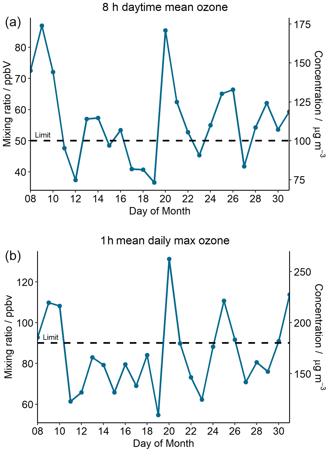
Figure 4 The 8 h mean O₃ concentration between 09:00 and 17:00 IST (a) and hourly averaged maximum daily O₃ concentration (b) during October 2018. The dashed black line shows the prescribed national standards for O₃.

Our observations show that the 8 h O₃ prescribed national standard is exceeded on 16 d during our 24 d measurement period (67 % of days), and the 1 h max is exceeded on 8 d (33 % of days). The published national standards state that any pollutant which exceeds the prescribed values for two consecutive days qualifies for regular and continuous monitoring. As there are up to four consecutive days in which the 8 h daytime mean O₃ limit was breached during our campaign, this implies that O₃ should be continuously and regularly monitored in this part of Old Delhi.

3.2 Observed VOCs

Alkanes were the predominant VOC class contributing to the total measured VOC mass concentration (42 %), consistent with previous observations at the site (Shivani et al., 2018), followed by alcohols (18 %), aromatics (17.8 %), and carbonyls (13.9 %). The percentage contributions of each VOC class to total measured VOCs, along with mean mass concentrations of the top 10 contributors, are presented in Fig. 5. The top individual species contributing to the VOC mass concentrations were ethanol (10.7 %), n-butane (9.9 %) and n-propane (7.9 %).

Figure 5 Percentage contribution of different VOC classes to the total mean measured NMVOCs (a) and the mean concentrations of the top 10 contributors to total measured VOC concentrations (b) during the campaign in µg m⁻³. Colours correspond to the different VOC classes.

The general diel profile for all VOCs, excluding isoprene and some oxygenated species, is U-shaped (Fig. 6). This U-shaped profile is also observed for NO and CO. Concentrations are much higher during the night, and lower in the day, as they are concentrated in a stagnant, shallow boundary layer that forms over the city at night (Stewart et al., 2021a), and are subject to photochemical losses during the day. The U shape is less apparent for acetone, methanol, and ethanol. This may be a result of very high emissions of these compounds during the day and/or formation through secondary chemistry (Stewart et al., 2021a). Isoprene has a typical biogenic diurnal profile, in contrast to monoterpenes which have a similar trend to other anthropogenic species (see α-terpinene, Fig. 6). A separate study which conducted PMF analysis on the co-located PTR-QiTOF flux measurements, resolved two traffic-related factors (Cash et al., 2021). A large proportion of the total measured monoterpenes were resolved within traffic factors (∼ 60 %) and traffic emissions dominated throughout the campaign (∼ 50 % of total VOC emissions). Gkatzelis et al. (2021) have recently shown that monoterpene measurements in New York City can be predominantly apportioned to fragranced volatile consumer products (VCPs) and other anthropogenic sources (e.g. cooking and building materials), and that although biogenic sources are the dominant source of monoterpenes globally, in urban environments monoterpene fluxes from fragranced VCPs can compete with the emissions from local vegetation (see Sect. 3.8 for further discussion of anthropogenic sources of monoterpenes).

The standard deviation of all the aggregate VOC diel profiles is large due to large variations in concentrations from day to day throughout the month. Generally, high concentrations of all species are observed at the end of October and lower concentrations at the start (see Figs. S1 and S2 in the Supplement).

Figure 6 Mean campaign-averaged diel mixing ratio profiles of selected VOCs during the campaign: ethane, ethene, n-butane, isoprene, benzene, α-terpinene, methanol, ethanol, acetone. The shaded ribbon represents 1 standard deviation from the mean. Colours correspond to the different VOC classes.

3.3 OH reactivity, k(OH)

Speciated VOC concentrations alone do not indicate which individual compounds are important for O₃ formation. It is crucial to account for their reactivities with atmospheric oxidants, and their structure, to gain insight into each individual species and compound class contribution to in situ P(O₃). All VOCs react with OH, leading to peroxy radical formation. These peroxy radical species (HO₂ and RO₂) mediate the conversion of NO to NO₂, leading to P(O₃) (Reactions R1–R4). The rate at which VOCs react with OH is thus the rate-determining step in the amount of O₃ formed.

The chemical box model described in Sect. 2.5 was used to investigate the total OH reactivity, expressed as k(OH) – a first-order loss rate in units of s⁻¹, of observed precursors to O₃ (base reference model). NO_x, CO, and individual VOC class contributions to k(OH) are presented in Fig. 7, along with the k(OH) of unmeasured species generated by the model (referred to as “model-generated species” from now on). VOCs and model-generated species represented 67.4 % of the total k(OH), with alkenes (9.6 %) and aromatics (8.8 %) being the largest VOC class contributors. The k(OH) value was higher during the night, showing an inverse relationship with boundary layer height. This is typical for urban environments where nighttime emissions are typically released into a shallow boundary layer (discussed further in Stewart et al., 2021a).

Nighttime boundary layer heights in Delhi were very low, leading to a clearly defined k(OH) profile with a maximum of ∼ 250 s⁻¹ at around 21:00 and a minimum of ∼ 57 s⁻¹ at 14:00. The campaign average boundary layer height range was approximately 39–1550 m. Generally, k(OH) in megacities is found to peak at around 06:00, consistent with morning emissions into a shallow boundary layer. A small peak is also observed around this time in Delhi, but the largest peak is calculated at around 21:00. NO_x represents ∼ 35 %–40 % of the total k(OH) at these times, perhaps due to high volumes of traffic. This is supported by VOC traffic PMF factors described in Cash et al. (2021), which peaks during the evening (∼ 19:00–21:00), and account for ∼ 87 % of the total emissions at this time.

The values of k(OH) determined in this work are significantly higher than those observed in other megacities, with a daytime minimum k(OH) more than double that observed in Beijing during the summer of 2017 (Whalley et al., 2021). Previous studies in New York City, Mexico City, and Tokyo have observed k(OH) > 100 s⁻¹ (Ren et al., 2006; Shirley et al., 2006; Yoshino et al., 2006). A maximum summertime k(OH) of 116 s⁻¹ was observed in London during rush hour, but lower OH reactivities of 22–37 s⁻¹ were more typical during the campaign (Whalley et al., 2016). In a study during summertime in Seoul, average k(OH) was approximately 15 s⁻¹ in the afternoon, increasing to 20 s⁻¹ at night (Kim et al., 2016). High OH reactivities were observed in the Pearl River Delta, with mean maximum reactivities of 50 s⁻¹ at daybreak, and mean minimums of 20 s⁻¹ observed at noon (Lou et al., 2010). Average summertime k(OH) observations from Beijing, China, observed a k(OH) maximum of ∼ 37 s⁻¹ at around 06:00 and daily minimum of k(OH) ∼ 22 s⁻¹ at 15:00 (Whalley et al., 2021), within a boundary layer range of approximately 150–1500 m.

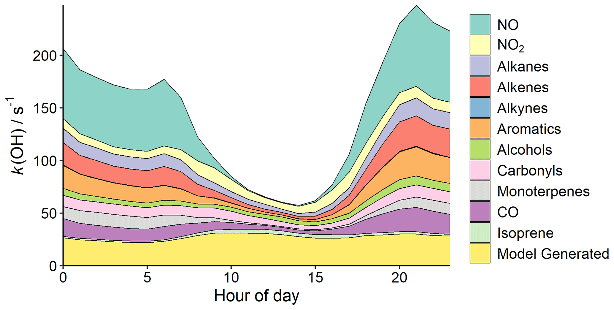
Figure 7 Diel profile of campaign-averaged VOCs, CO, and NO_x contributions to OH reactivity, k(OH).

In Delhi, O₃ concentrations rapidly increase from ∼ 08:00, peaking around ∼ 13:00 before declining in the afternoon (Fig. 3). A breakdown of the percentage contribution of each species class to morning k(OH) (08:00–12:00) is presented in Fig. 8. The average morning k(OH) is dominated by model-generated species (31.9 %), followed by NO_x (21.5 %) and carbonyls (9.2 %).

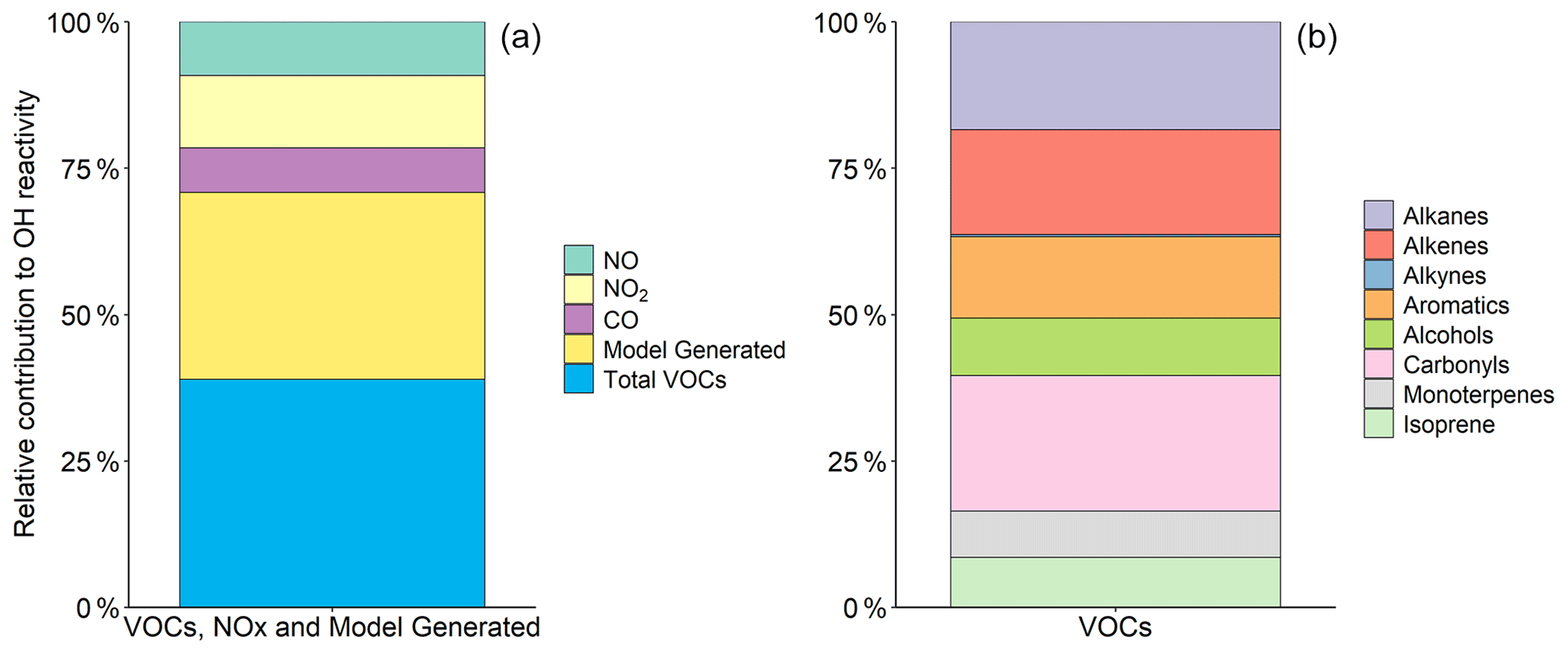
Figure 8 Relative contribution of species classes to average morning OH reactivity, k(OH), (08:00–12:00). The contribution of each group to the total k(OH) including NO_x and model-generated species (a) and the contribution of each class to just the VOC proportion of k(OH) (b).

3.4 O₃ production potentials

Model-generated species are the products of reactions of VOCs of all classes, meaning the overall contribution of individual classes of VOCs to k(OH) is underestimated in Figs. 7 and 8 (Sect. 3.3). To assess the true contribution of VOCs to k(OH) and production, several model runs where each constrained VOC class was increased by 5 % were compared to the base reference model (scenario 4, Sect. 2.5).

One way to assess the contributions of different VOCs to O₃ production is to determine the change in O₃ production, ΔP(O₃), when the base reference model is compared to an adapted model where the VOC of interest is increased by 5 % (Elshorbany et al., 2009). The additional P(O₃) resulting from the 5 % perturbed system was averaged over 24 h. For both the base and 5 % scenarios, the net rate of O₃ production, P(O₃), is calculated by subtracting the instantaneous rate of O₃ loss, L(O₃)_inst, by the instantaneous rate of O₃ production, P(O₃)_inst, via Eqs. (4)–(6). P(O₃)_inst was calculated by determining the NO₂ production rate through reactions of NO with HO₂ and RO₂ (Whalley et al., 2018), assuming the production of a molecule of NO₂ equates to the production of a molecule of O₃ via Reaction (R5). NO₂ loss processes which do not yield O₃, such as removal by reaction with OH and reaction with acyl peroxy radicals to form peroxy acetyl nitrates (PANs), must also be accounted for. In these calculations, OH, HO₂, and RO₂ concentrations are generated from the observationally constrained model.

P(O₃)_inst is the rate of NO oxidation by HO₂ and RO₂ radicals:

$$\begin{array}{}\text{(4)}& \begin{array}{rl}P({\mathrm{O}}_{\mathrm{3}}{)}_{\mathrm{inst}}& =(k_{{\mathrm{HO}}_{\mathrm{2}}+\mathrm{NO}}\left[{\mathrm{HO}}_{\mathrm{2}}\right]\left[\mathrm{NO}\right]\\ & +\sum _i{k}_{{{\mathrm{RO}}_{\mathrm{2}}}_i+\mathrm{NO}}\left[{\mathrm{RO}}_{\mathrm{2}}\right]\left[\mathrm{NO}\right]).\end{array}\end{array}$$

L(O₃)_inst is the rate of loss of O₃ though reactions with OH, HO₂, and photolysis followed by a reaction with H₂O vapour, along with the loss of NO₂ through reactions with OH:

$$\begin{array}{}\text{(5)}& \begin{array}{rl}L({\mathrm{O}}_{\mathrm{3}}{)}_{\mathrm{inst}}& =j\left({\mathrm{O}}^{\mathrm{1}}\mathrm{D}\right)\left[{\mathrm{O}}_{\mathrm{3}}\right]\cdot f+k_{\mathrm{OH}+{\mathrm{O}}_{\mathrm{3}}}\left[\mathrm{OH}\right]\left[{\mathrm{O}}_{\mathrm{3}}\right]\\ & +k_{{\mathrm{HO}}_{\mathrm{2}}+{\mathrm{O}}_{\mathrm{3}}}\left[{\mathrm{O}}_{\mathrm{3}}\right]\left[{\mathrm{HO}}_{\mathrm{2}}\right]\\ & +k_{\mathrm{OH}+{\mathrm{NO}}_{\mathrm{2}}+M}\left[{\mathrm{NO}}_{\mathrm{2}}\right]\left[\mathrm{OH}\right]\left[M\right]\\ & +\sum _i{k}_{{{\mathrm{RO}}_{\mathrm{2}}}_i+{\mathrm{NO}}_{\mathrm{2}}+M}\left[{\mathrm{RO}}_{\mathrm{2}}\right]\left[{\mathrm{NO}}_{\mathrm{2}}\right]\left[M\right],\end{array}\end{array}$$

where f is the fraction of O(¹D) atoms (formed in the photolysis of O₃) that react with H₂O vapour to form OH, rather than undergo collisional stabilisation. Net O₃ production, P(O₃), can then be calculated as

$$\begin{array}{}\text{(6)}& P\left({\mathrm{O}}_{\mathrm{3}}\right)=P({\mathrm{O}}_{\mathrm{3}}{)}_{\mathrm{inst}}-L({\mathrm{O}}_{\mathrm{3}}{)}_{\mathrm{inst}}.\end{array}$$

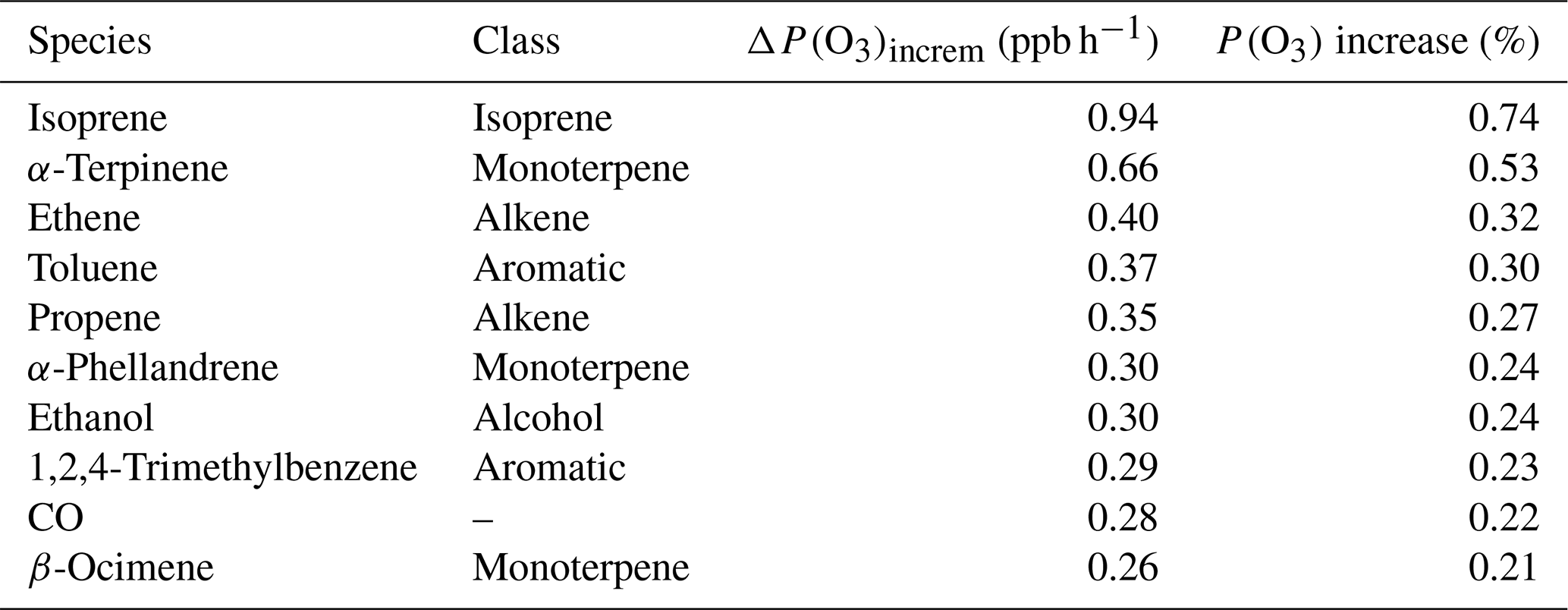
The O₃ production resulting from an incremental increase of each VOC between 08:00 and 12:00, P(O₃)_increm, was then calculated with Eq. (7):

$$\begin{array}{}\text{(7)}& \mathrm{\Delta }P({\mathrm{O}}_{\mathrm{3}}{)}_{\mathrm{increm}}=\mathrm{Mean}(P({\mathrm{O}}_{\mathrm{3}}{)}_i-P({\mathrm{O}}_{\mathrm{3}}{)}_{\mathrm{base}}),\end{array}$$

where P(O₃)_i is the mean O₃ production between 08:00 and 12:00, calculated from the model run where the VOC of interest is increased by 5 %. Using this approach, the 10 VOCs contributing to the greatest change in P(O₃) on an incremental increase, P(O₃)_increm, are isoprene, α-terpinene, ethene, toluene, propene, α-phellandrene, ethanol, 1,2,4-trimethylbenzene, CO, and β-ocimene (Table 1).

Table 1 The top 10 highest ΔP(O₃)_increm VOCs, and their respective classes, averaged between 08:00 and 12:00.

3.5 P(O₃) sensitivities to VOC $/$ NO_x ratios

To better understand the complex non-linear chemistry at play, a box model is used to probe the chemical sensitivities of observed precursors to O₃ formation. The model was run 144 times, each with adjusted concentrations of VOCs and NO_x (scenario 1). The observed concentrations were multiplied by a factor to generate unique model runs from which P(O₃) was calculated using Eqs. (4)–(6). The resultant P(O₃) isopleth is presented in Fig. 9.

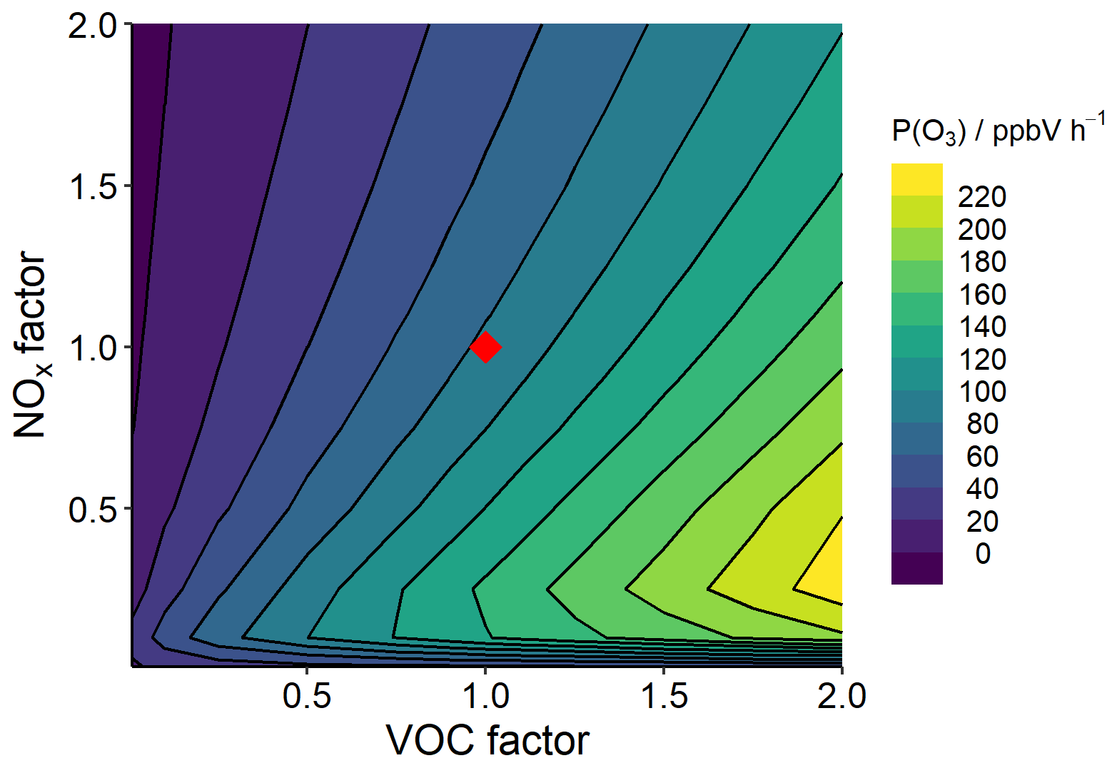
Figure 9 Mean modelled O₃ production, P(O₃), isopleth between 08:00 and 12:00 based on varying VOC and NO_x concentrations in the model. The red diamond at point (1,1) represents modelled P(O₃) at observed VOC and NO_x concentrations.

The modelled VOC–NO_x P(O₃) isopleth supports the assignment of Delhi being, on average, in a VOC-sensitive photochemical regime (Sillman et al., 1990), with the diel profile of O₃ production peaking at 09:00 (see the Supplement, Fig. S3). Reducing NO_x alone and maintaining VOC concentrations would result in an increase in P(O₃). Therefore reducing, or even maintaining, O₃ levels in the future will require a reduction in VOC emissions, if future emission control measures continue to target NO_x emissions in Delhi. This is consistent with a study of observational data in Delhi, whereby a SARS-CoV-2 lockdown led to a reduction in NO_x emissions and concentrations and an increase in the concentration of O₃ (Jain and Sharma, 2020). To implement an efficient and realistic VOC reduction plan, the key VOCs contributing to P(O₃) need to be identified, along with their sources.

As has been previously discussed, O₃ concentrations limits of 50 ppbV were regularly exceeding during the campaign, with the maximum daily 8 h averages peaking at 88 ppbV (Fig. 4). To successfully reduce O₃ to the limit of 50 ppbV, O₃ production must be reduced by 56 %. This can be achieved by reducing NO_x by 25 %, 50 %, and 75 % along with a concurrent reduction in VOCs of 48 %, 61 %, and 78 %, respectively. Alternatively, if VOCs were halved, NO_x reductions could not exceed 29 % to peak O₃ below 50 ppbV. To obtain a reduction in O₃ production without reducing VOCs would require a NO_x reduction of at least 92 %. However, it is important to consider that reducing emissions of NO_x and VOCs by these values will only impact the in situ formation of O₃. Regional O₃ production leading to the transportation of O₃ from outside of Delhi is beyond the scope of this analysis and must also be taken into consideration by policy makers.

3.6 P(O₃) sensitivity to VOCs: by class

The impact of changing VOC concentrations (by class) on mean P(O₃) was investigated using scenario 3 (Sect. 2.5). For each model run, the constrained concentrations of all species in the class of interest were multiplied by a “VOC factor”. Modelled P(O₃) was calculated upon changing “VOC factor” for CO and six different VOC classes: alkanes, alkenes, aromatics, monoterpenes, isoprene, and alcohols. Changes in P(O₃) were found to be most sensitive to changes in aromatics, followed by the monoterpenes and alkenes (Fig. 10). Halving aromatic, monoterpene, and alkene concentrations independently (reducing a VOC factor of 1 to a VOC factor of 0.5, Fig. 10) reduced modelled P(O₃) by 15.6 %, 13.1 %, and 12.9 %, respectively. However, future air quality control strategies are also likely to include a co-reduction in NO_x. As we observed in Fig. 9, a reduction in NO_x coupled with an insufficient reduction in VOCs is likely to increase P(O₃) in Delhi, under VOC-limited conditions. On concurrently reducing VOC class and NO_x by half (factor of 0.5, Fig. 10), aromatics, alkenes, and monoterpenes lead to the smallest increase in P(O₃) (24.9 %, 29.8 %, and 35.5 % respectively). However, this still represents a significant increase in P(O₃). This suggests targeting one VOC class alone in future pollutant reduction strategies is insufficient, and that reducing a source/sources emitting multiple VOC classes is important to avoid an increase in P(O₃) on simultaneously reducing NO_x.

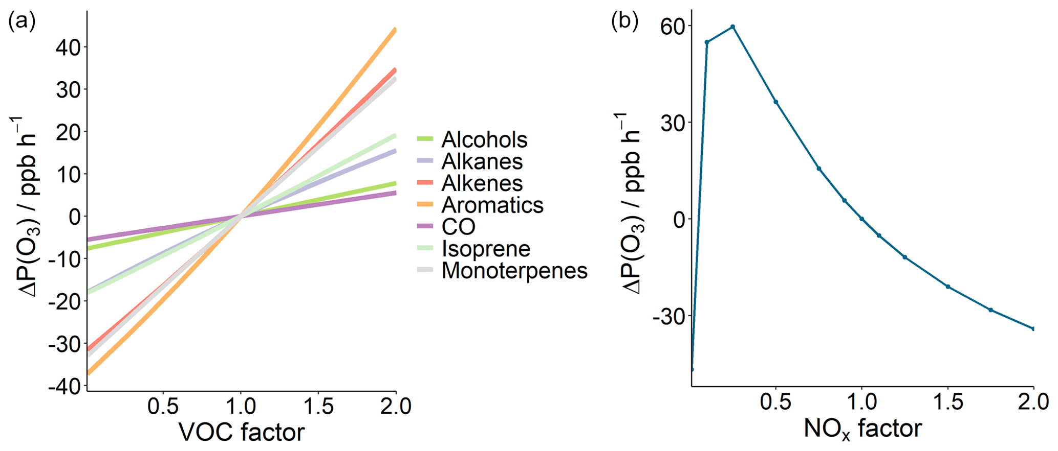
Figure 10 Modelled mean morning (08:00–12:00) change in P(O₃) rate for CO and six VOC classes upon varying their concentrations by multiplying by the “VOC factor” (a) and by varying just NO_x (b).

3.7 The impact of aerosol surface area on P(O₃)

Aerosol particles in the troposphere can impact gas phase chemistry and photochemical activity, affecting P(O₃), in a number of ways. Aerosols can interact with incoming solar radiation, either scattering or absorbing sunlight. The precise impact of aerosol is dependent on a range of factors including chemical composition, particle size distribution, and phase state. It has previously been shown that in highly polluted urban areas, attenuation of the actinic flux due to aerosol absorption can significantly reduce photolysis rates, and hence P(O₃), by up to 30 % (Castro et al., 2001; Hollaway et al., 2019; Real and Sartelet, 2011; Wang et al., 2019). Conversely, aerosol scattering can potentially increase P(O₃) by increasing the photolysis rates (Dickerson et al., 1997; He and Carmichael, 1999).

Aerosol can also participate in heterogeneous chemistry; i.e. uptake of radicals to the aerosol or reactions at the aerosol surface can affect gas phase radical budgets (George et al., 2015). A recent regional modelling study (K. Li et al., 2019) linked increasing O₃ concentration trends between 2013 and 2017 in Beijing to decreasing PM_2.5 concentrations. The study attributed this to the decreased uptake of HO₂ radicals to aerosol particles, leading to increased HO₂ available to participate in P(O₃) (see Reaction R4). However, an experimental study (Tan et al., 2020) in the North China Plain did not observe the effect. The relationship between aerosol optical depth (AOD) and photolysis rates is strongly non-linear and has a larger impact at low solar zenith angles (i.e. in the morning/evening/high latitudes) (Wang et al., 2019).

To investigate the potential impact of aerosol related processes in Delhi, ASA and photolysis rates were varied independently in the model using a scaling factor (“Factor”, Fig. 11), and the resulting impact on P(O₃) calculated. The first-order loss of HO₂ to aerosol surface area (k) was calculated using Eq. (3) (scenario 5, Sect. 2.5).

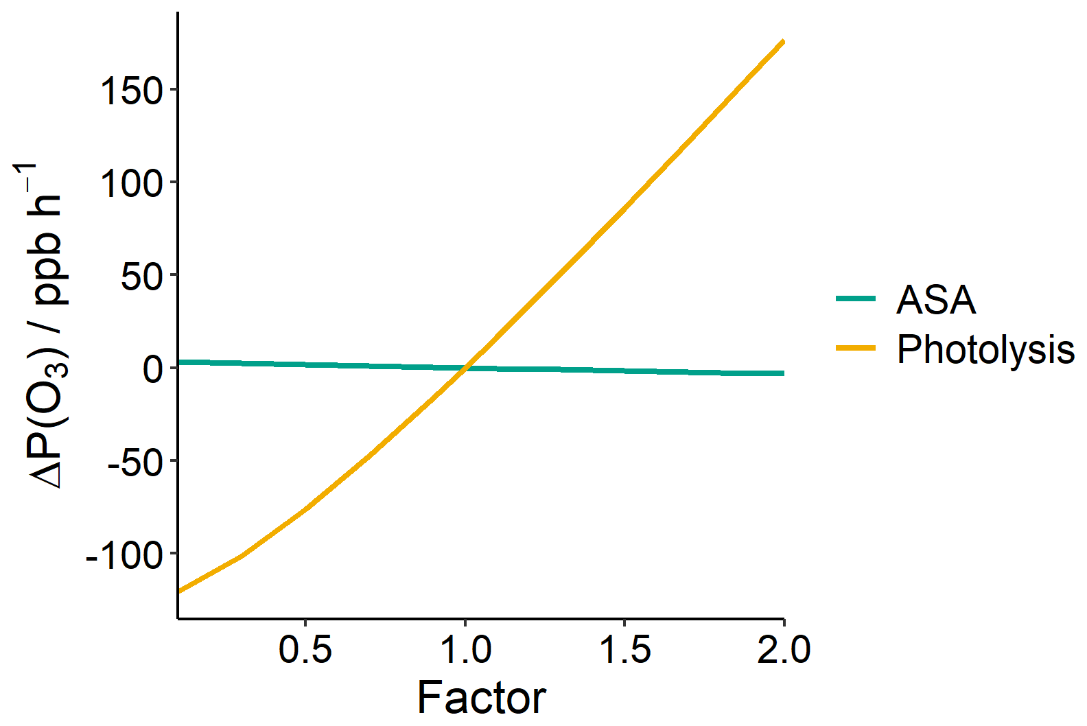
Figure 11 Impact of varying photolysis rates and ASA on mean modelled morning O₃ production rates, ΔP(O₃) (08:00–12:00).

Changes in ASA, with respect to HO₂ uptake, were found to have minimal impact on the modelled mean morning P(O₃) rate (08:00–12:00), as shown in Fig. 11, in line with the observations of Tan et al. (2020). The lifetime of HO₂ is dominated by its reaction with NO, within the campaign-averaged NO concentrations observed. Changes to the photolysis rates have a large impact on P(O₃) (Fig. 11), with P(O₃) increasing roughly linearly with increasing photolysis rates. The impact of changes to AOD on photolysis rates are non-linear and dependent on solar zenith angle (SZA) (i.e. time of day). This work shows that the majority of daily P(O₃) occurs between 08:00 and 12:00, representing an SZA range of 35–80^∘. Aerosol loading is expected to reduce in Delhi going into the future if India implements air pollution controls in line with other countries. Based on the work of Wang et al. (2019), reductions in PM, leading to reductions in AOD, could potentially increase j(NO₂) by up to 30 % at midday and up to 100 % at 08:00. This will lead to increased photochemical activity and higher P(O₃).

From an air quality perspective, it is important to consider reducing not only VOCs but also NO_x concentrations in Delhi. Along with this, reductions in PM should also be considered. As we have seen in Fig. 11, reducing ASA does not significantly impact P(O₃) through heterogenous chemistry. However, an ASA reduction will result in a decrease in AOD, which will in turn increase photolysis rates. A recent study by Chen et al. (2021) modelled the impact of AOD on photolysis in Delhi during November 2018, and found that halving the AOD results in a 14 % increase in j(NO₂). In Delhi, total VOCs would need to be reduced by ∼ 50 % to maintain current P(O₃) rates if NO_x were halved and photolysis rates increased by 14 %. However, the impact of reducing aerosol on photolysis rates is complex. Reductions in aerosol at ground level may lead to either increased or decreased photolysis rates near the surface, depending on the scattering properties of the aerosol. Changes in photolysis rates from increased or decreased aerosol loading may also vary throughout the depth of the boundary layer. The box model assumes photolysis rates are uniform throughout the boundary layer and that aerosols are well mixed. A more detailed study on the temporal and spatial patterns of aerosol in Delhi and its impact on photolysis rates is required to fully assess the aerosol impact on in situ O₃ production (Castro et al., 2001).

It is important to note that this study focuses on the sensitivity of P(O₃) to ASA through HO₂ uptake only. Additional chemical consequences and feedbacks of decreasing aerosol, such as changes to HONO concentrations, have not been accounted for here. With the high levels of NO₂ observed in Delhi, the heterogenous conversion of NO₂ to HONO on particle surfaces may be an important mechanism (Liu et al., 2014; Lee et al., 2016; Tong et al., 2016; Lu et al., 2018b). HONO reductions from decreased ASA may lead to reduced OH radical formation in Delhi; thus, the impact of ASA reduction on P(O₃) may be underestimated in this work.

3.8 Discussion

If future air pollution controls in Delhi follow the air quality strategies prevalent or planned in many other countries, including the EU, there is a danger that urban O₃ concentrations could significantly increase, unless careful consideration is given to the specific atmospheric chemistry occurring in the city. Many other major cities across the globe have focused their air pollution abatement strategies on reducing NO_x and particulate emissions from traffic sources. Urban NO_x emissions (at tailpipe) are likely to decline over time, as a result of improved exhaust gas treatments, the turnover of the fleet to newer, less polluting vehicles, and the increasing prevalence of electric vehicles (Molina, 2021). While this is also likely to reduce ambient VOC concentrations through reduction in tailpipe and evaporative emissions, this reduction may be smaller than for NO_x. The magnitude of resulting changes in P(O₃) from reduced road transport emissions may depend on the proportion of VOCs emitted from road transport relative to other, non-vehicular sources. As demonstrated here, reductions in NO_x without sufficiently reducing VOC emissions may lead to large increases in P(O₃) under a continued VOC-limited regime. Reducing traffic emissions will also likely lead to reduced aerosol loading in Delhi. Our study suggests a reduction in aerosol surface area will have very little direct effect on P(O₃) via heterogenous chemistry, as HO₂ reactivity is dominated by its reaction with NO. However, an ASA reduction is likely to increase the amount of sunlight reaching the boundary layer and hence photolysis rates. This will lead to a subsequent increased P(O₃), as discussed in more detail by Chen et al. (2021).

P(O₃) in Delhi was found to be most sensitive to reductions in aromatics and alkenes, and so monitoring the abundance and knowing the sources of these compounds in Delhi is essential for implementing effective pollutant reduction strategies to avoid a future rise in P(O₃). As these classes are thought to come mainly from traffic sources, it is possible that reducing road transport emissions may reduce traffic-derived VOCs sufficiently, along with reducing NO_x, to perturb a large increase in P(O₃). However, the proportion of VOCs in Delhi, and at IGDTUW, attributed to traffic sources is uncertain, and thus the extent to which road transport reductions will impact P(O₃) is unknown.

More information of the effect of reductions in NO_x and VOCs by source can be obtained by varying sources described by emissions inventories. Anthropogenic emissions of NO_x, CO, and VOCs by source in Delhi are available from the EDGAR v5.0 Global Air Pollutant Emissions and EDGAR v4.3.2_VOC_spec inventories (https://edgar.jrc.ec.europa.eu/#). According to the inventory, all pollutants investigated in this analysis can be almost entirely described by five source sectors (Table 2): road transport (RT); railways, pipelines, and off-road transport (RPORT); energy for buildings (EB); combustion for manufacturing (CM); and process emissions (PE). However, it should be noted here that the EDGAR emissions inventory describes a coarse, low-spatial-resolution city-wide representation of emissions from Delhi. For this analysis, we assume the EDGAR sector split ratios for Delhi are representative of those at the IGDTUW measurement site.

Model-constrained concentrations were varied by their contributions to sources in the EDGAR emissions inventory (scenario 7, Sect. 2.5). Data from the inventory represent average annual emissions from source sectors, last updated for VOCs in 2012 and 2008 for monoterpenes, with 0.1^∘ × 0.1^∘ spatial resolution. VOCs were assumed to be described in full by all sources available from the inventory, with no biogenic influence. Isoprene was excluded from the analysis as it is assumed to have an entirely biogenic source. As a significant anthropogenic signature is seen from the monoterpenes, and because of their significance for P(O₃) in this study, 50 % are assumed to be from anthropogenic sources found in the EDGAR emission inventory for the purpose of this analysis. A full list and description of sources used from the EDGAR inventory can be found in the Supplement. Figure 12 shows the change in P(O₃) rate when reducing VOCs and NO_x contributions from individual source sectors.

Table 2 Relative proportion of pollutants emitted from five EDGAR emission inventory source sectors: road transport (RT); railways, pipelines, and off-road transport (RPORT); energy for buildings (EB); combustion for manufacturing (CM); and process emissions (PE).

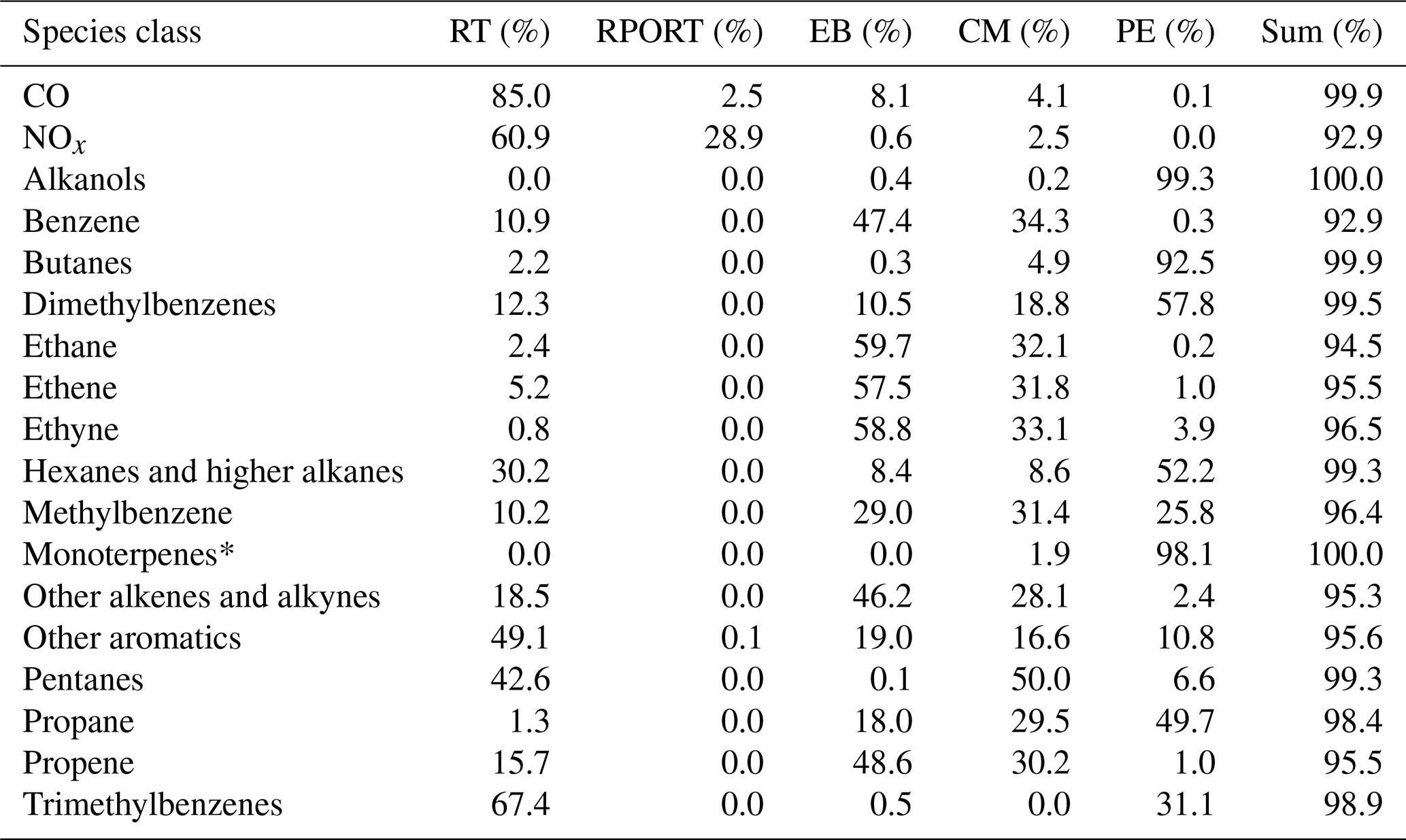
^* The percentage of monoterpenes attributed to these sources in varied in the model and is assumed to be 50 % in the base case.

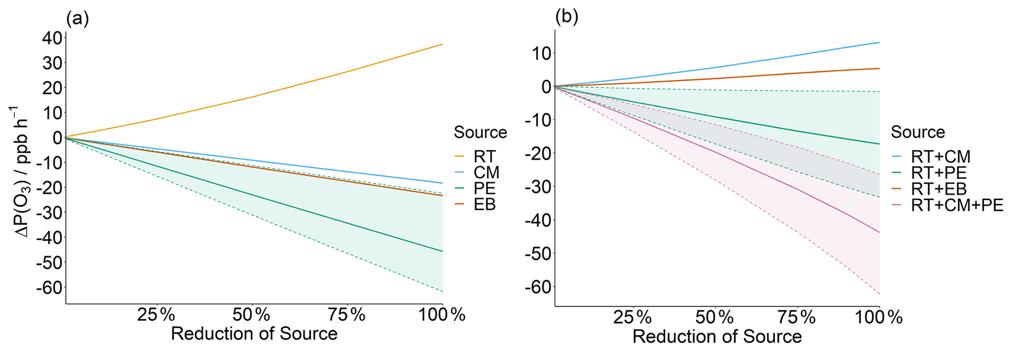
Figure 12 Change in P(O₃) on reducing RT, CM, PE, and EB (a); and (b) reducing road transport simultaneously along with either (i) CM, (ii) PE, (iii) EB, (iii) CM, or PE. The shaded region, bounded by a dashed line, represents the variability in ΔP(O₃) when 0 %–100 % of observed monoterpenes contribute to anthropogenic EDGAR source sectors that include PE. The solid lines represent the base case whereby 50 % of monoterpenes are assumed to be from anthropogenic sources described in the EDGAR inventory (the other 50 % are assumed to be from biogenic sources).

Based on this analysis, reducing the RT source in isolation results in increased P(O₃), whilst reducing CM, PE, and EB independently leads to decreased P(O₃). This is explained by CM, PE, and EB being major sources for VOCs, and RT also being a major source of NO_x. Although reducing RT also reduces some VOCs, particularly aromatic and higher alkane species, there is not sufficient VOC reduction to compensate for the large co-reduction in NO_x, leading to increased P(O₃) (Fig. 10). Reducing RT by 100 % would still lead to a modelled P(O₃) increase of ∼ 40 ppb h⁻¹ (Fig. 12a). It is important to acknowledge the uncertainties in this analysis. The EDGAR emissions inventory attributes a low percentage split of VOCs to the RT source sector at the city level, perhaps underestimating the proportion of VOCs that would be reduced with RT reductions at the measurement site.

Air quality mitigation strategies should therefore focus on reducing RT, alongside one or more additional major VOC sources. For example, Fig. 12b shows P(O₃) begins to reduce when RT emissions are reduced along with PE. These reductions are even greater when RT is reduced with both PE and CM sources. When RT is reduced by 50 % alongside PE and PE + CM, modelled P(O₃) is reduced by ∼ 10 ppb h⁻¹ and ∼ 20 ppb h⁻¹, respectively. The VOCs that contribute the most to PE and CM emissions are n-butane, propane, alcohols, toluene, and xylenes. Although alcohols and alkanes were not identified as the key VOC classes contributing to P(O₃) (Sect. 3.6), they are the two largest classes of VOCs observed in Delhi by mass, making up 42 % and 18 % of the total measured VOCs, respectively (Fig. 5). Reducing the PE source thus leads to large reductions in VOCs by mass, helping to drive down P(O₃). However, it is worth noting that the effectiveness of reducing the RT + PE source on modelled P(O₃) is dependent on the proportion of anthropogenic monoterpene emissions in Delhi. According to the EDGAR emission inventory, 98.1 % of anthropogenic monoterpenes in Delhi are attributed to process emissions (PE) (Table 2). These emissions include sources such as emissions from chemical industry, and other industrial processes, and include solvent emissions and emissions from product use (see Table S3 in the Supplement). As emissions from these sources are grouped together in the EDGAR inventory, the exact sources that monoterpenes are attributed to cannot be identified. The sensitivity of ΔP(O₃) from reducing process emission sources (PE, RT + PE, and RT + PE + CM) is shown by the shaded regions in Fig. 12, where the dashed lines represent the sensitivity limits where the observed monoterpenes are between 0 % and 100 % anthropogenic (as opposed to biogenic). There is relatively little impact on P(O₃) on reducing RT + PE when monoterpenes are assumed to have an entirely biogenic source. However, it is clear that although the degree to which reducing process emissions along with road transport in this study impacts P(O₃) cannot be accurately determined, even if no monoterpenes are reduced within this source, reducing it does not negatively impact P(O₃). It is also important to consider possible underestimations for the monoterpene contribution to RT. Monoterpene observations in Delhi were strongly correlated with CO emissions, suggesting anthropogenic sources (Stewart et al., 2021a). The EDGAR emissions inventory assigns 0 % of the anthropogenic monoterpenes in the inventory to the RT source sector (Table 2). An analysis of the PTR-QiTOF flux data, obtained at the IGDTUW measurement site directly after the concentration measurement period ended, suggests ∼ 60 % of the monoterpenes observed could be attributed to traffic factors (Cash et al., 2021). A study by Wang et al, 2020 suggested vehicular and burning sources may contribute to the anthropogenic emissions of biogenic molecules. Other possible sources of anthropogenic monoterpenes in Delhi are emissions from cooking herbs and spices, and from fragrances and personal care products (Klein et al., 2016; McDonald et al., 2018).

It should be noted that the EDGAR inventory data used in this study are cropped to the Delhi area, and thus some anthropogenic sources may be missing. One example of this is that of agricultural burning, which is frequent in areas surrounding Delhi and across the Indo-Gangetic Plain (IGP) (Jat and Gurjar, 2021; Kulkarni et al., 2020). It is likely that regional sources of O₃ and its precursors will have a significant effect on Delhi's air quality, and vice versa. There are likely to be many missing sources from the EDGAR emissions inventory, along with discrepancies between the top-down and bottom-up data. In addition, we assume the ratios of VOCs and NO_x in each source sector for the Delhi region are representative of the ratios emitted near IGDTUW. Whilst the OH reactivity analysis provides an instantaneous assessment of a VOC's reactivity, based on local observations with a small spatial footprint, the EDGAR Delhi-wide sectoral split represents an aggregate of a wider region and may underrepresent the RT VOC contribution observed at the measurement site. As a result, the magnitude of the modelled increased P(O₃) when road transport is reduced may represent a worst-case scenario.

4 Conclusions

A detailed chemical box model constrained to an extensive observational dataset of 86 VOCs, 34 photolysis rates, NO, NO₂, CO, SO₂, HONO, temperature, pressure, and relative humidity was used to explore the sensitivity of photochemical O₃ production, P(O₃), to VOCs and NO_x in the Indian megacity of Delhi. The urban measurement site at the Indira Gandhi Delhi Technical University for Women is determined to be in a VOC-limited chemical regime. Our analysis examined the sensitivity of VOC classes to mean morning P(O₃), and the aromatic VOC class was identified as being the most important, with a 50 % reduction in ambient concentrations leading to a reduction in modelled morning P(O₃) of 15.6 %, followed by monoterpenes and alkenes (13.1 % and 12.9 %, respectively). The direct impact of the aerosol burden on P(O₃) was found to be negligible with regards to heterogeneous radical uptake. However, P(O₃) was sensitive to increasing photolysis, which may result from decreasing particulate matter that is likely to arise from future emission reduction strategies. Though it is important to reduce NO_x and particulate matter in all abatement strategies, reducing NO_x without reducing VOCs was found to significantly increase P(O₃). VOCs and NO_x were also evaluated by their respective contributions to different source sectors as defined in the EDGAR emissions inventory. Reducing emissions from road transport sources alone led to increased P(O₃), even when the source was removed in its entirety. This suggests a balanced approach to pollution reduction strategies is required, and multiple sources should be targeted simultaneously for effective reduction, incorporating major monoaromatic, alkene, and anthropogenic monoterpene VOC sources. Reducing road transport emissions along with combustion from manufacturing and process emissions was found to be an effective way of reducing P(O₃). Monoterpenes are found to have a significant impact on P(O₃) and showed a diurnal profile consistent with other anthropogenic VOCs. Future work should be carried out to determine the sources and fraction of anthropogenic emissions to the observed monoterpene concentrations measured in Delhi, with a recent study suggesting 60 % of the monoterpenes observed at the site are coming from traffic related sources (Cash et al., 2021). To further understand the complex urban atmospheric chemistry in Delhi, more model constraints are required, such as the measurement of radical species and k(OH). The potential effects of chlorine chemistry were also not investigated in this study and may have an important role in the local chemistry due to the prevalence of waste burning in the city (Gunthe et al., 2021). Satellite observations and aircraft measurements may also help develop our understanding of the regional impacts of regional agricultural biomass burning on Delhi from neighbouring states. This work highlights that a careful approach, considering the complexities of chemical processing in the urban atmosphere, is required for effective air quality improvement strategies.