Influence of sea salt aerosols on the development of Mediterranean tropical-like cyclones

Medicanes are mesoscale tropical-like cyclones that develop in the Mediterranean basin and represent a great hazard for the coastal population. The skill to accurately simulate them is of utmost importance to prevent economical and personal damage. Medicanes are fueled by the latent heat released in the condensation process associated with convective activity, which is regulated by the presence and activation of cloud condensation nuclei, mainly originating from sea salt aerosols (SSAs) for marine environments. Henceforth, the purpose of this contribution is twofold: assessing the effects of an interactive calculation of SSA on the strengthening and persistence of medicanes, and providing insight into the casuistry and sensitivities around their simulation processes. To this end, a set of simulations have been conducted with a chemistry–meteorology coupled model considering prescribed aerosol (PA) and interactive aerosol (IA) concentrations. The results indicate that IA produces longer-lasting and more intense medicanes. Further, the role of the initialization time and nudging strategies for medicane simulations has been explored. Overall, the results suggest that (1) the application of spectral nudging dampens the effects of IA, (2) the initialization time introduces a strong variability in the storm dynamics, and (3) wind–SSA feedback is crucial and should be considered when studying medicanes.

1 Introduction

Mediterranean tropical-like cyclones, also known as medicanes (from mediterranean hurricanes), are mesoscale perturbations that exhibit tropical characteristics, such as an eye-like feature and warm core. These storms are characterized by high wind speeds and vertically aligned geopotential height perturbations along different pressure levels. Just like regular tropical cyclones, medicanes represent a hazard for the population of coastal areas. However, given the relatively small extent of the Mediterranean basin and the lower sea surface temperatures of the Mediterranean Sea, as well as the common presence of environmental wind shear at midlatitudes, they do not reach the size and intensity of actual hurricanes. Still, they can produce heavy precipitation and intense wind gusts, reaching up to Category 1 on the Saffir–Simpson scale (Fita et al., 2007; Miglietta and Rotunno, 2019). Thus, our ability to understand and simulate accurately medicanes with state-of-the-art meteorological modeling systems stands as a key factor to prevent their associated damages.

Tropical-like cyclones in general, and medicanes in particular, are usually considered to be a hybrid between tropical and extratropical cyclones. Although their triggering and early development mechanisms differ from those of tropical cyclones (Tous and Romero, 2013; Cavicchia et al., 2014; Miglietta and Rotunno, 2019; Dafis et al., 2020), such storms are generally maintained in the same way as tropical cyclones in their mature stage: through the evaporation of water from the ocean surface. The initial convective activity caused by potential instability produces the condensation of moist rising air through adiabatic cooling. The condensation process releases latent heat that warms the cyclone core, which is the dominant mechanism that sustains the vortex structure (Lagouvardos et al., 1999).

Numerous studies have addressed the sensitivity of medicane simulations to different factors related to their intensification and track. Some authors have studied the effects of an increased sea surface temperature (SST) (Pytharoulis, 2018; Noyelle et al., 2019), while others focused on the role of air–sea interaction and surface heat fluxes (Tous et al., 2013; Akhtar et al., 2014; Ricchi et al., 2017; Gaertner et al., 2018; Rizza et al., 2018; Bouin and Lebeaupin Brossier, 2020) or the influence of using several different physical parameterizations (Miglietta et al., 2015; Pytharoulis et al., 2018; Ragone et al., 2018; Mylonas et al., 2019). However, less attention has been paid to the microphysical processes and aerosol–cloud interactions, still a great source of uncertainty for understanding convective systems (Fan et al., 2016). In fact, according to the Fifth Report of the Intergovernmental Panel on Climate Change (Boucher et al., 2013), the quantification of cloud and convective effects in models and of aerosol–cloud interactions is still a major challenge. In this type of storms, the microphysics of both cold and warm clouds plays a crucial role. The activation of aerosols as cloud condensation nuclei (CCN), the water absorption during the droplet growth and the auto-conversion processes are main drivers in the core heating and dynamic evolution. In particular, the most common basis of aerosol–cloud interactions, comprised of the Köhler theory, treats the different characteristics of aerosols in terms of size, hygroscopic growth rate and solute mass to determine its activation as cloud condensation or ice nuclei, their later growth as hydrometeors, and their final conversion into raindrops or snow. In this regard, the different consideration of aerosols introduced in different aerosol models largely influences the cloud formation and thus the intensification and evolution of the associated medicane structure. Hence, the use of an appropriate microphysics parameterization, along with the explicit solving of aerosols, seems to be fundamental for the development of the medicanes in the model simulations. Gaining insight into these cloud microphysics processes is a key step for reaching a complete process understanding. In this sense, the working hypothesis in this contribution is that aerosols play a role in a positive feedback with the surface winds that fuel the storm, maintaining its structure and intensity, and thus an interactive calculation of sea salt aerosol (SSA) emissions and concentrations is fundamental for an accurate simulation of the medicane intensification and maintenance (Rizza et al., 2021), as in tropical cyclones (Rosenfeld et al., 2012; Jiang et al., 2019a, b, c; Luo et al., 2019).

In addition, given the high sensitivity of both extratropical (Doyle et al., 2014) and tropical cyclones (Cao et al., 2011) in general, and medicanes in particular (Cavicchia et al., 2014), to the atmospheric configuration, which is fundamental to enable the start of convective activity, the initial conditions feeding the simulations largely impact the medicane development. In consequence, initialization time is an important source of variability (Cioni et al., 2016). In this respect, constraining the synoptic scales to follow reanalysis while allowing the model to develop the small‐scale dynamics, which is exactly the function of spectral nudging, stands as a good method to reduce this variability and effectively constrain the uncertainty of the simulations.

Within this framework, the present contribution aims at analyzing the role played by aerosols in the development of medicanes, together with the influence of the initialization time and the potential benefits or caveats of using nudging techniques for the simulations of these storms.

2 Methods

The results presented below are based on the analysis of an ensemble of 72 simulations, which consist of all the possibilities resulting from the combination of three medicanes (Rolf, Cornelia and Celeno), two nudging configurations (no nudging – NN – and spectral nudging – SN), two configurations for the aerosol concentration calculations (prescribed aerosol and interactively calculated aerosol, hereinafter referred to as PA and IA, respectively), and six run-up times (12, 36, 60, 84, 108 and 132 h).

In this section, the main techniques applied to conduct and analyze the simulations are outlined, along with some details about the model parameterizations and the synoptic conditions associated with the studied events. It also contains a brief explanation of the interactive calculation of the SSA concentration, as included in the meteorology–chemistry coupled mesoscale model WRF-Chem (Weather Research and Forecasting model with Chemistry).

2.1 Model setup

The WRF model (V3.9.1.1) is used to conduct the simulations of this study (Skamarock et al., 2008). The same model configuration is employed for all simulations contained herein unless otherwise indicated. The Morrison et al. (2009) bulk microphysics scheme is used (mp_physics = 10). This scheme allows for a double-moment approach, in which number concentration, along with the mixing ratio, is considered for each hydrometeor species included in the subroutine. In its single-moment version (progn = 0), only the mass (i.e., mixing ratio) is taken into account. Hence, while for the single-moment approach a constant concentration of an aerosol with a prescribed size is used, the second-moment approach introduces the complexity degree of considering a size distribution for the aerosol population, thus being a more realistic approach.

With respect to the physical configuration, radiation is parameterized with the Rapid Radiative Transfer Model for global climate models (RRTMG) by Mlawer et al. (1997), for both short- and long-wave radiation, solved in 30 min intervals. Additionally, the selected option for the surface layer parameterization uses the MM5 (Fifth-Generation Penn State/NCAR Mesoscale Model) scheme based on the similarity theory by Monin and Obukhov (1954), while the Unified NOAH LSM option is used to simulate the land–surface interactions (Mitchell, 2005). The number of soil layers in the land surface model is four. The Yonsei University scheme is employed for the boundary layer (Hong et al., 2006), solved every time step (bldt = 0). For the cumulus physics, the Grell 3D ensemble (cu_physics = 5; cudt = 0) is chosen to parameterize convection (Grell and Dévényi, 2002). Heat and moisture fluxes from the surface are activated (isfflx = 1), as well as the cloud effect to the optical depth in radiation (icloud = 1). Conversely, snow-cover effects are deactivated (ifsnow = 0). Noah-modified 21-category IGBP-MODIS land-use data, land–sea mask topography (Danielson and Gesch, 2011) and soil category data (Dy and Fung, 2016) were obtained from the WRF user's page (WPS, 2019). SST is assimilated from ERA-Interim (sst_update = 1) every 6 h (auxinput4_interval_s = 21 600). The model top is fixed at 1000 Pa, and 40 vertical levels are used for the model runs. The urban canopy model is not considered (sf_urban_physics = 0), and the topographic surface wind correction from Jiménez and Dudhia (2012), later modified by Lorente-Plazas et al. (2015), is turned on. Both feedback from the parameterized convection to the radiation schemes and SST update (every 6 h, coinciding with the update of boundary conditions) are also turned on.

ERA-Interim global atmospheric reanalysis is used to provide the required initial and boundary conditions every 6 h. This dataset comes from the ECMWF’s Integrated Forecast System (IFS), configured for a reduced Gaussian grid with approximately uniform 79 km spacing for surface and other grid-point fields (Berrisford et al., 2011). All simulations are run at 9 km horizontal grid spacing. A different domain is utilized for each medicane. Domains cover the regions 30^∘ N–49^∘ N, 16^∘ W–25^∘ E; 29^∘ N–48^∘ N, 4^∘ W–35^∘ E; and 26^∘ N–45^∘ N, 3^∘ W–41^∘ E in Lambert conformal conic projection for the Rolf, Cornelia and Celeno medicanes, respectively. All the simulations within the ensemble of a medicane (24 runs per medicane) are conducted in the same domain.

The ERA5 (Copernicus Climate Change Service, 2017) reanalysis dataset has been used for tracking the three medicanes with the aim of comparing the tracks obtained from the simulations with an independent source.

The specific dimensions that are changed to build up the ensemble of simulations, namely the aerosol scheme, the nudging technique and the run-up time, are described below.

2.1.1 Interactive versus non-interactive calculation of SSA

In the WRF-Chem model, the dynamics core of WRF is coupled to a chemistry module (Grell et al., 2005). The model simulates the emission, transport, mixing and chemical transformation of trace gases and aerosols simultaneously with the meteorology. Its main advantage with respect to WRF alone is the possibility to perform an online calculation of the chemistry processes, allowing for chemistry–meteorology feedbacks. In the particular case under study in this contribution, when using WRF alone, a fixed concentration of a given type of aerosols is prescribed in all cells of the modeling domain. Conversely, WRF-Chem calculates the aerosol distribution interactively. Specifically, the Goddard Chemistry Aerosol Radiation and Transport (GOCART) model simulates major tropospheric aerosol components, including sulfate, dust, black carbon (BC), organic carbon (OC) and sea salt aerosols, the latter being dominant in marine environments (Hoarau et al., 2018), as is our case study. GOCART includes SSA emission as a function of the surface wind speed, initially introduced by Gong (2003) and after modified to account for SST dependence (Bian et al., 2019). For the emission, the dry size of particles is considered, but the scheme also considers the hygroscopic growth of aerosols, dependent on relative humidity, according to the equilibrium parameterization by Gerber (1985). This dependence of SSA emission on surface wind intensity allows for the positive feedback between SSA concentration and surface wind speed that plays a major role in the medicane deepening process. When GOCART is used along with a double-moment microphysics scheme, the emission for five bulk sea salt size bins in the range of 0.06 to 20 µm in dry diameter is interactively calculated. The double-moment approach (progn = 1) has been employed to conduct all the simulations of this work. From here on, the simulations with double-moment microphysics and the interactive calculation of aerosols by means of the GOCART scheme (chem_opt = 300) will be referred to as “IA” simulations, while for those with double-moment microphysics but prescribed aerosol concentration (chem_opt = 0) the term “PA” will be used.

2.1.2 Spectral nudging

Spectral nudging is a technique for constraining the synoptic scales to follow reanalysis while allowing the regional model to develop the small‐scale dynamics (Miguez-Macho et al., 2004). Initially conceived for reducing the sensitivity of regional climate simulations to the size and position of the domain chosen for calculations, it has been suggested that this technique is necessary for all downscaling studies with regional models with domain sizes of a few thousand kilometers or more embedded in global models in order to avoid the distortion of the large‐scale circulation. With this premise, we analyze the effects of considering spectral nudging for the simulation of medicanes. In particular, a wavelength of 999 km in both horizontal directions has been used to ensure that only synoptic-scale dynamics are constrained; wind, temperature and water vapor mixing ratio fields are nudged above the planetary boundary layer (PBL).

2.1.3 Run-up time

Run-up time refers to the time period (in hours) from the start of a simulation (reference time) to the time at which the medicane appears. To follow a consistent criterion, this reference time is extracted from the complete ensemble of each medicane. For example, for the Celeno medicane, the start reference time is considered to be 14 January 1995 at 12:00 UTC (Fig. 1). Hence, six different initialization times are considered for the ensemble of Celeno medicane simulations: from 9 January 1995 at 00:00 UTC to 14 January 1995 at 00:00 UTC with 1 d intervals, corresponding to 132, 108, 84, 60, 36 and 12 h of run-up time, respectively. The same six run-up times are considered for the Rolf (reference time 6 November 2011 at 12:00 UTC) and Cornelia (reference time 6 October 1996 at 12:00 UTC) medicanes. By considering an ensemble of initialization times, we are in practice changing the initial conditions to constrain the possible uncertainty associated with this factor, thus producing more consistent results when addressing the sensitivity to using (or not) an interactive aerosol calculation.

2.2 Synoptic environments of the events

The Rolf medicane, also known as Tropical Storm Rolf, Tropical Storm 01M (National Oceanic and Atmospheric Administration – NOAA) or Invest 99L (US Naval Research Laboratory), was a Mediterranean tropical-like storm occurred on 6–9 November 2011. It started from a surface low‐pressure system which evolved into a baroclinic environment near the Balearic Islands early on 6 November. Later on this day, an extensive upper‐level trough provided the necessary environment for the triggering of the convective activity. On 7 November, the system revealed tropical characteristics such as a warm core and convective bands organized around a quasi-symmetric structure. Early on 8 November, Rolf reached its maximum intensity, and the NOAA officially declared the system a tropical storm (NOAA, 2020). Reaching its peak intensity on that same day (991 hPa of central pressure and maximum 1 min sustained winds of 83 km h⁻¹) (Kerkmann and Bachmeier, 2021), Rolf started to weaken, transitioned to a tropical depression and finally lost its structure late on 9 November when it made landfall in southeast France (Ricchi et al., 2017; Dafis et al., 2018; Miglietta et al., 2013). Rolf was the first tropical-like cyclone ever to be officially monitored by the NOAA in the Mediterranean Sea.

Known to have formed from the interaction of a large low-pressure area that approached Greece from the Ionian Sea and a middle-tropospheric trough that extended from Russia to the Mediterranean, Celeno started its convective activity early on 14 January 1995. Initially remaining stationary between Greece and Sicily with a minimum atmospheric pressure of 1002 hPa, the newly formed system began to drift southwest-to-south in the following days, influenced by northeasterly flow incited by the initial low. It acquired a cloud-free distinct eye and a spiralling rainband and started a rapid deepening phase. Its track is generally depicted crossing the Ionian Sea southwards, from southern Greece to the coast of Libya (Pytharoulis et al., 2000). ERA5 reanalysis provides an SLP (sea level pressure) of 990 hPa on 14 January 1995 at 12:00 UTC for this cyclonic structure. According to Lagouvardos et al. (1999), a ship near to the vortex center (35.7^∘ N–18.2^∘ E) reported a 83 km h⁻¹ surface wind and a pressure of 1009 hPa on 16 January 1995 at 06:00 UTC.

Last, the first phase of the Cornelia medicane took place between the Balearic Islands and Sardinia, with an eye-like feature clearly developed. It appeared on 6 October 1996 to the north of Algeria and strengthened before temporarily losing its eye-like structure when making landfall in Sardinia. On 9 October, the system strengthened again over the Tyrrhenian Sea and passed north of Sicily, with winds of 81 km h⁻¹ at 100 km from the storm center being reported (a ship at the position 40^∘ N–13^∘ E). The lowest model-estimated atmospheric pressure reached in the storm center was 996 hPa (Reale and Atlas, 2001; Cavicchia and von Storch, 2012).

2.3 Methods for the analysis of the simulations output

2.3.1 Tracking algorithm

TITAM (Pravia-Sarabia et al., 2020a) is an algorithm specifically suited to allow for the detection and tracking of medicanes even in adverse conditions, such as the existence of a large low in the domain or the coexistence of multiple medicane structures. This algorithm, based on a time-independent approach, has been used to study the intensity and duration of the medicanes reproduced in the different simulations presented in this contribution. For the tracking of medicanes in both the WRF simulations and the ERA5 reanalysis dataset, the following parameters have been chosen for running the TITAM algorithm: five smoothing passes for the cyclonic potential field – the product of the Laplacian of sea level pressure and 10 m vorticity; 1020 hPa of SLP threshold (no structure is discarded by the SLP filter); 0.5 h⁻¹ as the vorticity lower threshold; a zero vorticity radius required to be symmetrical in four directions with lower and upper thresholds of 50 and 500 km, respectively, with a maximum allowed asymmetry of 300 km; five minimum points in a cluster of candidate points to be considered a medicane structure; a symmetry Hart parameter (B) calculated in four directions in the 900–600 hPa layer, the maximum B having an upper threshold of 20 m – Hart proposed the threshold of 20 m for tropical cyclones, but medicanes are weaker structures with less cyclonic character, and so we allow them to be less symmetric; and the lower and upper tropospheric thermal wind parameters calculated in the 900–600 and 600–300 hPa layers, respectively, required to be positive for the medicane to show a warm core. The zero vorticity radius, which is time- and point-dependent, is the radius used to calculate the Hart parameters for each medicane center candidate at each time step. This zero vorticity radius is calculated as the mean of the distance at which the vorticity is zero in eight directions and is required to be non-infinite (below 300 km) at least in four directions.

2.3.2 Medicane duration

Duration is associated with the number of model time steps in which the algorithm detects a medicane. However, instead of using the total length, the duration of the medicane is calculated as the most compact set of points. This compact set, as shown in Fig. 1 (grey boxes), serves as an objective measure of the real duration of the medicane, removing early starts and late endings in which the structure of the medicane is not well defined, noisily gaining and losing the medicane condition. To calculate the compact set for a given simulation, after having run the tracking algorithm, it takes a vector x in which elements x_i, each one corresponding to an output step (e.g., hourly), are 1 if a medicane is found for the output step, and 0 if not. For each i in $\mathrm{1}:(N_t-\mathrm{1})$ and each j in $(i+\mathrm{1}):N_t$, we find the pair [i, j] such that

$$\begin{array}{}\text{(1)}& Q_{i,j}=\sum _{m=i}^{m=j}{x}_m+\sum _{m=i}^{m=j}(x_m-\mathrm{1})\end{array}$$

is maximum, N_t being the number of output steps in the simulation. Once the pair [i_m, j_m] making Q_i,j maximum is found, i_m and j_m are respectively the initial and final time steps of the medicane's most compact set of points, and its difference is used hereinafter as the measure for the duration of the medicanes.

2.3.3 Kernel density estimation

In order to represent the density of medicane positions over space, kernel density estimation (KDE) is employed. Let p_i be the position of a medicane at a given time, defined by a pair (x_i, y_i) of longitudinal and latitudinal positions in the matrix. Then, the density estimate for a set of medicane positions is calculated as follows:

$$\begin{array}{}\text{(2)}& f_H\left(x\right)={\displaystyle \frac{\mathrm{1}}{n}}\sum _{i=\mathrm{1}}^n{\mathcal{K}}_H\left(x-p_i\right),\end{array}$$

where H is the bandwidth and n the number of points in the sample from which the density estimate is drawn. For the cases contemplated throughout this contribution, a Gaussian Kernel with a bandwidth of 2 grid points is used for 𝒦_H, proportional to $\exp \left(-\frac{x^{\mathrm{2}}}{\mathrm{2}{H}^{\mathrm{2}}}\right)$ in that case.

3 Results

3.1 Analysis of the ensemble of simulations

As an initial approach, a detailed view of each ensemble member for the three medicanes during their lifetime is shown in Fig. 1. For each run-up time, the pair PA and IA is depicted; a circle represents a time step in which a medicane is found, its color being the SLP value for the medicane center. If a medicane is not found for a given time step, a grey cross is placed. Figure 1 shows how, when no nudging is used (left column plots), longer and deeper storms are generally reproduced for IA simulations with respect to the PA simulations. The application of spectral nudging (right column plots) makes IA produce weaker medicanes than for the no nudging case, but the medicanes reproduced by IA are still longer and deeper in SLP than for PA. The role of initialization time is also clearly depicted in Fig. 1: it induces a noticeable but nearly random behavior in the medicane response, with differences up to 5 hPa on the central SLP of the medicanes for two consecutive run-up times (i.e., initialization times separated by 1 d) but in both directions and without a discernible pattern. However, spectral nudging reduces this variability introduced by the initial conditions, evening out the run outputs and sometimes even producing longer-lasting medicanes (e.g., for the case of Rolf). These results are consistently reproduced for the three medicane cases considered.

Figure 1 PA and IA pairs of simulations without (a, c, e) and with (b, d, f) spectral nudging represented for each run-up time of initialization for medicanes Rolf (a, b), Cornelia (c, d) and Celeno (e, f). A circle represents a time step where a medicane is found, its color being the SLP value for the medicane center. A grey cross is placed for the time steps in which no medicane is found. The grey frames include, for each simulation, the time steps inside the medicane's more compact set of points, as described in Sect. 2.3.2.

The sensitivity of the medicane tracks for the different simulations is illustrated in Fig. 2. The data are aggregated across the run-up times through the calculation of a KDE with Gaussian kernel from the most likely cyclone locations (Rosenblatt, 1956) built on top of the center of the medicane positions along the tracks belonging to the different ensembles of simulations. For each medicane (Rolf, left; Cornelia, center; Celeno, right), the four nudging-aerosol (NN vs. SN; PA vs. IA) simulation ensembles, each one with six run-up times, are converted into a KDE, normalized to the [0,1] range. The three medicane tracks obtained as a result of running the TITAM tracking algorithm (Pravia-Sarabia et al., 2020a, b) on ERA5 reanalysis data are superimposed for the sake of comparison. Figure 2 shows that the tracks are more spatially constrained for the IA ensemble. With the introduction of spectral nudging, Rolf tracks turn stationary and do not reproduce the observed movement of the storm, while a better agreement with the ERA5 track is achieved for Cornelia, specially in the latest phase when the storm was moving towards Sicily. The case of Celeno is an extreme case in which the spectral nudging is needed for the simulations to replicate the real track (although a medicane does develop when no nudging is considered). Hence, IA produces deeper and longer medicanes with a more spatially constrained trajectory, and spectral nudging seems to be beneficial or detrimental depending on the case without a clear pattern.

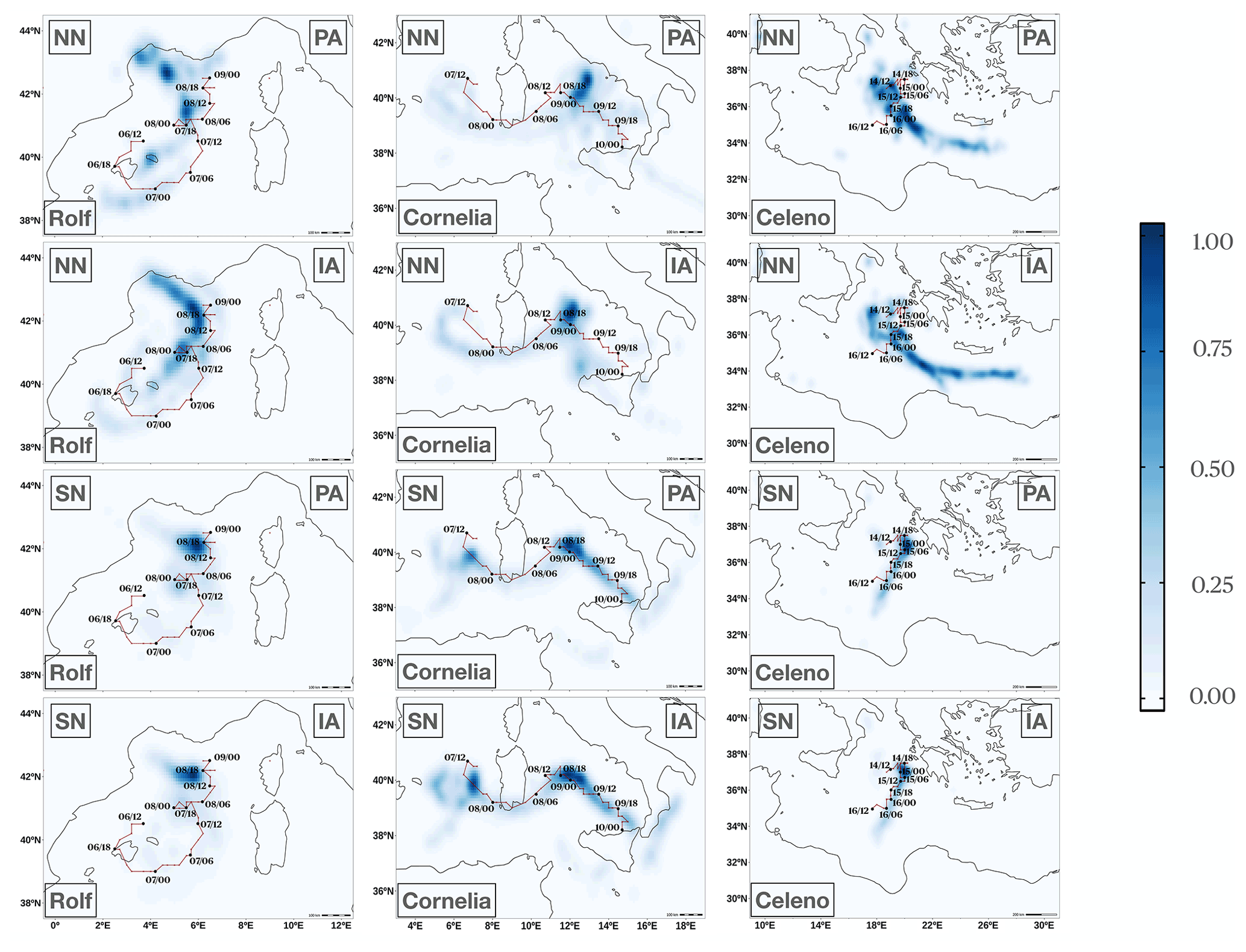
Figure 2 Normalized KDEs built on top of the medicane positions along the tracks belonging to the nudging-aerosol ensembles for medicanes Rolf (left), Cornelia (center) and Celeno (right). In red, the track of each medicane as a result of running the TITAM (Pravia-Sarabia et al., 2020a) tracking algorithm on ERA5 hourly reanalysis data is superimposed for the time steps in which a medicane is found by the algorithm. Labels (in day/hour format) and black points are placed every 6 h for the sake of clarity.

To offer a more comprehensive view of the results, Fig. 3 summarizes the main outcome for each member within the ensemble of simulations. Medicanes are separated in rings; and colors indicate, for the first two rows, the minimum SLP reached in each simulation for the four nudging-aerosol ensembles. The widths of the ring sector are proportional to the relative duration of the events (with respect to the maximum duration of a simulation inside the event simulation ensemble). The two bottom panels focus on the difference in depth of the storm when the interactive calculation of aerosols is considered and when it is not (reddish colors indicate deeper storms when IA is considered), the third row thus being the result of subtracting the first from the second row. For these two panels, widths of the outer rings are proportional to the length of the most compact set of points for the IA simulations and widths of the inner rings to that length for the PA ones. Differences between the left and right panels illustrate the impact of using spectral nudging (right) versus leaving simulations free (left). In line with what was concluded from previous figures, this Fig. 3 summarizes and highlights the fact that in NN simulations, IA produces deeper and longer-lasting medicanes as compared to those reproduced with PA. With respect to the initialization time, there seems to be a nearly random response to the initial conditions (variability in the azimuthal direction). The use of SN drastically – yet not completely – reduces these differences but leads to even longer-lived medicane structures (in which, for the cases of Cornelia and Celeno, the simulations approach the observed tracks), and reduces the variability introduced by the run-up time.

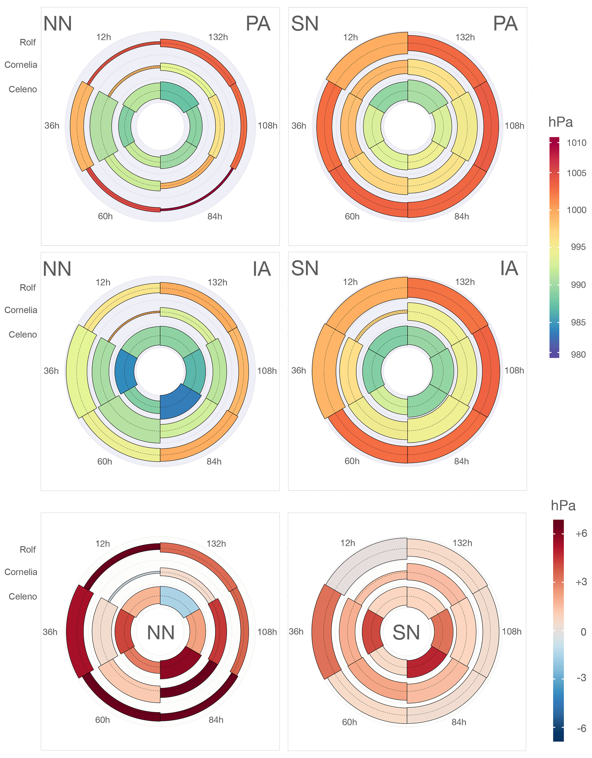
Figure 3 Medicanes are separated into rings across radial direction (inner Celeno, middle Cornelia, outer Rolf). The different run-up times are shown in six ring portions. In the first two rows, colors indicate the minimum SLP reached in each simulation for the four nudging-aerosol simulation ensembles; ring sector widths are proportional to the relative duration of the events. In the last row, the absolute difference (colors) in the minimum SLP among the medicane centers reached during the medicane's lifetime between the IA and PA simulations is shown for each medicane and run-up time. Thus, a red color represents a deeper SLP minimum of the medicane center's SLP values for the IA simulations, and the larger the asymmetry between the widths of the upper and lower halves of each portion of the rings, the higher the influence of using IA in the medicane duration. For each ring portion, the width of the outer half is proportional to the length of the compact set of points in the IA simulation and that of the inner part to the one in the PA simulation. A dashed line separates both. All ring widths are normalized with respect to the maximum duration among all the simulation ensembles for the medicane (24 simulations).

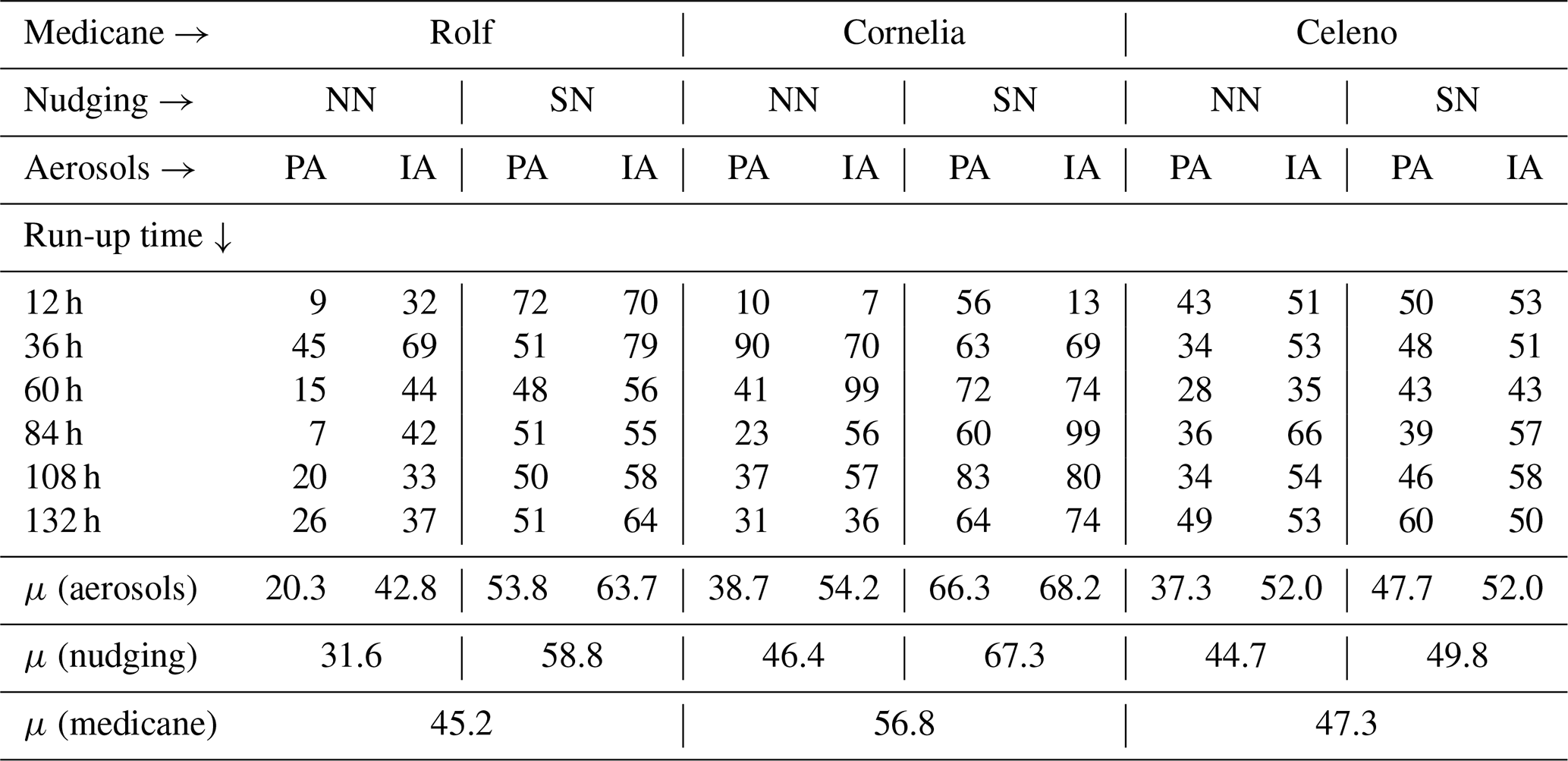
A more quantitative analysis is shown in Tables 1 and 2, containing both the minimum SLP reached by the medicane center and the duration of the medicane (length of the compact set of points) reproduced in each simulation, respectively. The μ quantity reduces the ensemble through the sample mean for each aggregated recursive level (aerosols – ensemble with the different run-up times; nudging – ensemble with the different run-up times and PA and IA configurations; medicane – ensemble with the different run-up times, PA and IA configurations, and NN/SN configurations).

Table 1 Summary of the minimum SLP reached by the medicanes in the 72 simulation ensembles. The μ quantity reduces the ensemble through the sample mean for each aggregated recursive level.

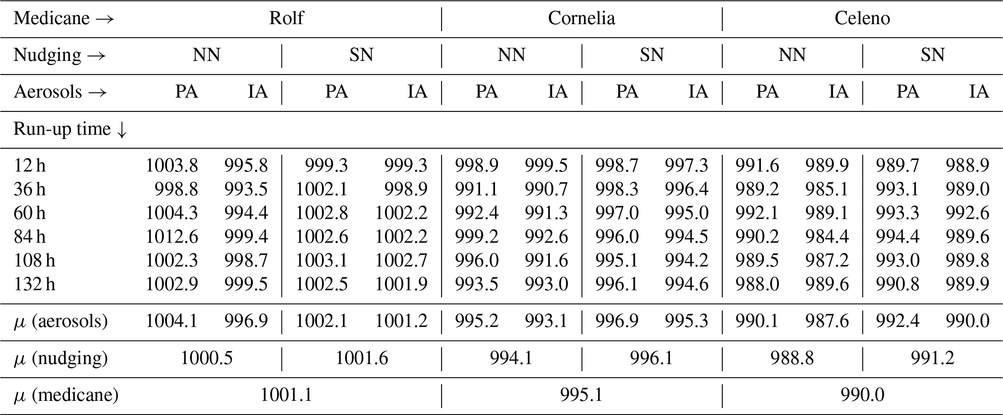
Table 2 Summary of the medicane duration – number of points in the compact set – of the 72 simulation ensembles. The μ quantity reduces the ensemble through the sample mean for each aggregated recursive level.

With respect to the spectral nudging effect, although long-lived medicane structures are generated for the SN configuration, they do not reach the intensity of those reproduced in the NN simulations. The explanation to this effect lies in the spectral nudging mechanism: forcing the meteorological fields to resemble the large-scale dynamics produces alterations in the nudged fields (temperature, humidity and wind) above the PBL. Henceforth, the temperature field does not freely evolve, and deep convection may be interrupted, thus limiting the intensification potential of the medicane. Figure 4 supports this statement, showing that the warm core is broken-off in the 500–800 hPa layer when SN is introduced. In Fig. 4, a set of height–radius cross sections of the equivalent potential temperature (θ_e) is produced by time-averaging the cross sections for the time steps in which a medicane is found for the NN (top) and SN (bottom) simulations of medicanes Rolf, Cornelia and Celeno, starting with 36 h of run-up time.

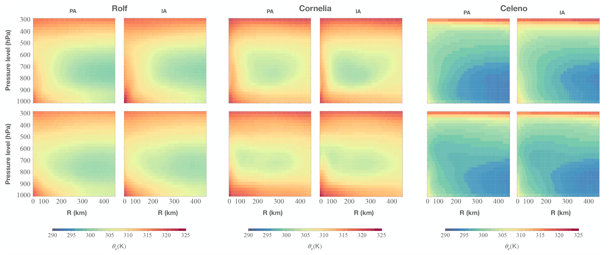
Figure 4 Time-averaged height–radius cross sections of the equivalent potential temperature (θ_e) over all time steps in which a medicane is found in the NN (top) and SN (bottom) simulations for medicanes Rolf (simulation starting 5 November 2011 at 00:00 UTC with 36 h of run-up time), Cornelia (simulation starting on 5 October 1996 at 00:00 UTC with 36 h of run-up time) and Celeno (simulation starting on 13 January 1995 at 00:00 UTC with 36 h of run-up time).

3.2 Proposed intensification mechanism: SSA–wind feedback

It has been previously discussed that IA calculation leads to deeper and longer medicane tracks. As introduced in Sect. 1, our main initial hypothesis, given the close nature of medicanes to tropical cyclones, is that the online calculation of SSA allows for the existence of a positive feedback with surface wind. Although this feedback is irrelevant for an early emergence of convective activity, generally fostered by a cold cut-off low in upper levels in the case of medicanes (Emanuel, 2005), it becomes essential once the core circulation is established. For the sake of examining the hypothesis of the existence of this feedback, we choose two NN simulations of Rolf starting on 5 November 2011 at 00:00 UTC because of (1) their closeness to the observed medicane track, (2) the low SLP they reach, and (3) the robust and stable structure they develop (not in intensity, but in terms of their track, it is the IA and PA pair in which the most similar storm is developed in both simulations). Figure 5 depicts the temporal evolution of the differences in equivalent potential temperature (θ_e) between the IA and PA simulations along the vertical of the medicane center.

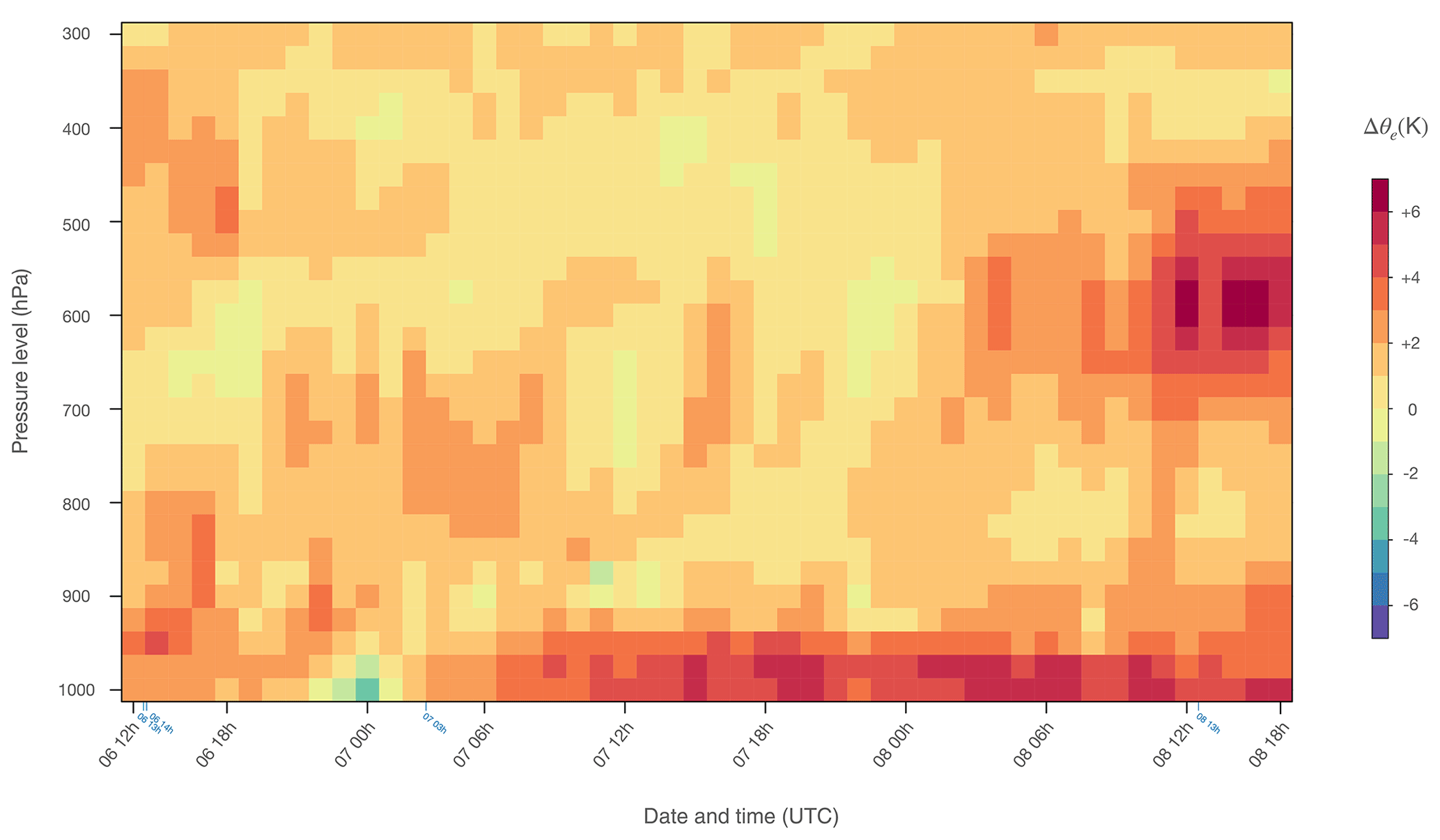
Figure 5 Difference in equivalent potential temperature between the IA and PA simulations for each output time step (horizontal axis) in which both the PA and IA simulations find a medicane for Rolf starting on 5 November 2011 at 00:00 UTC. Results are presented for each pressure level (vertical axis) in the vertical of the medicane center. Red colors indicate higher equivalent potential temperatures, and thus more available energy, for the IA simulation. Blue marks on the horizontal axis refer to the time steps in which the medicane structure is lost, and hence the tracking algorithm does not find a medicane center in any of the two compared cases. For these time steps, there is no vertical profile of temperature of the medicane core. The time axis labels (horizontal axis) are presented in day (DD) and hour (HH) format, all dates referring to November 2011.

In general, higher (orange to red colors) θ_e values are found for the IA case, meaning that more convective potential energy comes into play in the form of hot moist air in the low troposphere when aerosols are interactively solved at each time step of the model. This is specially evident for time steps after 7 November, when the medicane starts to gain strength, releasing more latent heat of condensation due to the stronger convection and thus producing more water vapor under higher surface wind conditions. Another related aspect, the warm core structure, is presented in Fig. 6 by means of the time-averaged height–radius cross sections of θ_e (top panels) along the latitudes of the medicane center, for both the PA (left) and IA (right) NN simulations of Rolf starting with 36 h of run-up time. Figure 6 clearly reveals that the core equivalent potential temperature is higher for the IA case, this being especially true for the lower tropospheric and surface levels given the strong presence of moist air in this layer. In the bottom panels of Fig. 6, the anomaly of potential temperature (θ^′) in time-averaged height–radius cross sections along the latitudes of the medicane center is presented for the same two simulations, showing a net heating of the storm core, the maximum in the 500–800 hPa layer, which seems to be related to core dynamics.

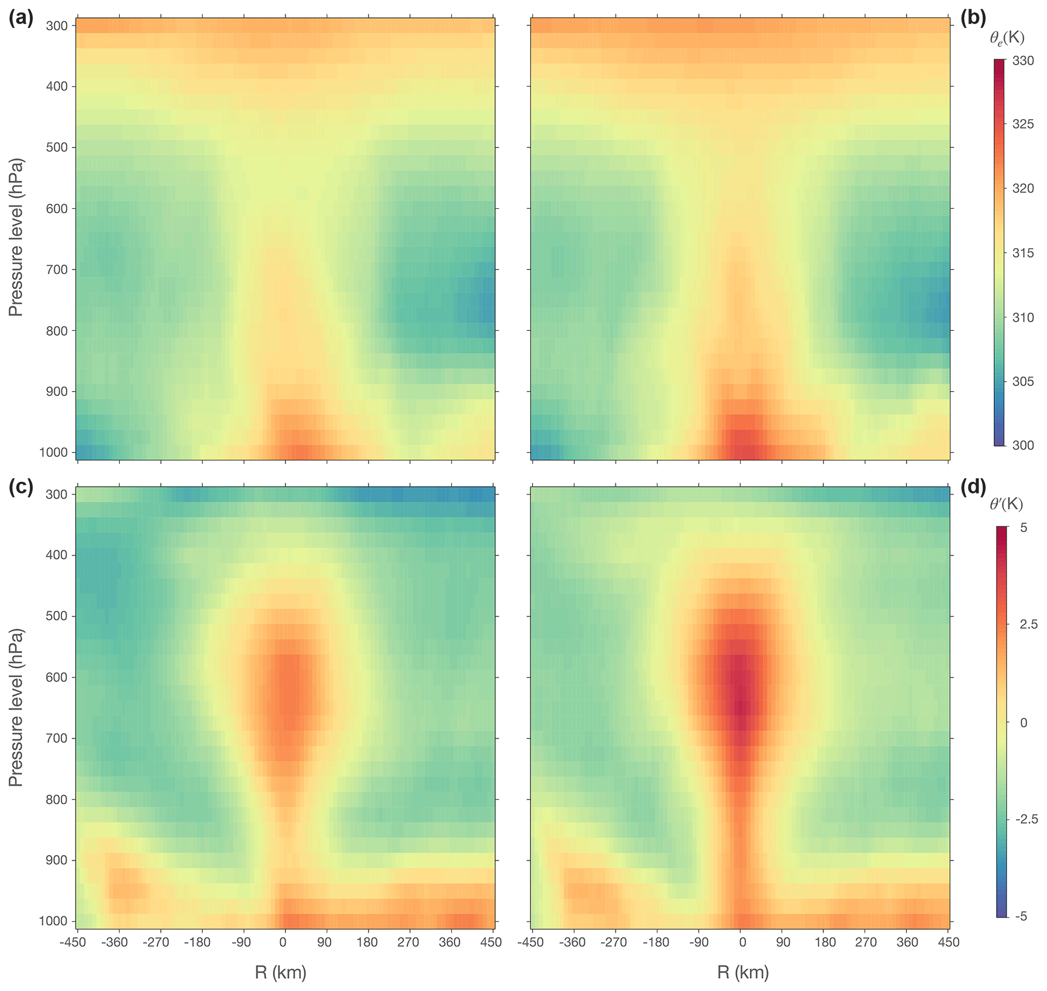
Figure 6 Time-averaged height–radius cross sections of the equivalent potential temperature (θ_e) (a, b) and the anomaly of potential temperature (θ^′) (c, d) along the medicane center latitudes for both the PA (a, c) and IA (b, d) NN simulations of Rolf starting with 36 h of run-up time. The anomaly of potential temperature is calculated for each level and with respect to the level time and spatially averaged potential temperature.

To fully understand the processes undergone by aerosols and clouds, the distribution of hydrometeors is examined, revealing the form in which the thermal energy is handled by the system. This is shown in Fig. 7, in which a time-averaged and azimuthally averaged height–radius cross section is presented along the medicane centers found for the simulations of Rolf starting on 5 November 2011 at 00:00 UTC (36 h of run-up time) with prescribed (left) and interactive (right) aerosol calculation; both simulations are run without spectral nudging. Figure 7 shows (from top to bottom) cloud water mixing ratio, rain water mixing ratio and droplet number mixing ratio for both the PA (left column) and IA (right column) simulations.

Figure 7 Time-averaged and azimuthally averaged height–radius cross sections of (a, b) cloud water mixing ratio (QCLOUD, kg kg⁻¹), (c, d) rain water mixing ratio (QRAIN, kg kg⁻¹) and (e,f) droplet number mixing ratio (QNDROP, kg⁻¹) for PA (a, c, e) and IA (b, d, f) simulations of Rolf starting with 36 h of run-up time (i.e., on 5 November 2011 at 00:00 UTC), both without spectral nudging. Distance from the medicane center is represented on the horizontal axis and atmospheric pressure levels on the vertical axis. The three scales must be multiplied by the factor preceding the units in the legend titles.

Figure 7 indicates that in the case in which the largest medicane deepening is found, although accompanied by a higher thermal energy, lower cloud droplet numbers and less cloud water content come into play, but more rain water is produced. Diving into the microphysics, a plausible explanation resides in the Köhler curves and mechanism of CCN activation as cloud droplets. Intense wind blowing over the ocean surface creates sea spray, which contains organic matter and inorganic salts that form SSA (Gong et al., 1997). SSAs are coarse particles quickly reaching the critical radius and being activated early as CCN at low supersaturation rates according to Köhler theory (Köhler, 1936), thus being highly prone to condensational growth (Jensen and Nugent, 2017). The existence of SSA enables an early, rapid and strong latent heat release in the lower troposphere which enhances deep convection, ultimately leading to an intensification of surface winds under low supersaturation conditions in the early medicane stage. Conversely, prescribed aerosol concentrations used in PA simulations lead to a high amount of fine particles with low hygroscopicity hardly activated as CCN and competing for water vapor uptake, thus producing a higher number of small droplets which are barely converted into raindrops.

4 Summary and conclusions

In this contribution, an ensemble of 72 simulations have been conducted to analyze the role of SSA feedbacks in the development and intensification of three different medicanes. Results show a clear dependence of both the track and intensity of the medicanes simulated on the calculation of interactive aerosols as their consideration leads to longer and deeper medicanes in the simulations. The proposed mechanism to explain this difference is that, in contrast to simulations with prescribed aerosols (as usually included in meteorological models), when interactive aerosols are introduced, the presence of coarse particles is taken into account, and the hygroscopic characteristics of SSA are considered, thus allowing the early attainment of critical radius and an enhancement of a strong latent heat release in the lower tropospheric levels. Conversely, when aerosols are prescribed and constant, finer particles are considered, and less activation of aerosols to CCN is produced, which lowers the velocity of condensational growth, leading to lower rates of latent heat production, and the suppression of warm rain provided the difficulty of small aerosols to grow to droplet size. Hence, the coupling of the meteorological model to an online chemistry module seems to be of paramount significance for the formation and evolution of a medicane. An interactive calculation of aerosols provides realistic SSA concentrations which, combined with the ability of the model to introduce hygroscopic and microphysical properties for the different species, favors the simulation of intense deep convection processes, which are crucial in this type of storm.

Initialization time largely modulates the output of the medicane simulations, thus being a source of great variability. Highly influenced by the initial conditions, these simulations are prone to lose the necessary conditions for a medicane to be triggered and maintained. Despite this sensitivity, there seems to be no privileged run-up time to simulate medicanes, and no systematic deviation is produced by this factor. Hence, modifying the initialization time is analogous to perturbing the initial conditions in a system highly sensitive to initial conditions. This result needs to be highlighted as the different run-up times can thus be regarded as an ensemble of perturbed initial conditions, and therefore the results obtained related to the importance of an interactive aerosol calculation are robust within this ensemble.

Spectral nudging leads to longer but less intense medicane tracks. Besides the fact that it seems useful for producing “realistic” medicanes in some cases, like that of Celeno, the storms do not seem to be fully developed when SN is introduced. Given the vertical character of medicane structures, any forcing introduced by synoptic-scale dynamics may provoke a misalignment in the medicane core or a break in the deep convective structure. Specifically, the asymmetric upper–lower tropospheric forcing derived from the spectral nudging technique without in-PBL influence causes the vertical alignment of the medicane core to deviate, introducing an artificial vertical shear that hampers the formation of deep convection. However, further analysis on the wavelength and in-PBL spectral nudging would be required to completely determine whether spectral nudging could be beneficial for medicane simulations. As for now, and despite our initial intuition related to the importance of binding the initial conditions, the results confirm that the spectral nudging seems not to be valid for individual case studies, its utility being limited to the downscaling of global climate models.

Finally, this contribution discusses the differences between simulations with and without SSA feedbacks, but no assessment is provided on whether differences imply a better agreement with actual medicanes. The main reason for this is the lack of reliable observations over the sea to carry out a comprehensive validation of the simulations. Therefore the contribution focuses on the physical mechanisms reproduced by the model and provides arguments supporting their feasibility. Given the great similarities of medicanes with tropical cyclones in their mature stage, it seems clear that the possibility for medicanes to produce their own SSA within a feedback process needs to be accounted for by the simulations. The analysis included here indeed shows that enabling this possibility leads to deeper and longer medicane tracks. Therefore the natural question emerging is to what extent this deepening of the storm is realistic. Although the lack of observations to carry out validations hampers such an assessment, including these processes can only lead to a more realistic simulation of medicanes. Models, and specifically their microphysics or the presence and effects of aerosols, are strongly parameterized. Even if an eventual validation could demonstrate that simulations without SSA feedback, i.e., shallower storms, are closer to observations, this would not mean that ignoring this feedback produces better results. Instead, it would demonstrate that the model is heavily tuned to produce better results when important feedback processes are ignored. An important factor to take into account is the change in the sea surface roughness on the wind stress due to the presence of spume droplets (Liu et al., 2012b; Kudryavtsev and Makin, 2011). It is believed that at very high wind speeds a deep part of the marine atmospheric surface layer is filled with spray droplets – spume – originating from intensively breaking waves which form the spray droplet suspension layer. Sea sprays generated by wave breaking and wind-tearing wave crests modify the wind profile and prevent the water surface from being dragged by the wind directly, which in turn reduces the drag coefficient and levels off the wind stress under highs winds (Liu et al., 2012a). Considering this effect may be important for a correct reproduction of sea spray production under high wind conditions (close to hurricane force, i.e., in the strongest medicanes), according to the results in Rizza et al. (2021) its omission may be consequential for the particular case study addressed in this work, and a coupling with an ocean model would be useful for a thorough inquiry into this question. However, according to the values provided in Liu et al. (2012a), the sea spray takes effect on the drag coefficient as the wind speed approaches the range of 25–33 m s⁻¹, which is hardly reached in the studied medicanes. On this basis, the validity of the results presented herein should not suffer alterations due to this effect of sea spray on ocean surface roughness, and the conclusions here included should be valid. Therefore, from the results included in this paper it becomes evident that the inclusion of SSA feedback is a fundamental mechanism in the development of tropical-like storms, and simulations aiming at studying these phenomena should not neglect its importance.