the Creative Commons Attribution 4.0 License.
the Creative Commons Attribution 4.0 License.
 | 23 Aug 2021
Comparative assessment of TROPOMI and OMI formaldehyde observations and validation against MAX-DOAS network column measurements
Isabelle De Smedt
Gaia Pinardi
Corinne Vigouroux
Steven Compernolle
Alkis Bais
Nuria Benavent
Folkert Boersma
Ka-Lok Chan
Sebastian Donner
Kai-Uwe Eichmann
Pascal Hedelt
François Hendrick
Hitoshi Irie
Vinod Kumar
Jean-Christopher Lambert
Bavo Langerock
Christophe Lerot
Cheng Liu
Diego Loyola
Ankie Piters
Andreas Richter
Claudia Rivera Cárdenas
Fabian Romahn
Robert George Ryan
Vinayak Sinha
Nicolas Theys
Jonas Vlietinck
Thomas Wagner
Ting Wang
Huan Yu
Michel Van Roozendael
The TROPOspheric Monitoring Instrument (TROPOMI), launched in October 2017 on board the Sentinel-5 Precursor (S5P) satellite, monitors the composition of the Earth's atmosphere at an unprecedented horizontal resolution as fine as 3.5 × 5.5 km2. This paper assesses the performances of the TROPOMI formaldehyde (HCHO) operational product compared to its predecessor, the OMI (Ozone Monitoring Instrument) HCHO QA4ECV product, at different spatial and temporal scales. The parallel development of the two algorithms favoured the consistency of the products, which facilitates the production of long-term combined time series. The main difference between the two satellite products is related to the use of different cloud algorithms, leading to a positive bias of OMI compared to TROPOMI of up to 30 % in tropical regions. We show that after switching off the explicit correction for cloud effects, the two datasets come into an excellent agreement. For medium to large HCHO vertical columns (larger than 5 × 10¹⁵ molec. cm−2) the median bias between OMI and TROPOMI HCHO columns is not larger than 10 % (< 0.4 × 10¹⁵ molec. cm−2). For lower columns, OMI observations present a remaining positive bias of about 20 % (< 0.8 × 10¹⁵ molec. cm−2) compared to TROPOMI in midlatitude regions. Here, we also use a global network of 18 MAX-DOAS (multi-axis differential optical absorption spectroscopy) instruments to validate both satellite sensors for a large range of HCHO columns. This work complements the study by Vigouroux et al. (2020), where a global FTIR (Fourier transform infrared) network is used to validate the TROPOMI HCHO operational product. Consistent with the FTIR validation study, we find that for elevated HCHO columns, TROPOMI data are systematically low (−25 % for HCHO columns larger than 8 × 10¹⁵ molec. cm−2), while no significant bias is found for medium-range column values. We further show that OMI and TROPOMI data present equivalent biases for large HCHO levels. However, TROPOMI significantly improves the precision of the HCHO observations at short temporal scales and for low HCHO columns. We show that compared to OMI, the precision of the TROPOMI HCHO columns is improved by 25 % for individual pixels and by up to a factor of 3 when considering daily averages in 20 km radius circles. The validation precision obtained with daily TROPOMI observations is comparable to the one obtained with monthly OMI observations. To illustrate the improved performances of TROPOMI in capturing weak HCHO signals, we present clear detection of HCHO column enhancements related to shipping emissions in the Indian Ocean. This is achieved by averaging data over a much shorter period (3 months) than required with previous sensors (5 years) and opens new perspectives to study shipping emissions of VOCs (volatile organic compounds) and related atmospheric chemical interactions.
- Article
(34638 KB) - Full-text XML
-
Supplement
(1655 KB) - BibTeX
- EndNote


Satellite observations of tropospheric formaldehyde (HCHO) columns have been used for years to support air quality and chemistry–climate-related studies from the regional to the global scale. Formaldehyde is an intermediate gas in almost all oxidation chains of non-methane volatile organic compounds (NMVOCs), leading to the production of carbon monoxide (CO) and eventually carbon dioxide (CO2). NMVOCs are, together with nitrogen oxides (NOx), CO and methane (CH4), among the most important precursors of tropospheric ozone. NMVOCs also produce secondary organic aerosols and influence the concentrations of hydroxyl radical (OH), the main tropospheric oxidant. The major HCHO source in the remote atmosphere is CH4 oxidation. Over the continents, the oxidation of other NMVOCs emitted from vegetation, fires, traffic and industrial sources results in important and localized enhancements of the HCHO levels. Because of its short lifetime (of the order of a few hours), HCHO in the boundary layer can be related to the release of a large number of short-lived volatile hydrocarbons. Furthermore, HCHO observations provide information on the chemical oxidation processes in the atmosphere, including CO chemical production from CH4 and NMVOCs, the oxidation of isoprene into HCHO, which allows the quantification of midday OH (Wells et al., 2020), and the tropospheric ozone production regimes that depend on the HCHO to NO2 ratios (Jin et al., 2020).
Satellite observations of formaldehyde columns in the troposphere have been extensively reported in the literature from a number of nadir UV sensors, e.g. the Global Ozone Monitoring Experiment (GOME; Chance et al., 2000; Palmer et al., 2001; De Smedt et al., 2008), SCanning Imaging Absorption spectroMeter for Atmospheric CHartographY (SCIAMACHY; Wittrock et al., 2006; De Smedt et al., 2008, 2010), Ozone Monitoring Instrument (OMI; González Abad et al., 2015; De Smedt et al., 2015, 2018; Kaiser et al., 2018; Levelt et al., 2018), Global Ozone Monitoring Experiment-2 (GOME-2; De Smedt et al., 2012, 2015; Vrekoussis et al., 2010; Hewson et al., 2013; Hassinen et al., 2016) and Ozone Mapping and Profiler Suite (OMPS; Li et al., 2015; González Abad et al., 2016). They are used in many studies related to air quality and climate change (e.g. Stavrakou et al., 2014, 2015, 2016, 2018; Fortems-Cheiney et al., 2012; Marais et al., 2012; Mahajan et al., 2015; Choi and Souri, 2015; Zhu et al., 2016; Chan Miller et al., 2017; Jin et al., 2017; Barkley et al., 2017; Cao et al., 2018; Khan et al., 2018; Surl et al., 2018; Shen et al., 2019; Su et al., 2019; Zyrichidou et al., 2019; Jin et al., 2020; Souri et al., 2020; Wells et al., 2020; Franco et al., 2021; Opacka et al., 2021).
Launched on board of the European Copernicus Sentinel-5 Precursor (S5P) satellite on 13 October 2017, the TROPOspheric Monitoring Instrument (TROPOMI, Veefkind et al., 2012) is designed for the daily monitoring of the troposphere at the global scale. Compared to its predecessor OMI, its spatial resolution is about 16 times better with at least the same signal-to-noise ratio per ground pixel. The improved TROPOMI capabilities for the observation of HCHO have been illustrated for the detection of fire plumes and their transport (Alvarado et al., 2020; Theys et al., 2020) and the detection of rapid changes in anthropogenic emissions related to the COVID crisis in China and India (Levelt et al., 2021; Sun et al., 2021). The TROPOMI observations extend the historical time series of midday observations performed using OMI. Both datasets are used in combination for long-term trend studies (Li et al., 2020). It is therefore important to evaluate their level of agreement and to report on the best practices to combine datasets from different sensors.
The TROPOMI vertical column product requirements specify a single-measurement precision of 12 × 1015 molec. cm−2, 4 × 10¹⁵ molec. cm−2 at 20 km spatial resolution and a systematic uncertainty lower than 40 %–80 % (ESA, 2021). The Copernicus user requirements, primarily defined for NMVOC measurements, are more stringent. For the environmental air quality theme, the required maximum uncertainty is defined as 60 % or 1.3 × 10¹⁵ molec. cm−2 (least stringent), at the spatial resolution of 20 km and with a revisit time of 2 h. The space and time resolutions are less stringent for the climate theme (30 % or 1.3 × 10¹⁵ molec. cm−2, 50 km, 3 d) (Bovensmann et al., 2011; Langen et al., 2017).
Given these rather strict product requirements and the diversity of the NMVOC species, lifetimes and sources (biogenic, biomass burning or anthropogenic), a validation approach addressing a large variety of conditions worldwide (tropical, temperate and boreal forests, urban and sub-urban areas) is needed as are continuous measurements in order to obtain good statistics and capture the seasonal variations. Vigouroux et al. (2020) validated the operational TROPOMI HCHO product using a global network of Fourier transform infrared (FTIR) instruments. The study concluded that overall the HCHO product fulfils the requirements of the TROPOMI mission. Compared to the FTIR data, the TROPOMI HCHO columns present a negative bias over high concentrations sites (−31 % for HCHO columns larger than 8 × 10¹⁵ molec. cm−2) and a positive bias for clean sites (+26 % for HCHO columns lower than 2.5 × 10¹⁵ molec. cm−2). Based on clean sites, an upper limit of 1.3 × 10¹⁵ molec. cm−2 was estimated for the deviation of daily observations at a spatial resolution of 20 km. It was also pointed out that this level of random uncertainty, although reaching the Copernicus user requirements, is about twice as large as the expected theoretical noise (individual pixel precision divided by the square root of the number of observations). However, Vigouroux et al. (2020) do not address the consistency of TROPOMI HCHO with other satellite products and MAX-DOAS (multi-axis differential optical absorption spectroscopy) HCHO observations.
The present paper is a follow-up of De Smedt et al. (2018), where the HCHO retrieval algorithm applied to both OMI and TROPOMI sensors was presented. Here we concentrate on a global study of 3 years of HCHO observations with TROPOMI, and we analyse their consistency with OMI data. Throughout the paper, we discuss the improved capabilities of TROPOMI for the detection of HCHO at different temporal and spatial scales, from background conditions to high emissions. We start with a few illustrations of the TROPOMI capabilities for HCHO monitoring from space (Sect. 3). We then provide a detailed comparison with the OMI QA4ECV HCHO dataset (Sect. 4). In Sect. 5, a global network of MAX-DOAS instruments is used to validate the OMI and TROPOMI HCHO datasets. Finally, in Sect. 6, we illustrate the enhanced capability of TROPOMI for the detection of very small HCHO emissions with the identification of a signal over shipping lanes in the Indian Ocean.
2.1 OMI instrument and QA4ECV HCHO product
The Aura satellite was launched in July 2004, in a low-Earth polar orbit crossing the Equator at 13:30 LT. On board Aura, the Ozone Monitoring Instrument (OMI) is a nadir-viewing imaging spectrometer that measures the solar radiation backscattered by the Earth's atmosphere and surface over the wavelength range from 270 to 500 nm (Levelt et al., 2006). Operational Level 2 (L2) products include vertical columns of O3, SO2, NO2, HCHO, BrO and OClO as well as cloud and aerosol information. OMI has a 2600 km wide swath (divided into 60 across-track positions or rows), providing near-daily global coverage. However, due to a detector row anomaly that occurred after a few years of operation, an increasing number of rows had to be filtered out leading to gradual degradation of the coverage. The OMI ground pixel size varies from 13×24 km2 at nadir to 28×150 km2 at the edges of the swath.
The OMI QA4ECV HCHO product was developed by a European consortium (BIRA, IUP, MPIC, KNMI, WUR) (De Smedt et al., 2017, https://doi.org/10.18758/71021031) in the framework of the EU-FP7 QA4ECV project. A detailed step-by-step study was performed for HCHO and NO2 retrievals as part of a community effort to homogenize GOME, SCIAMACHY, GOME-2 and OMI, leading to state-of-the art European products (http://www.qa4ecv.eu, last access: 18 August 2021). For this study, we use the version 1.2 of the OMI HCHO dataset that now spans 15 years (2005–2020; Boersma et al., 2018; Lorente et al., 2017; Nightingale et al., 2018; Zara et al., 2018). Note that within QA4ECV, a homogenized dataset of NO2 and HCHO MAX-DOAS reference measurements (QA4ECV_MAXDOAS, https://uv-vis.aeronomie.be/groundbased/QA4ECV_MAXDOAS/index.php, last access: 18 August 2021) was also developed for satellite validation (see Sects. 2.4 and 5).
2.2 TROPOMI instrument and the HCHO operational product
On board the S5P platform, which – like Aura – flies in a low-Earth afternoon polar orbit with a local overpass time of 13:30 LT, the TROPOMI instrument is based on an imaging spectrometer measuring in the ultraviolet (UV), visible (VIS), near-infrared (NIR) and shortwave infrared (SWIR) spectral regions (Veefkind et al., 2012). Operational L2 products include vertical columns of O3, SO2, NO2, HCHO, CO and CH4 as well as cloud and aerosol information. TROPOMI has a 2600 km wide swath (divided into 450 across-track positions or rows), providing near-daily global coverage. The spatial resolution at nadir, originally of 3.5 × 7 km2 (across-track × along-track) has been refined to 3.5 × 5.5 km2 on 6 August 2019, by a change in the along-track integration time. The size of the pixels remains more or less constant towards the edges of the swath (the largest pixels are ∼ 14 km wide) (L1b ATBD, https://sentinel.esa.int/documents/247904/2476257/Sentinel-5P-TROPOMI-Level-1B-ATBD, last access: 18 August 2021; L1b readme file, http://www.tropomi.eu/sites/default/files/files/publicSentinel-5P-Level-1b-Product-Readme-File.pdf, last access: 18 August 2021).
The retrieval algorithm of the TROPOMI HCHO L2 product is directly inherited from the QA4ECV OMI algorithm with the aim to create a consistent time series of early afternoon observations. For this study, we use a modified version of the TROPOMI level-2 HCHO operational data product, which starts in April 2018 (phase E2, reprocessed (RPRO) + Offline (OFFL), product versions 1.1.[5–8] + 2.1.3, https://doi.org/10.5270/S5P-tjlxfd2). Product versions are described in the Product Readme File (http://www.tropomi.eu/sites/default/files/files/publicSentinel-5P-Formaldehyde-Readme.pdf, last access: 18 August 2021).
2.3 HCHO retrieval algorithm for OMI and TROPOMI
The HCHO retrieval algorithm was fully described in De Smedt et al. (2018), and the successive adaptations of the algorithm are reported in the S5P product ATBD. Here we only provide a short description of the algorithm, which is based on a three-step DOAS method. First, the fit of the slant columns (Ns) is performed in the UV part of the spectra, in the fitting interval 328.5–359 nm. The HCHO cross section is from Meller and Moortgat (2000). All cross sections have been pre-convolved for every row separately with an instrumental slit function adjusted after TROPOMI launch. For the OMI product, the slit function of each row is adjusted daily and the cross sections are reconvolved accordingly. The DOAS reference spectrum is updated daily with an average of Earth radiances measured in the equatorial Pacific region from the previous day. The fit therefore results in a differential slant column, corresponding to the HCHO excess over sources compared to the remote background. In a second step, the conversion from slant to tropospheric vertical columns (Nv) is performed using a look up table of vertically resolved air mass factors (M) calculated at 340 nm with the radiative transfer model VLIDORT v2.6 (Spurr, 2008). Entries for each ground pixel are the observation geometry, the surface elevation and reflectivity, and clouds treated as reflecting surfaces and a priori tropospheric HCHO profiles. The surface albedo is taken from the monthly OMI albedo climatology at the spatial resolution of 1∘ × 1∘ (minimum Lambertian equivalent reflectivity, LER, Kleipool et al., 2008). A priori vertical profiles are provided by the TM5-MP daily analysis, at the spatial resolution of 1∘ × 1∘ (Williams et al., 2017). A cloud correction based on the independent pixel approximation (Boersma et al., 2004) is applied for cloud fractions (CFs) larger than 0.1. Finally, to correct for any remaining global offset and possible stripes arising between the rows, a background correction is performed based on the HCHO slant columns in the Pacific Ocean (Ns,0). For the TROPOMI operational product, Ns,0 is based on the 4 previous days. For this study, and for the OMI product, we perform the correction on the current day in order to further reduce the stripes. To compensate for a background HCHO level in the equatorial Pacific (due to the methane oxidation), a vertical column of HCHO () is taken from the TM5 model in the reference region. The resulting tropospheric HCHO vertical column can be written as follows:
with M0 the air mass factor in the reference sector. Intermediate quantities and auxiliary data are all stored in the L2 files (see the product user manual for TROPOMI and OMI). Several diagnostic variables are provided together with the measurements. The column averaging kernels and the a priori profiles are given for each observation. The tropospheric column uncertainty is resolved into its random (precision) and systematic components (accuracy) and is provided for every individual pixel.
The main difference between the OMI and TROPOMI algorithms lies in the cloud product that is used to compute air mass factors. While the QA4ECV OMI product is based on the O2–O2 absorption feature around 477 nm and considers a fixed cloud albedo of 0.8 (version 2.0, Veefkind et al., 2016), the TROPOMI product uses the S5P operational cloud product in CRB (Cloud as Reflecting Boundary) mode (OCRA/ROCINN-CRB; Loyola et al., 2018). The S5P ROCINN algorithm is based on the O2 A band around 760 nm and simultaneously retrieves cloud height and cloud albedo. Systematic differences between the cloud parameters will result in differences in the air mass factors, influencing the comparisons. To mitigate the impact of this difference between OMI and TROPOMI, we also switch off the cloud correction by replacing the cloud-corrected air mass factor (AMF) by an equivalent clear-sky AMF (Mclear, no cloud correction applied) also provided in the L2 product. Based on Eq. (1), the following simple transformation can be applied:
Note that this transformation has an effect on observations with cloud fractions comprised between 0.1 and 0.4. Indeed, no cloud correction is applied for CF < 0.1 and observations with CF > 0.4 are filtered out from the analysis.
2.4 MAX-DOAS datasets
MAX-DOAS instruments retrieve the abundance of atmospheric trace species in the lowermost troposphere (Hönninger et al., 2004; Wagner et al., 2004; Wittrock et al., 2004; Heckel et al., 2005). Based on DOAS analyses (Platt and Stutz, 2008) of the scattered sky light under different viewing elevations, high sensitivity close to the surface is obtained for the smallest elevation angles, whereas measurements at higher elevations provide information on the rest of the column. MAX-DOAS measurements have been used in several studies to validate satellite HCHO columns (Vigouroux et al., 2009; Franco et al., 2015; De Smedt et al., 2015; Chan et al., 2019, 2020; Ryan et al., 2020; Kumar et al., 2020). However, a global network of MAX-DOAS instruments has not been used yet for the validation of HCHO columns from space.
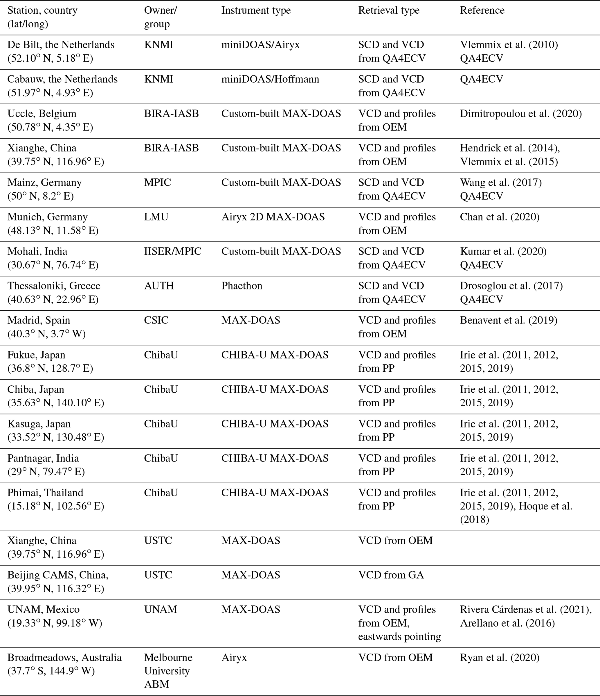
Ground-based data used in this study are presented in Table 1. Apart from the QA4ECV MAX-DOAS dataset, which relies on harmonized HCHO retrievals (Pinardi et al., 2013; QA4ECV D3.8, http://www.qa4ecv.eu/sites/default/files/QA4ECV_D3.8_v1.0_web.pdf and D3.9, http://www.qa4ecv.eu/sites/default/files/D3.9.pdf, http://www.qa4ecv.eu/node/9#overlay-context=, last access: 18 August 2021), the MAX-DOAS data sets used here were generated by instrument principal investigators using non-harmonized settings. The conversion to vertical columns and/or vertical profiles relies on methods of various complexity levels. Table 1 includes details about the retrieval strategy adopted by the different teams. These include the following:
-
GA: geometrical approximation; the vertical column is determined using a single-scattering approximation adequate for moderately high-elevation angles α (typically 30∘) so that a simple geometrical air mass factor (AMF ≡ SCDVCD = ; SCD stands for slant column density, and VCD stands for vertical column density) (Hönninger et al., 2004; Brinksma et al., 2008; Ma et al., 2013) can be used;
-
QA4ECV: the vertical column is calculated using tropospheric AMFs based on climatological profiles and aerosol loads as developed during the QA4ECV project (QA4ECV_MAXDOAS_readmefile, http://uv-vis.aeronomie.be/groundbased/QA4ECV_MAXDOAS/QA4ECV_MAXDOAS_readme_website.pdf, last access: 18 August 2021); these data are less sensitive to relative azimuth angle than the purely geometric approximation presented above;
-
OEM: vertical profile algorithms using an optimal estimation method (Rodgers, 2000); these make use of a priori vertical profiles and associated uncertainties (Frieß et al., 2006; Clémer et al., 2010; Hendrick et al., 2014; Gielen et al., 2017; Wang et al., 2019a; Friedrich et al., 2019; Bösch et al., 2018);
-
PP: vertical profile algorithms based on parameterized profile shape functions; these make use of analytical expressions to represent the trace gas profile using a limited number of parameters (Irie et al., 2008, 2011; Li et al., 2010; Vlemmix et al., 2010; Wagner et al., 2011; Beirle et al., 2019).
Both OEM and parameterized profiling approaches provide vertical profiles of aerosols and HCHO with good sensitivity in the 0–4 km altitude range, in which one to three independent pieces of information in the vertical dimension are available (Vlemmix et al., 2015; Frieß et al., 2016, 2019). Recent intercomparison studies (Vlemmix et al., 2015; Frieß et al., 2019; Tirpitz et al., 2021) show that both OEM and parameterized inversion approaches lead to consistent results in terms of tropospheric vertical columns but to larger differences in terms of profiles. The accuracy of the MAX-DOAS technique depends on the SCD retrieval noise, the uncertainty of the HCHO absorption cross sections, the choice of the a priori profile shape and the uncertainty of the tropospheric AMF calculation. MAX-DOAS HCHO slant columns from several instruments have been compared during international large-scale campaigns (CINDI-1 and 2, e.g. Pinardi et al., 2013; Kreher et al., 2020) showing relatively large median differences and larger noise compared to other slant column product comparisons (e.g. NO2). For HCHO, the slant column precision depends strongly on the signal-to-noise performance of the DOAS instrument with significantly better results for low-noise research-grade MAX-DOAS instruments (Pinardi et al., 2013; Kreher et al., 2020). The estimated total uncertainty on HCHO VCD is of the order of 30 % to 60 % in polluted conditions. This includes both random (∼ 5 % to 30 % depending on instrumental signal-to-noise ratio) and systematic (20 %) slant column contributions (Pinardi et al., 2013).
Table 1MAX-DOAS HCHO datasets included in the validation exercise. GA stands for geometrical approximation, OEM for optimal estimation method and PP for parameterized profiling.
2.5 Data use and method
For this study, unless specified otherwise, we filter the satellite data based on the quality assurance values (QA) (Product Readme File, http://www.tropomi.eu/sites/default/files/files/publicSentinel-5P-Formaldehyde-Readme.pdf). QA > 0.5 filters out most observations presenting an error flag or a solar zenith angle larger than 70∘, a cloud radiance fraction (CRF) at 340 nm larger than 0.6, an air mass factor smaller than 0.1, surface reflectivity larger than 0.2 or an activated snow/ice flag. It should be noted that, in the first versions of the operational product, the QA values were not correctly assigned over snow/ice regions, above 75∘ of SZA (solar zenith angle) and sometimes over cloudy scenes. This issue has been corrected from version 2.1.3 (July 2020). For this study, we therefore reassigned QA values using the above-mentioned filters.
We calculated daily gridded data at a resolution of 0.05∘ × 0.05∘ in latitude and longitude, both for OMI and TROPOMI, using the Harp atmospheric toolbox (https://atmospherictoolbox.org/harp/, last access: 18 August 2021). Throughout the paper, daily and monthly averages are obtained from daily grids. For each day, we require the region to be filled with a least 50 % of valid grid cells, with a minimum of 10 TROPOMI observations (two OMI observations).
For the satellite–satellite and the satellite–ground-based comparisons, we calculate the median of the absolute differences (absolute bias) and the median of the relative differences (relative bias) in each region or station (relative either to TROPOMI in the case of satellite–satellite or to the MAX-DOAS columns in the case of satellite–ground-based). The corresponding median absolute-value deviations (MADs) of the absolute and relative differences are a robust estimate of the combined observation and comparison variability. The MAD is defined as the median of the absolute-value deviations from the data's median:
where the factor k=1.4826 is used to ensure a correspondence with the 1σ standard deviation for normal distribution. The bias is regarded as statistically significant if it exceeds , where N is the number of collocated pairs (days or months). We also derive correlation, slope and offset of the linear regression using the robust Theil–Sen estimator (Sen, 1968) as done in Vigouroux et al. (2020).
As an illustration of the data product, Fig. 1 displays the global seasonal distribution of tropospheric HCHO columns derived from TROPOMI observations between March 2018 and February 2021. The overall seasonality of the HCHO columns is largely driven by the emissions of NMVOCs from the vegetation and by the interannual variability of surface temperatures and solar radiation. As can be seen, in the south-eastern US for example, the seasonal amplitude is very important and dominated by biogenic emissions during summertime. On top of biogenic emissions, wildfires present a large variability. Since 2018, many fire events have occurred worldwide and can be traced, e.g., in HCHO columns during summer 2018 and 2020 in the western US or during summer 2019 in Siberia. After a decrease of about 10 years (De Smedt et al., 2015), South America experienced two intense fire seasons in 2019 and 2020. The year 2020 was also marked by the huge Australian and Californian wildfires, respectively, in January and October 2020, detectable in the seasonal maps. In comparison to biogenic and pyrogenic emissions of natural origin, the contribution due to anthropogenic NMVOC emissions to the total HCHO columns is generally lower. Although their oxidation is also enhanced by sunlight, anthropogenic emissions show less seasonality than natural emissions, and their detection is therefore generally easier in annual maps. This is illustrated in Fig. 2, which presents 3-year averages of HCHO columns over Asia, the Arabic Peninsula, the US, and Central and South America, providing detailed information about the spatial distribution of HCHO at the regional and urban scale. Europe and Africa are shown in the Supplement (Fig. S1 in the Supplement). Note that the colour scale has been adapted to the regions. Large urban areas are clearly visible in the HCHO distribution in Asia, the Middle East and South America. With a lower magnitude, US cities are also clearly detectable, such as Houston, Dallas or Los Angeles. HCHO levels are noticeably lower in Europe, but some urban areas are visible in the southern countries.
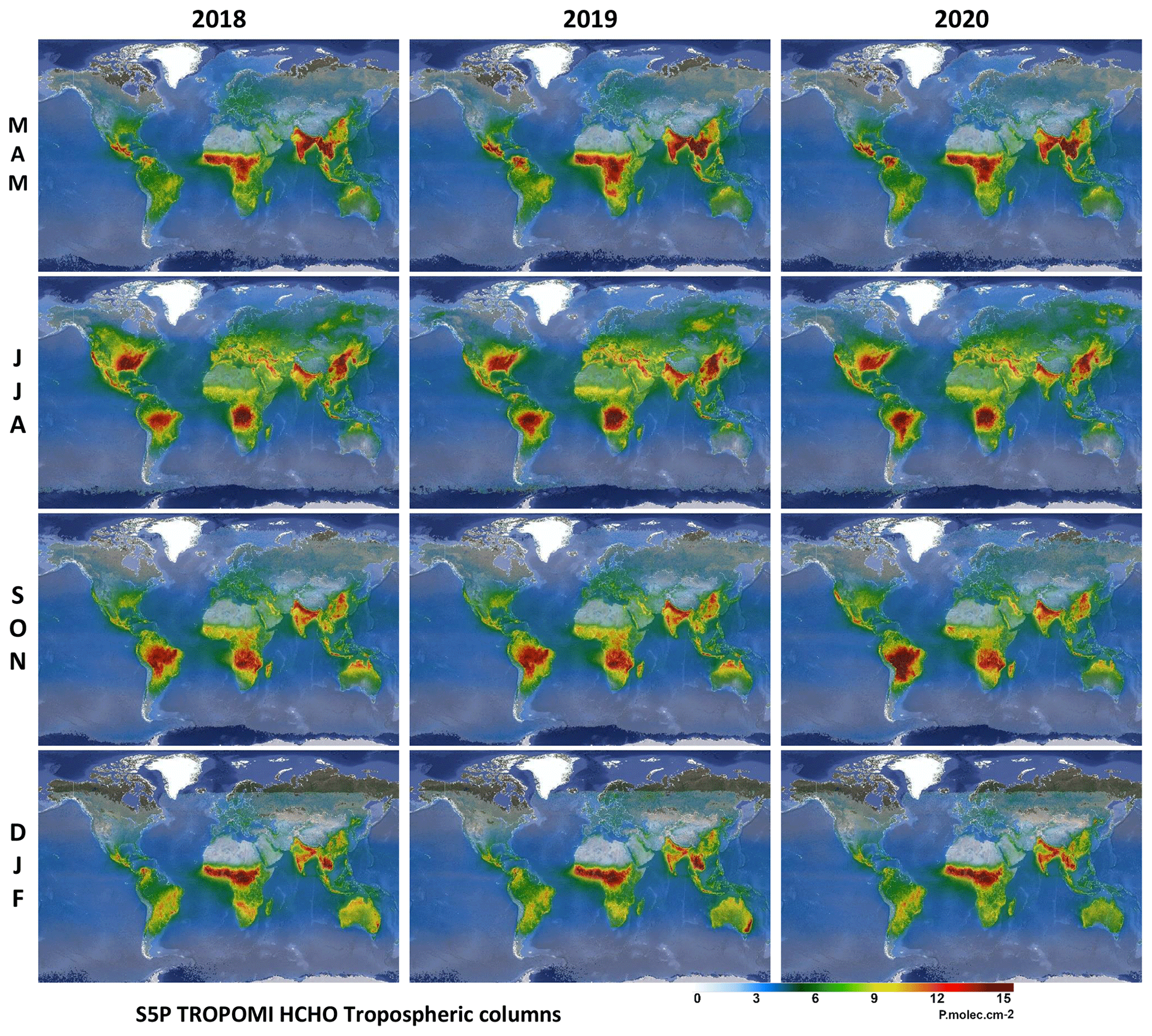
Figure 1Seasonal maps of TROPOMI HCHO tropospheric columns during the first 3 years of measurements (March 2018–February 2021), on a spatial grid of 0.05∘ in latitude and longitude. Observations are filtered using the qa_values > 0.5 (max scale: 15 × 1015 molec. cm−2). Modified Copernicus Sentinel-5P satellite data, OFFL L2 HCHO product, BIRA-IASB/DLR/ESA/EU.
The quality of the TROPOMI observations also allows observing HCHO columns on a much shorter timescale with an unprecedented definition. Daily observations of fire plumes are a clear step forward in the satellite remote sensing of HCHO. They can be observed over much longer distances than before, thanks to the daily global coverage, coupled with the finer spatial resolution and the improved signal-to-noise ratio, allowing the detection of lower columns transported further away (Alvarado et al., 2020; Theys et al., 2020). It is not only wildfires but also important anthropogenic emission plumes that can be observed on a daily basis, for example on the eastern coast of Saudi Arabia. A few illustrations are given in Fig. S2. The TROPOMI performances for the observations of HCHO are discussed more quantitatively throughout the paper in terms of precision and bias as a function of the HCHO levels and of the temporal and spatial scales.

Figure 2Multi-annual regional maps of TROPOMI HCHO tropospheric columns (March 2018–February 2021), on a spatial grid of 0.05∘ in latitude and longitude. Observations are filtered using the qa_values > 0.5. Modified Copernicus Sentinel-5P satellite data, OFFL L2 HCHO product, BIRA-IASB/DLR/ESA/EU.
In this section, we evaluate the consistency between OMI and TROPOMI HCHO tropospheric columns. In addition, we present the gain in precision obtained with TROPOMI. The analysis relies on 32 months of simultaneous measurements from April 2018 to December 2020, allowing for a meaningful comparison at different scales. We first compare the precision obtained on individual measurements and then proceed with a comparison of the precisions achieved when averaging data at different spatial and temporal scales.
4.1 HCHO slant column precision
The random uncertainty of the tropospheric HCHO column is dominated by the error on the fitted slant column densities (SCDEs), which is directly related to the signal-to-noise ratio (SNR) of the measurement. From this point of view, TROPOMI performs significantly better than previously launched nadir UV–VIS satellite instruments. In the spectral range of HCHO retrievals (328.5–359 nm), the SNR of the TROPOMI spectra exceeds pre-flight requirements that were based on OMI specifications (Kleipool et al., 2018; Ludewig et al., 2020).
Figure 3 presents global maps of SCDE averaged over 3 months during summer 2019, from OMI and TROPOMI. From the improved SNR of TROPOMI in the UV range, TROPOMI HCHO SCDEs of individual observations are about 25 % lower than OMI ones. Over remote areas, the TROPOMI SCDE is about 6 × 10¹⁵ molec. cm−2, while it is 8 × 10¹⁵ molec. cm−2 for OMI. Slant column density errors are also improved over emission areas and at larger SZAs. Contrary to OMI, the effect of the South Atlantic Anomaly is absent in TROPOMI SCDE. This probably results from a better shielding of the instrument against extra-terrestrial high-energy radiation. The implemented iterative spike algorithm (De Smedt et al., 2018) is also more efficient because of the lower noise level of the instrument. Note however that over mountains, TROPOMI SCDEs are higher than OMI ones. The most obvious effect is observed over the Himalayas, but other chains such as the Andes or the Rocky mountains are also affected. This effect has been identified as a scene inhomogeneity effect (Richter et al., 2018, 2020). The effect is also visible along the borders of bright lakes or white surfaces. OMI retrievals are also affected by scene inhomogeneity effects, but the larger size of the ground pixels and the larger mean SCDE values make its detection more difficult. We note that in the 3-year averaged maps of the HCHO tropospheric columns, some collocated artefacts appear (Fig. 2, e.g. the white sands in the US, Tuz Golu lake in Turkey or Lake Mackay in Australia). Most of the snow/ice scenes are eliminated by the quality assurance values. The observations could however be better filtered over mountains and along the lake borders or even corrected during the fit of the slant columns as demonstrated for NO2 and glyoxal (Lerot et al., 2021). The relatively coarse albedo climatology also needs to be updated with a TROPOMI-based product, better defined in space and time (Loyola et al., 2020).
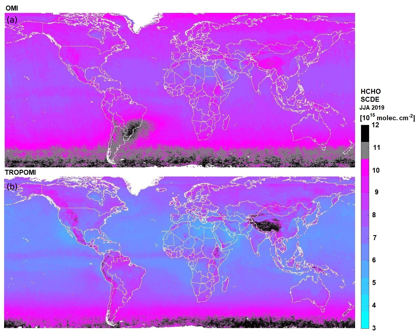
Figure 3Average HCHO slant column density fitting error (SCDE) retrieved from OMI (a) and TROPOMI (b) in JJA 2019, on a spatial grid of 0.05∘ in latitude and longitude.
The OMI SCDEs have been very stable over the years, showing a limited increase of about 5 % between 2005 and 2019 (De Smedt et al., 2018). However, the number of valid OMI observations has decreased by about 30 % during the same period (−50 % at large SZA) due to the row anomaly. In order to evaluate the stability of the TROPOMI HCHO retrievals during the first 3 years, Fig. 4 presents the time series of the TROPOMI HCHO slant column errors in the remote Pacific Ocean as a function of latitude and instrumental rows. As expected, we observe an increase in the noise for large SZAs and for the 25 first and last rows of the scan, which have a different detector binning (L1b ATBD, https://sentinel.esa.int/documents/247904/2476257/Sentinel-5P-TROPOMI-Level-1B-ATBD). The fact that the algorithm makes use of daily updated radiances as reference for the DOAS fit allows for very stable results in time and across the rows. Only the change in pixel size in August 2019 (L1b readme file, http://www.tropomi.eu/sites/default/files/files/publicSentinel-5P-Level-1b-Product-Readme-File.pdf) resulted in a moderate step increase in the SCDE of about 15 %. These values are compared to the observed standard deviation of the slant columns in the same regions (see Fig. S3). We observe a very good agreement between the SCDEs and the standard deviation, indicating that they give a good representation of the random errors.
The reported uncertainty in the tropospheric vertical columns due to random errors corresponds to the SCDE divided by the AMF for each observation. In the equatorial Pacific, the TROPOMI vertical column precision is about 5 × 10¹⁵ molec. cm−2, while it is 7 × 10¹⁵ molec. cm−2 for OMI. It is larger over continental emissions, where the AMFs are generally smaller than 1.

Figure 4TROPOMI HCHO slant column density errors (SCDEs) as a function of the latitude (a) or the detector row (b). The step increase on 6 August 2019 reflects the change in the TROPOMI pixel size (indicated with the black line).
4.2 HCHO tropospheric columns
Figure 5 presents the yearly averaged OMI and TROPOMI HCHO vertical columns (Nv_clear) for 2019. Even at this level of averaging, the lower noise level of TROPOMI is very clear, especially for low to medium HCHO levels. We observe an overall good agreement of the columns both in magnitude and in their spatial distribution. Differences in TROPOMI and OMI yearly averages range from +2 × 10¹⁵ molec. cm−2 over the tropics to −2 × 10¹⁵ molec. cm−2 over midlatitude regions. Differences tend to increase with latitudes. However, as the quality of the TROPOMI observations is improved at large solar zenith angles, more data in winter months are kept in the TROPOMI dataset, which can influence yearly averaged columns at those latitudes. In order to provide quantitative comparisons, we calculated daily and monthly averaged columns in 35 regions covering a broad range of emission levels and observation conditions (large black boxes in Fig. 5). As the regions are large, many observations are included (on average 500 per day for OMI, 12 500 per day for TROPOMI). To obtain daily and monthly comparison pairs, we keep coincident days of observations and follow the methodology presented in Sect. 2.5.
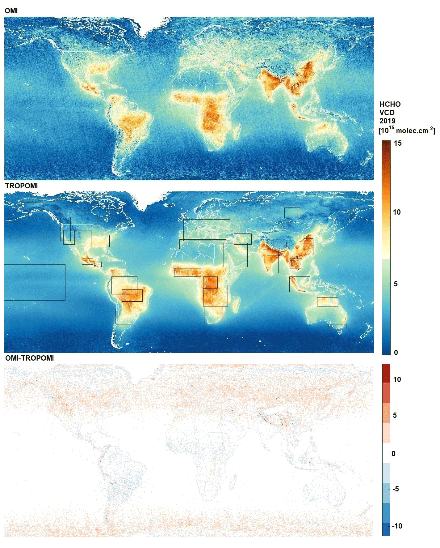
Figure 5Average HCHO tropospheric column (Nv_clear) retrieved from OMI (first line) and TROPOMI (second line) in 2019. Limits of the regions selected for the comparisons are shown on the TROPOMI map. Differences between OMI and TROPOMI maps are shown on the last panel. The same grid is used for both datasets (0.05∘). Data are filtered using the product quality flags. The large black boxes on the TROPOMI maps represent the regions used in the comparisons (see Figs. 6 and 7).
An example of a time series over equatorial Africa is presented in the first panel of Fig. 6, where monthly averaged Nv_clear is shown, and comparison numbers are provided in the figure. In the equatorial African region, the seasonal cycle is marked by two peaks during the dry seasons and two minima during the wet seasons. In 2019, the minimum was particularly low, observed in both the OMI and TROPOMI time series, while the maxima tend to increase over the years. More examples of time series can be found in Fig. S4. In all the regions, the seasonal and interannual variability of the HCHO columns are observed very consistently with OMI and TROPOMI.
Figure 7 presents the absolute and relative biases between OMI and TROPOMI HCHO tropospheric columns for all regions. Numbers are provided for daily averaged columns applying a cloud correction (Nv) or not (Nv_clear). Regions are sorted as a function of the averaged TROPOMI HCHO column. At this large spatial scale, the regions over equatorial Africa, northern China and northern India present the largest annual columns worldwide, with median levels larger than 10 × 1015 molec. cm−2. Tropical regions in South America, Africa and Asia present elevated levels of HCHO as well, with annual averaged columns larger than 8 × 10¹⁵ molec. cm−2.
Looking at Nv comparisons, it appears that the OMI HCHO columns present a positive bias compared to TROPOMI from 17 ± 2.5 % for the columns larger than 5 × 10¹⁵ molec. cm−2, to 30 ± 5 % for the lower columns. This bias exceeds 50 % in northern latitudes (> 45∘) and low-emission (< 2 × 10¹⁵ molec. cm−2) regions of Canada and Alaska. However, when comparing Nv_clear, the biases are strongly reduced below 10 % in all regions where the HCHO levels are larger than 5 × 10¹⁵ molec. cm−2, and the TROPOMI columns are found to be slightly larger than OMI on average ( %). In northern midlatitudes/moderate-emission (2–5 × 10¹⁵ molec. cm−2) regions such as Europe, central and western US, north-western Canada, Siberia, or Tibet, OMI columns present a remaining bias of about 15 ± 3 %, while in the regions of Canada and Alaska, a larger bias of about +30 ± 7 % remains. Note that we observe biases lower than 10 % in the Maghreb and southern Australia regions, despite their relatively low columns or low latitudes.
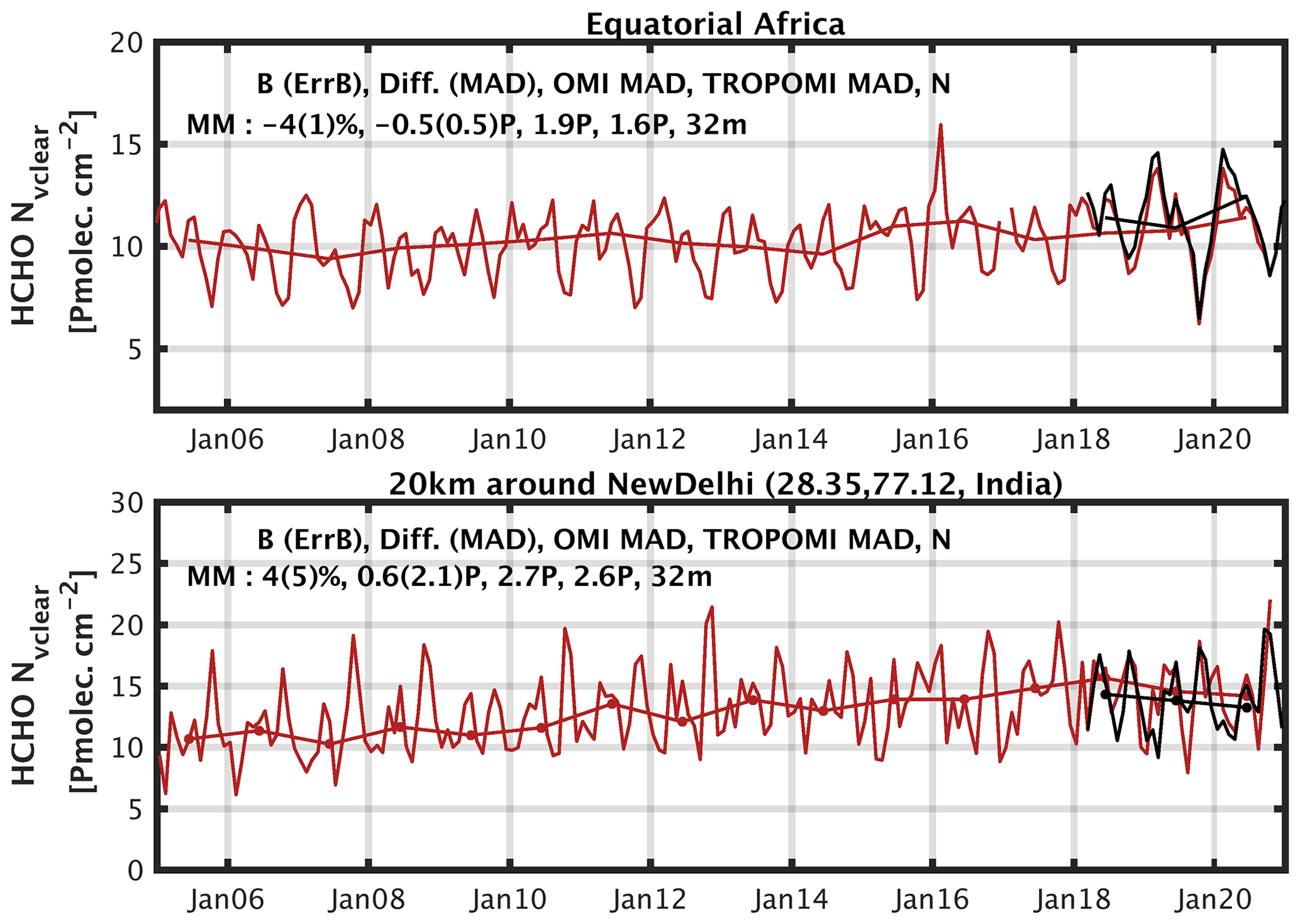
Figure 6Examples of monthly and yearly averaged HCHO columns (Nv_clear) retrieved from OMI (October 2004–December 2020, in red) and TROPOMI (2018–December 2020, in black) at two different spatial scales selected for the comparison: a large region of equatorial Africa and a circle of 20 km radius over New Delhi in India. Absolute and relative biases between OMI and TROPOMI HCHO monthly averaged columns are given at the top of each panel as are the median deviations of the OMI and TROPOMI averaged columns. (Pmolec. cm−2 = 1 × 10¹⁵ molec. cm−2]).
We conclude that biases up to 30 % related to the cloud correction are observed over tropical regions where the clouds are the highest in altitude (Africa, South America, South Asia), and a smaller but systematic effect, up to 15 %, is observed over midlatitude polluted regions such as China, India, the US or Europe. We also note that the differences between Nv and Nv_clear are mainly significant for the OMI HCHO columns. It has been reported that the cloud pressures retrieved from TROPOMI and from OMI present a bias (OMI clouds are higher in altitude, Compernolle et al., 2021). This translates into OMI cloud-corrected air mass factors generally smaller than TROPOMI AMFs by 5 % to 30 %, depending on the cloud altitude, and therefore in a positive bias of the OMI HCHO VCD compared to the TROPOMI product. It is therefore important to keep in mind that the use of different cloud products may introduce inconsistencies, which may be resolved by using clear HCHO VCDs (Nv_clear).
Figure 8 shows the linear regression between OMI and TROPOMI monthly averaged columns, considering all regions together. The relation between OMI and TROPOMI is provided for Nv and Nv_clear. This shows that switching off the cloud correction in the OMI and TROPOMI HCHO products allows to significantly improve not only the slope (from 0.87 to 0.92) and the intercept (from 1.52 to 0.48 × 10¹⁵ molec. cm−2), but also the data scatter, i.e. the Pearson R correlation (from 0.74 to 0.98). When considering large-scale comparisons, the agreement between OMI and TROPOMI Nv_clear is therefore very satisfactory.
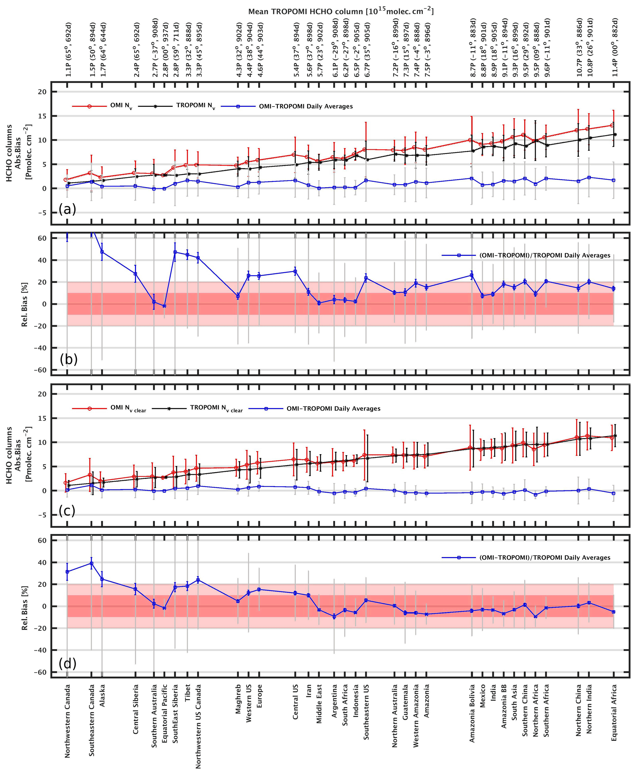
Figure 7Absolute and relative biases between OMI and TROPOMI HCHO daily averaged tropospheric columns using cloud-corrected AMF (Nv, a, b) or clear-sky AMF (Nv_clear, c, d) for the large regions represented on Fig. 5. Regions are sorted as a function of the median TROPOMI HCHO column. Values of the averaged HCHO columns are provided on the top axis as are the numbers of common days taken for the comparison and the latitude of the region. The median OMI (red) and TROPOMI (black) columns are plotted together with the absolute differences (in blue). Error bars represent the median deviations of the columns or the median absolute deviations of the differences (MAD, in grey). Statistical ErrB is also plotted for the relative bias (in blue). Pink areas indicate 10 % and 20 % bias. (Pmolec. cm−2 = 1 × 10¹⁵ molec. cm−2.)

Figure 8Scatter plots of OMI versus TROPOMI columns for the monthly means of collocated data. Results are shown for Nv (a) and Nv_clear (b). The correlation, slope and intercept of a linear regression using the robust Theil–Sen estimator are given in each panel and plotted as a blue line. The black dotted line is the 1 : 1 line. The colour indicates the latitude of the region. (Pmolec. cm−2 = 1 × 10¹⁵ molec. cm−2.)
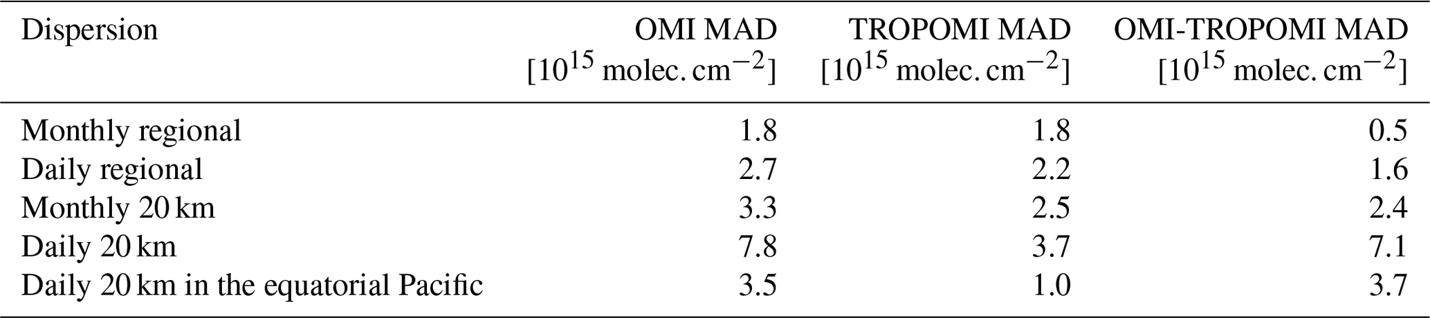
When averaging data over large regions, the dispersion due to random uncertainties is greatly reduced compared to individual observations. As summarized in Table 2, the median absolute deviations of the monthly averaged columns are equivalent for OMI and TROPOMI (1.8 × 10¹⁵ molec. cm−2), while the MADs of their differences are significantly lower (0.5 × 10¹⁵ molec. cm−2). This indicates that at this spatiotemporal resolution, the natural variability dominates the dispersion of the averaged observations. Looking at the daily averaged columns, the TROPOMI median deviation is lower than for OMI (2.2/2.7) but still larger than the MAD of their differences (1.5).
The improved spatial resolution of TROPOMI should allow for a better detection of localized HCHO columns. To address this question, we performed the same comparisons as for the large regions but looking at smaller areas of 20 km radius around cities. Figure 9 presents the absolute and relative biases of the monthly averaged HCHO columns (Nv_clear) for a large number of cities. At this spatial scale, Jakarta is the location with the largest median HCHO level (> 18 × 1015 molec. cm−2 over the 2018–2020 period). Indian, Chinese and other Asian cities follow as well as Mexico, Monterrey or Kinshasa (> 12 × 1015 molec. cm−2). Sao Paulo, Tehran and Cairo also present noticeably elevated HCHO levels (> 9 × 10¹⁵ molec. cm−2). An example over New Delhi is presented in the second panel of Fig. 6 and more examples can be found in Fig. S5.
When comparing OMI and TROPOMI Nv_clear around the cities, the same general behaviour as in the large regions can be observed. OMI presents a positive bias (20 ± 15 %) compared to TROPOMI for low to medium HCHO levels, while for medium to high levels, the agreement is very good on average (−1 ± 10 %). There are nevertheless a few exceptions where TROPOMI HCHO columns are significantly larger than the OMI ones. This is the case at La Réunion, Paramaribo, Nairobi, Bujumbura, Sao Paulo, Monterrey, Mexico or Jakarta. Those cities are located along marine coasts or lakes, at higher altitude, or are surrounded by mountains. In those cases, the finer spatial resolution of TROPOMI clearly improves the detection of the HCHO signal. For most other locations, however, the impact of the improved spatial resolution of TROPOMI on the HCHO columns is not detectable in the column magnitudes, when compared to OMI observations. This is likely related to the nature of the HCHO production that mostly is secondary from the oxidation of NMVOCs with various lifetimes (Stavrakou et al., 2015; Bauwens et al., 2016). Except for regions where the topography presents sharp discontinuities, this causes a natural spread of the HCHO columns at a scale larger than the TROPOMI spatial resolution.
Note however that at this spatial resolution (20 km radius), the level of noise is larger than for the regional averages and the TROPOMI-averaged columns are significantly more stable than the OMI ones, as evidenced by their median deviations (see Table 2). On a daily basis, the OMI columns present a dispersion of 7.8 × 10¹⁵ molec. cm−2, while the TROPOMI dispersion is about twice smaller (3.7 × 10¹⁵ molec. cm−2). In this case, the MAD of the differences (7.1 × 10¹⁵ molec. cm−2) is dominated by the noise in OMI observations. Note that these estimates still include the natural variability of the columns themselves. If an area of 20 km radius in the remote equatorial Pacific is considered, the observations represent constant background values and the seasonal variability is further reduced. In such conditions, the dispersion of the OMI daily observations is 3.5 × 10¹⁵ molec. cm−2 but only 1 × 10¹⁵ molec. cm−2 for TROPOMI. We show in the next section that validation with ground-based measurements brings further information on the satellite column precision.
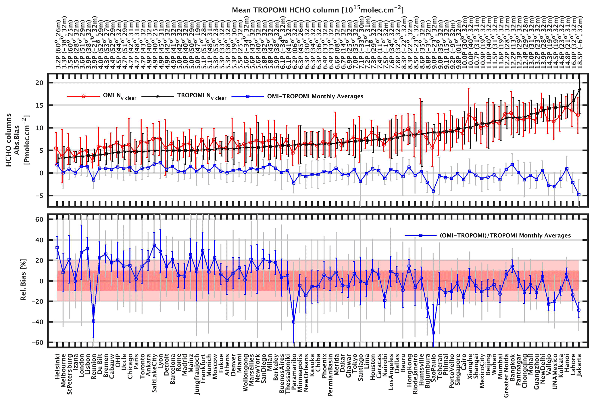
Figure 9Absolute and relative biases between OMI and TROPOMI HCHO monthly averaged tropospheric columns using clear-sky AMF (Nv_clear) within 20 km radius circles around selected cities, sorted as a function of the median TROPOMI HCHO column. Values of the averaged HCHO columns are provided on the top axis as are the numbers of months taken for the comparison and the latitude of the region. The median OMI (red) and TROPOMI (black) columns are plotted together with the absolute differences (in blue). Error bars represent the median absolute deviations (MADs) of the columns and of the differences (in grey). Statistical ErrB is also plotted for the relative bias (in blue). Pink areas indicate 10 % and 20 % bias. (Pmolec. cm−2 = 1 × 10¹⁵ molec. cm−2.)
Table 2Median absolute deviation of the OMI and TROPOMI daily and monthly averaged columns (Nv_clear), in large regions and in a 20 km radius area. MADs of differences between OMI and TROPOMI columns are also given in the last column.
Here, we present a validation exercise based on a network of 18 ground-based MAX-DOAS instruments. This effort complements the study of Vigouroux et al. (2020), which relied on a network of FTIR instruments. Compared to the FTIR instruments, the MAX-DOAS instruments provide a higher sensitivity in the boundary layer, where the bulk of HCHO is located. The MAX-DOAS network covers stations where the level of HCHO is significant, from medium to very large HCHO columns, while the FTIR network includes a larger number of remote stations. In this study, we validate in parallel the OMI and TROPOMI datasets. We first focus on a direct comparison of the satellite and MAX-DOAS tropospheric columns. The effect of the vertical smoothing is investigated in the next subsection for three stations.
5.1 Direct comparisons of tropospheric columns
For each station in Table 1, we consider daily averages of the satellite columns in a radius of 20 km around the instruments. We average MAX-DOAS columns between 11:00 and 16:00 local time. We keep coincident days of observations (OMI/MAX-DOAS, TROPOMI/MAX-DOAS) to obtain daily and monthly comparison pairs. Note that the time periods used for the comparison are not the same for OMI and TROPOMI and vary between the stations. To obtain the validation results, we follow the methodology presented in Vigouroux et al. (2020) (see Sect. 2.5).
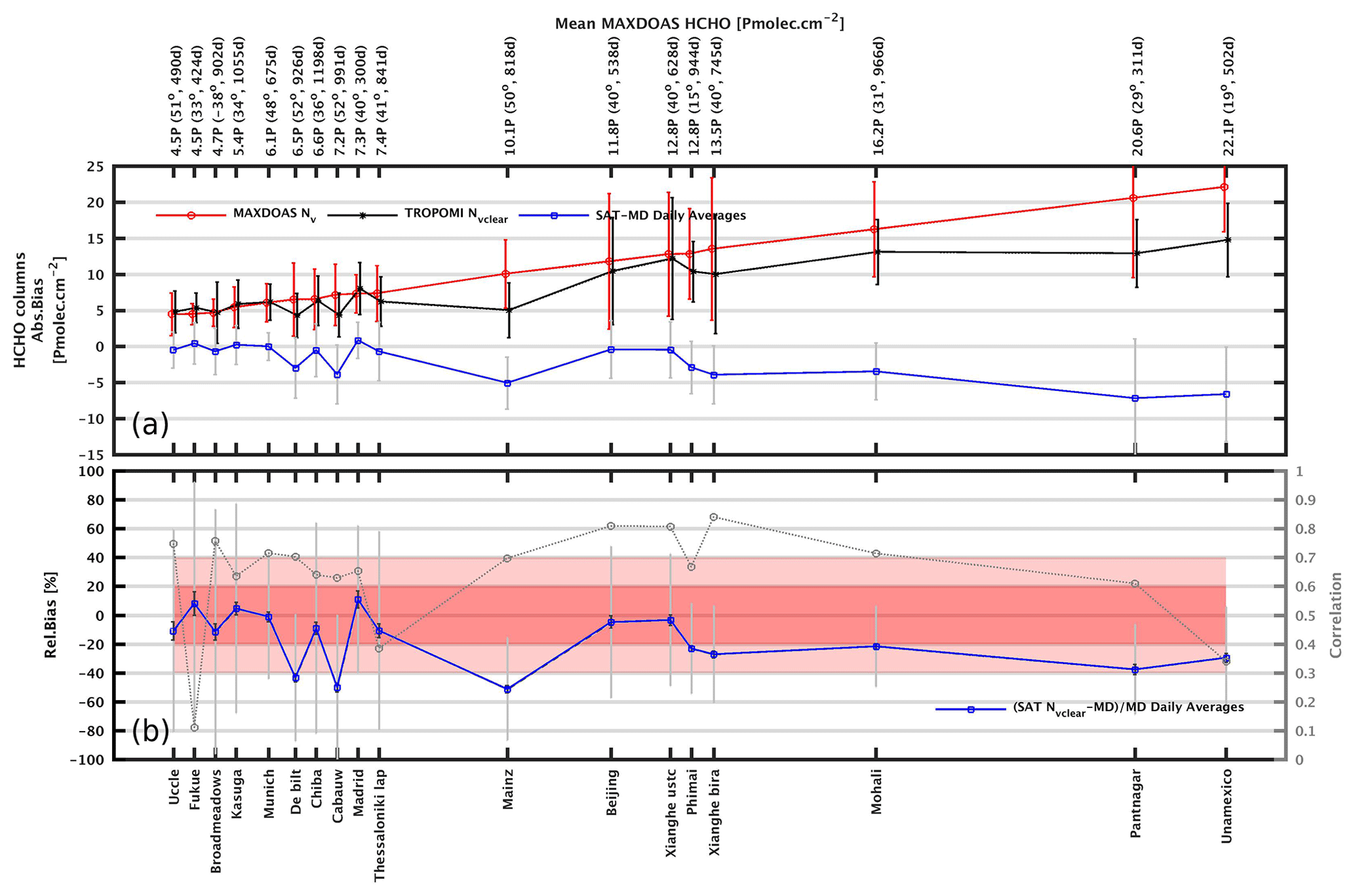
Figure 10Absolute (a, blue line) and relative biases (b) between MAX-DOAS and TROPOMI HCHO daily averaged tropospheric columns in a circle of 20 km radius around the stations. Regions are sorted as a function of the median MAX-DOAS HCHO column. In (a), the median MAX-DOAS (red) and TROPOMI (black) columns are plotted together with the differences. Error bars (in grey) represent the median absolute deviations (MADs) of the columns and of the differences. Statistical ErrB is also plotted for the relative bias (in blue). Pink areas indicate 20 % and 40 % bias. The correlation between the daily observations is given in (b) (grey circles). (Pmolec. cm−2 = 1 × 10¹⁵ molec. cm-2.)
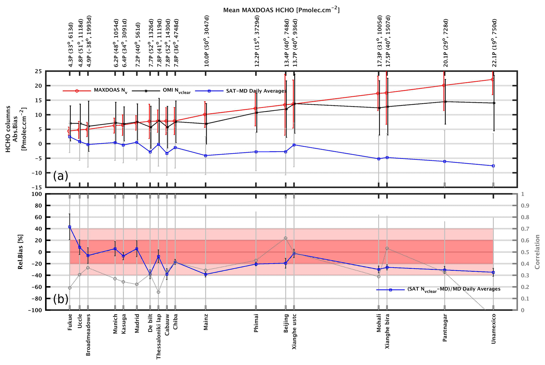
Figures 10 and 11 present the absolute and relative biases of the daily averaged columns as a function of the median MAX-DOAS HCHO column, respectively, for TROPOMI and OMI. A more detailed description for each station and for individual time series is presented afterwards. The values of the biases are similar for OMI and TROPOMI, except for the lowest columns in Uccle and Fukue, where OMI presents larger positive biases exceeding +20 %. In agreement with Vigouroux et al. (2020), TROPOMI columns do not present a significant bias for the range of HCHO levels from 4 to 8 × 10¹⁵ molec. cm−2. Note that, in contrast to FTIR data, the range of values covered by our MAX-DOAS network does not extend to columns lower than 4 × 10¹⁵ molec. cm−2. We observe that the stations in De Bilt and Cabauw tend to show somewhat stronger negative biases even for medium levels of HCHO, which might point to a network inhomogeneity. For larger HCHO columns (> 8 × 10¹⁵ molec. cm−2) and in agreement with the FTIR results, we observe that negative biases tend to increase for large HCHO columns such that the underestimation of the satellite columns reaches about −40 % for the largest columns. On the upper plot, the error bars represent the median absolute deviations of the columns and of their differences. It appears clearly that the MADs obtained with TROPOMI are substantially lower than those obtained with OMI. Note that the type of MAX-DOAS instrument (in particular its signal-to-noise ratio) may also influence the observed MAD at the different stations.
Figures 12, 13 and 14 present more detailed results for the stations in Europe, in Japan and Australia, and in China, India, Thailand and in Mexico, respectively. In each plot, the time series of the MAX-DOAS, OMI and TROPOMI data are displayed together. Results of the daily statistical analysis are given in each panel. At European stations, which show medium-range HCHO levels, we obtain contrasting results. With a mean HCHO column of 4.5 × 10¹⁵ molec. cm−2, Uccle is one of the stations with the lowest columns of the network presented in this paper. While OMI values show a positive bias (13 ± 15 %) and a poor correlation (0.3) with the MAX-DOAS, TROPOMI appears to be biased low ( %) but much better correlated (0.82) with the MAX-DOAS data. As opposed to Uccle, the observed biases in De Bilt, Cabauw and Mainz are largely negative (from −40 % to −50 %). The correlations found with TROPOMI are nevertheless much better than with OMI. Note that the median MAX-DOAS HCHO value in Mainz is larger than 10 × 1015 molec. cm−2, which is quite high for a European site. The results in Munich have been presented in detail in Chan et al. (2020). They are closer to what is found in Uccle, with a small positive bias for TROPOMI (1±3 %) and for OMI (6±13 %). Similarly in Madrid, OMI and TROPOMI results are very consistent with a mean bias of, respectively, 8±16 % and 10±6 %. In Thessaloniki, the negative bias is %, but the correlation is poorer than in Madrid.

Figure 12Time series of MAX-DOAS HCHO columns (blue), OMI Nv_clear (red) and TROPOMI Nv_clear (black) at European sites. Thick lines show monthly median values, and dots represent daily median values. Mean relative bias, median absolute deviations and correlations between the time series are provided for the daily averaged data. (Pmolec. cm−2 = 1015 molec. cm−2.)
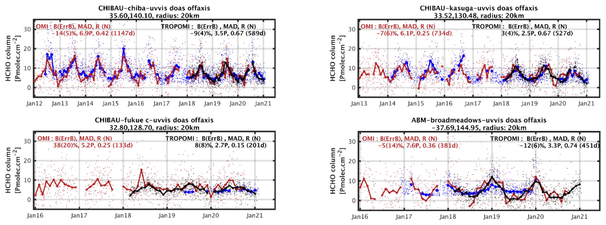
In Fig. 13, we show three Japanese stations operated by the CHIBA University. Mean HCHO levels in Japan are comparable to values found at European sites. In Chiba and Kasuga, TROPOMI and MAX-DOAS columns are strongly correlated (about 0.7), but on the island of Fukue the correlation is poor due to a lack of variability at this site. At all these sites, TROPOMI shows small biases relative to MAX-DOAS data ( % in Chiba, 3±4 % in Kasuga, 8±8 % in Fukue). The HCHO observations in Broadmeadows, in northern Melbourne, have been published by Ryan et al. (2020). We find a bias of % for TROPOMI and a good correlation of about 0.7. Quite unusually, the seasonal amplitude of the MAX-DOAS time series at this station is smaller than observed with OMI and TROPOMI.
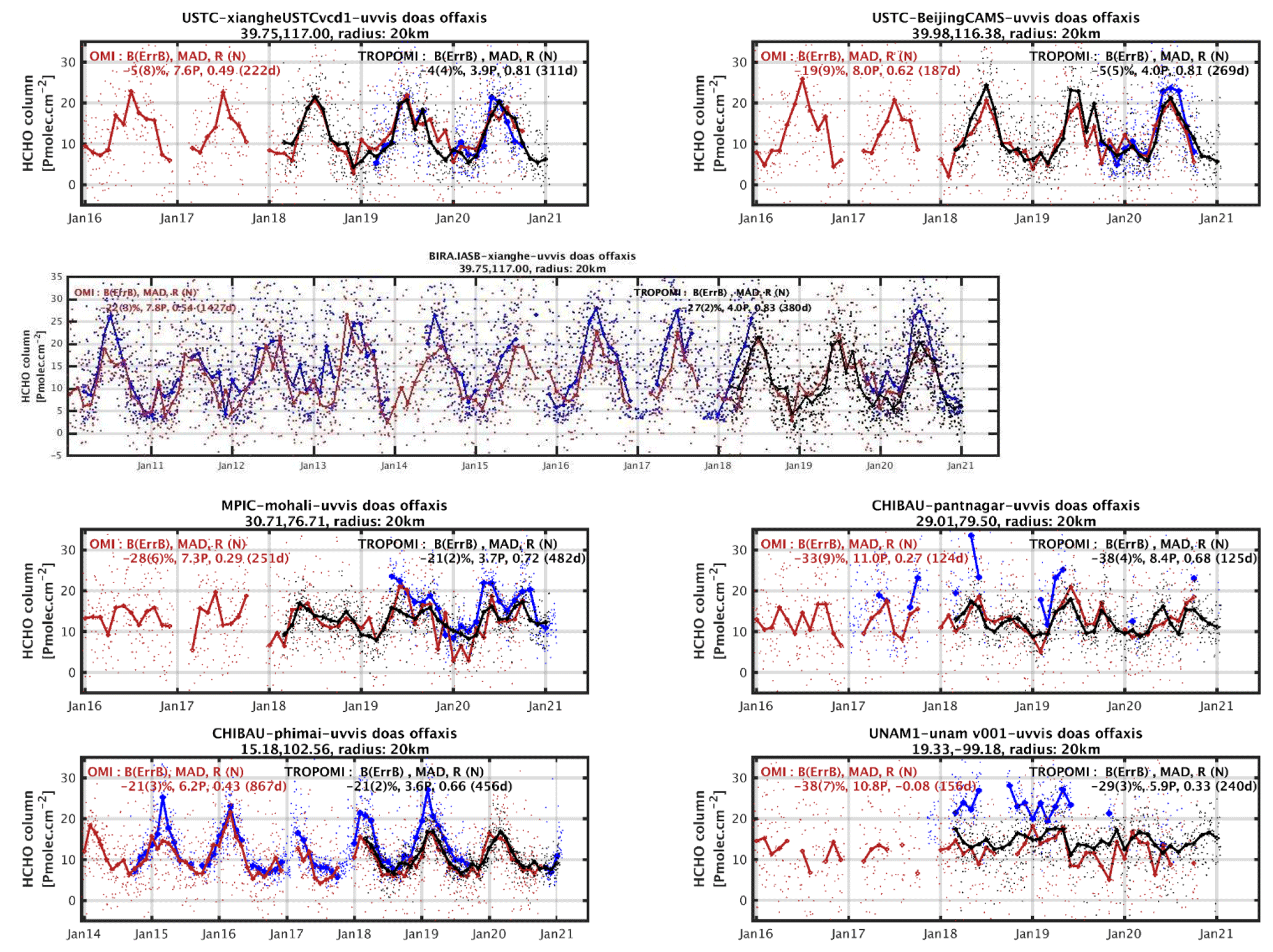
Stations with large HCHO levels in China, India, Thailand and Mexico are presented in Fig. 14. In China, we show the results of two instruments in Xianghe and one instrument in Beijing. With the USTC instruments, we find small biases of % and % and correlations larger than 0.8. With the BIRA-IASB instrument in Xianghe, the correlation is also excellent. The MAX-DOAS columns are larger than the ones obtained with the USTC instrument, and we find a significant negative bias of the TROPOMI data of %. However, this larger bias is in better agreement with the results found for equivalent stations in India and with FTIR validation results in Xianghe (Vigouroux et al., 2020). This result illustrates the actual uncertainty related to the ground-based measurements themselves and the need for further harmonization of the MAX-DOAS network. Correlations in India and Thailand are of about 0.7, while the biases are consistently negative ( % in Mohali, % in Pantnagar, % in Phimai). The situation is more complex at the UNAM site in Mexico. There, the correlation is poor (0.3), and a negative bias of % is found. These results are however more dependent on the radius considered around the station and on the selection of the MAX-DOAS observations (Rivera Cárdenas et al., 2021) (see Sect. 5.4).
Finally, Fig. 15 presents scatter plots of the satellite against MAX-DOAS columns, considering all the stations and for daily and monthly comparisons. Table 3 summarizes the validation results. The best agreement is found with monthly TROPOMI columns, for which we find a slope of 0.64 and a positive offset of 1.7 × 10¹⁵ molec. cm−2 compared to the MAX-DOAS columns. Slopes and biases for the large columns are found to be close for OMI and TROPOMI datasets. The improvement with TROPOMI can be seen in the correlation, offset and bias values obtained for the lower columns as well as in the precision of the daily validation results. On average, the OMI biases are found to be statistically non-significant for the lowest columns. When considering monthly averaged data, the correlation between MAX-DOAS and satellite columns improves from 0.74 with OMI to 0.85 with TROPOMI (+15 %). More importantly, it improves from 0.45 to 0.76 when considering daily observations (+68 %). The daily offset is reduced by 60 % from OMI to TROPOMI (3.1 to 1.9 × 10¹⁵ molec. cm−2). In low-emission conditions, the MADs of the differences provide an upper limit of the precision of the satellite measurements. If we consider HCHO levels below 8 × 10¹⁵ molec. cm−2 (medium level, but the low range is not represented here), the precision of the daily TROPOMI HCHO observations is estimated to be 3 × 10¹⁵ molec.cm−2, which represents an improvement of more than a factor 2 compared to OMI. The precision of monthly TROPOMI observations reaches 1.4 × 10¹⁵ molec. cm−2, which is close to the Copernicus user requirements.
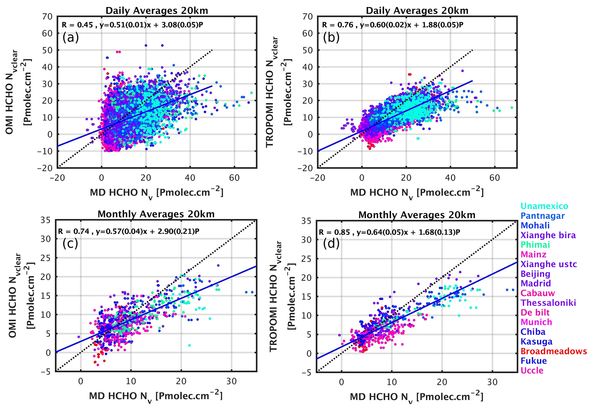
Figure 15Scatter plots of OMI (a, c) and TROPOMI (b, d) versus MAX-DOAS data for the daily (a, b) and monthly (c, d) medians of collocated data. The correlation, slope and intercept of a linear regression using the robust Theil–Sen estimator is given in each panel and plotted as a blue line. The black dotted line is the 1 : 1 line. The colour indicates the latitude of the station. (Pmolec. cm−2 = 1015 molec. cm−2.)
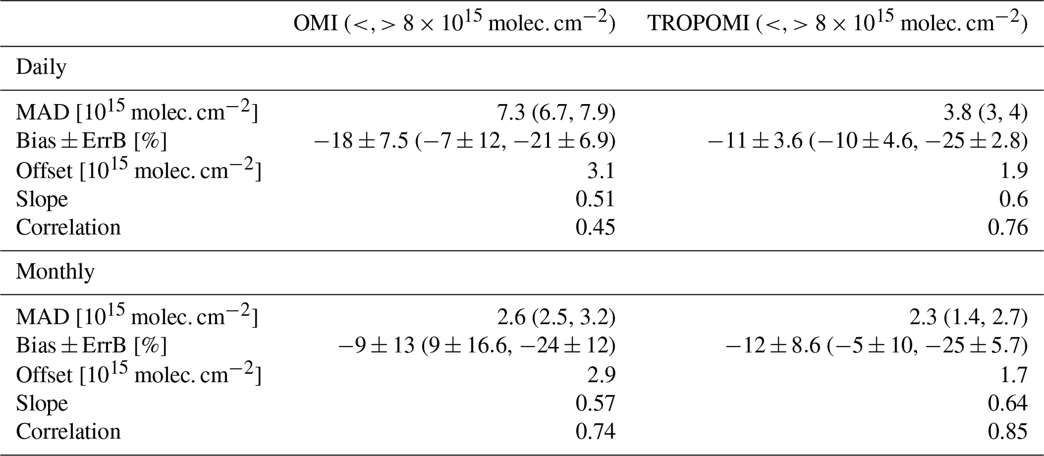
Table 3Summary of validation results for OMI and TROPOMI when considering all collocated pairs (daily or monthly means) together. Values for HCHO columns lower or larger than 8 × 10¹⁵ molec. cm−2 are given in brackets.
5.2 Sensitivity tests
We performed a few sensitivity tests, in order to evaluate the robustness of the validation results. First, we used different radii around the stations (from 10 to 100 km), in order to detect possible spatial resolution effects. Results are presented in Fig. 16, for the TROPOMI case. At most stations, the bias shows a marginally small dependency on the radius. Again, this points to the large natural dispersion of the HCHO columns. We find an important exception at the UNAM station in Mexico, where the bias clearly increases with the radius (−30 % at 10 km, −50 % at 100 km). At this location, the correlation and MADs are also improved at 10 km (not shown). In Beijing and Broadmeadows, we do observe an increase in the bias at 100 km resolution, but the values at 10 and 20 km are mostly equivalent. We performed the same test with OMI and found consistent results, except that the lower sampling does not allow using a 10 km radius area.

Figure 16Median monthly bias as a function of the radius taken around the validation sites. Pink areas indicate 40 % bias.
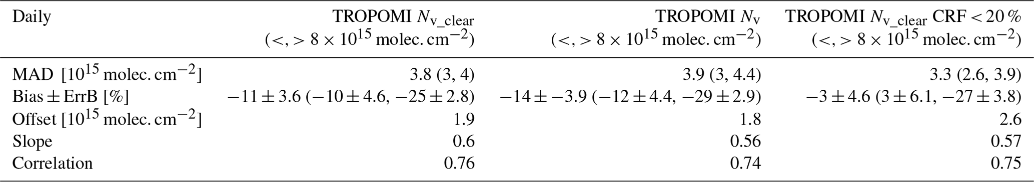
We also evaluated the impact of clouds using two further tests: (1) comparing the daily TROPOMI validation results for Nv and Nv_clear; (2) using a much stricter cloud filter on cloud radiance fractions (CRF) of 20 % instead of 60 % (equivalent to an effective cloud fraction of 10 % instead of 40 %). With this strict cloud filter, there is no difference between Nv and Nv_clear. Results are summarized in Table 4. These tests indicate that the TROPOMI HCHO validation results do not change significantly when a cloud correction is applied, although the Nv_clear results are slightly better. Using a more stringent cloud filter reduces the number of observations. The bias for the lowest columns becomes positive (from −10 to +3 %), and the offset is increased (from 1.9 to 2.6 × 10¹⁵ molec. cm−2), while the negative bias for the largest columns remains equivalent. These numbers will have to be re-evaluated using only version 2 of the TROPOMI level 2 products, available since July 2020, when enough data will be available. However, we note that this limited impact of the cloud correction on the HCHO columns appears to be consistent with previous satellite datasets, independently of the cloud product, as already observed with GOME-2 and OMI, using version 1 of the O2–O2 cloud product (De Smedt et al., 2015).
Table 4Summary of daily validation results for TROPOMI when considering all collocated pairs when using (baseline) Nv_clear (first column), (1) when using Nv (second column) or (2) when using a strict cloud filter (third column).
5.3 Effect of vertical smoothing
Three MAX-DOAS stations (Uccle, Xianghe BIRA-IASB and UNAM) provide retrieved and a priori vertical profiles together with corresponding averaging kernels (GEOMS format, https://evdc.esa.int/tools/data-formatting-templates/, last access: 18 August 2021). This allows taking into account the different vertical sensitivity of MAX-DOAS and TROPOMI measurements when making comparisons. We follow the methodology from Rodgers and Connor (2003) described in detail in Vigouroux et al. (2020). It consists of two steps: first taking into account the different a priori profiles used to retrieve these two data sets (Eq. 2 of Vigouroux et al., 2020) and then smoothing the ground-based profiles using TROPOMI averaging kernels (Eq. 3 of Vigouroux et al., 2020).
In Table 5, we give the MAD and biases obtained before and after application of the methodology, for the daily mean comparisons. Note that the numbers at each site are slightly different than the ones obtained in Sect. 5.1 (Figs. 12 and 14) because the collocated pairs are constructed slightly differently: each collocated pixel of the satellite must be compared to MAX-DOAS before the daily average because the TROPOMI averaging kernel differs for each pixel.
We see in Table 5 that at the cleanest site (Uccle) the effect of the smoothing is small, while at the more polluted sites Xianghe and UNAM, the biases are strongly reduced by about 20 %. This result is in agreement with previous MAX-DOAS validation studies (De Smedt et al., 2015; Wang et al., 2019b), but also with aircraft and regional model comparisons (Zhu et al., 2020; Su et al., 2020). The effect of the smoothing is also clearly seen in Fig. 17 where the scatter plots of daily comparisons between TROPOMI and MAX-DOAS are shown before and after vertical smoothing. The strong effect of the smoothing is usually not observed with FTIR comparisons because TROPOMI and FTIR measurements have similar vertical sensitivity, which rapidly drops in the atmospheric layers lower than 3 km (Vigouroux et al., 2020), while MAX-DOAS shows an opposite sensitivity that is maximal at the surface and generally becomes negligible above 3 km (Vigouroux et al., 2009; De Smedt et al., 2015; Wang et al., 2019a). An illustration of typical averaging kernels for OMI, TROPOMI and the MAX-DOAS instrument in Xianghe is provided in Fig. S6. As the observation angles and overpass times are very close for OMI and TROPOMI, their measurements come with a similar vertical sensitivity. This highlights the importance of taking into account the different a priori profiles and averaging kernels when comparing techniques having different vertical sensitivity.
Table 5Effect of a priori substitution and vertical smoothing on the daily comparisons of TROPOMI and MAX-DOAS data.

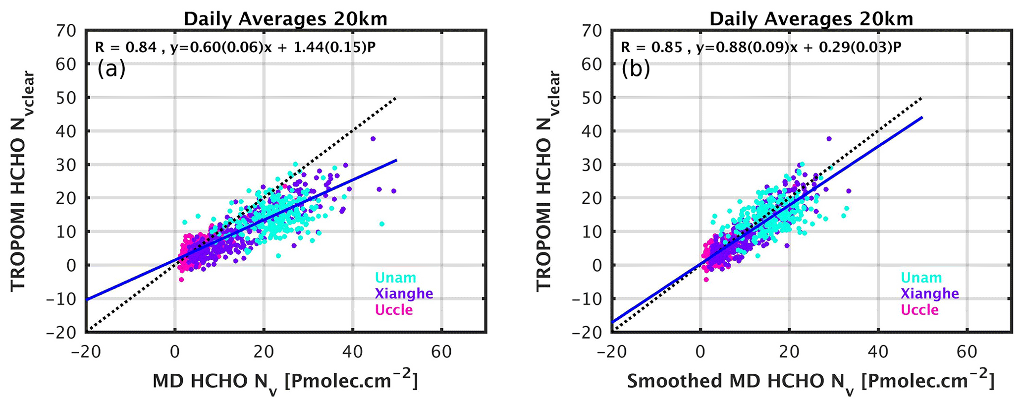
Figure 17Scatter plots of TROPOMI versus MAX-DOAS data for the daily means of collocated data before (a) and after (b) vertical smoothing of the MAX-DOAS profile in Uccle, Xianghe and UNAM, Mexico. The correlation, slope and intercept of a linear regression using the robust Theil–Sen estimator is given in each panel and plotted as a blue line. The black dotted line is the 1 : 1 line (Pmolec. cm−2 = 1015 molec. cm−2).
As shown above, TROPOMI HCHO observations feature an unprecedented level of precision allowing for an improved detection of small columns at short timescales. Here, we present a case study to illustrate the ability of TROPOMI to detect small HCHO signals related to shipping emissions. When inspecting TROPOMI maps averaged over several months, weak lines of HCHO columns become visible over the background, especially in the Indian Ocean (see e.g. Fig. 5). This becomes even clearer when saturating the continental HCHO columns by setting a lower maximum scale, as in Fig. 18, which shows HCHO columns seasonally averaged over the months December, January and February between 2018 and 2021.
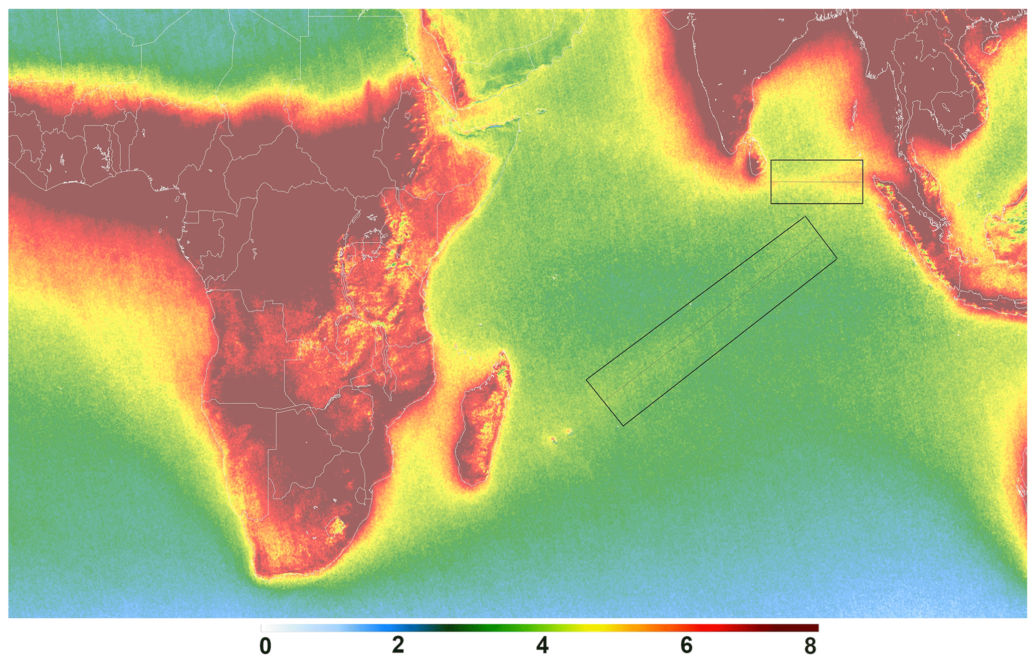
Figure 18Seasonal DJF map of TROPOMI HCHO tropospheric columns between December 2018 and February 2021, on a spatial grid of 0.05∘ in latitude and longitude. Observations are only filtered using the provided qa_values > 0.5 (max scale: 8 × 10¹⁵ molec. cm−2).
The detection of shipping emissions with satellite observations has often been reported for NO2 (see for example Beirle et al., 2004; Richter et al., 2004, 2011; Boersma et al., 2015; Georgoulias et al., 2020) and more recently also for SO2 based on OMI measurements (Theys et al., 2015). In the case of HCHO, however, only one study pointed to the identification of a shipping lane signal detected in a 7-year average of ERS-2 GOME data in the ship track corridor from Sri Lanka to Singapore (Marbach et al., 2009).
Here, we study two lines: (1) from Sri Lanka to Singapore and (2) from Madagascar to Singapore. We perform an analysis and several sensitivity tests in order to gain confidence and information on the enhanced HCHO. As illustrated in Fig. 19a (line 1) and Fig. 20a (line 2), in each box, we average the HCHO columns along the ship track to obtain a spatial cross section, and we bin the data as a function of the distance from the line (distances are expressed in degrees per 0.5∘ bin). The background level is not constant, for example due to continental outflow in the Bay of Bengal, and needs to be removed. To do so, we fit a straight line through the column values at the edges of the box and subtract this line from the signal. This allows us to isolate a differential column and to evaluate its absolute and relative magnitude compared to the background (respectively, shown in Figs. 19b, c and 20b, c). For comparison, we perform the same analysis using TROPOMI NO2 tropospheric columns from the operational product (NO2 ATBD, https://sentinel.esa.int/documents/247904/2476257/Sentinel-5P-TROPOMI-ATBD-NO2-data-products, last access: 18 August 2021, Van Geffen et al., 2020). Although only about half as wide, the localization of the NO2 peak is found to be well aligned with the HCHO signal. Along the line from Sri Lanka to Singapore, we find a similar column enhancement and plume width as in Marbach et al. (2009).
In order to exclude a possible indirect AMF effect caused by the TM5 a priori profiles, the same analysis is done based on background-corrected slant columns (bc-SCDs). We also restrict the analysis to clear-sky observations by using a strict cloud filtering of CRF < 20 %. Furthermore, we use the wind vector information provided in the TROPOMI L2 product from version 2 onwards (from August 2020) to select only clear-sky observations with low-wind conditions (qa > 0.5, CRF < 20 %, W<5 m s−1). Finally, we add to the analysis a climatology of HCHO observations based on OMI measurements (2005–2009).
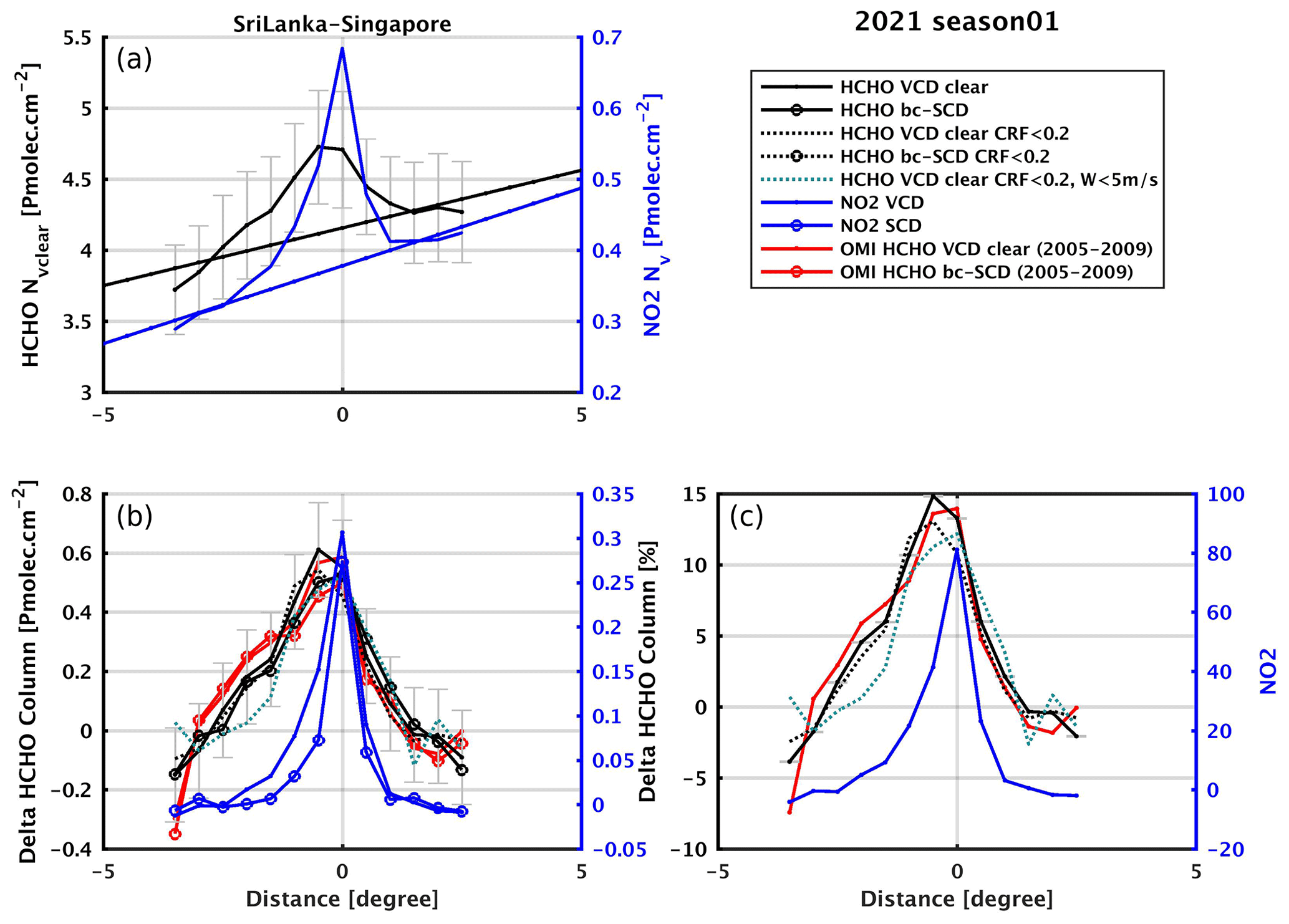
Figure 19Box average for the first selected line between Sri Lanka and Singapore between December 2020 and February 2021. The x axis represents the distance (south–north) in degrees from the shipping lane. Panel (a) shows the HCHO (in black) and NO2 (in blue) tropospheric columns, binned per distance from the line centre. The fitted lines are used to remove the background contribution. The two bottom panels present the absolute (b) and relative (c) column deviations from the background line. The analysis is performed on the slant and the vertical columns (circles/lines), using a stricter cloud filtering (CRF < 20 %, black dotted line) and an additional filter on the wind velocity (W<5 m s−1, green dotted line) and finally on OMI observations averaged between 2005 and 2009 (red). (Pmolec. cm−2 = 1 × 10¹⁵ molec. cm−2.)
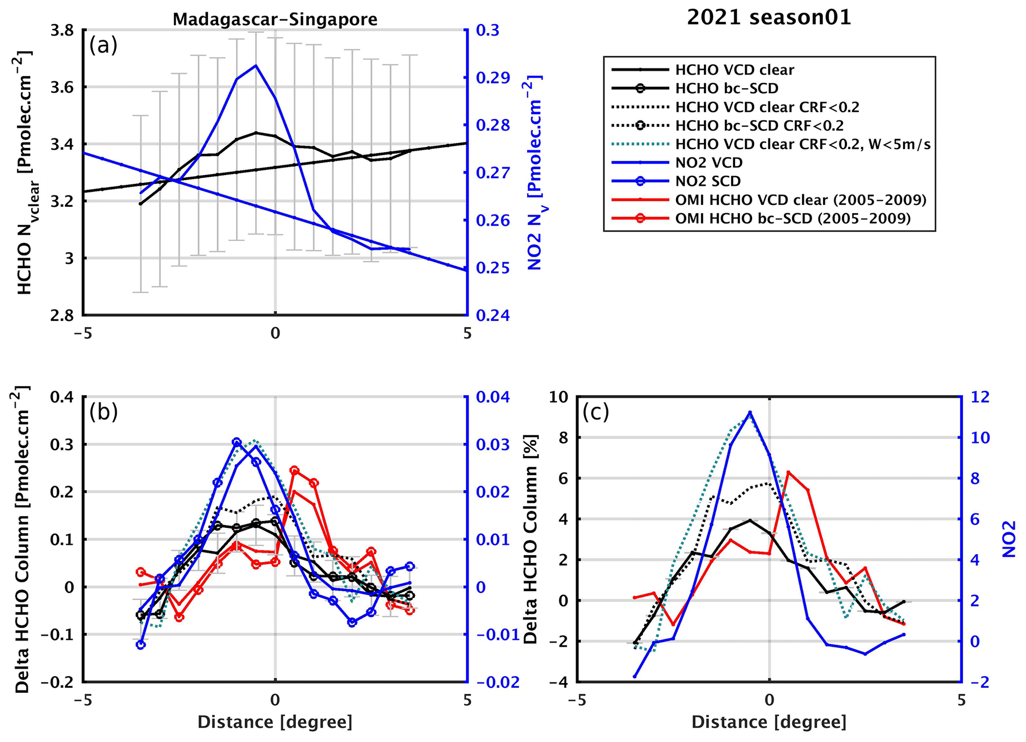
Using this approach, we analysed HCHO datasets for each season between MAM 2018 and DJF 2021. The absolute and relative magnitude of the largest detected signal is plotted as a function of the season in Figs. 21 and 22. Along the two lines, the signal is detected in the slant columns of HCHO and NO2 as well. This excludes the possibility of an artefact coming from the TM5 a priori profiles. The signal remains detectable in clear-sky observations and is even increased along the second line. We observe a similar effect of the wind speed filtering (last two seasons). Selecting only low-wind conditions clearly enhances the signal along line 2 and during SON along line 1. The magnitude of the detected HCHO signal is larger along line 1 (from 0.2 to 0.7 × 10¹⁵ molec. cm−2, 15 %) compared to line 2 (from 0.1 to 0.3 × 10¹⁵ molec. cm−2, 8 %). We find that the absolute magnitude of the HCHO signal is larger than the NO2 signal by a factor of 3 to 10, but the relative increase in the NO2 columns is significantly larger: 60 % along line 1 and 15 % along line 2. Both lines show a clear seasonality, particularly in the HCHO columns, with a maximum during the DJF seasons seen in the OMI climatology and in the TROPOMI 3-month averages. The HCHO signal presents a clear drop in JJA along line 1. This is related to the wind direction and strength, which bring the line signal closer to the HCHO continental outflow, making its detection more difficult. The OMI data need to be averaged over several years in order to detect a significant signal. While the first line is well detected in the 5-year OMI climatology, the second line presents a smaller magnitude and a larger variability and cannot be detected in the most recent years of OMI measurements.
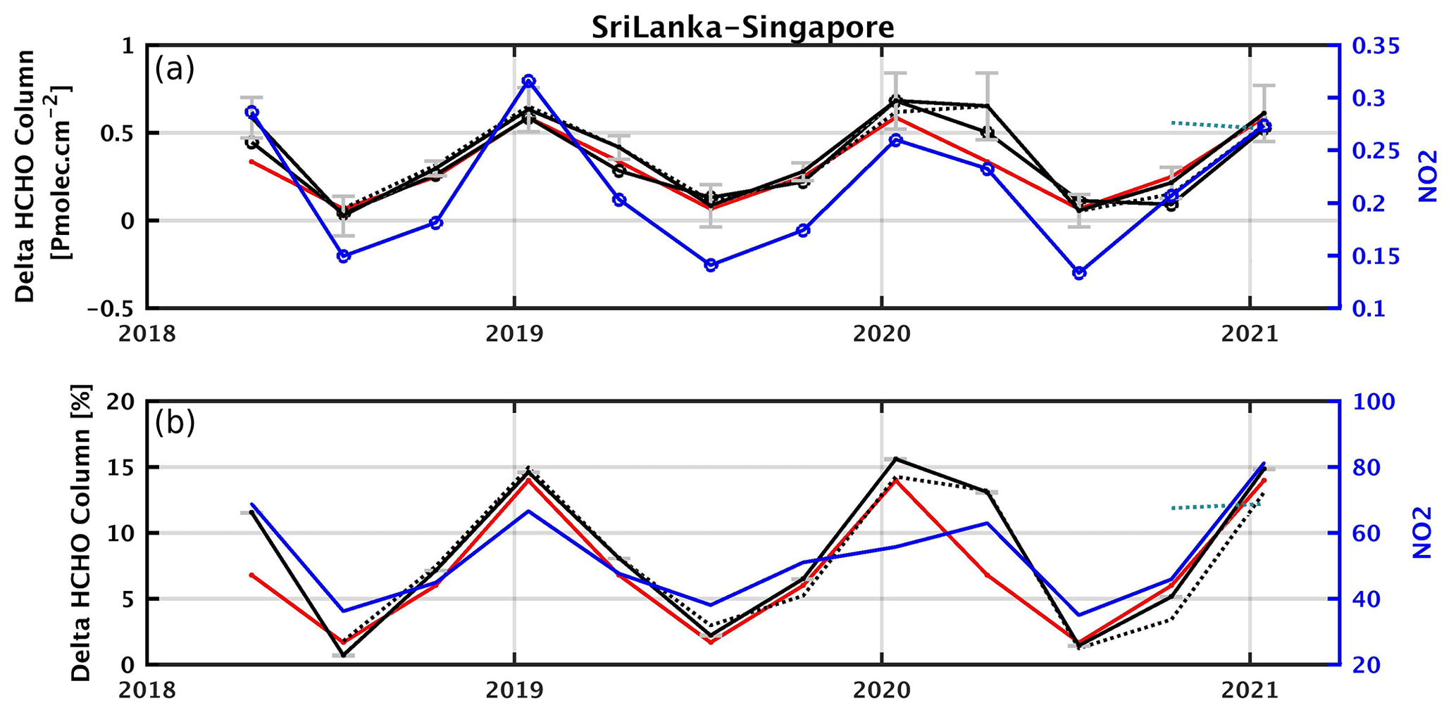
Figure 21Seasonal variation in the absolute (a) and relative (b) column deviations of the TROPOMI HCHO (black), OMI 2005–2009 climatology HCHO (red) and TROPOMI NO2 (blue) tropospheric columns along the Sri Lanka–Singapore line. For each season, the maximum deviation compared to the background is provided. The results of the analysis are given for the slant and the vertical columns (circles/lines), using a stricter cloud filtering (CRF < 20 %, black dotted line) and an additional filter on the wind velocity (W<5 m s−1, green dotted line). (Pmolec. cm−2 = 1 × 10¹⁵ molec. cm−2.)
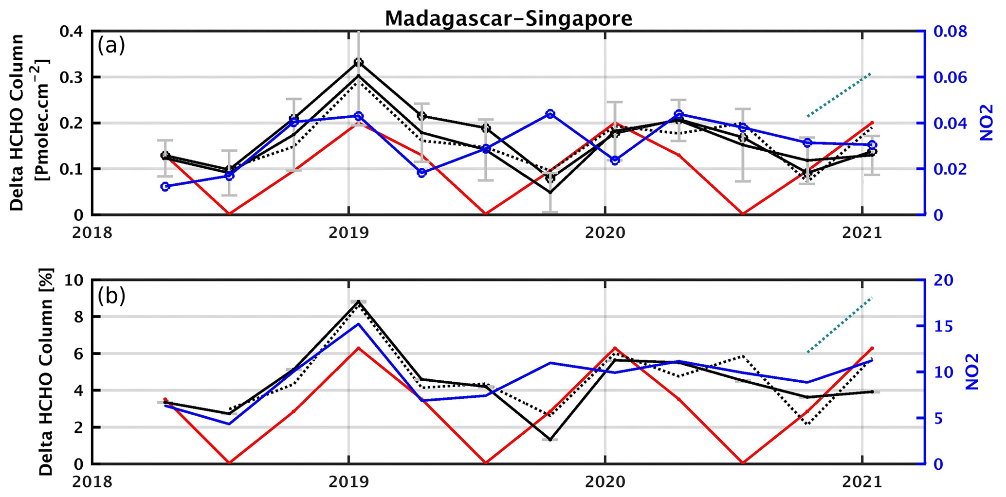
Using TROPOMI HCHO observations averaged over 3 months, it is therefore possible to detect a signal as small as 0.1 × 10¹⁵ molec. cm−2 (with a median deviation of 0.03 × 10¹⁵ molec. cm−2), after removal of the background contribution. Note that along the first line a similar analysis can also be performed on a monthly basis. While we show several pieces of evidence that the signal is related to shipping emissions, its source is not studied here. As discussed in Marbach et al. (2009) it could be due to secondary HCHO production via the atmospheric oxidation of NMVOCs emitted from ship engines but also to enhanced CH4 oxidation by elevated levels of OH radicals within the ship plumes. Model analysis suggests that the second hypothesis is the main factor responsible for the elevated HCHO levels (Song et al., 2010). Other HCHO lines can be detected as well in the tropics, although weaker in magnitude or closer to the continental outflow (in the south-west of Africa or in the west of India). More advanced techniques to separate the signal from the background and to account for wind dispersion effects could help in detecting more shipping lanes but also weak continental emissions (Beirle et al., 2004).
Owing to its high spatial resolution resulting in many measurement points, coupled with an improved signal-to-noise ratio at the single-pixel level, TROPOMI allows us to monitor HCHO tropospheric columns from space with an unprecedented definition. The global and regional maps show a clear reduction in the noise compared to previous sensors, allowing for the detection of weaker HCHO signals and the monitoring of HCHO variations on a much shorter timescale.
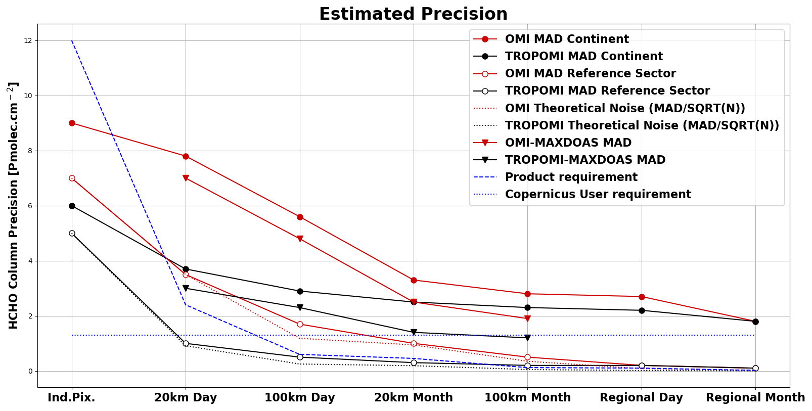
Figure 23Estimated precision of OMI (in red) and TROPOMI (in black) HCHO columns at different spatial and temporal scales (20 km, 100 km, regions, day, month). The median deviation of the satellite HCHO columns are provided for continental emissions (plain circles) and in the remote reference sector (white circles). Validation estimates are plotted at 20 and 100 km (MAD of differences between satellite and MAX-DOAS columns, triangles). The theoretical noise (dotted lines) corresponds to single-measurement precision divided by the square root of observations. The dashed blue line is the TROPOMI product requirement, based on a single-measurement precision of 12 × 1015 molec. cm−2. The horizontal blue line at 1.3 × 10¹⁵ molec. cm−2 represents the Copernicus user requirement. (Pmolec. cm−2 = 1 × 10¹⁵ molec. cm−2.)
We have evaluated the TROPOMI HCHO operational product against the QA4ECV OMI HCHO dataset and against a network of 18 ground-based MAX-DOAS instruments. The gain in precision at different spatial and temporal scales was estimated by (1) comparing the median deviation of the averaged columns and (2) validating the data using MAX-DOAS column network measurements. Both methods include additional noise components from temporal variation, spatial variation and ground-based column precision. Results are summarized in Fig. 23 where precision estimates are provided for observations over regions with enhanced continental emissions and for background conditions, as a function of the time resolution (daily or monthly averages) and of the spatial resolution (from 20 km to regional scale). At 20 and 100 km resolution, both the median deviation approach and the validation results lead to very consistent estimates of the precision. The theoretical noise is also represented in the figure; it decreases as the squared root of the number of observations included in the averages. In remote conditions, the median deviation of the averaged columns follows closely the theoretical noise until reaching a threshold. If we consider a large region in the reference sector, all estimates converge towards a limit of about 0.2 × 10¹⁵ molec. cm−2 (day) to 0.1 × 10¹⁵ molec. cm−2 (month) both for OMI and TROPOMI. Over continental emission sources, the reduction in the noise is counterbalanced by the HCHO natural variability and by other sources of pseudo-noise which depend on the spatial and temporal scales of the observations. The largest improvement brought by TROPOMI is found for daily observations at 20 km resolution, for which a gain in precision by a factor of 3 is obtained compared to OMI. The product and Copernicus user requirements for precision are also represented in the figure. Both are reached with TROPOMI using daily averaged data at the resolution of 20 km if we consider the dispersion in remote regions. However, over continental emissions, local variability effects added up to the estimated precision that reaches a threshold of about 2 × 10¹⁵ molec. cm−2.
For the HCHO absolute values, we show that OMI and TROPOMI observations agree very well for moderate to large HCHO levels (columns larger than 5 × 10¹⁵ molec. cm−2) for which the bias between both datasets is smaller than 10 %. For lower columns, however, OMI observations present a remaining bias of about +20 % compared to TROPOMI. This good agreement is obtained by considering vertical columns calculated with air mass factors not corrected for cloud effects (clear VCD). This allows us to avoid biases related to differences in the cloud products. For all applications that require combining the OMI and TROPOMI observations for low to moderate cloud fractions, we therefore advise using clear VCDs. Validation results confirm the good agreement between the OMI and TROPOMI datasets and a similar underestimation of both products in the highest range of the HCHO levels (−25 % on average for columns larger than 8 × 10¹⁵ molec. cm−2). For medium columns, OMI presents a slight overestimation compared to MAX-DOAS data, which is not observed for TROPOMI. Sensitivity tests show that validation results obtained with the TROPOMI HCHO columns are weakly dependent on the cloud correction. They also depend weakly on the radius considered around the station, with a few exceptions such as Mexico city or coastal stations. By contrast, the vertical smoothing (tested at three stations) has a strong effect on the comparison with MAX-DOAS. After taking into account the different a priori profiles and averaging kernels, the bias for large HCHO columns is strongly reduced by about 20 %.
Comparing OMI and TROPOMI monthly averaged HCHO columns, we do not observe significant differences related to the spatial resolution, except in regions surrounded by natural boundaries where the benefit of the finer spatial resolution of TROPOMI is clearly apparent. The weak sensitivity to the spatial resolution of HCHO measurements can be understood when considering that HCHO is a secondary product from the degradation of NMVOCs with various lifetimes, which results in a general spread of the HCHO spatial distributions. The large number of TROPOMI observations allows us to perform validation at a resolution as small as 10 km on a daily basis with a sufficient precision, which is not possible with OMI. It is clear that TROPOMI brings a significant improvement in the temporal resolution of the observations. At most of the validation sites, TROPOMI allows for daily validation results as robust as those obtained with OMI on a monthly basis.
The number of ground-based stations providing MAX-DOAS HCHO observations is constantly growing, providing a large range of observation conditions and for some of them allowing comparisons of the performances of several satellite datasets over several years. Note however that the lower range of HCHO levels is underrepresented as are some of the largest emission regions such as South America or Africa. Following the validation study of Vigouroux et al. (2020) based on an FTIR network of instruments, this study illustrates again the added value of using a large network of instruments to draw more robust conclusions. FTIR and MAX-DOAS networks are complementary to each other and could be combined to cover as many conditions as possible. Similarly to what was achieved for the FTIR network, the MAX-DOAS HCHO datasets would benefit from further homogenization efforts.
Finally, to illustrate the benefit of TROPOMI for the detection of small HCHO signals, we present a case study addressing the detection of shipping lanes in the Indian Ocean. Using simultaneous observations of tropospheric NO2 and meteorological wind field data, we present strong evidence for an HCHO production in regions affected by shipping emissions. Owing to the fine spatial resolution and high spatial sampling of TROPOMI, such small signals can now be observed from space on a seasonal basis.
The S5p HCHO data are available at https://doi.org/10.5270/S5P-tjlxfd2 (Copernicus Sentinel-5P, 2018). The dataset is a Copernicus operational product. Users have to log in to https://s5phub.copernicus.eu/dhus/#/home (last access: 18 August 2021). The access and use of any Copernicus Sentinel data available through the Copernicus Sentinel Data Hub is governed by the Legal Notice on the use of Copernicus Sentinel Data and Service Information and is given here: https://sentinels.copernicus.eu/documents/247904/690755/Sentinel_Data_Legal_Notice (last access: 18 August 2021).
The QA4ECV OMI HCHO product is available at https://doi.org/10.18758/71021031 (De Smedt et al., 2017). The MAX-DOAS datasets can be requested from the individual PIs of each station.
The supplement related to this article is available online at: https://doi.org/10.5194/acp-21-12561-2021-supplement.
IDS coordinated the paper and carried out the analysis. GP and CV are PIs of the NIDFORVAL S5PVT project; SC ensures the MPC routine validation. IDS, PH, YH, CLe, DL, FR, NT, JV and MVR developed the TROPOMI HCHO product. FB, IDS, YH, AR, MVR and TWag developed the QA4ECV OMI HCHO product. AB, NB, KLC, SD, FH, HI, VK, CLi, AP, CRC, RGR, MVR and TWan are PIs for the QA4ECV MAX-DOAS measurements. BL, SC, GP and CV performed MAX-DOAS data collection and format harmonization and carried out the validation analysis. SC, KUE and JCL are responsible for the MPC routine validation. MVR is the coordinator of this research. All co-authors revised and commented on the paper.
Andreas Richter, Thomas Wagner and Michel Van Roozendael are editors of the journal.
Publisher’s note: Copernicus Publications remains neutral with regard to jurisdictional claims in published maps and institutional affiliations.
This work contains modified Copernicus Sentinel-5 Precursor satellite data (2018–2020) post-processed by BIRA-IASB. We acknowledge Mark Wenig from LMU for supporting the MAX-DOAS operations in Munich, Caroline Fayt and Christian Herman from BIRA-IASB for the Uccle and Xianghe instruments, and Pucaï Wang from IAP/CAS for maintaining the BIRA-IASB instrument in Xianghe. We thank Alejandro Bezanilla from CCA-UNAM, Manish Naia from ARIES for the MAX-DOAS instrument operation in Pantnager, and Thanawat Jarupongsakul from Chulalongkorn University for the Phimai station. We acknowledge IISER Mohali Atmospheric Chemistry Facility for supporting the MAX-DOAS operations in Mohali.
Part of the reported work was carried out in the framework of the Copernicus Sentinel-5 Precursor Mission Performance Centre (S5p MPC), contracted by the European Space Agency (ESA/ESRIN, contract no. 4000117151/16/I-LG) and supported by the Belgian Federal Science Policy Office (BELSPO), the Royal Belgian Institute for Space Aeronomy (BIRA-IASB) and the German Aerospace Centre (DLR). BIRA-IASB acknowledges national funding from BELSPO and ESA through the ProDEx projects TRACE-S5P (TRACE-S5P project) and TROVA. Part of this work was also carried out in the framework of the S5p Validation Team (S5PVT) AO projects NIDFORVAL (ID no. 28607, PI Gaia Pinardi, Corinne Vigouroux, BIRA-IASB). Multi-sensor HCHO developments have been funded by the EU FP7 QA4ECV project (grant no. 607405), in close cooperation with KNMI, University of Bremen, MPIC-Mainz and WUR. Work by Hitoshi Irie was supported by the Environment Research and Technology Development Fund (JPMEERF20192001 and JPMEERF20215005) of the Environmental Restoration and Conservation Agency of Japan, JSPS KAKENHI (grant numbers JP19H04235 and JP20H04320) and the JAXA 2nd Research Announcement on the Earth Observations (grant number 19RT000351).
This paper was edited by Andreas Hofzumahaus and reviewed by two anonymous referees.
Alvarado, L. M. A., Richter, A., Vrekoussis, M., Hilboll, A., Kalisz Hedegaard, A. B., Schneising, O., and Burrows, J. P.: Unexpected long-range transport of glyoxal and formaldehyde observed from the Copernicus Sentinel-5 Precursor satellite during the 2018 Canadian wildfires, Atmos. Chem. Phys., 20, 2057–2072, https://doi.org/10.5194/acp-20-2057-2020, 2020.
Arellano, J., Krüger, A., Rivera, C., Stremme, W., Friedrich, M., Bezanilla, A., and Grutter, M.: The MAX-DOAS network in Mexico City to measure atmospheric pollutants, Atmosfera, 29, 157–167, https://doi.org/10.20937/ATM.2016.29.02.05, 2016.
Barkley, M. P., González Abad, G., Kurosu, T. P., Spurr, R., Torbatian, S., and Lerot, C.: OMI air-quality monitoring over the Middle East, Atmos. Chem. Phys., 17, 4687–4709, https://doi.org/10.5194/acp-17-4687-2017, 2017.
Bauwens, M., Stavrakou, T., Müller, J.-F., De Smedt, I., Van Roozendael, M., van der Werf, G. R., Wiedinmyer, C., Kaiser, J. W., Sindelarova, K., and Guenther, A.: Nine years of global hydrocarbon emissions based on source inversion of OMI formaldehyde observations, Atmos. Chem. Phys., 16, 10133–10158, https://doi.org/10.5194/acp-16-10133-2016, 2016.
Beirle, S., Platt, U., von Glasow, R., Wenig, M., and Wagner, T.: Estimate of nitrogen oxide emissions from shipping by satellite remote sensing, Geophys. Res. Lett., 31, L18102, https://doi.org/10.1029/2004GL020312, 2004.
Beirle, S., Borger, C., Dörner, S., Li, A., Hu, Z., Liu, F., Wang, Y., and Wagner, T.: Pinpointing nitrogen oxide emissions from space, Sci. Adv., 5, eaax9800, https://doi.org/10.1126/sciadv.aax9800, 2019.
Benavent, N., Garcia-Nieto, D., Wang, S., and Saiz-Lopez, A.: MAX-DOAS measurements and vertical profiles of glyoxal and formaldehyde in Madrid, Spain, Atmos. Environ., 199, 357–367, https://doi.org/10.1016/j.atmosenv.2018.11.047, 2019.
Boersma, K. F., Eskes, H. J., and Brinksma, E. J.: Error analysis for tropospheric NO2 retrieval from space, J. Geophys. Res., 109, D04311, https://doi.org/10.1029/2003JD003962, 2004.
Boersma, K. F., Vinken, G. C. M., and Tournadre, J.: Ships going slow in reducing their NOx emissions: changes in 2005–2012 ship exhaust inferred from satellite measurements over Europe, Environ. Res. Lett., 10, 074007, https://doi.org/10.1088/1748-9326/10/7/074007, 2015.
Boersma, K. F., Eskes, H. J., Richter, A., De Smedt, I., Lorente, A., Beirle, S., van Geffen, J. H. G. M., Zara, M., Peters, E., Van Roozendael, M., Wagner, T., Maasakkers, J. D., van der A, R. J., Nightingale, J., De Rudder, A., Irie, H., Pinardi, G., Lambert, J.-C., and Compernolle, S. C.: Improving algorithms and uncertainty estimates for satellite NO2 retrievals: results from the quality assurance for the essential climate variables (QA4ECV) project, Atmos. Meas. Tech., 11, 6651–6678, https://doi.org/10.5194/amt-11-6651-2018, 2018.
Bösch, T., Rozanov, V., Richter, A., Peters, E., Rozanov, A., Wittrock, F., Merlaud, A., Lampel, J., Schmitt, S., de Haij, M., Berkhout, S., Henzing, B., Apituley, A., den Hoed, M., Vonk, J., Tiefengraber, M., Müller, M., and Burrows, J. P.: BOREAS – a new MAX-DOAS profile retrieval algorithm for aerosols and trace gases, Atmos. Meas. Tech., 11, 6833–6859, https://doi.org/10.5194/amt-11-6833-2018, 2018.
Bovensmann, H., Peuch, V.-H., van Weele, M., Erbertseder, T., and Veihelmann, B.: Report Of The Review Of User Requirements For Sentinels-4/-5, ESA, EOP-SM/2281/BV-bv, issue: 1.2, ESA, 2011.
Brinksma, E. J., Pinardi, G., Volten, H., Braak, R., Richter, A., Scho, A., Van Roozendael, M., Fayt, C., Hermans, C., Dirksen, R. J., Vlemmix, T., Berkhout, A. J. C., Swart, D. P. J., Oetjen, H., Wittrock, F., Wagner, T., Ibrahim, O. W., Leeuw, G. De, Moerman, M., Curier, R. L., Celarier, E. A., Cede, A., Knap, W. H., Veefkind, J. P., Eskes, H. J., Allaart, M., Rothe, R., Piters, A., and Levelt, P. F.: The 2005 and 2006 DANDELIONS NO2 and aerosol intercomparison campaigns, J. Geophys. Res., 113, 1–18, https://doi.org/10.1029/2007JD008808, 2008.
Cao, H., Fu, T.-M., Zhang, L., Henze, D. K., Miller, C. C., Lerot, C., Abad, G. G., De Smedt, I., Zhang, Q., van Roozendael, M., Hendrick, F., Chance, K., Li, J., Zheng, J., and Zhao, Y.: Adjoint inversion of Chinese non-methane volatile organic compound emissions using space-based observations of formaldehyde and glyoxal, Atmos. Chem. Phys., 18, 15017–15046, https://doi.org/10.5194/acp-18-15017-2018, 2018.
Chan, K. L., Wang, Z., Ding, A., Heue, K.-P., Shen, Y., Wang, J., Zhang, F., Shi, Y., Hao, N., and Wenig, M.: MAX-DOAS measurements of tropospheric NO2 and HCHO in Nanjing and a comparison to ozone monitoring instrument observations, Atmos. Chem. Phys., 19, 10051–10071, https://doi.org/10.5194/acp-19-10051-2019, 2019.
Chan, K. L., Wiegner, M., van Geffen, J., De Smedt, I., Alberti, C., Cheng, Z., Ye, S., and Wenig, M.: MAX-DOAS measurements of tropospheric NO2 and HCHO in Munich and the comparison to OMI and TROPOMI satellite observations, Atmos. Meas. Tech., 13, 4499–4520, https://doi.org/10.5194/amt-13-4499-2020, 2020.
Chance, K. V., Palmer, P. I., Martin, R. V., Spurr, R. J. D., Kurosu, T. P., and Jacob, D. J.: Satellite observations of formaldehyde over North America from GOME, Geophys. Res. Lett., 27, 3461–3464, https://doi.org/10.1029/2000GL011857, 2000.
Chan Miller, C., Jacob, D. J., Marais, E. A., Yu, K., Travis, K. R., Kim, P. S., Fisher, J. A., Zhu, L., Wolfe, G. M., Hanisco, T. F., Keutsch, F. N., Kaiser, J., Min, K.-E., Brown, S. S., Washenfelder, R. A., González Abad, G., and Chance, K.: Glyoxal yield from isoprene oxidation and relation to formaldehyde: chemical mechanism, constraints from SENEX aircraft observations, and interpretation of OMI satellite data, Atmos. Chem. Phys., 17, 8725–8738, https://doi.org/10.5194/acp-17-8725-2017, 2017.
Choi, Y. and Souri, A. H.: Seasonal behavior and long-term trends of tropospheric ozone, its precursors and chemical conditions over Iran: A view from space, Atmos. Environ., 106, 232–240, https://doi.org/10.1016/j.atmosenv.2015.02.012, 2015.
Clémer, K., Van Roozendael, M., Fayt, C., Hendrick, F., Hermans, C., Pinardi, G., Spurr, R., Wang, P., and De Mazière, M.: Multiple wavelength retrieval of tropospheric aerosol optical properties from MAXDOAS measurements in Beijing, Atmos. Meas. Tech., 3, 863–878, https://doi.org/10.5194/amt-3-863-2010, 2010.
Compernolle, S., Argyrouli, A., Lutz, R., Sneep, M., Lambert, J.-C., Fjæraa, A. M., Hubert, D., Keppens, A., Loyola, D., O'Connor, E., Romahn, F., Stammes, P., Verhoelst, T., and Wang, P.: Validation of the Sentinel-5 Precursor TROPOMI cloud data with Cloudnet, Aura OMI O2–O2, MODIS, and Suomi-NPP VIIRS, Atmos. Meas. Tech., 14, 2451–2476, https://doi.org/10.5194/amt-14-2451-2021, 2021.
Copernicus Sentinel-5P (processed by ESA): TROPOMI Level 2 Formaldehyde Total Column products, Version 01, European Space Agency [data set], https://doi.org/10.5270/S5P-tjlxfd2, 2018.
De Smedt, I., Müller, J.-F., Stavrakou, T., van der A, R., Eskes, H., and Van Roozendael, M.: Twelve years of global observations of formaldehyde in the troposphere using GOME and SCIAMACHY sensors, Atmos. Chem. Phys., 8, 4947–4963, https://doi.org/10.5194/acp-8-4947-2008, 2008.
De Smedt, I., Stavrakou, T., Müller, J. F., van Der A, R. J., and Van Roozendael, M.: Trend detection in satellite observations of formaldehyde tropospheric columns, Geophys. Res. Lett., 37, L18808, https://doi.org/10.1029/2010GL044245, 2010.
De Smedt, I., Van Roozendael, M., Stavrakou, T., Müller, J.-F., Lerot, C., Theys, N., Valks, P., Hao, N., and van der A, R.: Improved retrieval of global tropospheric formaldehyde columns from GOME-2/MetOp-A addressing noise reduction and instrumental degradation issues, Atmos. Meas. Tech., 5, 2933–2949, https://doi.org/10.5194/amt-5-2933-2012, 2012.
De Smedt, I., Stavrakou, T., Hendrick, F., Danckaert, T., Vlemmix, T., Pinardi, G., Theys, N., Lerot, C., Gielen, C., Vigouroux, C., Hermans, C., Fayt, C., Veefkind, P., Müller, J.-F., and Van Roozendael, M.: Diurnal, seasonal and long-term variations of global formaldehyde columns inferred from combined OMI and GOME-2 observations, Atmos. Chem. Phys., 15, 12519–12545, https://doi.org/10.5194/acp-15-12519-2015, 2015.
De Smedt, I., Yu, H., Richter, A., Beirle, S., Eskes, H., Boersma, K.F., Van Roozendael, M., Van Geffen, J., Lorente, A., and Peters, E.: QA4ECV HCHO tropospheric column data from OMI (Version 1.1), QA4ECV [data set], https://doi.org/10.18758/71021031, 2017.
De Smedt, I., Theys, N., Yu, H., Danckaert, T., Lerot, C., Compernolle, S., Van Roozendael, M., Richter, A., Hilboll, A., Peters, E., Pedergnana, M., Loyola, D., Beirle, S., Wagner, T., Eskes, H., van Geffen, J., Boersma, K. F., and Veefkind, P.: Algorithm theoretical baseline for formaldehyde retrievals from S5P TROPOMI and from the QA4ECV project, Atmos. Meas. Tech., 11, 2395–2426, https://doi.org/10.5194/amt-11-2395-2018, 2018.
Dimitropoulou, E., Hendrick, F., Pinardi, G., Friedrich, M. M., Merlaud, A., Tack, F., De Longueville, H., Fayt, C., Hermans, C., Laffineur, Q., Fierens, F., and Van Roozendael, M.: Validation of TROPOMI tropospheric NO2 columns using dual-scan multi-axis differential optical absorption spectroscopy (MAX-DOAS) measurements in Uccle, Brussels, Atmos. Meas. Tech., 13, 5165–5191, https://doi.org/10.5194/amt-13-5165-2020, 2020.
Drosoglou, T., Bais, A. F., Zyrichidou, I., Kouremeti, N., Poupkou, A., Liora, N., Giannaros, C., Koukouli, M. E., Balis, D., and Melas, D.: Comparisons of ground-based tropospheric NO2 MAX-DOAS measurements to satellite observations with the aid of an air quality model over the Thessaloniki area, Greece, Atmos. Chem. Phys., 17, 5829–5849, https://doi.org/10.5194/acp-17-5829-2017, 2017.
ESA: Sentinel-5 Precursor Calibration and Validation Plan for the Operational Phase, ref: ESA-EOPG-CSCOP-PL-0073, issue:1.1, available at: https://sentinel.esa.int/documents/247904/2474724/Sentinel-5P-Calibration-and-Validation-Plan.pdf, last access: 8 August 2021.
Fortems-Cheiney, A., Chevallier, F., Pison, I., Bousquet, P., Saunois, M., Szopa, S., Cressot, C., Kurosu, T. P., Chance, K., and Fried, A.: The formaldehyde budget as seen by a global-scale multi-constraint and multi-species inversion system, Atmos. Chem. Phys., 12, 6699–6721, https://doi.org/10.5194/acp-12-6699-2012, 2012.
Franco, B., Hendrick, F., Van Roozendael, M., Müller, J.-F., Stavrakou, T., Marais, E. A., Bovy, B., Bader, W., Fayt, C., Hermans, C., Lejeune, B., Pinardi, G., Servais, C., and Mahieu, E.: Retrievals of formaldehyde from ground-based FTIR and MAX-DOAS observations at the Jungfraujoch station and comparisons with GEOS-Chem and IMAGES model simulations, Atmos. Meas. Tech., 8, 1733–1756, https://doi.org/10.5194/amt-8-1733-2015, 2015.
Franco, B., Blumenstock, T., Cho, C., Clarisse, L., Clerbaux, C., Coheur, P.-F., De Mazière, M., De Smedt, I., Dorn, H.-P., Emmerichs, T., Fuchs, H., Gkatzelis, G., Griffith, D., Gromov, S., Hannigan, J. W., Hase, F., Hohaus, T., Jones, N., Kerkweg, A., Kiendler-Scharr, A., Lutsch, E., Mahieu, E., Novelli, A., Ortega, I., Paton-Walsh, C., Pommier, M., Pozzer, A., Reimer, D., Rosanka, S., Sander, R., Schneider, M., Strong, K., Tillmann, R., Van Roozendael, M., Vereecken, L., Vigouroux, C., Wahner, A., and Taraborrelli, D.: Ubiquitous atmospheric production of organic acids mediated by warm clouds, Nature, 593, 233–237, 2021.
Friedrich, M. M., Rivera, C., Stremme, W., Ojeda, Z., Arellano, J., Bezanilla, A., García-Reynoso, J. A., and Grutter, M.: NO2 vertical profiles and column densities from MAX-DOAS measurements in Mexico City, Atmos. Meas. Tech., 12, 2545–2565, https://doi.org/10.5194/amt-12-2545-2019, 2019.
Frieß, U., Monks, P. S., Remedios, J. J., Rozanov, A., Sinreich, R., Wagner, T., and Platt, U.: MAX-DOAS O4 measurements: A new technique to derive information on atmospheric aerosols: 2. Modeling studies, J. Geophys. Res., 111, D14203, https://doi.org/10.1029/2005JD006618, 2006.
Frieß, U., Klein Baltink, H., Beirle, S., Clémer, K., Hendrick, F., Henzing, B., Irie, H., de Leeuw, G., Li, A., Moerman, M. M., van Roozendael, M., Shaiganfar, R., Wagner, T., Wang, Y., Xie, P., Yilmaz, S., and Zieger, P.: Intercomparison of aerosol extinction profiles retrieved from MAX-DOAS measurements, Atmos. Meas. Tech., 9, 3205–3222, https://doi.org/10.5194/amt-9-3205-2016, 2016.
Frieß, U., Beirle, S., Alvarado Bonilla, L., Bösch, T., Friedrich, M. M., Hendrick, F., Piters, A., Richter, A., van Roozendael, M., Rozanov, V. V., Spinei, E., Tirpitz, J.-L., Vlemmix, T., Wagner, T., and Wang, Y.: Intercomparison of MAX-DOAS vertical profile retrieval algorithms: studies using synthetic data, Atmos. Meas. Tech., 12, 2155–2181, https://doi.org/10.5194/amt-12-2155-2019, 2019.
Georgoulias, A. K., Boersma, K. F., van Vliet, J., Zhang, X., van der A, R., Zanis, P., and de Laat, J.: Detection of NO2 pollution plumes from individual ships with the TROPOMI/S5P satellite sensor, Environ. Res. Lett., 15, 124037, https://doi.org/10.1088/1748-9326/abc445, 2020.
Gielen, C., Hendrick, F., Pinardi, G., De Smedt, I., Fayt, C., Hermans, C., Stavrakou, T., Bauwens, M., Müller, J.-F., Ndenzako, E., Nzohabonayo, P., Akimana, R., Niyonzima, S., Van Roozendael, M., and De Mazière, M.: Characterisation of Central-African aerosol and trace-gas emissions based on MAX-DOAS measurements and model simulations over Bujumbura, Burundi, Atmos. Chem. Phys. Discuss. [preprint], https://doi.org/10.5194/acp-2016-1104, in review, 2017.
González Abad, G., Liu, X., Chance, K., Wang, H., Kurosu, T. P., and Suleiman, R.: Updated Smithsonian Astrophysical Observatory Ozone Monitoring Instrument (SAO OMI) formaldehyde retrieval, Atmos. Meas. Tech., 8, 19–32, https://doi.org/10.5194/amt-8-19-2015, 2015.
González Abad, G., Vasilkov, A., Seftor, C., Liu, X., and Chance, K.: Smithsonian Astrophysical Observatory Ozone Mapping and Profiler Suite (SAO OMPS) formaldehyde retrieval, Atmos. Meas. Tech., 9, 2797–2812, https://doi.org/10.5194/amt-9-2797-2016, 2016.
Hassinen, S., Balis, D., Bauer, H., Begoin, M., Delcloo, A., Eleftheratos, K., Gimeno Garcia, S., Granville, J., Grossi, M., Hao, N., Hedelt, P., Hendrick, F., Hess, M., Heue, K.-P., Hovila, J., Jønch-Sørensen, H., Kalakoski, N., Kauppi, A., Kiemle, S., Kins, L., Koukouli, M. E., Kujanpää, J., Lambert, J.-C., Lang, R., Lerot, C., Loyola, D., Pedergnana, M., Pinardi, G., Romahn, F., van Roozendael, M., Lutz, R., De Smedt, I., Stammes, P., Steinbrecht, W., Tamminen, J., Theys, N., Tilstra, L. G., Tuinder, O. N. E., Valks, P., Zerefos, C., Zimmer, W., and Zyrichidou, I.: Overview of the O3M SAF GOME-2 operational atmospheric composition and UV radiation data products and data availability, Atmos. Meas. Tech., 9, 383–407, https://doi.org/10.5194/amt-9-383-2016, 2016.
Heckel, A., Richter, A., Tarsu, T., Wittrock, F., Hak, C., Pundt, I., Junkermann, W., and Burrows, J. P.: MAX-DOAS measurements of formaldehyde in the Po-Valley, Atmos. Chem. Phys., 5, 909–918, https://doi.org/10.5194/acp-5-909-2005, 2005.
Hewson, W., Bösch, H., Barkley, M. P., and De Smedt, I.: Characterisation of GOME-2 formaldehyde retrieval sensitivity, Atmos. Meas. Tech., 6, 371–386, https://doi.org/10.5194/amt-6-371-2013, 2013.
Hendrick, F., Müller, J.-F., Clémer, K., Wang, P., De Mazière, M., Fayt, C., Gielen, C., Hermans, C., Ma, J. Z., Pinardi, G., Stavrakou, T., Vlemmix, T., and Van Roozendael, M.: Four years of ground-based MAX-DOAS observations of HONO and NO2 in the Beijing area, Atmos. Chem. Phys., 14, 765–781, https://doi.org/10.5194/acp-14-765-2014, 2014.
Hönninger, G., von Friedeburg, C., and Platt, U.: Multi axis differential optical absorption spectroscopy (MAX-DOAS), Atmos. Chem. Phys., 4, 231–254, https://doi.org/10.5194/acp-4-231-2004, 2004.
Hoque, H. M. S., Irie, H., and Damiani, A.: First MAX-DOAS observations of formaldehyde and glyoxal in Phimai, Thailand, J. Geophys. Res.-Atmos., 123, 9957–9975, https://doi.org/10.1029/2018JD028480, 2018.
Irie, H., Kanaya, Y., Akimoto, H., Iwabuchi, H., Shimizu, A., and Aoki, K.: First retrieval of tropospheric aerosol profiles using MAX-DOAS and comparison with lidar and sky radiometer measurements, Atmos. Chem. Phys., 8, 341–350, https://doi.org/10.5194/acp-8-341-2008, 2008.
Irie, H., Takashima, H., Kanaya, Y., Boersma, K. F., Gast, L., Wittrock, F., Brunner, D., Zhou, Y., and Van Roozendael, M.: Eight-component retrievals from ground-based MAX-DOAS observations, Atmos. Meas. Tech., 4, 1027–1044, https://doi.org/10.5194/amt-4-1027-2011, 2011.
Irie, H., Boersma, K. F., Kanaya, Y., Takashima, H., Pan, X., and Wang, Z. F.: Quantitative bias estimates for tropospheric NO2 columns retrieved from SCIAMACHY, OMI, and GOME-2 using a common standard for East Asia, Atmos. Meas. Tech., 5, 2403–2411, https://doi.org/10.5194/amt-5-2403-2012, 2012.
Irie, H., Nakayama, T., Shimizu, A., Yamazaki, A., Nagai, T., Uchiyama, A., Zaizen, Y., Kagamitani, S., and Matsumi, Y.: Evaluation of MAX-DOAS aerosol retrievals by coincident observations using CRDS, lidar, and sky radiometer inTsukuba, Japan, Atmos. Meas. Tech., 8, 2775–2788, https://doi.org/10.5194/amt-8-2775-2015, 2015.
Irie, H., Hoque, H. M. S., Damiani, A., Okamoto, H., Fatmi, A. M., Khatri, P., Takamura, T., and Jarupongsakul, T.: Simultaneous observations by sky radiometer and MAX-DOAS for characterization of biomass burning plumes in central Thailand in January–April 2016, Atmos. Meas. Tech., 12, 599–606, https://doi.org/10.5194/amt-12-599-2019, 2019.
Jin, X., Fiore, A. M. A. M. A. M., Murray, L. T. L. T., Valin, L. C. L. C., Lamsal, L. N. L. N. L. N., Duncan, B., Folkert Boersma, K., De Smedt, I., Abad, G. G. G. G., Chance, K., and Tonnesen, G. S. G. S.: Evaluating a space-based indicator of surface ozone-NOx-VOC sensitivity over mid-latitude source regions and application to decadal trends, J. Geophys. Res.-Atmos., 122, 439–461, https://doi.org/10.1002/2017JD026720, 2017.
Jin, X., Fiore, A., Boersma, K. F., De Smedt, I., and Valin, L.: Inferring changes in summertime surface ozone-NOx-VOC chemistry over U.S. urban areas from two decades of satellite and ground-based observations, Environ. Sci. Technol., 54, 6518–6529, 2020.
Kaiser, J., Jacob, D. J., Zhu, L., Travis, K. R., Fisher, J. A., González Abad, G., Zhang, L., Zhang, X., Fried, A., Crounse, J. D., St. Clair, J. M., and Wisthaler, A.: High-resolution inversion of OMI formaldehyde columns to quantify isoprene emission on ecosystem-relevant scales: application to the southeast US, Atmos. Chem. Phys., 18, 5483–5497, https://doi.org/10.5194/acp-18-5483-2018, 2018.
Khan, W. A., Khokhar, M. F., Shoaib, A., and Nawaz, R.: Monitoring and analysis of formaldehyde columns over Rawalpindi-Islamabad, Pakistan using MAX-DOAS and satellite observation, Atmos. Pollut. Res., 9, 840–848, https://doi.org/10.1016/j.apr.2017.12.008, 2018.
Kleipool, Q. L., Dobber, M. R., de Haan, J. F., and Levelt, P. F.: Earth surface reflectance climatology from 3 years of OMI data, J. Geophys. Res., 113, D18308, https://doi.org/10.1029/2008JD010290, 2008.
Kleipool, Q., Ludewig, A., Babić, L., Bartstra, R., Braak, R., Dierssen, W., Dewitte, P.-J., Kenter, P., Landzaat, R., Leloux, J., Loots, E., Meijering, P., van der Plas, E., Rozemeijer, N., Schepers, D., Schiavini, D., Smeets, J., Vacanti, G., Vonk, F., and Veefkind, P.: Pre-launch calibration results of the TROPOMI payload on-board the Sentinel-5 Precursor satellite, Atmos. Meas. Tech., 11, 6439–6479, https://doi.org/10.5194/amt-11-6439-2018, 2018.
Kreher, K., Van Roozendael, M., Hendrick, F., Apituley, A., Dimitropoulou, E., Frieß, U., Richter, A., Wagner, T., Lampel, J., Abuhassan, N., Ang, L., Anguas, M., Bais, A., Benavent, N., Bösch, T., Bognar, K., Borovski, A., Bruchkouski, I., Cede, A., Chan, K. L., Donner, S., Drosoglou, T., Fayt, C., Finkenzeller, H., Garcia-Nieto, D., Gielen, C., Gómez-Martín, L., Hao, N., Henzing, B., Herman, J. R., Hermans, C., Hoque, S., Irie, H., Jin, J., Johnston, P., Khayyam Butt, J., Khokhar, F., Koenig, T. K., Kuhn, J., Kumar, V., Liu, C., Ma, J., Merlaud, A., Mishra, A. K., Müller, M., Navarro-Comas, M., Ostendorf, M., Pazmino, A., Peters, E., Pinardi, G., Pinharanda, M., Piters, A., Platt, U., Postylyakov, O., Prados-Roman, C., Puentedura, O., Querel, R., Saiz-Lopez, A., Schönhardt, A., Schreier, S. F., Seyler, A., Sinha, V., Spinei, E., Strong, K., Tack, F., Tian, X., Tiefengraber, M., Tirpitz, J.-L., van Gent, J., Volkamer, R., Vrekoussis, M., Wang, S., Wang, Z., Wenig, M., Wittrock, F., Xie, P. H., Xu, J., Yela, M., Zhang, C., and Zhao, X.: Intercomparison of NO2, O4, O3 and HCHO slant column measurements by MAX-DOAS and zenith-sky UV–visible spectrometers during CINDI-2, Atmos. Meas. Tech., 13, 2169–2208, https://doi.org/10.5194/amt-13-2169-2020, 2020.
Kumar, V., Beirle, S., Dörner, S., Mishra, A. K., Donner, S., Wang, Y., Sinha, V., and Wagner, T.: Long-term MAX-DOAS measurements of NO2, HCHO, and aerosols and evaluation of corresponding satellite data products over Mohali in the Indo-Gangetic Plain, Atmos. Chem. Phys., 20, 14183–14235, https://doi.org/10.5194/acp-20-14183-2020, 2020.
Langen, J., Meijer, Y., Brinksma, E., Veihelmann, B., and Ingmann, P.: Copernicus Sentinels 4 and 5 Mission Requirements Traceability Document (MRTD), ESA, EOP-SM/2413/BV-bv, issue: 2, ESA, 2017.
Lerot, C., Hendrick, F., Van Roozendael, M., Alvarado, L. M. A., Richter, A., De Smedt, I., Theys, N., Vlietinck, J., Yu, H., Van Gent, J., Stavrakou, T., Müller, J.-F., Valks, P., Loyola, D., Irie, H., Kumar, V., Wagner, T., Schreier, S. F., Sinha, V., Wang, T., Wang, P., and Retscher, C.: Glyoxal tropospheric column retrievals from TROPOMI, multi-satellite intercomparison and ground-based validation, Atmos. Meas. Tech. Discuss. [preprint], https://doi.org/10.5194/amt-2021-158, in review, 2021.
Levelt, P. F., van den Oord, G. H., Dobber, M. R., Malkki, A., Visser, H., de Vries, J., Stammes, P., Lundell, J. O., and Saari, H.: The ozone monitoring instrument, IEEE T. Geosci. Remote. Sens., 44, 1093–1101, 2006.
Levelt, P. F., Joiner, J., Tamminen, J., Veefkind, J. P., Bhartia, P. K., Stein Zweers, D. C., Duncan, B. N., Streets, D. G., Eskes, H., van der A, R., McLinden, C., Fioletov, V., Carn, S., de Laat, J., DeLand, M., Marchenko, S., McPeters, R., Ziemke, J., Fu, D., Liu, X., Pickering, K., Apituley, A., González Abad, G., Arola, A., Boersma, F., Chan Miller, C., Chance, K., de Graaf, M., Hakkarainen, J., Hassinen, S., Ialongo, I., Kleipool, Q., Krotkov, N., Li, C., Lamsal, L., Newman, P., Nowlan, C., Suleiman, R., Tilstra, L. G., Torres, O., Wang, H., and Wargan, K.: The Ozone Monitoring Instrument: overview of 14 years in space, Atmos. Chem. Phys., 18, 5699–5745, https://doi.org/10.5194/acp-18-5699-2018, 2018.
Levelt, P. F., Stein Zweers, D. C., Aben, I., Bauwens, M., Borsdorff, T., De Smedt, I., Eskes, H. J., Lerot, C., Loyola, D. G., Romahn, F., Stavrakou, T., Theys, N., Van Roozendael, M., Veefkind, J. P., and Verhoelst, T.: Air quality impacts of COVID-19 lockdown measures detected from space using high spatial resolution observations of multiple trace gases from Sentinel-5P/TROPOMI, Atmos. Chem. Phys. Discuss. [preprint], https://doi.org/10.5194/acp-2021-534, in review, 2021.
Li, C., Joiner, J., Krotkov, N. A., and Dunlap, L.: A new method for global retrievals of HCHO total columns from the Suomi National Polar-orbiting Partnership Ozone Mapping and Profiler Suite, Geophys. Res. Lett., 42, 2515–2522, https://doi.org/10.1002/2015GL063204, 2015.
Li, K., Jacob, D. J., Shen, L., Lu, X., De Smedt, I., and Liao, H.: Increases in surface ozone pollution in China from 2013 to 2019: anthropogenic and meteorological influences, Atmos. Chem. Phys., 20, 11423–11433, https://doi.org/10.5194/acp-20-11423-2020, 2020.
Li, X., Brauers, T., Shao, M., Garland, R. M., Wagner, T., Deutschmann, T., and Wahner, A.: MAX-DOAS measurements in southern China: retrieval of aerosol extinctions and validation using ground-based in-situ data, Atmos. Chem. Phys., 10, 2079–2089, https://doi.org/10.5194/acp-10-2079-2010, 2010.
Lorente, A., Folkert Boersma, K., Yu, H., Dörner, S., Hilboll, A., Richter, A., Liu, M., Lamsal, L. N., Barkley, M., De Smedt, I., Van Roozendael, M., Wang, Y., Wagner, T., Beirle, S., Lin, J.-T., Krotkov, N., Stammes, P., Wang, P., Eskes, H. J., and Krol, M.: Structural uncertainty in air mass factor calculation for NO2 and HCHO satellite retrievals, Atmos. Meas. Tech., 10, 759–782, https://doi.org/10.5194/amt-10-759-2017, 2017.
Lorente, A., Folkert Boersma, K., Yu, H., Dörner, S., Hilboll, A., Richter, A., Liu, M., Lamsal, L. N., Barkley, M., De Smedt, I., Van Roozendael, M., Wang, Y., Wagner, T., Beirle, S., Lin, J.-T., Krotkov, N., Stammes, P., Wang, P., Eskes, H. J., and Krol, M.: Structural uncertainty in air mass factor calculation for NO2 and HCHO satellite retrievals, Atmos. Meas. Tech., 10, 759–782, https://doi.org/10.5194/amt-10-759-2017, 2017.
Loyola, D. G., Gimeno García, S., Lutz, R., Argyrouli, A., Romahn, F., Spurr, R. J. D., Pedergnana, M., Doicu, A., Molina García, V., and Schüssler, O.: The operational cloud retrieval algorithms from TROPOMI on board Sentinel-5 Precursor, Atmos. Meas. Tech., 11, 409–427, https://doi.org/10.5194/amt-11-409-2018, 2018.
Loyola, D. G., Xu, J., Heue, K.-P., and Zimmer, W.: Applying FP_ILM to the retrieval of geometry-dependent effective Lambertian equivalent reflectivity (GE_LER) daily maps from UVN satellite measurements, Atmos. Meas. Tech., 13, 985–999, https://doi.org/10.5194/amt-13-985-2020, 2020.
Ludewig, A., Kleipool, Q., Bartstra, R., Landzaat, R., Leloux, J., Loots, E., Meijering, P., van der Plas, E., Rozemeijer, N., Vonk, F., and Veefkind, P.: In-flight calibration results of the TROPOMI payload on board the Sentinel-5 Precursor satellite, Atmos. Meas. Tech., 13, 3561–3580, https://doi.org/10.5194/amt-13-3561-2020, 2020.
Ma, J. Z., Beirle, S., Jin, J. L., Shaiganfar, R., Yan, P., and Wagner, T.: Tropospheric NO2 vertical column densities over Beijing: results of the first three years of ground-based MAX-DOAS measurements (2008–2011) and satellite validation, Atmos. Chem. Phys., 13, 1547–1567, https://doi.org/10.5194/acp-13-1547-2013, 2013.
Mahajan, A. S., De Smedt, I., Biswas, M. S., Ghude, S., Fadnavis, S., Roy, C., and van Roozendael, M.: Inter-annual variations in satellite observations of nitrogen dioxide and formaldehyde over India, Atmos. Environ., 116, 194–201, https://doi.org/10.1016/j.atmosenv.2015.06.004, 2015.
Marais, E. A., Jacob, D. J., Kurosu, T. P., Chance, K., Murphy, J. G., Reeves, C., Mills, G., Casadio, S., Millet, D. B., Barkley, M. P., Paulot, F., and Mao, J.: Isoprene emissions in Africa inferred from OMI observations of formaldehyde columns, Atmos. Chem. Phys., 12, 6219–6235, https://doi.org/10.5194/acp-12-6219-2012, 2012.
Marbach, T., Beirle, S., Platt, U., Hoor, P., Wittrock, F., Richter, A., Vrekoussis, M., Grzegorski, M., Burrows, J. P., and Wagner, T.: Satellite measurements of formaldehyde linked to shipping emissions, Atmos. Chem. Phys., 9, 8223–8234, https://doi.org/10.5194/acp-9-8223-2009, 2009.
Meller, R. and Moortgat, G. K.: Temperature dependence of the absorption cross section of HCHO between 223 and 323 K in the wavelength range 225–375 nm, J. Geophys. Res., 105, 7089–7102, https://doi.org/10.1029/1999JD901074, 2000.
Nightingale, J., Boersma, K., Muller, J.-P., Compernolle, S., Lambert, J.-C., Blessing, S., Giering, R., Gobron, N., De Smedt, I., Coheur, P., and others: Quality assurance framework development based on six new ECV data products to enhance user confidence for climate applications, Remote Sens., 10, 1254, https://doi.org/10.3390/rs10081254, 2018.
Opacka, B., Müller, J.-F., Stavrakou, T., Bauwens, M., Sindelarova, K., Markova, J., and Guenther, A. B.: Global and regional impacts of land cover changes on isoprene emissions derived from spaceborne data and the MEGAN model, Atmos. Chem. Phys., 21, 8413–8436, https://doi.org/10.5194/acp-21-8413-2021, 2021.
Palmer, P. I., Jacob, D. J., Chance, K. V., Martin, R. V., D, R. J., Kurosu, T. P., Bey, I., Yantosca, R., and Fiore, A.: Air mass factor formulation for spectroscopic measurements from satellites: Application to formaldehyde retrievals from the Global Ozone Monitoring Experiment, J. Geophys. Res., 106, 14539–14550, https://doi.org/10.1029/2000JD900772, 2001.
Pinardi, G., Van Roozendael, M., Abuhassan, N., Adams, C., Cede, A., Clémer, K., Fayt, C., Frieß, U., Gil, M., Herman, J., Hermans, C., Hendrick, F., Irie, H., Merlaud, A., Navarro Comas, M., Peters, E., Piters, A. J. M., Puentedura, O., Richter, A., Schönhardt, A., Shaiganfar, R., Spinei, E., Strong, K., Takashima, H., Vrekoussis, M., Wagner, T., Wittrock, F., and Yilmaz, S.: MAX-DOAS formaldehyde slant column measurements during CINDI: intercomparison and analysis improvement, Atmos. Meas. Tech., 6, 167–185, https://doi.org/10.5194/amt-6-167-2013, 2013.
Platt, U. and Stutz, J.: Differential Optical Absorption Spectroscopy: Principles and Applications (Physics of Earth and Space Environments), Springer-Verlag, Berlin, Heidelberg, ISBN 978-3-54021-193-8, 2008.
Richter, A., Eyring, V., Burrows, J. P., Bovensmann, H., Lauer, A., Sierk, B., and Crutzen, P. J., Satellite measurements of NO2 from international shipping emissions, Geophys. Res. Lett., 31, L23110, https://doi.org/10.1029/2004GL020822, 2004.
Richter, A., Begoin, M., Hilboll, A., and Burrows, J. P.: An improved NO2 retrieval for the GOME-2 satellite instrument, Atmos. Meas. Tech., 4, 1147–1159, https://doi.org/10.5194/amt-4-1147-2011, 2011.
Richter, A., Hilboll, A., Sanders, A., Peters, E., and Burrows, J. P.: Inhomogeneous scene effects in OMI NO2 observations, Geophys. Res. Abstr., EGU2018-9630-3, EGU General Assembly 2018, Vienna, Austria, 2018.
Richter, A., Hilboll, A., Sanders, A., and Burrows, J.P.: Inhomogeneous scene effects in TROPOMI satellite data, 9th DOAS Workshop, 13–15 July 2020, Utrecht, 2020.
Rivera Cárdenas, C., Guarín, C., Stremme, W., Friedrich, M. M., Bezanilla, A., Rivera Ramos, D., Mendoza-Rodríguez, C. A., Grutter, M., Blumenstock, T., and Hase, F.: Formaldehyde total column densities over Mexico City: comparison between multi-axis differential optical absorption spectroscopy and solar-absorption Fourier transform infrared measurements, Atmos. Meas. Tech., 14, 595–613, https://doi.org/10.5194/amt-14-595-2021, 2021.
Rodgers, C. D.: Inverse Methods for Atmospheric Sounding, Theory and Practice, World Scientific Publishing, Singapore-New-Jersey-London-Hong Kong, 2000.
Rodgers, C. D. and Connor, B. J.: Intercomparison of remote sounding instruments, J. Geophys. Res., 108, 4116, https://doi.org/10.1029/2002JD002299, 2003.
Ryan, R. G., Silver, J. D., Querel, R., Smale, D., Rhodes, S., Tully, M., Jones, N., and Schofield, R.: Comparison of formaldehyde tropospheric columns in Australia and New Zealand using MAX-DOAS, FTIR and TROPOMI, Atmos. Meas. Tech., 13, 6501–6519, https://doi.org/10.5194/amt-13-6501-2020, 2020.
Sen, P. K.: Estimates of the regression coefficient based on Kendall's tau, J. Am. Stat. Assoc., 63, 1379–1389, https://doi.org/10.2307/2285891, 1968.
Shen, L., Jacob, D. J., Zhu, L., Zhang, Q., Zheng, B., Sulprizio, M. P., Li, K., De Smedt, I., González Abad, G., Cao, H., Fu, T.-M., and Liao, H.: The: The 2005–2016 trends of formaldehyde columns over China observed by satellites: Increasing anthropogenic emissions of volatile organic compounds and decreasing agricultural fire emissions, Geophys. Res. Lett., 46, 4468–4475, 2019.
Song, C. H., Kim, H. S., von Glasow, R., Brimblecombe, P., Kim, J., Park, R. J., Woo, J. H., and Kim, Y. H.: Source identification and budget analysis on elevated levels of formaldehyde within the ship plumes: a ship-plume photochemical/dynamic model analysis, Atmos. Chem. Phys., 10, 11969–11985, https://doi.org/10.5194/acp-10-11969-2010, 2010.
Souri, A. H., Nowlan, C. R., Wolfe, G. M., Lamsal, L. N., Chan Miller, C. E., Abad, G. G., Janz, S. J., Fried, A., Blake, D. R., Weinheimer, A. J., Diskin, G. S., Liu, X., and Chance, K.: Revisiting the effectiveness of ratios for inferring ozone sensitivity to its precursors using high resolution airborne remote sensing observations in a high ozone episode during the KORUS-AQ campaign, Atmos. Environ., 224, 117341, https://doi.org/10.1016/j.atmosenv.2020.117341, 2020.
Spurr, R. J. D.: LIDORT and VLIDORT: Linearized pseudo-spherical scalar and vector discrete ordinate radiative transfer models for use in remote sensing retrieval problems, in: Light Scattering Reviews, edited by: Kokhanovsky, A., 229–271, Springer, Berlin, Heidelberg, https://doi.org/10.1007/978-3-540-48546-9_7, 2008.
Stavrakou, T., Müller, J.-F., Bauwens, M., De Smedt, I., Van Roozendael, M., Guenther, A., Wild, M., and Xia, X.: Isoprene emissions over Asia 1979–2012: impact of climate and land-use changes, Atmos. Chem. Phys., 14, 4587–4605, https://doi.org/10.5194/acp-14-4587-2014, 2014.
Stavrakou, T., Müller, J.-F., Bauwens, M., De Smedt, I., Van Roozendael, M., De Mazière, M., Vigouroux, C., Hendrick, F., George, M., Clerbaux, C., Coheur, P.-F., and Guenther, A.: How consistent are top-down hydrocarbon emissions based on formaldehyde observations from GOME-2 and OMI?, Atmos. Chem. Phys., 15, 11861–11884, https://doi.org/10.5194/acp-15-11861-2015, 2015.
Stavrakou, T., Müller, J.-F., Bauwens, M., De Smedt, I., Lerot, C., Van Roozendael, M., Coheur, P.-F., Clerbaux, C., Boersma, K. F., van der A, R., and Song, Y.: Substantial Underestimation of Post-Harvest Burning Emissions in the North China Plain Revealed by Multi-Species Space Observations, Sci. Rep.-UK, 6, 32307, https://doi.org/10.1038/srep32307, 2016.
Stavrakou, T., Müller, J.-F., Bauwens, M., De Smedt, I., Van Roozendael, M., and Guenther, A.: Impact of Short-Term Climate Variability on Volatile Organic Compounds Emissions Assessed Using OMI Satellite Formaldehyde Observations, Geophys. Res. Lett., 45, 8681–8689, 2018.
Su, W., Liu, C., Hu, Q., Zhao, S., Sun, Y., Wang, W., Zhu, Y., Liu, J., and Kim, J.: Primary and secondary sources of ambient formaldehyde in the Yangtze River Delta based on Ozone Mapping and Profiler Suite (OMPS) observations, Atmos. Chem. Phys., 19, 6717–6736, https://doi.org/10.5194/acp-19-6717-2019, 2019.
Su, W., Liu, C., Chan, K. L., Hu, Q., Liu, H., Ji, X., Zhu, Y., Liu, T., Zhang, C., Chen, Y., and Liu, J.: An improved TROPOMI tropospheric HCHO retrieval over China, Atmos. Meas. Tech., 13, 6271–6292, https://doi.org/10.5194/amt-13-6271-2020, 2020.
Sun, W., Zhu, L., De Smedt, I., Bai, B., Pu, D., Chen, Y., Shu, L., Wang, D., Fu, T.-M., Wang, X., and Yang, X.: Global significant changes in formaldehyde (HCHO) columns observed from space at the early stage of the COVID-19 pandemic, Geophys. Res. Lett., 48, e2020GL091265, https://doi.org/10.1029/2020GL091265, 2021.
Surl, L., Palmer, P. I., and González Abad, G.: Which processes drive observed variations of HCHO columns over India?, Atmos. Chem. Phys., 18, 4549–4566, https://doi.org/10.5194/acp-18-4549-2018, 2018.
Theys, N., De Smedt, I., van Gent, J., Danckaert, T., Wang, T., Hendrick, F., Stavrakou, T., Bauduin, S., Clarisse, L., Li, C., Krotkov, N., Yu, H., Brenot, H., and Van Roozendael, M.: Sulfur dioxide vertical column DOAS retrievals from the Ozone Monitoring Instrument: Global observations and comparison to ground-based and satellite data, J. Geophys. Res.-Atmos., 120, 2014JD022657, https://doi.org/10.1002/2014JD022657, 2015.
Theys, N., Volkamer, R., Müller, J. F., Zarzana, K. J., Kille, N., Clarisse, L., De Smedt, I., Lerot, C., Finkenzeller, H., Hendrick, F., Koenig, T. K., Lee, C. F., Knote, C., Yu, H., and Van Roozendael, M.: Global nitrous acid emissions and levels of regional oxidants enhanced by wildfires, Nat. Geosci., 13, 681–686, https://doi.org/10.1038/s41561-020-0637-7, 2020.
Tirpitz, J.-L., Frieß, U., Hendrick, F., Alberti, C., Allaart, M., Apituley, A., Bais, A., Beirle, S., Berkhout, S., Bognar, K., Bösch, T., Bruchkouski, I., Cede, A., Chan, K. L., den Hoed, M., Donner, S., Drosoglou, T., Fayt, C., Friedrich, M. M., Frumau, A., Gast, L., Gielen, C., Gomez-Martín, L., Hao, N., Hensen, A., Henzing, B., Hermans, C., Jin, J., Kreher, K., Kuhn, J., Lampel, J., Li, A., Liu, C., Liu, H., Ma, J., Merlaud, A., Peters, E., Pinardi, G., Piters, A., Platt, U., Puentedura, O., Richter, A., Schmitt, S., Spinei, E., Stein Zweers, D., Strong, K., Swart, D., Tack, F., Tiefengraber, M., van der Hoff, R., van Roozendael, M., Vlemmix, T., Vonk, J., Wagner, T., Wang, Y., Wang, Z., Wenig, M., Wiegner, M., Wittrock, F., Xie, P., Xing, C., Xu, J., Yela, M., Zhang, C., and Zhao, X.: Intercomparison of MAX-DOAS vertical profile retrieval algorithms: studies on field data from the CINDI-2 campaign, Atmos. Meas. Tech., 14, 1–35, https://doi.org/10.5194/amt-14-1-2021, 2021.
van Geffen, J., Boersma, K. F., Eskes, H., Sneep, M., ter Linden, M., Zara, M., and Veefkind, J. P.: S5P TROPOMI NO2 slant column retrieval: method, stability, uncertainties and comparisons with OMI, Atmos. Meas. Tech., 13, 1315–1335, https://doi.org/10.5194/amt-13-1315-2020, 2020.
Veefkind, J. P., Aben, I., McMullan, K., Förster, H., de Vries, J., Otter, G., Claas, J., Eskes, H. J., de Haan, J. F., Kleipool, Q., van Weele, M., Hasekamp, O., Hoogeveen, R., Landgraf, J., Snel, R., Tol, P., Ingmann, P., Voors, R., Kruizinga, B., and Vink, R.: TROPOMI on the ESA Sentinel-5 Precursor: A GMES mission for global observations of the atmospheric composition for climate, air quality and ozone layer applications, Remote Sens. Environ., 120, 70–83, 2012.
Veefkind, J. P., de Haan, J. F., Sneep, M., and Levelt, P. F.: Improvements to the OMI O2–O2 operational cloud algorithm and comparisons with ground-based radar–lidar observations, Atmos. Meas. Tech., 9, 6035–6049, https://doi.org/10.5194/amt-9-6035-2016, 2016.
Vigouroux, C., Hendrick, F., Stavrakou, T., Dils, B., De Smedt, I., Hermans, C., Merlaud, A., Scolas, F., Senten, C., Vanhaelewyn, G., Fally, S., Carleer, M., Metzger, J.-M., Müller, J.-F., Van Roozendael, M., and De Mazière, M.: Ground-based FTIR and MAX-DOAS observations of formaldehyde at Réunion Island and comparisons with satellite and model data, Atmos. Chem. Phys., 9, 9523–9544, https://doi.org/10.5194/acp-9-9523-2009, 2009.
Vigouroux, C., Langerock, B., Bauer Aquino, C. A., Blumenstock, T., Cheng, Z., De Mazière, M., De Smedt, I., Grutter, M., Hannigan, J. W., Jones, N., Kivi, R., Loyola, D., Lutsch, E., Mahieu, E., Makarova, M., Metzger, J.-M., Morino, I., Murata, I., Nagahama, T., Notholt, J., Ortega, I., Palm, M., Pinardi, G., Röhling, A., Smale, D., Stremme, W., Strong, K., Sussmann, R., Té, Y., van Roozendael, M., Wang, P., and Winkler, H.: TROPOMI–Sentinel-5 Precursor formaldehyde validation using an extensive network of ground-based Fourier-transform infrared stations, Atmos. Meas. Tech., 13, 3751–3767, https://doi.org/10.5194/amt-13-3751-2020, 2020.
Vlemmix, T., Piters, A. J. M., Stammes, P., Wang, P., and Levelt, P. F.: Retrieval of tropospheric NO2 using the MAX-DOAS method combined with relative intensity measurements for aerosol correction, Atmos. Meas. Tech., 3, 1287–1305, https://doi.org/10.5194/amt-3-1287-2010, 2010.
Vlemmix, T., Hendrick, F., Pinardi, G., De Smedt, I., Fayt, C., Hermans, C., Piters, A., Wang, P., Levelt, P., and Van Roozendael, M.: MAX-DOAS observations of aerosols, formaldehyde and nitrogen dioxide in the Beijing area: comparison of two profile retrieval approaches, Atmos. Meas. Tech., 8, 941–963, https://doi.org/10.5194/amt-8-941-2015, 2015.
Vrekoussis, M., Wittrock, F., Richter, A., and Burrows, J. P.: GOME-2 observations of oxygenated VOCs: what can we learn from the ratio glyoxal to formaldehyde on a global scale?, Atmos. Chem. Phys., 10, 10145–10160, https://doi.org/10.5194/acp-10-10145-2010, 2010.
Wagner, T., Dix, B., Von Friedeburg, C., Friess, U., Sanghavi, S., Sinreich, R., and Platt, U.: MAX-DOAS O4 measurements: a new technique to derive information on atmospheric aerosols – Principles and information content, J. Geophys. Res., 109, D22205, https://doi.org/10.1029/2004JD004904, 2004.
Wagner, T., Beirle, S., Brauers, T., Deutschmann, T., Frieß, U., Hak, C., Halla, J. D., Heue, K. P., Junkermann, W., Li, X., Platt, U., and Pundt-Gruber, I.: Inversion of tropospheric profiles of aerosol extinction and HCHO and NO2 mixing ratios from MAX-DOAS observations in Milano during the summer of 2003 and comparison with independent data sets, Atmos. Meas. Tech., 4, 2685–2715, https://doi.org/10.5194/amt-4-2685-2011, 2011.
Wang, Y., Beirle, S., Hendrick, F., Hilboll, A., Jin, J., Kyuberis, A. A., Lampel, J., Li, A., Luo, Y., Lodi, L., Ma, J., Navarro, M., Ortega, I., Peters, E., Polyansky, O. L., Remmers, J., Richter, A., Puentedura, O., Van Roozendael, M., Seyler, A., Tennyson, J., Volkamer, R., Xie, P., Zobov, N. F., and Wagner, T.: MAX-DOAS measurements of HONO slant column densities during the MAD-CAT campaign: inter-comparison, sensitivity studies on spectral analysis settings, and error budget, Atmos. Meas. Tech., 10, 3719–3742, https://doi.org/10.5194/amt-10-3719-2017, 2017.
Wang, Y., Dörner, S., Donner, S., Böhnke, S., De Smedt, I., Dickerson, R. R., Dong, Z., He, H., Li, Z., Li, Z., Li, D., Liu, D., Ren, X., Theys, N., Wang, Y., Wang, Y., Wang, Z., Xu, H., Xu, J., and Wagner, T.: Vertical profiles of NO2, SO2, HONO, HCHO, CHOCHO and aerosols derived from MAX-DOAS measurements at a rural site in the central western North China Plain and their relation to emission sources and effects of regional transport, Atmos. Chem. Phys., 19, 5417–5449, https://doi.org/10.5194/acp-19-5417-2019, 2019a.
Wang, Y., Wang, Z., Yu, C., Zhu, S., Cheng, L., Zhang, Y., and Chen, L.: Validation of OMI HCHO Products Using MAX-DOAS observations from 2010 to 2016 in Xianghe, Beijing: Investigation of the Effects of Aerosols on Satellite Products, Remote Sens., 11, 203, https://doi.org/10.3390/rs11020203, 2019b.
Wells, K. C., Millet, D. B., Payne, V. H., Deventer, M. J., Bates, K. H., Gouw, J. A., Graus, M., Warneke, C., Wisthaler, A., and Fuentes, J. D.: Satellite isoprene retrievals constrain emissions and atmospheric oxidation, Nature, 585, 225–233, https://doi.org/10.1038/s41586-020-2664-3, 2020.
Williams, J. E., Boersma, K. F., Le Sager, P., and Verstraeten, W. W.: The high-resolution version of TM5-MP for optimized satellite retrievals: description and validation, Geosci. Model Dev., 10, 721–750, https://doi.org/10.5194/gmd-10-721-2017, 2017.
Wittrock, F., Oetjen, H., Richter, A., Fietkau, S., Medeke, T., Rozanov, A., and Burrows, J. P.: MAX-DOAS measurements of atmospheric trace gases in Ny-Ålesund – Radiative transfer studies and their application, Atmos. Chem. Phys., 4, 955–966, https://doi.org/10.5194/acp-4-955-2004, 2004.
Wittrock, F., Richter, A., Oetjen, H., Burrows, J. P., Kanakidou, M., Myriokefalitakis, S., Volkamer, R., Beirle, S., Platt, U., and Wagner, T.: Simultaneous global observations of glyoxal and formaldehyde from space, Geophys. Res. Lett., 33, 1–5, https://doi.org/10.1029/2006GL026310, 2006.
Zara, M., Boersma, K. F., De Smedt, I., Richter, A., Peters, E., van Geffen, J. H. G. M., Beirle, S., Wagner, T., Van Roozendael, M., Marchenko, S., Lamsal, L. N., and Eskes, H. J.: Improved slant column density retrieval of nitrogen dioxide and formaldehyde for OMI and GOME-2A from QA4ECV: intercomparison, uncertainty characterisation, and trends, Atmos. Meas. Tech., 11, 4033–4058, https://doi.org/10.5194/amt-11-4033-2018, 2018.
Zhu, L., Jacob, D. J., Kim, P. S., Fisher, J. A., Yu, K., Travis, K. R., Mickley, L. J., Yantosca, R. M., Sulprizio, M. P., De Smedt, I., González Abad, G., Chance, K., Li, C., Ferrare, R., Fried, A., Hair, J. W., Hanisco, T. F., Richter, D., Jo Scarino, A., Walega, J., Weibring, P., and Wolfe, G. M.: Observing atmospheric formaldehyde (HCHO) from space: validation and intercomparison of six retrievals from four satellites (OMI, GOME2A, GOME2B, OMPS) with SEAC4RS aircraft observations over the southeast US, Atmos. Chem. Phys., 16, 13477–13490, https://doi.org/10.5194/acp-16-13477-2016, 2016.
Zhu, L., González Abad, G., Nowlan, C. R., Chan Miller, C., Chance, K., Apel, E. C., DiGangi, J. P., Fried, A., Hanisco, T. F., Hornbrook, R. S., Hu, L., Kaiser, J., Keutsch, F. N., Permar, W., St. Clair, J. M., and Wolfe, G. M.: Validation of satellite formaldehyde (HCHO) retrievals using observations from 12 aircraft campaigns, Atmos. Chem. Phys., 20, 12329–12345, https://doi.org/10.5194/acp-20-12329-2020, 2020.
Zyrichidou, I., Balis, D., Koukouli, M. E., Drosoglou, T., Bais, A., Gratsea, M., Gerasopoulos, E., Liora, N., Poupkou, A., Giannaros, C., and others: Adverse results of the economic crisis: A study on the emergence of enhanced formaldehyde (HCHO) levels seen from satellites over Greek urban sites, Atmos. Res., 224, 42–51, 2019.
- Abstract
- Introduction
- HCHO datasets
- TROPOMI HCHO tropospheric columns
- Comparison between OMI and TROPOMI measurements
- Validation with a global MAX-DOAS network
- Detection of weak HCHO columns over shipping lanes
- Conclusions
- Data availability
- Author contributions
- Competing interests
- Disclaimer
- Acknowledgements
- Financial support
- Review statement
- References
- Supplement