the Creative Commons Attribution 4.0 License.
the Creative Commons Attribution 4.0 License.
 | 16 Aug 2021
Deciphering organization of GOES-16 green cumulus through the empirical orthogonal function (EOF) lens
Mickaël D. Chekroun
Orit Altaratz
A subset of continental shallow convective cumulus (Cu) cloud fields has been shown to have distinct spatial properties and to form mostly over forests and vegetated areas, thus referred to as “green Cu” (Dror et al., 2020). Green Cu fields are known to form organized mesoscale patterns, yet the underlying mechanisms, as well as the time variability of these patterns, are still lacking understanding. Here, we characterize the organization of green Cu in space and time, by using data-driven organization metrics and by applying an empirical orthogonal function (EOF) analysis to a high-resolution GOES-16 dataset. We extract, quantify, and reveal modes of organization present in a green Cu field, during the course of a day. The EOF decomposition is able to show the field's key organization features such as cloud streets, and it also delineates the less visible ones, as the propagation of gravity waves (GWs) and the emergence of a highly organized grid on a spatial scale of hundreds of kilometers, over a time period that scales with the field's lifetime. Using cloud fields that were reconstructed from different subgroups of modes, we quantify the cloud street's wavelength and aspect ratio, as well as the GW-dominant period.
- Article
(12158 KB) - Full-text XML
-
Supplement
(13274 KB) - BibTeX
- EndNote


The emergence of organized patterns in cloud fields is ubiquitous and observed throughout different cloud types around the world, across a wide range of scales. Shallow cumulus (Cu) clouds cover large areas over the oceans and continents (Norris, 1998; Bony et al., 2004). They reflect part of the incoming solar radiation but have minor influence on the outgoing longwave radiation (OLR) (Turner et al., 2007; Berg et al., 2011); thus, they contribute to a net cooling effect on the planet (Boucher et al., 2013). However, despite their great influence on the Earth's radiation budget and the overall climate sensitivity, they still account for much of the uncertainty associated with cloud feedback (Bony, 2005; Webb et al., 2006; Zelinka et al., 2020).
It has long been recognized that shallow Cu clouds are organized on the mesoscale (20–2000 km) (Agee et al., 1973). Shallow Cu fields exhibit a variety of patterns such as cloud streets (Brown, 1980), clusters (Zhu et al., 1992; Heus and Seifert, 2013), skeletal networks, or mesoscale arcs (Stevens et al., 2019). Such organized patterns of a cloud field result often from the interaction between the internal nonlinear dynamics (self-organization) and the external forcings (Klitch et al., 1985). Several mechanisms for self-organization have been proposed: from gravity waves (GWs) (Atkinson and Wu Zhang, 1996; Dagan et al., 2018) via interactions between water vapor and radiations (Wing and Emanuel, 2014) to precipitation-induced cold pools (Xue et al., 2008; Seifert and Heus, 2013). External forcing may result from, for example, changes in topography, land cover (Rabin and Martin, 1996), or soil moisture (Ray et al., 2003). Related processes impact the spatial partitioning of updrafts and downdrafts and therefore affect the overall structural properties of the field's patterns. These properties determine the clouds' locations and their size distribution within the field (Seifert and Heus, 2013), and they play a key role in determining the radiative effects (Tobin et al., 2012).
Continental shallow Cu clouds, often forming during the summer season (Zhang and Klein, 2013) or dry season in the tropics, are observed in a variety of locations – low, mid, and high latitudes – and are preferably formed over forests and vegetated areas; therefore, they are referred to as “green Cu” (Dror et al., 2020). These continental clouds in general, and specifically their organization, are by far less studied than their maritime counterparts, i.e., trade Cu. The level and type of organization of continental shallow Cu were shown to often exhibit regular (grid-like) patterns and cloud streets (Nair et al., 1998; Dror et al., 2020), with the former being a special case of the latter. Complementarily, cloud streets are roll vortices that are often defined as quasi-two-dimensional organized large eddies whose wavelength is scaled by the convective boundary layer (CBL) depth with orientation along with the mean CBL wind direction (Etling and Brown, 1993). Within this dynamical environment, the clouds form above the updraft branch of the roll circulation, while cloud-free areas are associated with the drier air in the downdraft branch (Weckwerth et al., 1997). Cloud streets result from a combination of steady wind shear and buoyant parcels rising from the surface (Brown, 1980), and they were shown to also be affected by 3D radiation effects, mostly due to the cloud's shadow (Jakub and Mayer, 2017).
Yet, the understanding of the aforementioned patterns as well as their time variability in shallow Cu fields, along with the understanding of their potential role in low-cloud feedback, remains limited (Vial et al., 2017; Nuijens and Siebesma, 2019). In that respect, high-end simulations are not concurring favorably as they fail in reproducing such features either in cloud-resolving models or in large eddy simulation models. As a consequence, shallow Cu mesoscale organization is not properly represented in general circulation models (GCMs).
Within this context, we propose in this work to extract and quantify modes of organized convection present in green Cu, by application of empirical orthogonal function (EOF) decomposition (Fukuoka, 1951; Lorenz, 1956), also known as principal component analysis (Jolliffe, 2002), to high-resolution satellite data. EOF analysis is among the simplest approaches for data decomposition of spatiotemporal fields and is widely used in atmospheric science, but it seems to have been underexploited for analyzing cloud fields. The purpose of this study is to bridge this gap and to show the usefulness of an EOF analysis in extracting organizational structures from a complex cloud field. Given a spatiotemporal signal, recall that an EOF analysis provides its variance decomposition which results in a data-driven separation of variables: spatial patterns ranked in terms of their variance contributions (EOF modes) and principal components (PCs) characterizing the time variability of these modes; see Eq. (1).
EOF decomposition has been applied to various atmospheric, oceanic, or climatic fields for various purposes such as exploratory data analysis, dynamical mode reduction, pattern extraction, and data-driven stochastic modeling. Among the typical observational fields and oscillations examined, we can mention the sea-level pressure (SLP) to extract individual modes of variability, such as the Arctic Oscillation (see e.g., Thompson and Wallace, 1998); the sea surface temperature (SST); the El Niño–Southern Oscillation (Penland and Magorian, 1993; Penland and Sardeshmukh, 1995; Chekroun et al., 2011); and the Atlantic Multidecadal Oscillation (Messié and Chavez, 2011). Among the issues encountered in practice, it is known that the orthogonality constraint inherent to the EOF modes makes the physical interpretation of their patterns sometimes nontrivial (Monahan et al., 2009), and various extensions of EOF decomposition have been proposed to remediate such shortcomings. Such extensions include rotated EOF (ROEF) and the like (Horel, 1981; Richman, 1981, 1986; Cheng et al., 1995; DelSole and Tippett, 2009) applied, for example, to SST (Kawamura, 1994; Mestas-Nuñez and Enfield, 1999) and SLP records (Hannachi et al., 2006); extended EOFs (EEOFs) (Weare and Nasstrom, 1982) applied, for example, to OLR to analyze large-scale organized deep, tropical convection (Roundy and Schreck III, 2009); and other multivariate spectral analysis methods which help reduce undesirable mixture effects among frequencies (Groth and Ghil, 2011; Chekroun and Kondrashov, 2017).
As shown below, a standard EOF analysis on our dataset does not suffer from such shortcomings, and physical interpretations can be unambiguously drawn from the resulting EOF modes and their time variability. What makes this study distinct from the aforementioned works is tied to the scales analyzed here. Typically, an EOF analysis is performed on coarse, synoptic-to-global-scale observations over timescales that may span decades or even up to centuries in the case of model simulations (Chen et al., 2016). In contrast, we apply the EOF method over a short time window, during the course of a day, to analyze finer-scale patterns contained in high-resolution – in both space and time – satellite observations from GOES-16 (Schmit et al., 2017) over an area and time frame dominated by cloud street patterns exhibited by a green Cu field over continental US (CONUS). Decomposing the original complex and nonlinear field into elemental structures that are interpretable from a physical viewpoint is a challenging albeit important task. The goal of the EOF analysis presented here is twofold: (i) to advance understanding about the physical mechanisms at play in the generation of mesoscale patterns observed in green Cu fields and (ii) to provide tools for describing cloud field organization, which can be used to compare between simulations and observations for improved representation of mesoscale dynamics in high-resolution numerical models. As discussed below, and beyond the reduction of the field's dimensionality, the EOF analysis is not only able to capture these dominant patterns but also allows for exhibiting the presence of GWs, delineating thus several processes underlying the multiscale variability of the field.
2.1 GOES-16 Advanced Baseline Imager data and data preparation
The Advanced Baseline Imager (ABI) aboard GOES-16 is a state-of-the-art 16-band radiometer, providing 4 times the spatial resolution and more than 5 times faster temporal coverage than the former GOES system (Schmit et al., 2017). We use the ABI's level 1B “Red” band (channel 2, 0.64 µm) radiance, which has the finest resolution (0.5 km) of all ABI bands over CONUS (temporal resolution of 5 min). The Red band detects reflected visible solar radiation, and its high resolution makes it ideal for exploring green Cu during daytime. To prepare these data for EOF analysis, we converted the radiance values to reflectance following Schmit et al. (2010). Since the reflectance images appeared rather dark, we applied a simple gamma correction to adjust and brighten the images (see Text S1 in the Supplement), and we reprojected them from their native geostationary projection into a geographic (latitude–longitude) one. We focus on a vast region of interest (ROI), located between 30–36∘ N and 95–80∘ W, on a day that features a typical case of daytime, locally formed shallow convection, from late morning (10:47 EST, eastern standard time) to the afternoon (18:47 EST) of 22 August 2018, corresponding to a field (F) comprised of ninety-seven 2D snapshots of corrected reflectance over 1335 latitude grid points (θ) and 3339 longitude grid points (ϕ), for a total of 8 h. The ROI spans two different time zones, such that the local time at the eastern and western parts are 4 and 5 h behind coordinated universal time (UTC), respectively. Note that we present the time in EST throughout the paper.
2.2 Metrics of organization
To derive the data-driven organization metrics of Sect. 3, a threshold of 0.1 was applied to the absolute reflectance values to roughly discriminate between cloudy (>0.1) and non-cloudy (≤0.1) pixels. Cloud objects were then defined based on a pixel connectivity of 4: cloudy pixels belong to the same cloud object if their edges touch but not if their corners touch. Metrics such as cloud fraction (CF), number of clouds (N), and the observed nearest-neighbor cumulative density function (NNCDF) were calculated for each image. Here CF is the sum of cloudy pixels over the sum of all pixels, N is the sum of all detected cloud objects, and NNCDF is the cumulative density function of the distance of each cloud object's centroid from its nearest neighbor. The observed NNCDF is plotted against the Poisson NNCDF. The latter represents a field randomly distributed (with NNCDF, which is given by the Weibull distribution; Weger et al., 1992). Finally, the organization index (Iorg; Tompkins and Semie, 2017) is computed by integrating the area below the observed NNCDF. A randomly distributed field would result in Iorg=0.5, while any value lower (higher) than that corresponds to a regular, grid-like (clustered) organization.
2.3 EOF decomposition
To perform the EOF decomposition, we first concatenate the two spatial dimensions, latitude θ and longitude ϕ, and transform the cloud field F into a space–time scalar field X(t,x), representing the value of the corrected reflectance at time t and at the concatenated spatial variable x. Second, the anomaly field is formed by subtracting the time-averaged field to the original field, namely,
The spatial covariance matrix CX of X′ is then estimated, and the first 20 EOFs, Ek, where , are computed. These EOFs are the 20 first leading eigenvectors of CX after sorting the eigenvalues, λk, in decreasing order. The statistical significance of these dominant modes is assessed by their standard sampling error estimate, , where N denotes the sample size (North et al., 1982); here N=97. The decomposition of the anomaly field is then obtained as follows:
where ck is the kth PC, and M is the number of EOF modes. Finally, the reconstructed field is obtained by adding back the mean field and unpacking the concatenated variable, x, back to the original spatial variables θ and ϕ. Here, the first 20 EOFs account for 65.6 % of the variance.
As mentioned above, we focus on a mesoscale green Cu field over CONUS during 22 August 2018, and we apply the EOF analysis of Sect. 2.3 to the ABI Red visible band corrected reflectance. Figure 1 shows the diurnal evolution of the field with snapshots taken at 11:32, 13:47, 16:02, and 18:17 EST. The field starts to develop late in the morning (Fig. 1a) as the surface warms up and thermal convection begins (Stull, 1985). The field is at its peak in terms of reflectance from around noon to early afternoon (Fig. 1b and c) and starts dissipating in the late afternoon (Fig. 1d), as the surface cools down and surface fluxes die out. During daytime, green Cu clouds emerge and organize in a distinguishable fashion to form cloud streets, generally oriented from north to south (turning into a west–east orientation at the eastern part of the ROI; see Fig. 1b and c) which are maintained throughout the field's lifetime; see the “Video supplement” section. Further evidence of the cloud streets is demonstrated by examining the patterns of the time-averaged field, (see details in Sect. 2.3), shown in Fig. 2. The cloud streets are still visible in the mean field as linear features that partition the field to stripes of cloudiness and clear skies, thus indicative that the streets are to a first approximation stationary in time with only a slow drift of these patterns during their lifetime.
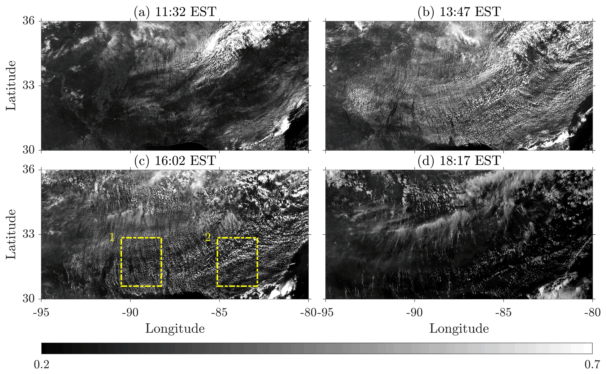
Figure 1 Corrected reflectance field of the diurnal cloud evolution as obtained from GOES-16 ABI's Red visible band (channel 2; 0.64 µm). Snapshots taken at 11:32 (a), 13:47 (b), 16:02 (c), and 18:17 EST (d). Dashed boxes in (c) represent two subdomains analyzed in Fig. 3.
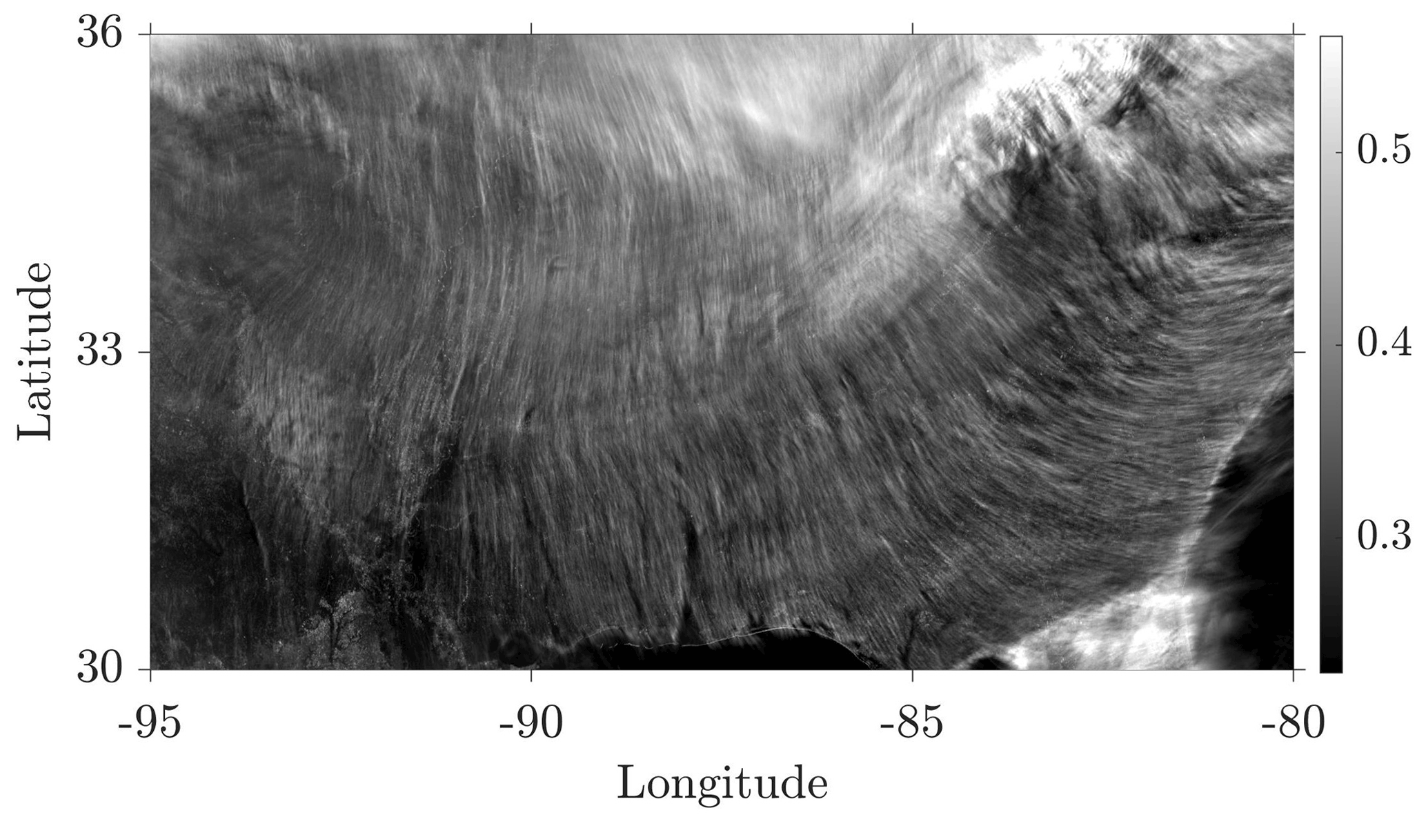
Figure 2 The time-averaged corrected reflectance field . Note the clear stripes in , marking the nearly stationary behavior of cloud streets along the mean CBL wind direction.
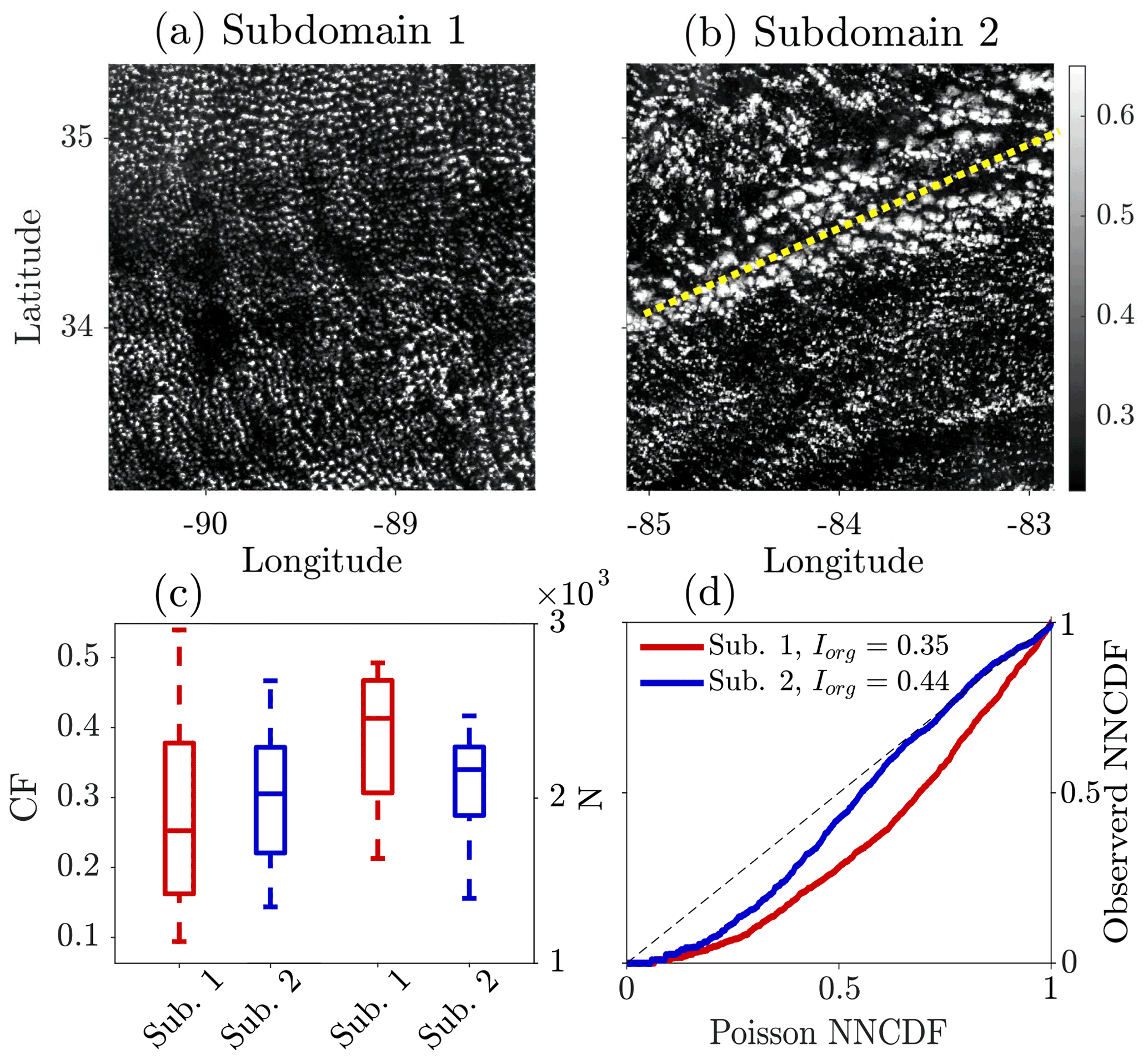
Figure 3 Snapshots of the two subdomains marked in Fig. 1c at 16:07 EST (a). Dashed yellow line in (b) shows the front of a GW. (c) Boxplots of the cloud fraction (CF) and the number of clouds (N) for subdomain-1 (red) and subdomain-2 (blue) between 15:02 and 18:02 EST. (d) Observed NNCDF against Poisson NNCDF for the two subdomains (color specification follows the one in c) at 16:07 EST. Diagonal dashed line shows a randomly distributed cloud field, while deviations above (below) the diagonal indicate a tendency toward clustering (regularity). The organization index (Iorg; Tompkins and Semie, 2017) of each subdomain is given in the top-left corner.
We focus on two subdomains (see boxes in Fig. 1c) and explore their organization (Fig. 3). While both of the subdomains exhibit a cloud street pattern, subdomain-2 also features the presence of GWs in the afternoon (indicated by a dashed line in Fig. 3b). GWs are frequently present in the atmosphere; they often occur over flat terrain and are ubiquitous over shallow Cu fields. In fact, the most intense and best organized GWs were reported over cloud streets (Kuettner et al., 1987). The latter, also known as convective GWs, are generated internally by the field with shallow Cu and/or the cloud streets acting as convective obstacles to the mean horizontal flow (Jaeckisch, 1972; Simpson, 1983; Melfi and Palm, 2012). Once excited, the GWs can act as a feedback mechanism to reorganize the convection, implying that the stable layer overlying the inversion plays an important role in determining the field's organization (Clark et al., 1986). In Fig. 3 we examine the effect of GWs, that may be challenging to observe with the naked eye, on the organization metrics of Sect. 2.2. The GWs evident in subdomain-2 result in larger-sized clouds, which is manifested in increased CF and decreased N during the afternoon (15:02–18:02 EST, Fig. 3c). By plotting the NNCDFs of the clouds' centroids in the two subdomains against the one of a randomly distributed cloud field given by the Poisson NNCDF (Weger et al., 1992) (Fig. 3d), we show that the two subdomains deviate from a random organization (Iorg<0.5, see Sect. 2.2) and exhibit a regular (grid-like) pattern, which is a high level of organization. This type of organization is typical for green Cu fields (Dror et al., 2020) and was reported in several continental areas, e.g., the Amazon basin (Da Silva et al., 2011; Heiblum et al., 2014), the US Southern Great Plains (Hinkelman and Evans, 2004), and northern Germany (Müller et al., 1985). However, due to the presence of GWs, the curve of the observed NNCDF of subdomain-2 lies closer to the diagonal and leans more towards clustered organization, resulting in a larger Iorg comparing to that of subdomain-1 (Iorg=0.44 and Iorg=0.35, respectively).
We note that even though we focus on the green Cu field, that covers most of the ROI during the day, there are other types of clouds that appear in the ROI: deeper orographic warm clouds in the upper-right corner (south edge of the Appalachian Mountains), mostly during noon to early afternoon; cirrus clouds at the north and central parts of the ROI, moving southward through the day (located above the Cu clouds); shallow early-morning clouds that dissipate at ∼11:30 EST further north to Florida; and deep convective clouds at the lower-right corner of the ROI that develop through the day (see the Supplement for more details regarding the cloud classification). However, the corrected reflectance field is clearly dominated by green Cu during the inspected time frame.
We further examine the cloud field's organization by conducting an EOF decomposition on the corrected reflectance images. Figure 4 shows the spectrum of the covariance matrix CX (see Sect. 2.3) and the field's key spatial features obtained by the EOF decomposition such as exhibited by the first three EOF modes; we refer to Figs. S5–S7 in the Supplement for the other EOF modes. The spectrum of the covariance matrix CX, shown in Fig. 4a, is composed of the eigenvalues which informs on the distribution of energy and on the separation/degeneracy of the EOF patterns. The corresponding PCs are shown in Fig. 5a. The leading mode (EOF1, 31.8 %) is nondegenerate (i.e., λ1 is well separated from the rest of the λk values; see Fig. 4a) and explains more than twice the variance than any other mode. Although the EOF decomposition is performed on the anomaly field (see Sect. 2.3), correlations between EOF1 and the mean field still remain (compare Figs. 2 and 4b), showing that these patterns constitute an important part of the field's variability. Thus, EOF1 displays the streets pattern of the green Cu field (Fig. 4b), while PC1 (Fig. 5a) shows a diurnal cycle manifestation whose magnitude peaks around local noon (in absolute value), coinciding with the evolution of green Cu. This is somehow not surprising as these clouds are closely linked to thermal convection; thus, their properties are tightly tied to the diurnal cycle of the surface fluxes (Stull, 1985; Zhu and Albrecht, 2002). They usually form around mid or late morning and dissipate before sunset (Zhu, 2003; Berg and Kassianov, 2008; Zhang and Klein, 2013). The second mode (EOF2, 14.8 %) (also nondegenerate) is mostly pronounced at the northeastern and southeastern parts of the ROI, displaying the general location of the orographic, shallow early-morning clouds and deep clouds marked in Fig. 4c as closed areas delimited by dash-dotted, dashed, and dotted curves, respectively (further evidence of these aspects is provided in the Supplement). PC2 is also dominated by a diurnal cycle but mostly pronounced in morning and late afternoon, i.e., before green Cu clouds emerge and after they disappear. The third mode (EOF3, 7.4 %) is marginally degenerate (depending on whether considering the error bars or not) and displays the structures of cirrus clouds at the northern part of the ROI (area enclosed by dotted curves in Fig. 4d). Furthermore, on the southeastern corner, we observe a blue–red contrast in patterns, which is indicative that EOF3 captures also some features of the deep-convective clouds more visible in EOF2; see also Fig. S5. An inspection of Fig. S5 reveals patterns that seem to propagate transversely to the cloud streets, as indicated by dashed lines therein.

Figure 4 (a) Spectrum (%) of the covariance matrix. Error bars calculation followed North et al. (1982). (b–d) The three leading EOF modes; units are arbitrary (the variance explained by each mode is noted at the title of each panel). Structures related to orographic, morning, and deep clouds are enclosed in dash-dotted, dashed, and dotted lines in (c), respectively. The structure related to cirrus clouds is enclosed in a dotted line in (d).
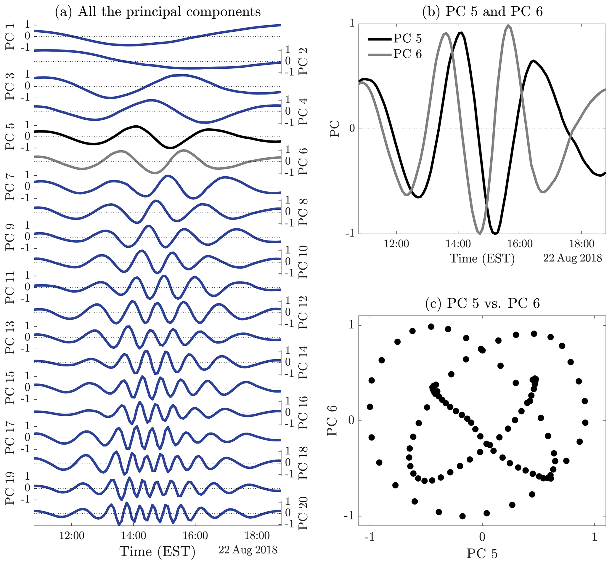
Figure 5Time series of the 20 PCs; PC5 and PC6 are marked in black and gray, respectively (a). Time series of PC5 and PC6 (b) and phase diagram of PC5 versus PC6 (c).
We turn now to a finer analysis of such patterns and EOF modes in general. The goal is to gain further understanding about the structures and scales exhibited by the EOFs, by analyzing the time variability of the corresponding PCs, providing the EOF's amplitude. Generally, in the case of a forward cascade of energy dissipation, a decaying energy distribution such as shown in Fig. 4a is thought to decay as a function of the spatial scale, with large-scale patterns that tend to capture most of the variance while evolving in time at a typical low frequency for the multivariate signal analyzed. But a word of caution must be mentioned here. This scenario of energy decay as a function of well-separated scales is indeed not always satisfied, and EOF modes exhibit sometimes a mixture of spatial scales, leading to various degrees of harmfulness for the analysis. Fortunately, for the dataset analyzed here, this phenomenon is not very pronounced. Indeed, only “an echo” of the cloud street patterns, mostly contained in EOF1, subsists in the higher modes (see Figs. 4c and d and S5), which benefits the analysis and interpretation.
As a result, by going down into the energy spectrum, the PCs move from low to higher frequencies. Low (respectively high) frequency translates to EOFs dominated by large-scale (respectively small-scale) patterns, and intermediate frequency to a mixture of these scales; see Figs. S5–S7. Grouping the PCs accordingly, the PC1–PC2 pair corresponds mainly to a low, diurnal-like time variability, PC3–PC9 all share an intermediate time variability, and PC10–PC20 are not only of higher frequency but also oscillate mainly during the time window over which PC1 peaks, i.e., when green Cu clouds are mostly pronounced. Among the PCs exhibiting an intermediate range of time variability (PC3–PC9), PC5 and PC6 are distinguished. The latter indeed reveal as forming an oscillatory pair, manifested by a phase shift between them in the time domain and by a nearly periodic behavior expressed by a nearly closed curve into the reduced state space spanned by EOF5 and EOF6; see Fig. 5. This pair of EOFs correspond to a 1.5 h near-period oscillation interpreted as the fingerprint of GWs traveling throughout the field (see e.g., Fig. 3b). GWs may propagate both horizontally and vertically above the inversion and were shown to have horizontal wavelengths of a few dozens of kilometers (Stull, 1976; Lane and Reeder, 2001; Lane, 2015) and to vertically extend throughout the whole troposphere (Clark et al., 1986; Kuettner et al., 1987; Hauf and Clark, 1989). Here we observe horizontally propagating GWs, with wavelength of ∼150 km as estimated from the stripe patterns in EOF5 and EOF6; see Text S1 and Fig. S5. A complementary analysis which consists of inspecting the time evolution of the field itself and its EOF reconstruction across a transection (red line in Fig. 6a and b) supports this interpretation as discussed next.
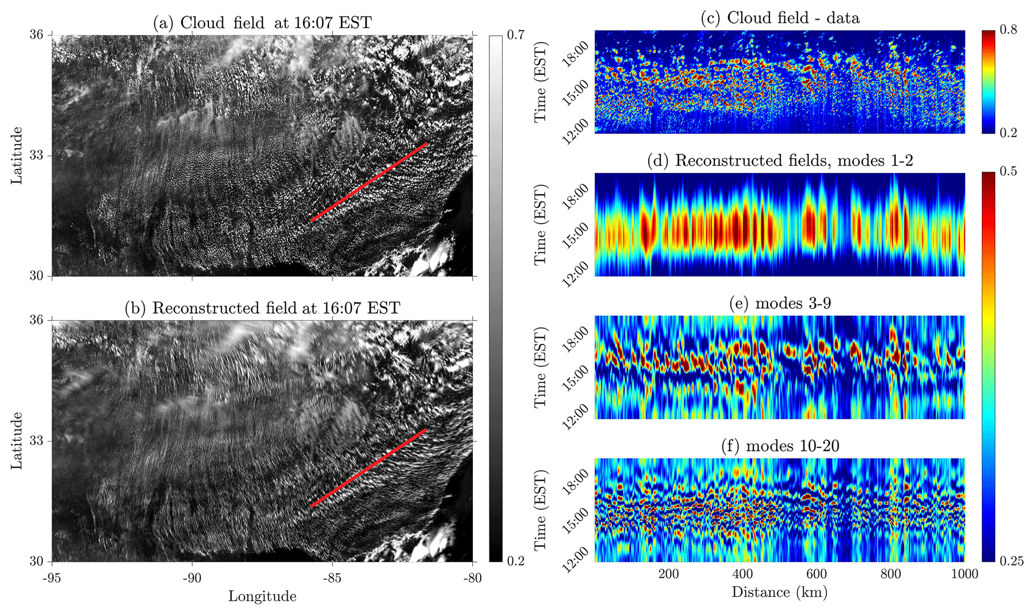
Figure 6Snapshot of the cloud field (a) and the field reconstructed using all 20 modes (b) at 16:07 EST. (c) Corrected reflectance as a function of time along the transaction marked in red in (a, b). Same as in (c) but for the field reconstructed from modes 1–2 (d), modes 3–9 (e), and modes 10–20 (f).
To better examine the presence of GWs in our green Cu field, we analyze the time evolution of the field across the transection orthogonal to the cloud streets, marked by the red line in Fig. 6a and b. The corresponding Hovmöller diagrams of the field's diurnal evolution are shown for the corrected reflectance data and for the reconstructed fields obtained by adding to the mean-field the sum of the PCs multiplied by their corresponding EOFs as in the right-hand side of Eq. (1) but for three groups of modes as follows: (i) the two leading ones (PCs 1–2 × EOFs 1–2), (ii) the intermediate ones (PCs 3–9 × EOFs 3–9), and (iii) the high-frequency ones (PCs 10–20 × EOFs 10–20). As mentioned above, the grouping of these modes is made according to their spatial degeneracy (Fig. 4a), on the one hand, and their temporal frequency (Fig. 5a), on the other. Recall that EOF modes 1–2 are both nondegenerate and feature a low, diurnal frequency. EOF modes 3–9 are marginally degenerate, still featuring substantial vertical change in Fig. 4a, and share an intermediate temporal frequency. EOF modes 10–20, however, are degenerate and belong to the flat part of the spectrum of the covariance matrix.
A snapshot (16:07 EST) of the field versus the reconstructed field (using the 20 EOF modes) is shown in Fig. 6a and b, respectively. The Hovmöller diagram obtained from the raw data is noisy (Fig. 6c), as it represents the superposition of several phenomena of different temporal and spatial scales. The diurnal cycle of the green Cu field is captured, with high reflectance values that start to appear in late morning time (∼11:00 EST) and disappear in the afternoon (∼18:00 EST). The prominent feature of the field's organization, i.e., the cloud streets, are only somewhat captured and appear as elongated discontinuous vertical features of high reflectance, composed of several reflectance blobs that represent the individual clouds that are advected through the transection. However, by decomposing the original, highly complex field, the diagrams of the reconstructed fields reveal a much clearer picture, and they allow us to extract important parameters of the field. The cloud streets in Fig. 6d appear continuous, more pronounced, and well-defined, and the spacing between them is also clearer (vertical features of low reflectance). Based on Fig. 6d, we estimate the street wavelengths as well as their aspect ratios (i.e., the street wavelengths divided by the CBL depth; Young et al., 2002; see Sect. S1 in the Supplement) to vary between 3–10.5 km. These values agree well with the range reported for continental cloud streets (Etling and Brown, 1993; Young et al., 2002; Da Silva et al., 2011). GWs, hardly observable in Fig. 6c, appear to be more distinguishable in Fig. 6e as nearly horizontal stripes of high reflectance. Within this representation, at least 2–3 waves appear during the day, with a dominant period of ∼1.5 h, in agreement with reported timescales about GWs (Tsuda, 2014; Nappo, 2013). Finally, EOFs 10–20 are able to capture individual clouds that form and dissipate as “pearls on a string” along the cloud streets throughout the day (see vertical oscillations along each cloud street in Fig. 6f). These higher-frequency modes also indicate that green Cu clouds in adjacent cloud streets, which may be distantly apart by tens to hundreds of kilometers, tend to form and dissipate in phase to form a rigid structure not only along the streets but also on the axis normal to the streets (see horizontal oscillations in Fig. 6f), shaping thus an immense, highly organized grid of clouds that lasts throughout the field's lifetime.
In this article, we proposed a new approach combining GOES-16 ABI's high-resolution corrected reflectance data, organization metrics, and an EOF analysis to investigate and characterize the mesoscale patterns obtained by a vast shallow Cu field over CONUS, during 22 August 2018. Organized shallow Cu clouds, referred to also as green Cu, start to form around late morning in response to daytime surface heating, reach their peak (in terms of cloud cover) from noon to early afternoon, and dissipate in the afternoon (Fig. 1). Cloud streets are evident throughout the whole domain, with their axis aligned along the mean advection direction, i.e., mostly in the north–south direction (northerlies). The cloud streets are sustained throughout the field's lifetime and maintain approximately fixed positions, which is apparent in the time-averaged field (Fig. 2). By focusing on two subdomains, we show that GWs, that are orthogonal to the cloud streets, travel through the field and affect the organization by clustering the clouds, thus making them larger and fewer, and that the clouds' organization deviates from randomness to a grid-like organization type (Fig. 3). The three leading modes of the EOF decomposition (Fig. 4b–d) reveal the field's most dominant spatial features, and the spectrum of the covariance matrix (Fig. 4a) shows the degeneracy of the leading EOF modes. The structure of the cloud streets, formed by the green Cu, is well-captured by the leading, nondegenerate EOF1, while (the nondegenerate) EOF2 relates to structures of other types of clouds that exist in the ROI, namely, orographic, shallow early-morning clouds, and deep clouds. EOF3 is marginally degenerate and therefore harder to relate to a specific physical phenomena; it contains a mixture of scales and structures, such as patterns of cirrus, deep clouds, and GWs. Over the time frame analyzed here, the time variability associated with the EOF modes is shown in Fig. 5a. The related PCs exhibit an organized set of timescales ranging from low via intermediate to high frequency, mostly expressed over the time window of the green Cu's diurnal cycle (∼11:00–18:00 EST). The different frequencies are related here to different spatial scales, such that lower frequencies correspond to EOF modes that are dominated by larger spatial structures. The intermediate frequencies are further explored by focusing on an oscillatory pair – PC5 and PC6. These two components demonstrate a nearly periodic 1.5 h oscillation with a phase shift, further indicating the existence of horizontally propagating GWs, which appear as stripes in the corresponding EOFs.
The full reconstruction of the field (using 20 modes) highly resembles the “real” field (Fig. 6a and b), even though the 20 modes explain only ∼65 % of the variance. By inspecting the field's time evolution through a transection along the GWs (orthogonal to the cloud streets), we identify features like the diurnal cycle and the cloud streets (Fig. 6c). However, the EOF decomposition allowed us to rebuild the field using subgroups of modes, thus separating between the scales (frequencies) and revealing different physical processes that interact to create the full complex patterns of the field. The reconstructed field time evolution (along the transection) presents the cloud streets, the GWs, and the individual clouds in a much clearer and cleaner manner (Fig. 6d–f, respectively), allowing us to extract important parameters like the cloud street wavelength, aspect ratio, and the GW period. Furthermore, the higher EOF modes reveal information regarding the organization of the field of a higher order nature. Not only are the green Cu clouds well organized as “pearls on a string” along the cloud streets, but the clouds are also showing coherent spatial organization in the axis transverse to the streets. Clouds forming on adjacent streets tend to form on the same phase and frequency, suggesting that a rigid grid structure forms not only in the spatial domain (as was shown in Fig. 3) but also in the temporal domain, on the timescale of the cloud field's lifetime, indicating a higher level of organization.
This study demonstrates that a standard decomposition of a shallow Cu field relying on EOFs, when performed on a well-prepared dataset, constitutes a useful tool for studying and characterizing the variety of patterns formed by the clouds within the field. The method allows, indeed, for disentangling the field's key organizational factors and for revealing hidden features which otherwise would be hard or even impossible to distinguish from a naked eye analysis of the underlying satellite dataset. Dimensionality reduction when performed with modes that convey the right dynamical information has proven its usefulness for the stochastic modeling and prediction of multiscale datasets in the recent years; see e.g. Kondrashov et al. (2018a), Kondrashov et al. (2018b), and Chekroun et al. (2011). In the case of the dataset analyzed here, the EOF modes provide such an efficient reduction that allows for the identification and capture of key dynamical features (cloud streets and GWs) and opens up, thus, new directions for data-driven stochastic modeling of shallow Cu fields.
All data used in this study are publicly available at https://www.avl.class.noaa.gov/ (GOES-16 ABI level 1b radiances, https://doi.org/10.7289/V5BV7DSR, GOES-R Calibration Working Group and GOES-R Series Program, 2017, GOES-16 ABI level 2 cloud top phase, https://doi.org/10.7289/V5NP22QW, GOES-R Algorithm Working Group and GOES-R Program Office, 2018 and cloud top height products, https://doi.org/10.7289/V5HX19ZQ, GOES-R Algorithm Working Group and GOES-R Program Office, 2018) and https://worldview.earthdata.nasa.gov/ (topography data, NASA JPL, 2013).
The video supplement related to this article is available online at https://doi.org/10.34933/wis.000007 (Koren, 2020).
The supplement related to this article is available online at: https://doi.org/10.5194/acp-21-12261-2021-supplement.
MDC conceived the presented idea. TD lead the analyses and MDC supported. TD, MDC, OA, and IK discussed the results and wrote the article. All co-authors provided critical feedback and helped shape the research, analysis, and article.
The authors declare that they have no conflict of interest.
Publisher's note: Copernicus Publications remains neutral with regard to jurisdictional claims in published maps and institutional affiliations.
This research received funding from the European Research Council (ERC) under the European Union's Horizon 2020 research and innovation program (grant agreement no. 810370). This research was partially supported by the Israeli Council for Higher Education (CHE) via the Weizmann Data Science Research Center.
The Climate Data Toolbox for MATLAB was used for the analysis (Greene et al., 2019).
This research has been supported by the Horizon 2020 (CloudCT (grant no. 810370)).
This paper was edited by Timothy Garrett and reviewed by two anonymous referees.
Agee, E. M., Chen, T., and Dowell, K.: A review of mesoscale cellular convection, B. Am. Meteorol. Soc., 54, 1004–1012, 1973. a
Atkinson, B. W. and Wu Zhang, J.: Mesoscale shallow convection in the atmosphere, Rev. Geophys., 34, 403–431, https://doi.org/10.1029/96RG02623, 1996. a
Berg, L. K. and Kassianov, E. I.: Temporal Variability of Fair-Weather Cumulus Statistics at the ACRF SGP Site, J. Climate, 21, 3344–3358, https://doi.org/10.1175/2007JCLI2266.1, 2008. a
Berg, L. K., Kassianov, E. I., Long, C. N., and Mills Jr., D. L.: Surface summertime radiative forcing by shallow cumuli at the Atmospheric Radiation Measurement Southern Great Plains site, J. Geophys. Res.-Atmos., 116, D01202, https://doi.org/10.1029/2010JD014593, 2011. a
Bony, S.: Marine boundary layer clouds at the heart of tropical cloud feedback uncertainties in climate models, Geophys. Res. Lett., 32, L20806, https://doi.org/10.1029/2005GL023851, 2005. a
Bony, S., Dufresne, J.-L., Le Treut, H., Morcrette, J.-J., and Senior, C.: On dynamic and thermodynamic components of cloud changes, Clim. Dynam., 22, 71–86, 2004. a
Boucher, O., Randall, D., Artaxo, P., Bretherton, C., Feingold, G., Forster, P., Kerminen, V.-M., Kondo, Y., Liao, H., Lohmann, U., Rasch, P., Satheesh, S. K., Sherwood, S., Stevens, B., and Zhang, X. Y.: Clouds and aerosols, in: Climate Change 2013: The Physical Science Basis. Contribution of Working Group I to the Fifth Assessment Report of the Intergovernmental Panel on Climate Change, edited by: Stocker, T. F., Qin, D., Plattner, G.-K., Tignor, M., Allen, S. K., Doschung, J., Nauels, A., Xia, Y., Bex, V., and Midgley, P. M.: Cambridge University Press, United Kingdom and New York USA, 571–657, https://doi.org/10.1017/CBO9781107415324.016, 2013. a
Brown, R. A.: Longitudinal instabilities and secondary flows in the planetary boundary layer: A review, Rev. Geophys., 18, 683–697, 1980. a, b
Chekroun, M. and Kondrashov, D.: Data-adaptive harmonic spectra and multilayer Stuart-Landau models, Chaos, 27, 093110, https://doi.org/10.1063/1.4989400, 2017. a
Chekroun, M. D., Kondrashov, D., and Ghil, M.: Predicting stochastic systems by noise sampling, and application to the El Niño-Southern Oscillation, P. Natl. Acad. Sci. USA, 108, 11766–11771, https://doi.org/10.1073/pnas.1015753108, 2011. a, b
Chen, C., Cane, M. A., Henderson, N., Lee, D. E., Chapman, D., Kondrashov, D., and Chekroun, M.: Diversity, Nonlinearity, Seasonality, and Memory Effect in ENSO Simulation and Prediction Using Empirical Model Reduction, J. Climate, 29, 1809–1830, 2016. a
Cheng, X., Nitsche, G., and Wallace, J. M.: Robustness of low-frequency circulation patterns derived from EOF and rotated EOF analyses, J. Climate, 8, 1709–1713, 1995. a
Clark, T. L., Hauf, T., and Kuettner, J. P.: Convectively forced internal gravity waves: Results from two-dimensional numerical experiments, Q. J. Roy. Meteor. Soc., 112, 899–925, 1986. a, b
Da Silva, R. R., Gandu, A. W., Sá, L. D., and Dias, M. A. S.: Cloud streets and land–water interactions in the Amazon, Biogeochemistry, 105, 201–211, 2011. a, b
Dagan, G., Koren, I., Kostinski, A., and Altaratz, O.: Organization and oscillations in simulated shallow convective clouds, J. Adv. Model. Earth Sy., 10, 2287–2299, 2018. a
DelSole, T. and Tippett, M. K.: Average predictability time. Part I: theory, J. Atmos. Sci., 66, 1172–1187, 2009. a
Dror, T., Koren, I., Altaratz, O., and Heiblum, R. H.: On the Abundance and Common Properties of Continental, Organized Shallow (Green) Clouds, IEEE T. Geosci. Remote, 59, 4570–4578, 2020. a, b, c, d
Etling, D. and Brown, R.: Roll vortices in the planetary boundary layer: A review, Bound.-Lay. Meteorol., 65, 215–248, 1993. a, b
Fukuoka, A.: The central meteorological observatory, a study on 10-day forecast (a synthetic report), Geophysical Magazine, 22, 177–208, 1951. a
GOES-R Algorithm Working Group and GOES-R Program Office: NOAA GOES-R Series Advanced Baseline Imager (ABI) Level 2 Cloud Top Phase (ACTP), CONUS subset, NOAA National Centers for Environmental Information [data set], https://doi.org/10.7289/V5NP22QW, 2018a. a, b
GOES-R Algorithm Working Group and GOES-R Series Program Office: NOAA GOES-R Series Advanced Baseline Imager (ABI) Level 2 Cloud Top Height (ACHA), CONUS subset, NOAA National Centers for Environmental Information [data set], https://doi.org/10.7289/V5HX19ZQ, 2018.
GOES-R Calibration Working Group and GOES-R Series Program: NOAA GOES-R Series Advanced Baseline Imager (ABI) Level 1b Radiances, CONUS subset, NOAA National Centers for Environmental Information [data set], https://doi.org/10.7289/V5BV7DSR, 2017. a
Greene, C. A., Thirumalai, K., Kearney, K. A., Delgado, J. M., Schwanghart, W., Wolfenbarger, N. S., Thyng, K. M., Gwyther, D. E., Gardner, A. S., and Blankenship, D. D.: The climate data toolbox for MATLAB, Geochem. Geophy. Geosy., 20, 3774–3781, https://doi.org/10.1029/2019GC008392, 2019. a
Groth, A. and Ghil, M.: Multivariate singular spectrum analysis and the road to phase synchronization, Phys. Rev. E, 84, 036206, https://doi.org/10.1103/PhysRevE.84.036206, 2011. a
Hannachi, A., Jolliffe, I., Stephenson, D., and Trendafilov, N.: In search of simple structures in climate: simplifying EOFs, Int. J. Climatol., 26, 7–28, 2006. a
Hauf, T. and Clark, T. L.: Three-dimensional numerical experiments on convectively forced internal gravity waves, Q. J. Roy. Meteor. Soc., 115, 309–333, 1989. a
Heiblum, R. H., Koren, I., and Feingold, G.: On the link between Amazonian forest properties and shallow cumulus cloud fields, Atmos. Chem. Phys., 14, 6063–6074, https://doi.org/10.5194/acp-14-6063-2014, 2014. a
Heus, T. and Seifert, A.: Automated tracking of shallow cumulus clouds in large domain, long duration large eddy simulations, Geosci. Model Dev., 6, 1261–1273, https://doi.org/10.5194/gmd-6-1261-2013, 2013. a
Hinkelman, L. and Evans, K.: Anisotropy in Broken Cloud Fields Over Oklahoma from Landsat Data, Fourteenth ARM Science Team Meeting Proceedings, Albuquerque, New Mexico, 22–26 March 2004. a
Horel, J. D.: A rotated principal component analysis of the interannual variability of the Northern Hemisphere 500 mb height field, Mon. Weather Rev., 109, 2080–2092, 1981. a
Jaeckisch, H.: Synoptic conditions of wave formation above convective streets, OSTIV Publications, Braunschweig, Germany, 12, 1972. a
Jakub, F. and Mayer, B.: The role of 1-D and 3-D radiative heating in the organization of shallow cumulus convection and the formation of cloud streets, Atmos. Chem. Phys., 17, 13317–13327, https://doi.org/10.5194/acp-17-13317-2017, 2017. a
Jolliffe, I.: Principal Component Analysis, 2nd Edn., Springer, New York, 2002. a
Kawamura, R.: A rotated EOF analysis of global sea surface temperature variability with interannual and interdecadal scales, J. Phys. Oceanogr., 24, 707–715, 1994. a
Klitch, M. A., Weaver, J. F., Kelly, F. P., and Vonder Haar, T. H.: Convective cloud climatologies constructed from satellite imagery, Mon. Weather Rev., 113, 326–337, 1985. a
Kondrashov, D., Chekroun, M., and Berloff, P.: Multiscale Stuart-Landau emulators: Application to wind-driven ocean gyres, Fluids, 3, 21, https://doi.org/10.3390/fluids3010021, 2018a. a
Kondrashov, D., Chekroun, M. D., Yuan, X., and Ghil, M.: Data-adaptive harmonic decomposition and stochastic modeling of Arctic sea ice, in: Advances in Nonlinear Geosciences, edited by: A. Tsonis, Springer, Cham, Switzerland, 179–205, 2018b. a
Koren, I.: Data from: Deciphering Organization of GOES–16 Green Cumulus, through the EOF lens, The Weizmann Institute of Science [data set], https://doi.org/10.34933/wis.000007, 2020. a
Kuettner, J. P., Hildebrand, P. A., and Clark, T. L.: Convection waves: Observations of gravity wave systems over convectively active boundary layers, Q. J. Roy. Meteor. Soc., 113, 445–467, 1987. a, b
Lane, T. P.: Convectively generated gravity waves, in: Encyclopedia of Atmospheric Sciences, 2nd Edn., Elsevier, Amsterdam, Netherland, 171–179, 2015. a
Lane, T. P. and Reeder, M. J.: Convectively generated gravity waves and their effect on the cloud environment, J. Atmos. Sci., 58, 2427–2440, 2001. a
Lorenz, E. N.: Empirical orthogonal functions and statistical weather prediction, Scientific Report no. 1, Statistical Forecasting Project, Massachusetts Institute of Technology, Department of Meteorology Cambridge, 1956. a
Melfi, S. and Palm, S. P.: Estimating the orientation and spacing of midlatitude linear convective boundary layer features: Cloud streets, J. Atmos. Sci., 69, 352–364, 2012. a
Messié, M. and Chavez, F.: Global modes of sea surface temperature variability in relation to regional climate indices, J. Climate, 24, 4314–4331, 2011. a
Mestas-Nuñez, A. M. and Enfield, D. B.: Rotated global modes of non-ENSO sea surface temperature variability, J. Climate, 12, 2734–2746, 1999. a
Monahan, A. H., Fyfe, J. C., Ambaum, M. H., Stephenson, D. B., and North, G. R.: Empirical orthogonal functions: The medium is the message, J. Climate, 22, 6501–6514, 2009. a
Müller, D., Etling, D., Kottmeier, C., and Roth, R.: On the occurrence of cloud streets over northern Germany, Q. J. Roy. Meteor. Soc., 111, 761–772, 1985. a
Nair, U., Weger, R., Kuo, K., and Welch, R.: Clustering, randomness, and regularity in cloud fields: 5. The nature of regular cumulus cloud fields, J. Geophys. Res.-Atmos., 103, 11363–11380, 1998. a
Nappo, C. J.: An Introduction to Atmospheric Gravity Waves, Academic press, Cambridge, Massachusetts, USA, 2013. a
NASA JPL: NASA Shuttle Radar Topography Mission Global 1 arc second, SRTMGL1 v003, NASA EOSDIS Land Processes DAAC [data set], https://doi.org/10.5067/MEaSUREs/SRTM/SRTMGL1.003, 2013. a
Norris, J. R.: Low cloud type over the ocean from surface observations. Part II: Geographical and seasonal variations, J. Climate, 11, 383–403, 1998. a
North, G. R., Bell, T. L., Cahalan, R. F., and Moeng, F. J.: Sampling errors in the estimation of empirical orthogonal functions, Mon. Weather Rev., 110, 699–706, 1982. a, b
Nuijens, L. and Siebesma, A. P.: Boundary layer clouds and convection over subtropical oceans in our current and in a warmer climate, Current Climate Change Reports, 5, 80–94, 2019. a
Penland, C. and Magorian, T.: Prediction of Niño 3 sea surface temperatures using linear inverse modeling, J. Climate, 6, 1067–1076, 1993. a
Penland, C. and Sardeshmukh, P. D.: The optimal growth of tropical sea surface temperature anomalies, J. Climate, 8, 1999–2024, 1995. a
Rabin, R. M. and Martin, D. W.: Satellite observations of shallow cumulus coverage over the central United States: An exploration of land use impact on cloud cover, J. Geophys. Res.-Atmos., 101, 7149–7155, 1996. a
Ray, D. K., Nair, U. S., Welch, R. M., Han, Q., Zeng, J., Su, W., Kikuchi, T., and Lyons, T. J.: Effects of land use in Southwest Australia: 1. Observations of cumulus cloudiness and energy fluxes, J. Geophys. Res.-Atmos., 108, 4414, https://doi.org/10.1029/2002JD002654, 2003. a
Richman, M. B.: Obliquely rotated principal components: An improved meteorological map typing technique?, J. Appl. Meteorol., 20, 1145–1159, 1981. a
Richman, M. B.: Rotation of principal components, J. Climatol., 6, 293–335, 1986. a
Roundy, P. E. and Schreck III, C. J.: A combined wave-number–frequency and time-extended EOF approach for tracking the progress of modes of large-scale organized tropical convection, Q. J. Roy. Meteor. Soc., 135, 161–173, 2009. a
Schmit, T., Gunshor, M., Fu, G., Rink, T., Bah, K., and Wolf, W.: GOES-R Advanced Baseline Imager (ABI) Algorithm Theoretical Basis Document for: Cloud and Moisture Imagery Product (CMIP), University of Wisconsin–Madison, Madison, Wisconsin, USA, 2010. a
Schmit, T. J., Griffith, P., Gunshor, M. M., Daniels, J. M., Goodman, S. J., and Lebair, W. J.: A closer look at the ABI on the GOES-R series, B. Am. Meteorol. Soc., 98, 681–698, 2017. a, b
Seifert, A. and Heus, T.: Large-eddy simulation of organized precipitating trade wind cumulus clouds, Atmos. Chem. Phys., 13, 5631–5645, https://doi.org/10.5194/acp-13-5631-2013, 2013. a, b
Simpson, J.: Cumulus clouds: Early aircraft observations and entrainment hypotheses, in: Mesoscale Meteorology – Theories, Observations and Models, Springer, Berlin/Heidelberg, Germany, 355–373, 1983. a
Stevens, B., Bony, S., Brogniez, H., Hentgen, L., Hohenegger, C., Kiemle, C., L'Ecuyer, T., Naumann, A., Schulz, H., Siebesma, P., Vial, J., Winker, D., and Zuidema, P.: Sugar, gravel, fish and flowers: Mesoscale cloud patterns in the trade winds, Q. J. Roy. Meteor. Soc., 146, 1–12, 2019. a
Stull, R. B.: Internal gravity waves generated by penetrative convection, J. Atmos. Sci., 33, 1279–1286, 1976. a
Stull, R. B.: A Fair-Weather Cumulus Cloud Classification Scheme for Mixed-Layer Studies, J. Clim. Appl. Meteorol., 24, 49–56, 1985. a, b
Thompson, D. W. and Wallace, J. M.: The Arctic Oscillation signature in the wintertime geopotential height and temperature fields, Geophys. Res. Lett., 25, 1297–1300, 1998. a
Tobin, I., Bony, S., and Roca, R.: Observational evidence for relationships between the degree of aggregation of deep convection, water vapor, surface fluxes, and radiation, J. Climate, 25, 6885–6904, 2012. a
Tompkins, A. M. and Semie, A. G.: Organization of tropical convection in low vertical wind shears: Role of updraft entrainment, J. Adv. Model. Earth Sy., 9, 1046–1068, 2017. a, b
Tsuda, T.: Characteristics of atmospheric gravity waves observed using the MU (Middle and Upper atmosphere) radar and GPS (Global Positioning System) radio occultation, P. Jpn. Acad. B-Phys., 90, 12–27, 2014. a
Turner, D. D., Vogelmann, A. M., Austin, R. T., Barnard, J. C., Cady-Pereira, K., Chiu, J. C., Clough, S. A., Flynn, C., Khaiyer, M. M., Liljegren, J., Johnson, K., Lin, B., Long, C., Marshak, A., Matrosov, S. Y., McFarlane, S. A., Miller, M., Min, Q., Minimis, P., O'Hirok, W., Wang, Z., and Wiscombe, W.: Thin liquid water clouds: their importance and our challenge, B. Am. Meteorol. Soc., 88, 177–190, https://doi.org/10.1175/BAMS-88-2-177, 2007. a
Vial, J., Bony, S., Stevens, B., and Vogel, R.: Mechanisms and model diversity of trade-wind shallow cumulus cloud feedbacks: a review, in: Shallow Clouds, Water Vapor, Circulation, and Climate Sensitivity, Springer, NYC, NY, USA, 159–181, 2017. a
Weare, B. C. and Nasstrom, J. S.: Examples of extended empirical orthogonal function analyses, Mon. Weather Rev., 110, 481–485, 1982. a
Webb, M. J., Senior, C., Sexton, D., Ingram, W., Williams, K., Ringer, M., McAvaney, B., Colman, R., Soden, B. J., Gudgel, R., Knutson, T., Emori, S., Ogura, T., Tsushima, Y., Andronova, N., Li, B., Musat, I., Bony, S., and Taylor, K. E.: On the contribution of local feedback mechanisms to the range of climate sensitivity in two GCM ensembles, Clim. Dynam., 27, 17–38, 2006. a
Weckwerth, T. M., Wilson, J. W., Wakimoto, R. M., and Crook, N. A.: Horizontal convective rolls: Determining the environmental conditions supporting their existence and characteristics, Mon. Weather Rev., 125, 505–526, 1997. a
Weger, R., Lee, J., Zhu, T., and Welch, R.: Clustering, randomness and regularity in cloud fields: 1. Theoretical considerations, J. Geophys. Res.-Atmos., 97, 20519–20536, 1992. a, b
Wing, A. A. and Emanuel, K. A.: Physical mechanisms controlling self-aggregation of convection in idealized numerical modeling simulations, J. Adv. Model. Earth Sy., 6, 59–74, 2014. a
Xue, H., Feingold, G., and Stevens, B.: Aerosol effects on clouds, precipitation, and the organization of shallow cumulus convection, J. Atmos. Sci., 65, 392–406, 2008. a
Young, G. S., Kristovich, D. A., Hjelmfelt, M. R., and Foster, R. C.: Rolls, streets, waves, and more: A review of quasi-two-dimensional structures in the atmospheric boundary layer, B. Am. Meteorol. Soc., 83, 997–1002, 2002. a, b
Zelinka, M. D., Myers, T. A., McCoy, D. T., Po-Chedley, S., Caldwell, P. M., Ceppi, P., Klein, S. A., and Taylor, K. E.: Causes of higher climate sensitivity in CMIP6 models, Geophys. Res. Lett., 47, e2019GL085782, https://doi.org/10.1029/2019GL085782, 2020. a
Zhang, Y. and Klein, S. A.: Factors Controlling the Vertical Extent of Fair-Weather Shallow Cumulus Clouds over Land: Investigation of Diurnal-Cycle Observations Collected at the ARM Southern Great Plains Site, J. Atmos. Sci., 70, 1297–1315, https://doi.org/10.1175/JAS-D-12-0131.1, 2013. a, b
Zhu, P.: Large eddy simulations of continental shallow cumulus convection, J. Geophys. Res., 108, 4453, https://doi.org/10.1029/2002JD003119, 2003. a
Zhu, P. and Albrecht, B.: A theoretical and observational analysis on the formation of fair-weather cumuli, J. Atmos. Sci., 59, 1983–2005, 2002. a
Zhu, T., Lee, J., Weger, R., and Welch, R.: Clustering, randomness, and regularity in cloud fields: 2. Cumulus cloud fields, J. Geophys. Res.-Atmos., 97, 20537–20558, 1992. a