The reduction in C₂H₆ from 2015 to 2020 over Hefei, eastern China, points to air quality improvement in China

Ethane (C₂H₆) is an important greenhouse gas and plays a significant role in tropospheric chemistry and climate change. This study first presents and then quantifies the variability, sources, and transport of C₂H₆ over densely populated and highly industrialized eastern China using ground-based high-resolution Fourier transform infrared (FTIR) remote sensing along with atmospheric modeling techniques. We obtained a retrieval error of 6.21 ± 1.2 (1σ)% and degrees of freedom (DOFS) of 1.47 ± 0.2 (1σ) in the retrieval of C₂H₆ tropospheric column-averaged dry-air mole fraction (troDMF) over Hefei, eastern China (32^∘ N, 117^∘ E; 30 $\mathrm{m}\mathrm{a}.\mathrm{s}.\mathrm{l}.$). The observed C₂H₆ troDMF reached a minimum monthly mean value of 0.36 ± 0.26 ppbv in July and a maximum monthly mean value of 1.76 ± 0.35 ppbv in December, and showed a negative change rate of −2.60 ± 1.34 % yr⁻¹ from 2015 to 2020. The dependencies of C₂H₆ troDMF on meteorological and emission factors were analyzed using generalized additive models (GAMs). Generally, both meteorological and emission factors have positive influences on C₂H₆ troDMF in the cold season (December–January–February/March–April–May, DJF/MAM) and negative influences on C₂H₆ troDMF in the warm season (June–July–August/September–October–November, JJA/SON). GEOS-Chem chemical model simulation captured the observed C₂H₆ troDMF variability and was, thus, used for source attribution. GEOS-Chem model sensitivity simulations concluded that the anthropogenic emissions (fossil fuel plus biofuel emissions) and the natural emissions (biomass burning plus biogenic emissions) accounted for 48.1 % and 39.7 % of C₂H₆ troDMF variability over Hefei, respectively. The observed C₂H₆ troDMF variability mainly results from the emissions within China (74.1 %), where central, eastern, and northern China dominated the contribution (57.6 %). Seasonal variability in C₂H₆ transport inflow and outflow over the observation site is largely related to the midlatitude westerlies and the Asian monsoon system. Reduction in C₂H₆ abundance from 2015 to 2020 mainly results from the decrease in local and transported C₂H₆ emissions, which points to air quality improvement in China in recent years.

1 Introduction

Ethane (C₂H₆) is an important greenhouse gas and one of the most abundant volatile organic compounds (VOCs) in the atmosphere (Abad et al., 2011; Singh et al., 2001; Steinfeld, 1998). Although C₂H₆ is much less abundant than methane (CH₄) and also less efficient relative to mass, it plays a significant role in tropospheric chemistry and climate change (Tzompa-Sosa et al., 2017). In the presence of nitrogen oxides (NO_x = NO + NO₂), C₂H₆ oxidation can enhance tropospheric ozone (O₃) generation, which shows a positive radiative influence on climate (Sun et al., 2018a) and threatens crop yields (Sun et al., 2018a; Van Dingenen et al., 2009) and human health (Sun et al., 2018a; Tzompa-Sosa et al., 2017). In addition, as a major source of acetaldehyde (CH₃CHO), C₂H₆ has a great impact on the production of peroxyacetyl nitrate (PAN) which is a key reservoir species of NO_x (Fischer et al., 2014). The main sink of tropospheric C₂H₆ is predominantly destruction via reaction with the hydroxyl radical (OH) (Xiao et al., 2008), which determines the residence time of most tropospheric species (Steinfeld, 1998). As a result, tropospheric C₂H₆ can decrease the atmospheric oxidative capacity and indirectly impact the climate by extending the CH₄ lifetime (Monks et al., 2018; Taylor et al., 2020). Atmospheric C₂H₆ has a relatively long residence time of a few months (Franco et al., 2016), allowing it to undergo intercontinental transport. As a result, observations of C₂H₆ can be assimilated into a chemical transport model to estimate nonlocal emissions and air quality, and provide valuable insights into model biases of C₂H₆ simulations (Tzompa-Sosa et al., 2017).

On a global scale, the main sources of C₂H₆ are leakage from production, processing, and transport of natural gas (62 %), and biofuel combustion (20 %) and biomass burning emission (18 %) largely occurred in the Northern Hemisphere (NH) (Franco et al., 2016; Xiao et al., 2008). Additional minor sources of C₂H₆ are from biogenic and oceanic sources. However, on a regional scale, the proportion of each C₂H₆ source may show large differences. The natural gas leakage contribution can reach 80 % of C₂H₆ emissions in regions with active oil and natural gas production (Gilman et al., 2013), where C₂H₆ emissions are highly correlated with CH₄ emissions. In such regions, C₂H₆ can be applied as a tracer for the separation of fossil fuel CH₄ emissions from multiple methane (CH₄) sources (e.g., oil and gas, cows, wetlands, and rice yield) (McKain et al., 2015; Roscioli et al., 2015). The C₂H₆ abundance in the Southern Hemisphere (SH) is much lower than that in the NH, as the anthropogenic C₂H₆ sources are low in the SH and the residence time of C₂H₆ is shorter than the interhemispheric exchange rate. Many studies have concluded that C₂H₆ in the SH is primarily emitted from biomass burning and is closely correlated with CO and HCN emissions (Notholt et al., 2000; Rinsland et al., 2002; Vigouroux et al., 2012; Zeng et al., 2012).

C₂H₆ is one of the target gases of a global ground-based Fourier transform infrared spectroscopy (FTIR) network, namely the infrared working group (IRWG) of the Network for Detection of Atmospheric Composition Change (NDACC) (De Mazière et al., 2018). FTIR time series of C₂H₆ with different time periods have been reported at many stations for the validation of satellite data or chemical model simulation (Abad et al., 2011; Franco et al., 2015, 2016; Glatthor et al., 2009) or for the evaluation of local air quality and air pollutant transport caused by anthropogenic emission and biomass burning (Angelbratt et al., 2011; Lutsch et al., 2016, 2019; Nagahama and Suzuki, 2007; Rinsland et al., 2002; Simpson et al., 2012; Viatte et al., 2015, 2014; Vigouroux et al., 2012; Zeng et al., 2012; Zhao et al., 2002). Several FTIR sites have observed the decrease in C₂H₆ over the 1990–2010 period and have characterized consistent interannual trends in the −1 to −2.7 % yr⁻¹ range (Franco et al., 2015, 2016; Simpson et al., 2012; Zeng et al., 2012). This declining trend has been largely attributed to the reduction in global fugitive emissions (Franco et al., 2015; Simpson et al., 2012). Recently, several studies concluded that the long-term decline in C₂H₆ in the NH reversed from 2009 onwards (Franco et al., 2015, 2016). Using ground-based FTIR C₂H₆ total columns derived at five selected NDACC sites, Franco et al. (2016) characterized the C₂H₆ evolution from 2009 to 2015 and determined growth rates of ∼ 3 % yr⁻¹ at remote sites and of ∼ 5 % yr⁻¹ at midlatitudes. This change is mainly attributed to the exploitation of shale gas and tight oil reservoirs in North America (Franco et al., 2016; Helmig et al., 2016).

The NDACC network has been operating for almost 3 decades around the globe (De Maziere et al., 2018; Sun et al., 2018a). However, most instruments are located in Europe and Northern America, the number of observation sites in the rest parts of world remains sparse, and there is only one qualified observations site in China, i.e., the Hefei site (32^∘ N, 117^∘ E; 30 $\mathrm{m}\mathrm{a}.\mathrm{s}.\mathrm{l}.$), located in a densely populated and highly industrialized area in eastern China (Sun et al., 2018a). The Hefei site is not yet affiliated with the NDACC network, but its observation routine has followed the NDACC standard convention since 2015 (Sun et al., 2018a). As the consequence of a series of actions for emission control, air pollution over China in recent years has been significantly decreased (Zhang et al., 2019; Zheng et al., 2018). However, the atmospheric pollution over densely populated and highly industrialized eastern China is still severe (Zhang et al., 2019; Zheng et al., 2018). The complexity, extension, and severity of the atmospheric pollution in eastern China are still unrivaled compared with the rest of world (Lu et al., 2018; Zheng et al., 2018). FTIR observations at Hefei have been used extensively for the evaluation of satellite data (Tian et al., 2018; Wang et al., 2017), chemical model simulation (Tian et al., 2018; Yin et al., 2020, 2019), local air quality (Shan et al., 2019; Sun et al., 2018a), and the transport of air pollutants caused by anthropogenic and biomass burning emissions (Sun et al., 2018a, 2000; Y. Sun et al., 2021).

In this study, we first present and then quantify the variability, sources, and transport of C₂H₆ over densely populated and highly industrialized eastern China using FTIR observation, GEOS-Chem model simulation, and the analysis of the meteorological fields. The seasonality and interannual variability of C₂H₆ over Hefei, eastern China, from 2015 to 2020 are investigated. The dependencies of C₂H₆ on meteorological and co-emitted gases (hereafter emission factors) are analyzed using generalized additive models (GAMs) (Wood and Simon, 2004). The ground-based FTIR C₂H₆ time series are, for the first time, applied to evaluate the GEOS-Chem model with respect to the simulation of C₂H₆ for specific polluted regions over eastern China. Furthermore, we run a series of GEOS-Chem sensitivity simulations to quantify the relative contributions of various source categories and regions to the observed C₂H₆ variability. The three-dimensional (3D) transport inflow and outflow pathways of C₂H₆ over the observation site are finally determined by the GEOS-Chem sensitivity simulations and the analysis of the meteorological fields. This study can not only enhance the understanding of regional emission, transport, and air clean actions over eastern China but can also contribute to form new reliable remote sensing data in this sparsely monitored region for climate change research.

The next section describes the retrieval of the FTIR tropospheric column-averaged dry-air mole fraction (troDMF) of C₂H₆, the configuration of GEOS-Chem model simulation, and the GAMs regression approach. Section 3 reports the variability of C₂H₆ troDMF and a comparison with the GEOS-Chem simulation. Section 4 reports the GAMs regression results and the interpretation. Section 5 reports the results for source attribution using a GEOS-Chem sensitivity simulation and the analysis of the meteorological fields. We conclude the study in Sect. 6.

2 Methods and data

2.1 C₂H₆ troDMF retrieval

The C₂H₆ troDMF time series were calculated using direct solar absorption spectra saved with a FTIR spectrometer in operation at Hefei, eastern China (Sun et al., 2018a; Tian et al., 2018). A site description and instrumentation can be found in Sun et al. (2018a). Briefly, the FTIR observatory includes a high-resolution FTIR spectrometer (IFS125HR, Bruker) and a solar tracker (Solar Tracker A547, Bruker). The instrument has been operating continuously since its installation; however, short data gaps of up to 8 months have occurred due to a scanner problem between November 2016 and July 2017. This FTIR observatory alternately saved near-infrared (NIR) and middle-infrared (MIR) solar spectra in routine observations, with spectral ranges from 4000 to 11 000 cm⁻¹ and from 500 to 8500 cm⁻¹, respectively (Tian et al., 2018). The NIR and MIR spectra are saved with different spectral resolutions, but both of them can be used to retrieve total columns and volume mixing ratio (VMR) profiles of a variety of trace gases in the atmosphere. The MIR spectra used in the present work are saved with a spectral resolution of 0.005 cm⁻¹ following the requirements of the NDACC standard convention (http://www.ndacc.org/, last accessed on 27 December 2020). The FTIR instrument is equipped with a KBr beam splitter, a filter centered at 2800 cm⁻¹, and an InSb detector for C₂H₆ measurements. The number of C₂H₆ measurements on each measurement day varied from 1 to 17 with an average of 6. In total, there were 743 d of qualified measurements between 2015 and 2020.

In this study, the VMR profile of C₂H₆ was first retrieved using the SFIT4 algorithm, updated from SFIT2 (Pougatchev et al., 1995), and implementing the optimal estimation method (Rodgers, 2000). The C₂H₆ troDMF was then calculated by taking a weighting average of the C₂H₆ VMR profile and the air mass using a fixed tropospheric altitude. The C₂H₆ VMR profile was retrieved in a broad window of 2976–2978 cm⁻¹. The VMR profiles of CH₄ and H₂O and column of O₃ were also retrieved along with the C₂H₆ VMR profile for minimizing the atmospheric absorption interference. Spectroscopic absorption parameters of all gases are based on the atm16 line list from the compilation of Geoffrey Toon (Y. Sun et al., 2021). The a priori vertical profiles of temperature, H₂O, and pressure were interpolated from the National Centers for Environmental Protection (NCEP) reanalysis data, and the a priori vertical profiles of other gases were from the statistical averages of the Whole Atmosphere Community Climate Model version 6 (WACCM) simulations from 1980 to 2020. The diagonal elements of the a priori covariance matrices S_a and the measurement noise covariance matrices S_ε were set to the standard deviation (SD) of the WACCM simulations and the inverse square of the signal-to-noise ratio (SNR) of each spectrum, respectively (Franco et al., 2015). The non-diagonal elements of both S_a and S_ε were set to zero. The instrument line shape (ILS) of the FTIR instrument deduced from optical path alignment diagnosis with a low-pressure HBr cell was adopted in the retrieval (Hase, 2012; Sun et al., 2018b).

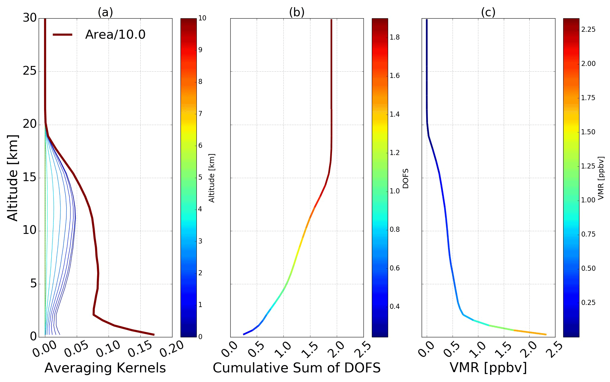
Figure 1 (a) Averaging kernels and their area scaled by a factor of 0.1, (b) cumulative sum of degrees of freedom for signal (DOFS), and (c) volume mixing ratio (VMR) profile of a randomly selected C₂H₆ retrieval over Hefei, eastern China.

For each retrieval, the averaging kernels reflect the sensitivity of the retrieved profile to the real profile. The area of the averaging kernels at a specific height is calculated as the sum of the elements of the corresponding averaging kernels (Pougatchev et al., 1995). It represents the fraction of the retrieval at that height that comes from the measurement rather than from the a priori information (Rodgers, 2000). A value close to unity at a specific height indicates that the retrieved profile at that height is nearly independent of the a priori profile and is, thus, from the measurement. The trace of the averaging kernel matrix is defined as degrees of freedom for signal (DOFS) and it quantifies the number of independent pieces of information in the retrieved profile. Figure 1 shows the averaging kernels as well as their area, cumulative sum of DOFS, and VMR profile of a randomly selected at Hefei. Ground-based FTIR C₂H₆ observations at Hefei have a sensitivity of larger than 0.7 from ground to about 10 km altitude, indicating that the retrievals are mainly sensitive to the troposphere. This also means that more than 70 % of the retrieved profile information below 10 km comes from the measurement, or in other words, that the a priori signal impacts the retrieval by less than 30 % (Fig. 1a). The typical DOFS obtained at Hefei over the total atmosphere for C₂H₆ is 1.69 ± 0.29 (1σ), meaning that we can roughly provide two pieces of information on the vertical profile (Fig. 1b). The shape of the retrieved profile is heavily weighted toward the lower troposphere. As shown in Fig. 1c, the C₂H₆ concentration decreased by 72.7 % with an increase in the height from surface to 2 km and kept decreasing slowly in the remaining part of the atmosphere until it approached around zero in the stratosphere and above. The C₂H₆ partial column below 10 km accounted for 88.6 % of the C₂H₆ total column. This percentage is expected to show less seasonal variation, as the shape of the retrieved profile is similar to the shape of the a priori profile due to the low DOFS (Fig. 1c). As a result, in subsequent analysis, the C₂H₆ VMRs averaged between the surface and 10 km are selected as representatives of C₂H₆ troDMF. The selected tropospheric layer (from the surface up to 10 km) corresponds to 1.47 ± 0.2 (1σ) of DOFS and can be used with confidence. This selected layer is totally within the tropopause height (∼ 16 km) at Hefei over four seasons (Sun et al., 2020). The Hefei site is located in the northeastern margin of a GEOS-Chem grid cell (Fig. 2). This selected layer also ensures that the lines of sight of all observations are totally within the same grid cell.

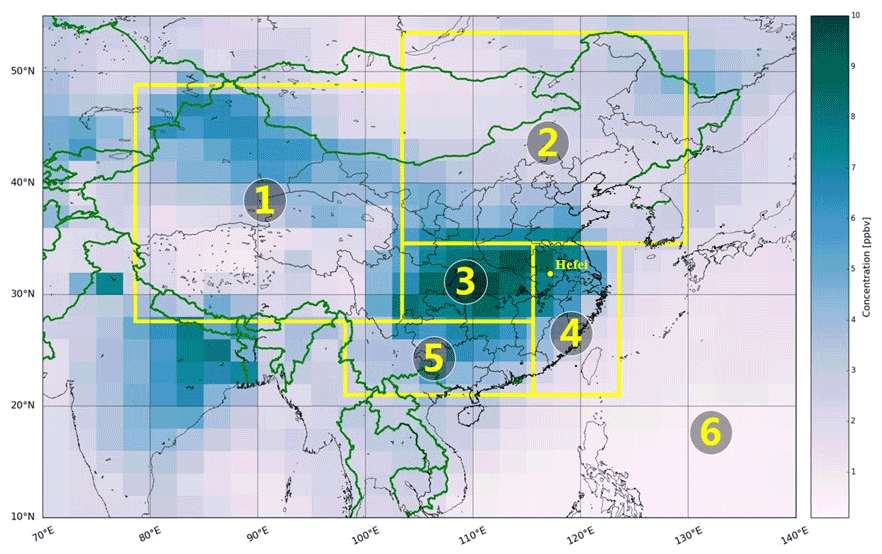
Figure 2 Geographical regions used for GEOS-Chem sensitivity simulations. The numbers ➀–➅ represent western, northern, central, eastern, and southern China, and the rest of world, respectively. See Table 3 for latitude and longitude delimitations. Daily mean values of C₂H₆ troDMF on 1 January 2017 provided by GEOS-Chem BASE simulation were selected as representative of wintertime enhancement in eastern China. The base map of this figure is created by the Python “Basemap” package.

Table 1 Error budget and degrees of freedom (DOFS) for signal of a randomly selected C₂H₆ troDMF retrieval over Hefei, eastern China.

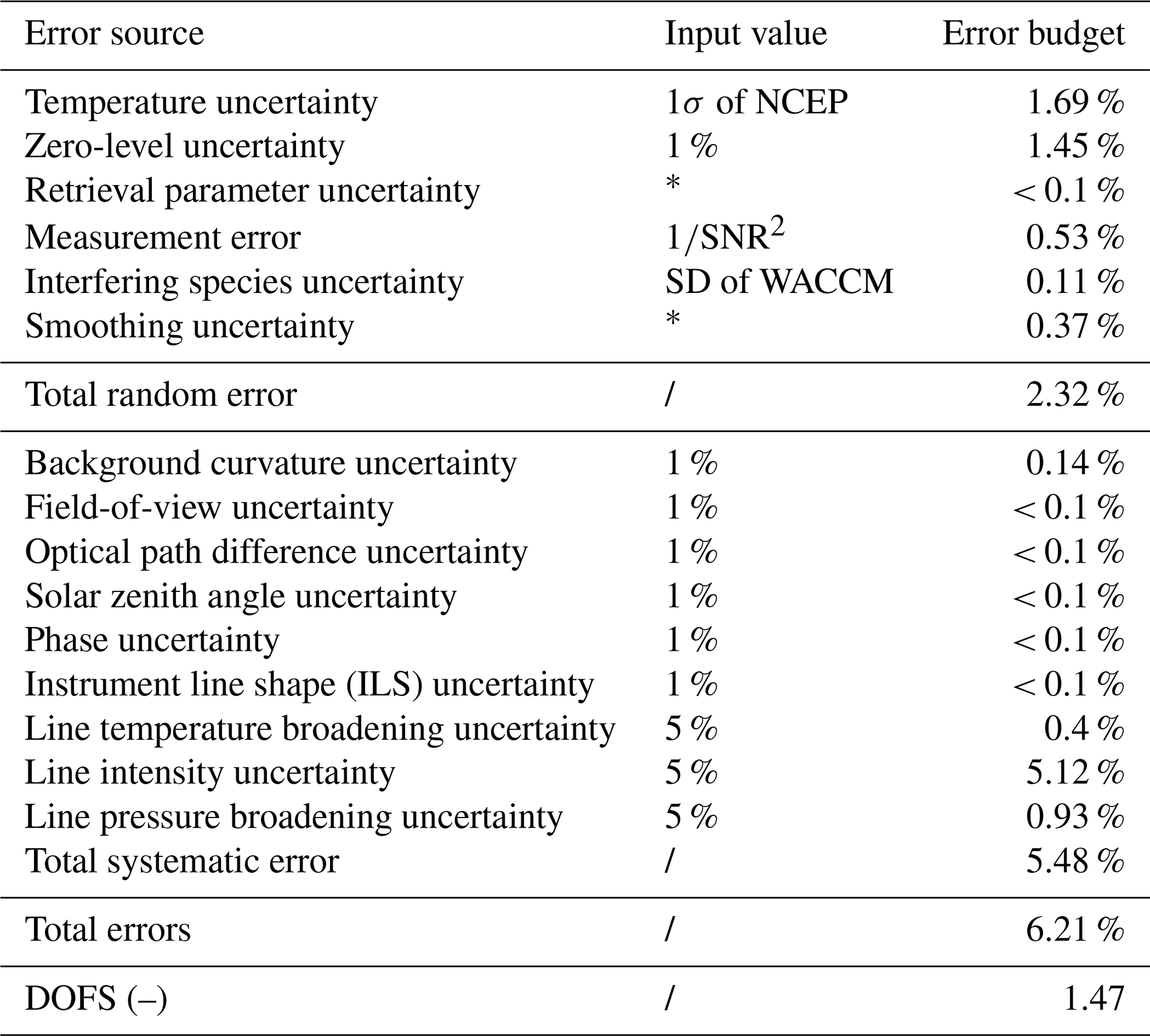
^* These input values for error budget estimation are based on the retrieval output.

We calculated the error budget for C₂H₆ retrieval at Hefei following the formalism of Rodgers (2000) and separated all error components into systematic or random errors according to whether they vary steadily or randomly over consecutive measurements. The random, systematic, and combined error budgets for the selected tropospheric layer (from the surface up to 10 km) are summarized in Table 1. The input covariance matrix of temperature is based on the differences between sonde and an ensemble of NCEP temperature profiles near Hefei, leading to 2–5 K in the troposphere and 3–7 K in the stratosphere. For each of the interfering gases, the corresponding covariance matrix is obtained with the WACCM v6 climatology. The input covariance matrix of the measurement error is based on the inverse square of the SNR of each spectrum. We regularly use a low-pressure HBr cell to diagnose the misalignment of the FTIR spectrometer and to realign the instrument when indicated. The FTIR spectrometer at Hefei is assumed to be not far from the ideal condition, and the input uncertainties for zero level, background curvature, field of view, optical path difference, solar zenith angle, interferogram phase, and ILS are estimated to be 1 %. For the C₂H₆ spectroscopic absorption coefficients, the line list in atm16 follows HITRAN2012 (Rothman et al., 2013), and we use 5 % for line intensity and pressure- and temperature-broadening coefficients. For the retrieval parameter and smoothing error, the input covariance matrices are prescribed from the optimal estimation retrieval outputs. To estimate the retrieval error of C₂H₆ troDMF at Hefei, the elements of all gain matrices were set to zero for the altitudes outside the selected layer. The contributions of all error components to C₂H₆ troDMF retrieval at Hefei are summarized in Table 1. The dominant random errors are from temperature uncertainty (1.69 %) and the zero-level uncertainty (1.45 %), and the dominant systematic error is from the line intensity uncertainty (5.12 %). Total random and systematic errors are estimated to be 2.32 % and 5.48 %, respectively. Total retrieval error, calculated as the square root sum of the squares of total random and systematic errors, is estimated to be 6.21 %.

In order to exclude measurements that were seriously affected by instable weather conditions or by the a priori profile due to low measurement information content under less favorable observational conditions (e.g., around noontime when the probed atmosphere is thinner or in summer when C₂H₆ is less abundant), the FTIR measurements saved with a solar intensity variation (SIV) of larger than 10 % or retrievals with total DOFS of less than 0.7 or a root mean square (RMS) of fitting residuals of larger than 2 %, which accounted for 11.2 % of total measurements, were excluded from this study.

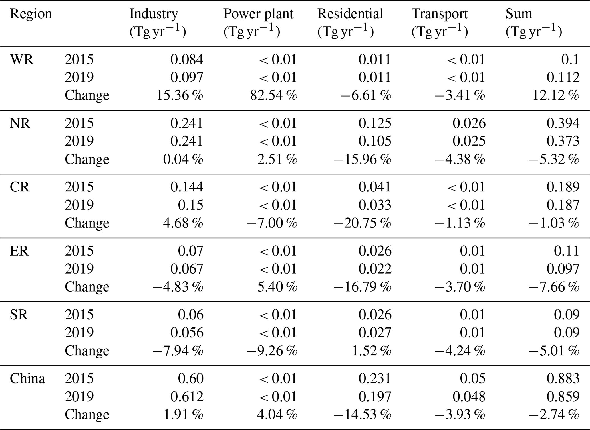
Table 2 Anthropogenic C₂H₆ emissions in China by region and category for the 2015 and 2019 Multi-resolution Emission Inventory for China (MEIC) emission inventories. WR refers to western China, NR refers to northern China, CR refers to central China, ER refers to eastern China, and SR refers to southern China.

2.2 GEOS-Chem sensitivity simulation

The relative contribution of various source categories and regions to the observed C₂H₆ variability were quantified by a series of sensitivity simulations using the GEOS-Chem chemical model version 12.2.1 (Bey et al., 2001) (http://geos-chem.org, last access on 24 August 2020). All simulations implemented a universal tropospheric–stratospheric chemistry (UCX) mechanism (Eastham et al., 2014; Fisher et al., 2017) and were driven by the Goddard Earth Observing System Forward Processing (GEOS-FP) meteorological fields at a degraded horizontal resolution of 2^∘ × 2.5^∘. The temporal resolutions are 1 h for surface meteorological variables and planetary boundary layer height (PBLH) and 3 h for other meteorological variables. The time steps used in the model are 10 min for transport and 20 min for chemistry and emissions, as recommend for the GEOS-Chem full-chemistry simulation at 2^∘ × 2.5^∘ (Philip et al., 2016). The nonlocal scheme for the boundary layer mixing process is described in Lin and McElroy (2010). Dry deposition was calculated by the resistance-in-series algorithm (Wesely, 1989; Zhang et al., 2001), and wet deposition followed that of Liu et al. (2001). The photolysis rates were available from the FAST-JX v7.0 photolysis scheme (Bian and Prather, 2002). All simulations were spun up for 1 year (July 2014 to July 2015) and output hourly mean C₂H₆ VMR profiles globally ranging from the surface to 0.01 hPa at a horizontal resolution of 2^∘ × 2.5^∘. This study only considered the C₂H₆ simulations from 2015 to 2020 in the grid box containing Hefei (31.52–32.11^∘ N by 116.53–118.02^∘ E).

In the recent past, the inventories led to significant underestimation of the C₂H₆ simulation (e.g., HTAP2 in Franco et al., 2016). Since then, some efforts have improved the situation (e.g., Tzompa-Sosa et al., 2017). In this study, we refer to Sun et al. (2020a) for more details on the implementation of emission inventories. Briefly, global anthropogenic emissions were from the Community Emissions Data System (CEDS) inventory which is overwritten in Asia by the latest Multi-resolution Emission Inventory for China (MEIC) (Hoesly et al., 2018; Li et al., 2017; Lu et al., 2019; Zheng et al., 2018). Global biomass burning and biogenic emissions were from the Global Fire Emissions Database (GFED v4) inventory (Giglio et al., 2013) and the Model of Emissions of Gases and Aerosols from Nature (MEGAN version 2.1) inventory (Guenther et al., 2012), respectively. The CH₄ emission fields are prescribed based on NOAA measurements for 1983–2016 and are extended to 2020 using the linear extrapolation of local 2011–2016 change rates (Murray, 2016; Lu et al., 2019).

Table 3 GEOS-Chem model configurations and delimitations of all geographical regions used in sensitivity simulations. FF refers to fossil fuel, BVOCs refer to biogenic volatile organic compounds, BB denotes biomass burning, and BIOF refers to biofuel.

Particular improvements have been made for the latest bottom-up MEIC emission inventory with respect to the accuracy of vehicle emission modeling (Zheng et al., 2014), power plant emission calculation (Liu et al., 2015), and the non-methane VOC (NMVOC) speciation method (Li et al., 2014). Many studies have verified that the MEIC emission inventory can reasonably represent the anthropogenic emissions over Asia (Hoesly et al., 2018; Li et al., 2017; Lu et al., 2019; Y. Sun et al., 2021; Tian et al., 2018; Yin et al., 2020, 2019; Zheng et al., 2018). Anthropogenic C₂H₆ emissions in China by region and category for the 2015 and 2019 MEIC emission inventories are summarized in Table 2. All subdivided geographical regions are shown in Fig. 2, and the resulting delimitations are summarized in Table 3. The delimitations of these geographical regions are based on the levels of urbanization and industrialization in China. Region ➀ in Fig. 2 only covers a few sparse city clusters, representing the region with lowest population and least industrialization in China (Lu et al., 2019). Regions ➁, ➃, and ➄ cover the North China Plain (NCP), the Yangtze River Delta (YRD), and the Pearl River Delta (PRD) city clusters, respectively, which are the three most developed city clusters facing severe air pollution in China. Region ➂ covers the Sichuan Basin (SCB) and central Yangtze River (CYR) city clusters, representing newly emerging severe air pollution in China. Total annual Chinese anthropogenic emissions of C₂H₆ in 2015 and 2019 are 0.883 and 0.859 Tg, respectively. In both years, anthropogenic C₂H₆ emissions in China are dominated by industrial and residential emissions. The highest anthropogenic C₂H₆ emission rates (calculated as the ratio of total C₂H₆ emission to the coverage) are in the densely populated and industrialized clusters in the eastern part of China (including northern China (NR), eastern China (ER), central China (CR), southern China (SR), and the adjacent regions) with large seasonal variation (Fig. S1 in the Supplement). The highest anthropogenic C₂H₆ emissions typically occur in winter (Fig. S1). The anthropogenic emissions in the WR region are typically lower than those in other parts of China because of a lower population and less industry in the region (Lu et al., 2019; Zheng et al., 2018).

In order to quantify the contributions of different source categories and regions to the observed C₂H₆, we first conducted a reference full-chemistry simulation (BASE) with the implementation of all emission inventories as described above. We then conducted a series of sensitivity simulations to assess the change in each sensitivity simulation relative to the BASE simulation. Model configurations in this study were similar to those in Y. Sun et al. (2021) but with a different emission perturbation method. When an emission inventory was shut off in Y. Sun et al. (2021), the emissions of all atmospheric compounds in that inventory were suppressed. In contrast, this work only suppressed C₂H₆ in each case except for biogenic and biomass burning emission perturbations, which suppressed all atmospheric compounds as we cannot separate C₂H₆ emission from current biogenic and biomass burning emission inventories. Model configurations in this study are summarized in Table 3 and were described as follows:

• i.

  To analyze the contributions of different emission categories, we shut off C₂H₆ in each individual emission inventory to evaluate the change in the simulation in the presence of C₂H₆ in other emission inventories. As a result, the relative contribution of each emission category was estimated as the relative difference between the GEOS-Chem simulation in the presence and absence of C₂H₆ in that emission inventory. We have conducted four such sensitivity simulations by shutting off C₂H₆ emissions in (1) the fossil fuel emission inventory (including emissions from agriculture, industry, power plant, residential, and transport), (2) the biogenic emission inventory, (3) the biomass burning emission inventory, and (4) the biofuel emission inventory (Table 3). The sum of fossil fuel and biofuel C₂H₆ emissions is defined as an anthropogenic C₂H₆ source, and the sum of biogenic and biomass burning C₂H₆ emissions are referred to as a natural C₂H₆ source.

• ii.

  To analyze the contributions of different geographical regions, we shut off all categories of C₂H₆ emissions (i.e., the aforementioned anthropogenic and natural C₂H₆ sources) within each geographical region to assess the change in the simulation in the presence of C₂H₆ emissions outside that geographical region. Thus, the relative contribution of each geographical region was estimated as the relative difference between the GEOS-Chem simulation in the presence and absence of C₂H₆ emissions within that geographical region. We have conducted five such sensitivity simulations by shutting off C₂H₆ emissions within five geographical regions, as shown in Fig. 2.

2.3 Generalized additive models (GAMs) regression

In this study, we investigate the dependencies of C₂H₆ on meteorological and emission factors using GAMs regression (Wood and Simon, 2004; Wood, 2004). Regression analysis is proceeded using the thin plate smoothing spline function (Pearce et al., 2011). Smoothing parameters and confidence intervals are calculated according to the restricted maximum likelihood standard (REML) and the unconditional Bayesian method, respectively (Pearce et al., 2011). GAMs regression is better than the traditional statistical models in dealing with nonlinear fittings (Veaux and Richard, 2012). For climate change applications, where there are many nonlinear relationships between variables, GAMs regression is particularly attractive (Zhang et al., 2019).

We introduced a variety of potential meteorological and emission factors into the GAMs regression one at a time and performed significance tests based on the Akaike information criteria (AIC) values (Wood and Simon, 2004). The explanatory variables which passed the significance tests with the smallest AIC values were included into the final GAMs model. Furthermore, explanatory variables in GAMs regression may interact with each other and result in unstable fittings due to the internal multicollinearity. For the explanatory variables that show a strong collinearity with each other, we only included one of them in the final GAMs model. The degree of multicollinearity can be quantified by the variance inflation factor (VIF) (Ma et al., 2020). Generally, a stronger collinearity between the explanatory variables results in a larger VIF, and the VIF of an explanatory variable could be 1.0 if it is not correlated with other explanatory variables (Ma et al., 2020). In this study, we included all of the meteorological and emission factors in the GAMs and calculated the VIF for all of the influencing factors. The multicollinearity diagnosis concluded that the main causes of multicollinearity are between the HCN and CO and between the tropopause height and the PBLH. Including either of these two data pairs in the GAMs regression showed significant collinearity with VIF values of greater than an empirical threshold of 4.0, indicating an unstable regression (Lin et al., 2018). After omitting HCN and PBLH in the final GAMs model, the adjusted VIF values of all the variables were less than 4.0 and the variables uniformly passed the significance tests. As a result, the final GAMs model in the context of the C₂H₆ troDMF time series y can be described as follows (Pearce et al., 2011):

$$\begin{array}{}\text{(1)}& \begin{array}{rl}\log \left(y\right)=& \mathit{\beta }+S\left(\text{ua}\right)+S\left(\text{va}\right)+S\left(\text{omega}\right)+S\left(\text{qv}\right)\\ & +S\left(\text{troph}\right)+S\left(\text{pres}\right)+S\left(\text{temp}\right)+S\left({\mathrm{CH}}_{\mathrm{4}}\right)\\ & +S\left(\text{CO}\right)+\mathit{\epsilon },\end{array}\end{array}$$

where β and ε are the mean response constant and the fitting residual, respectively. S(ua), S(va), S(omega), S(qv), S(troph), S(pres), S(temp), S(CH₄), and S(CO) are the smoothing functions of daily average zonal wind (m s⁻¹), meridional wind (m s⁻¹), vertical wind (Pa s⁻¹), water vapor concentration (%), tropopause height (km), pressure (hPa), temperature (^∘C), CH₄ troDMF (ppbv), and CO troDMF (ppbv). Positive values of ua, va, and omega represent northward, eastward, and upward winds, respectively. The sum of S(CH₄) and S(CO) is referred to as the emission influences, and the sum of the remaining smoothing functions is referred to as the meteorological influences.

To drive the GAMs regression, we first derived CH₄ and CO VMR profiles from direct solar absorption spectra similar to that of C₂H₆ (see Sect. 2.1). The spectra for CH₄ retrievals are exactly the same as those of C₂H₆, but the spectra for CO are saved at a different filter channel. The respective VMR profiles were then converted to troDMF values following the method of C₂H₆. The retrieval configurations, wave band selections and the interfering gases considerations for CH₄ and CO can be found in Sun et al. (2018b). The DOFS of the retrievals between the surface and 10 km altitude for both CH₄ and CO are larger than 1.5, and the corresponding retrieval errors are less than 8 % (Sun et al., 2018b). All meteorological factors are from the GEOS-FP meteorological fields at their native resolution of 0.25^∘ × 0.3125^∘ ranging from the surface to 0.01 hPa at a temporal resolution of 1 h. As the meteorological fields and C₂H₆ concentration are not uniformly distributed along the altitude, the summing mean values of the meteorological fields cannot properly characterize the meteorological influences. In this study, we use a method similar to that of Shaiganfar et al. (2017) to increase the influence weighting toward the lower troposphere. As a result, all meteorological parameters except tropopause height (troph) are converted into the C₂H₆ profile weighting averaged value ω_avg through Eq. (2):

$$\begin{array}{}\text{(2)}& {\mathit{\omega }}_{\text{avg}}={\displaystyle \frac{{\sum }_i\mathit{\omega }\left(z_i\right)\cdot c\left(z_i\right)\cdot \text{Air mass}\left(z_i\right)}{{\sum }_{i}c\left(z_i\right)\cdot \text{Air mass}\left(z_i\right)}},\end{array}$$

where ω(z_i), c(z_i), and Air mass(z_i) represent the value of the meteorological factor, C₂H₆ concentration, and the air mass at the altitude z_i, respectively.

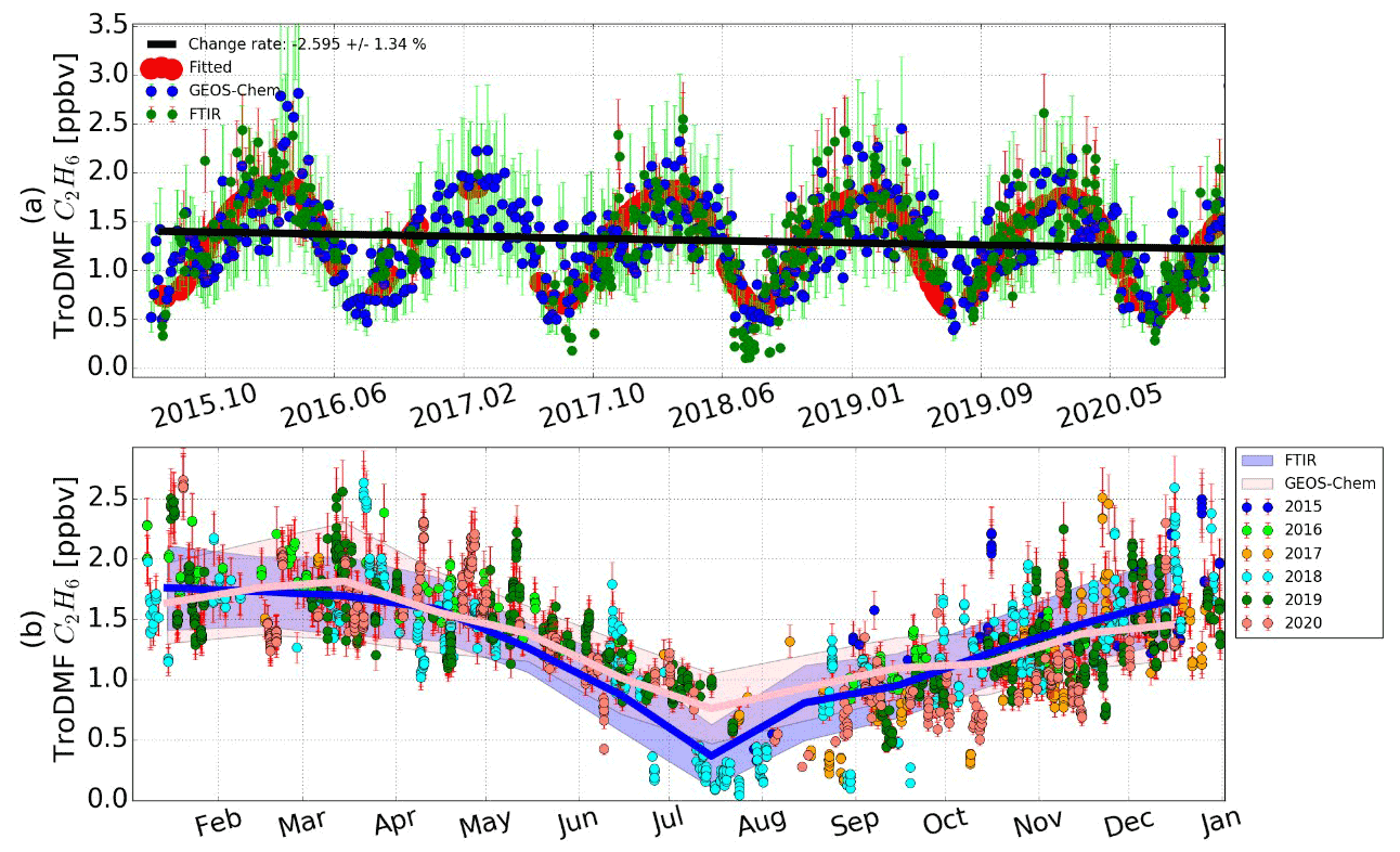
Figure 3 (a) C₂H₆ troDMF time series comparison between the FTIR observation and GEOS-Chem model BASE simulation from 2015 to 2020 over Hefei, eastern China. The seasonality and interannual variability are represented by red dots and a black line, respectively, which are fitted using a bootstrap resampling model with a third Fourier series and a linear function. (b) Seasonal variations in C₂H₆ troDMF by FTIR and GEOS-Chem simulation. The bold curves and the shadows are the monthly mean values and the 1σ standard variations, respectively. Vertical error bars for FTIR and GEOS-Chem represent retrieval uncertainties and diurnal variabilities, respectively. A retrieval error of 6.21 % in Table 1 was used to estimate the absolute uncertainties of all observations. As a result, the absolute uncertainties in winter are larger than those in summer due to a higher C₂H₆ level in the season.

3 Variability and comparison with GEOS-Chem model data

We have compared the observed daily mean time series, seasonal cycle, and interannual variability of C₂H₆ troDMF to the GEOS-Chem BASE simulations for investigating the chemical model performance for specific polluted regions over eastern China. As the vertical resolution of GEOS-Chem is different from the FTIR observation, smoothing correction has been carried out for the GEOS-Chem profiles (Rodgers and Connor, 2003). First, the GEOS-Chem daily mean profiles of C₂H₆ have been interpolated to the FTIR altitude grid to ensure a common altitude grid. In order to match observations from the FTIR which only operates during daytime, the average for GEOS-Chem simulations was only performed during daytime from 09:00 to 17:00 LT (local time). The interpolated profiles were then smoothed by the concurrent seasonal mean values of the FTIR averaging kernels and a priori profiles (Rodgers, 2000; Rodgers and Connor, 2003). The smoothed GEOS-Chem profiles were subsequently converted to troDMF values using the corresponding regridded air density profiles from the model with the method described in Sect. 2.1. Finally, the GEOS-Chem C₂H₆ troDMF time series only for the days with available FTIR observations were averaged by month and compared with the FTIR monthly mean data.

Figure 3a shows the comparison of daily mean time series of C₂H₆ troDMF between the FTIR observation and the smoothed GEOS-Chem model simulation from 2015 to 2020. Figure 3b compares the seasonal cycles derived from Fig. 3a for the days with available FTIR observations only. Generally, the measured features in terms of seasonality and interannual variability can be reproduced by the GEOS-Chem simulations with a correlation coefficient (r) of 0.88 (Fig. S2). Large GEOS-Chem vs. FTIR differences tended to occur in the trough and peak of the observations. For instance, the observed monthly mean value of C₂H₆ troDMF was overestimated by 35.6 % (calculated as (GEOS-Chem − FTIR) $/$ FTIR) in July and underestimated by 14.6 % in December by GEOS-Chem. These discrepancies may be mainly attributed to uncertainties in the horizontal transport and vertical mixing schemes simulated by the GEOS-Chem model at a relatively coarse spatial resolution, which are difficult to match column observation over a single point. In addition, the number of C₂H₆ measurements at Hefei on each measurement day varied a wide range from 1 to 17 depending on the weather conditions, but GEOS-Chem simulations are available consecutively by hour for the same day. This difference in the temporal resolution of GEOS-Chem and FTIR could also cause inconsistencies due to the high variability of atmospheric C₂H₆. However, considering the concurrent data pairs only (± 30 min), the averaged difference between GEOS-Chem and FTIR data (GEOS-Chem − FTIR) is (−0.02 ± 0.05) ppbv (−1.6 ± 4.2) %, which is within the FTIR uncertainty budget. As a result, GEOS-Chem can simulate the C₂H₆ concentration and variability for specific polluted regions over eastern China. With improved emission inventories, previous studies have also found that global chemistry transport models were able to reproduce the absolute values as well as seasonal cycles of the ground-based FTIR C₂H₆ observations in other parts of the world (Franco et al., 2015, 2016; Tzompa-Sosa et al., 2017).

As typically observed, the peak-to-peak amplitude of the modulation with respect to the monthly mean of C₂H₆ troDMF spanned a large range from −16.0 % to 72.8 % depending on season (Fig. 3b). The observed C₂H₆ troDMF roughly decreases over time for the first half of the year and increases over time for the second half of the year (Fig. 3b). High levels of C₂H₆ troDMF occur in the late autumn to early spring, and low levels of C₂H₆ troDMF occur in late spring to early autumn. The observed C₂H₆ troDMF reached a minimum monthly mean value of (0.36 ± 0.26) ppbv in July and a maximum monthly mean value of (1.76 ± 0.35) ppbv in December. C₂H₆ troDMFs in December were on average 4.9 times higher than those in July. As the tropospheric OH oxidation capability in summer is higher than that in winter, the C₂H₆ seasonality characterized by a winter maximum and a summer minimum was also observed in other FTIR stations (Angelbratt et al., 2011; Franco et al., 2015, 2016; Lutsch et al., 2019; Nagahama and Suzuki, 2007; Rinsland et al., 2002; Simpson et al., 2012; Viatte et al., 2015, 2014; Vigouroux et al., 2012; Zeng et al., 2012; Zhao et al., 2002). We have used the bootstrap resampling method of Gardiner et al. (2008) to evaluate the seasonality and interannual variability of C₂H₆ troDMF, where a third Fourier series and a linear function were used to fit daily mean time series of C₂H₆ troDMF from both FTIR observations and GEOS-Chem model simulations. We incorporated the errors arising from the autocorrelation in the residuals into the uncertainties in the change rates following the procedure of Santer et al. (2008). The observed C₂H₆ troDMFs from 2015 to 2020 showed a negative change rate of (−2.60 ± 1.34) % yr⁻¹, which is in reasonable agreement with the modeled change rate of (−2.1 ± 0.7) % yr⁻¹ (Fig. 3a).

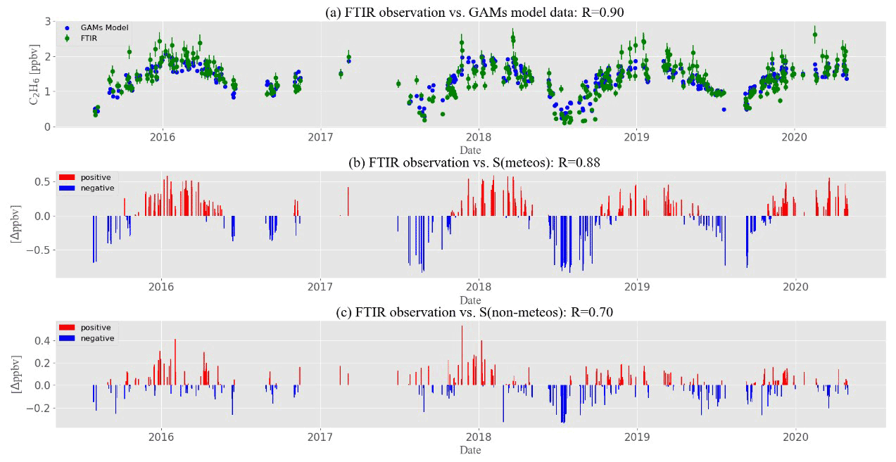
Figure 4 (a) C₂H₆ troDMF time series from 2015 to 2020 over Hefei, eastern China, from FTIR and the GAMs regression model. (b) Time series of accumulated meteorological smooth functions, S(meteos); (c) time series of accumulated emission smooth functions, S(non-meteos). Positive and negative influences are indicated using red and blue bars, respectively. Correlation coefficients for the total, meteorological, and emission influences are also shown.

4 GAMs regression results and interpretation

C₂H₆ troDMF time series from 2015 to 2020 over Hefei from the FTIR and the GAMs regression model are shown in Fig. 4. The observed C₂H₆ variability can be reproduced by the GAMs regression model with good agreement, as confirmed by a correlation coefficient (r) of 0.90 (Figs. 4a, S3). Meanwhile, the observed C₂H₆ troDMF time series also show high correlations with both the accumulated meteorological factor (r = 0.88) (Fig. 4b) and the accumulated emission factor (r =  0.70) (Fig. 4c), indicating that both meteorological and emission influences are important factors for driving the C₂H₆ troDMF variability. Generally, both meteorological and emission factors show positive influences on C₂H₆ troDMFs in the cold season (December–January–February/March–April–May, DJF/MAM) and negative influences on C₂H₆ troDMFs in the warm season (June–July–August/September–October–November, JJA/SON). However, the seasonal dependency of meteorological influence is stronger than that of emission influence. During the studied years, the year-to-year differences in meteorological influence are small, and the positive emission influence showed an overall decreasing change rate from 2016 onward, which has probably driven a decreasing change rate in C₂H₆ troDMF in recent years.

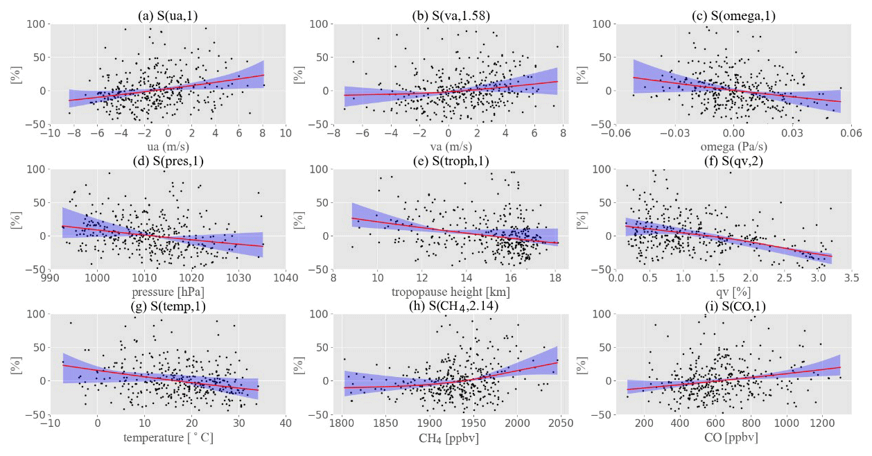
Figure 5 The influence of each individual variable in the GAMs model on C₂H₆ troDMF from 2015 to 2020 over Hefei, eastern China. Panels (a)–(i) are for zonal wind (ua), meridional wind (va), convection wind (omega), pressure (pres), tropopause height (troph), H₂O troDMF (qv), temperature (temp), CH₄ troDMF (CH₄), and CO troDMF (co), respectively. The DOFS of each smoothing function is included in the parenthetical information in each panel heading. The x axis represents the variation range of each variable, and the y axis represents the relative percentage change in C₂H₆ troDMF relative to its annual mean value.

The influence of each explanatory variable x_i in GAMs regression, calculated as $\mathrm{100}\mathit{\%}\cdot [{\mathrm{e}}^{s\left(x_i\right)}-\mathrm{1}]$, is shown in Fig. 5, which reflects the influence of each individual variable on the relative change in C₂H₆ troDMF. The corresponding DOFS of each smoothing function are also shown in Fig. 5. If an explanatory variable is linearly correlated with C₂H₆ troDMF, the DOFS of the resulting smoothed variable could be equal to 1, and the larger the slope, the higher the linear response. Otherwise, the larger the deviation of DOFS relative to 1, the more significant the nonlinear relationship (Veaux and Richard, 2012). During the studied years, the DOFS of zonal wind (ua), convection wind (omega), pressure (pres), tropopause height (troph), temperature (temp), and CO troDMF (co) were close to 1, reflecting a roughly linear relationship of these explanatory variables with C₂H₆ troDMF. In contrast, the DOFS of meridional wind (va), H₂O troDMF (qv), and CH₄ troDMF (CH₄) were much greater than 1, reflecting a significant nonlinear relationship with C₂H₆ troDMF.

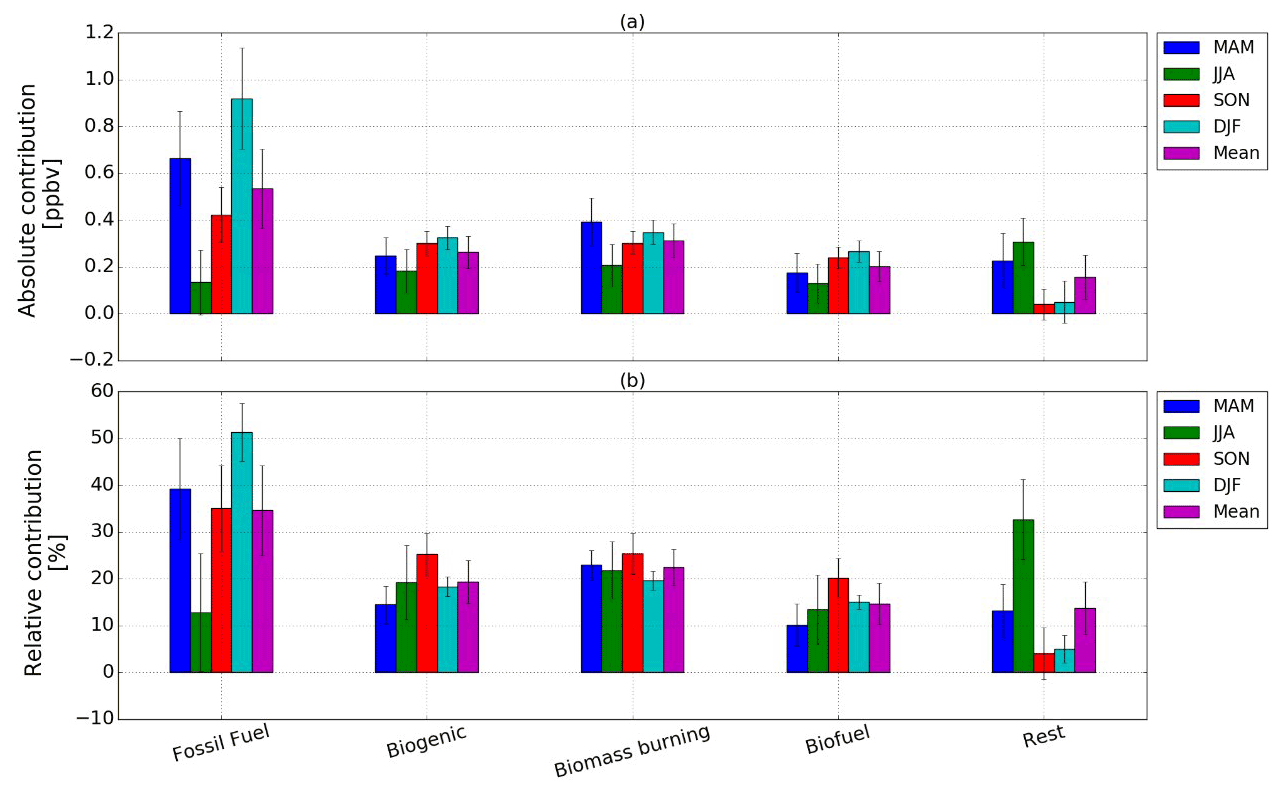
Figure 6 Absolute (a) and relative (b) contributions of fossil fuel, biogenic, biomass burning, and biofuel emission sources to the observed C₂H₆ variability from 2015 to 2020 over Hefei, eastern China. The remaining contribution, calculated as the difference between the BASE simulation and the sum of anthropogenic and natural contributions, is also shown. All contributions are grouped by season. Vertical error bars represent 1σ standard variation.

The observed C₂H₆ troDMF was influenced by many factors. The zonal wind (ua), meridional wind (va), CH₄ troDMF (CH₄), and CO troDMF (co) showed positive influences on the observed C₂H₆ troDMF variability, whereas the other explanatory variables showed negative influences. The results show that the northward, eastward, and downward convection winds facilitate the accumulation of C₂H₆ over the observation site and result in higher C₂H₆ troDMF. As most anthropogenic and biomass burning sources of CO as well as fossil fuel sources of CH₄ are common sources of C₂H₆, C₂H₆ troDMF gradually went up as CH₄ and CO troDMFs increased. In contrast, meteorological conditions such as high temperature, high humidity, and low pressure are more favorable to C₂H₆ oxidation, resulting in lower C₂H₆ troDMF. Meanwhile, deep upward convective winds and high tropopause height facilitate the removal of C₂H₆ over the observation site and result in lower C₂H₆ troDMF.

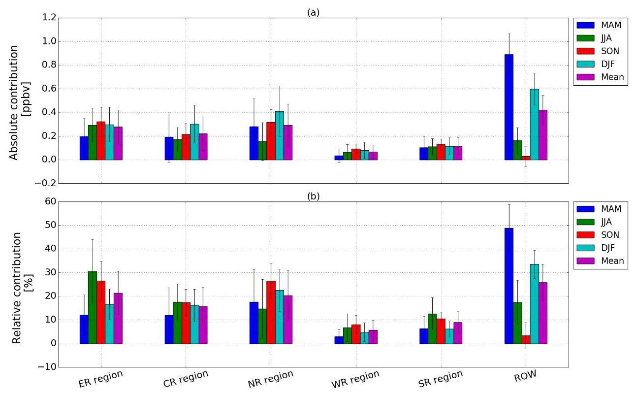
Figure 7 Absolute (a) and relative (b) contributions of ER, CR, NR, WR, SR, and ROW regions to the observed C₂H₆ variability from 2015 to 2020 over Hefei, eastern China. All contributions are grouped by season. The geographical definition of each region is summarized in Table 3. Vertical error bars represent 1σ standard variation.

5 Source attribution

5.1 Contributions of different source categories and regions

The absolute and relative seasonal contributions of fossil fuel, biogenic, biomass burning, and biofuel emissions to C₂H₆ variability from 2015 to 2020 over Hefei are shown in Fig. 6. The GEOS-Chem annual mean C₂H₆ troDMF simulations were decreased by 0.51, 0.27, 0.32, and 0.20 ppbv in the absence of fossil fuel, biogenic, biomass burning, and biofuel C₂H₆ emission inventories, which correspond to 34.6 %, 18.4 %, 21.3 %, and 13.5 % of the relative contribution to the modeled C₂H₆ variability, respectively. The anthropogenic emissions account for 48.1 % of the C₂H₆ variability, and the natural emissions account for 39.7 %. The remaining, contribution calculated as the difference between the BASE simulation and the sum of anthropogenic and natural contributions, is 0.17 ppbv (12.2 %). This missing contribution can be largely attributed to nonlinear interactional effects among different sources which were not captured by the sensitivity simulations. Indeed, shutting off an emission inventory may induce significantly lower concentrations in atmospheric compounds (i.e., C₂H₆ for noFF and noBIOF or all suppressed compounds for noBVOC and noBB simulations; see Table 3 for an explanation of these terms) globally. On the one hand, some of them may react with OH, which would lead to higher OH concentrations being available for the oxidation of C₂H₆, eventually enhancing the C₂H₆ destruction from other emission categories. On the other hand, some of them may form OH by a series of oxidation reaction, which would lead to lower OH concentrations being available for the oxidation of C₂H₆, eventually mitigating the C₂H₆ destruction from other emission categories. However, it is difficult to quantify the nonlinear impact of each individual emission category, as the concentration and spatial distribution of C₂H₆ in each emission category are different. Especially when biogenic and biomass burning emissions are suppressed, the impacts become hard to assess, as all NMVOC compounds play a key role in both OH formation and destruction. Investigating the nonlinear impact of each individual emission category would require additional work that is beyond the scope of the present study.

The contributions of all emission sources are dependent on season, and the fossil fuel contribution shows the largest seasonal difference, which consolidates the GAMs regression results that the emission influences are seasonally dependent. The fossil fuel contributions in winter and spring (DJF/MAM) are larger than those in summer and autumn (JJA/SON), with a maximum of 52.0 % in DJF and a minimum of 13.0 % in JJA. The JJA/SON meteorological conditions which show stronger solar radiation, higher temperature, wetter atmospheric condition, and lower pressure than those in DJF/MAM are more favorable for increasing VOC emissions from biogenic sources (BVOCs), which consolidates the fact that C₂H₆ abundance from biogenic source in JJA/SON is larger than that in DJF/MAM. The missing remainder contributes to a maximum of 32 % in JJA when the C₂H₆ oxidation reaches the seasonal maximum and is, thus, more sensitive to the on–off state of different sources.

Figure 7 explores the absolute and relative seasonal contributions of the ER, CR, NR, WR, and SR regions to the C₂H₆ variability from 2015 to 2020 over Hefei. The GEOS-Chem annual mean C₂H₆ troDMF simulations were decreased by 0.28, 0.22, 0.29, 0.07, and 0.12 in the absence of C₂H₆ emissions in the ER, CR, NR, WR, and SR regions, which correspond to 21.5 %, 15.8 %, 20.3 %, 5.7 %, and 8.9 %, of the relative contribution to the modeled C₂H₆ variability, respectively. The contributions of all geographical regions are also seasonally dependent. The results show that the observed C₂H₆ variability was largely attributed to emissions within China (74.1 %), which show a maximum in JJA/SON and a minimum in DJF/MAM. Due to their vicinity to the observation site, the ER, CR, and NR regions dominated the contribution within China (57.6 %). The remaining contribution, calculated as the difference between the BASE simulation and the total contributions of above individual source regions, is 0.42 ppbv (25.9 %). This contribution is the sum of the C₂H₆ emissions outside China (ROW – rest of the world) and the nonlinear interactional effects among the geographical sensitivity simulations. This remaining contribution in DJF/MAM is ∼ 4.0 times larger than that in JJA/SON. Considering that the nonlinear interactional effects mainly occur in JJA/SON, but this remaining contribution shows a seasonal minimum value in the meantime, the remaining contribution can be largely attributed to ROW contributions.

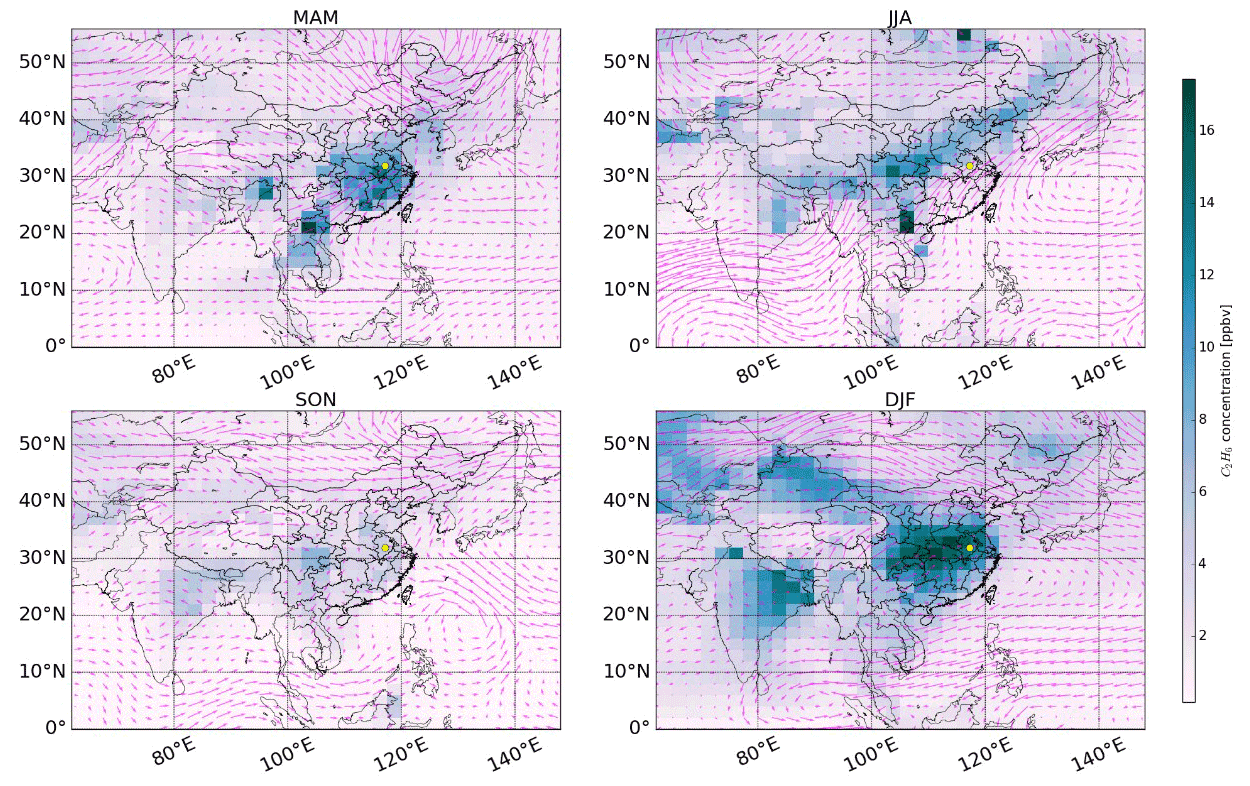
Figure 8 Spatial distribution of C₂H₆ troDMF in the GEOS-Chem BASE simulations in different seasons. The arrows indicate horizontal wind vectors at 900 hPa; the observation site is marked with a yellow dot. Meteorological fields are from the GEOS-FP 0.25^∘ × 0.3125^∘ dataset.

As a relatively long-lifetime species (a few months), C₂H₆ emissions originating from either nearby or in distant areas can be transported to the Hefei site under favorable weather conditions and, thus, contribute to the observed C₂H₆ variability. In addition, atmospheric compounds originating either nearby or in distant areas, which affect the chemistry of C₂H₆ oxidation, could also affect the observed C₂H₆ variability. For contributions within China, the lowest contribution of the WR region to the observed C₂H₆ variability is largely attributed to the lowest C₂H₆ emission rates in this region (Table 2). The smaller contribution of the SR region to the observed C₂H₆ variability in DJF/MAM in comparison with the ER, CR, and NR regions is mainly attributed to fewer air masses that originated in south China under the dry winter monsoon conditions (see Sect. 5.2).

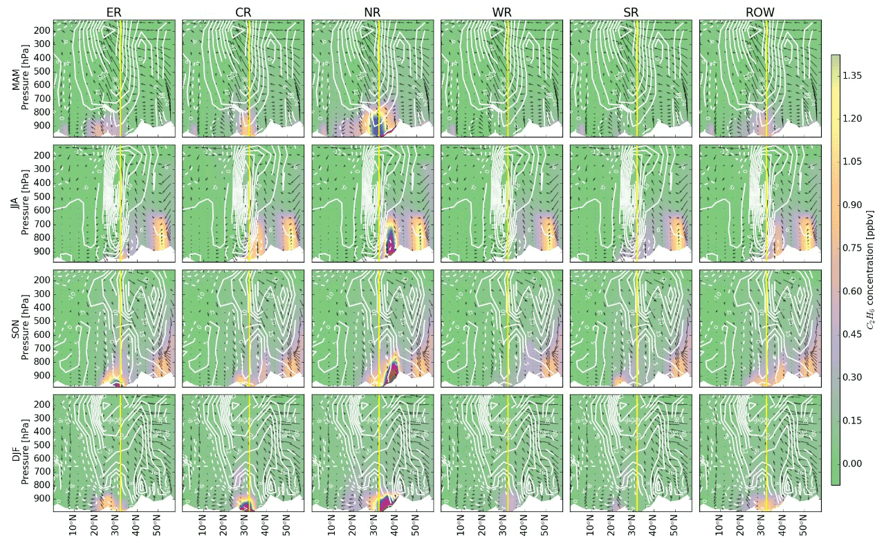
Figure 9 The first row shows the latitude–height distributions of the C₂H₆ VMR averaged over 113–121^∘ E in spring (MAM), originating from different source regions (corresponding to different columns). See Table 3 for latitude and longitude definitions. The white area indicates topography, and the white contours at intervals of 6 m s⁻¹ are the easterly (dashed) and westerly (solid) mean meridional winds; the wind vectors (consisting of zonal wind in m s⁻¹ and vertical velocity in units of Pa s⁻¹) are represented by arrows; the observation site is marked with a yellow line. The second to fourth rows are the same as the first row but for summer (JJA), autumn (SON), and winter (DJF), respectively. Meteorological fields are from the GEOS-FP 0.25^∘ × 0.3125^∘ dataset.

5.2 Transport inflow and outflow pathways

The direct GEOS-Chem sensitivity simulations can clearly characterize the 3D transport inflow and outflow pathways of C₂H₆ over the observation site. Figure 8 shows the spatial distribution of the GEOS-Chem C₂H₆ BASE simulations around China along with horizontal wind vectors at 900 hPa in different seasons. General atmospheric circulation patterns over eastern China are typically affected by midlatitude westerlies and the Asian monsoon, including the East Asian summer monsoon and the South Asian summer monsoon (Chen et al., 2009; Liang et al., 2005; Liu et al., 2003). Figure 9 illustrates the latitude–height distributions of the C₂H₆ VMR over China from six source regions along with the 3D atmospheric circulation patterns in different seasons. Thus, the 3D transport inflow and outflow pathways of C₂H₆ over the observation site are deduced as follows.

As indicated by the arrows in Figs. 8 and 9, the high-pressure system over the Eurasian continent in DJF triggers the descent of very cold air over eastern China and results in air masses converging toward the observation site from the western and northern areas, while the high-pressure system over the Indian Ocean and the Pacific in JJA triggers the ascent of strongly heated air over eastern China and results in air masses converging toward the observation site from South Asia and East Asia (SEAS) (Liang et al., 2004; Liu et al., 2003). In DJF, the midlatitude westerlies extend to the tropics (about 15^∘ N) over the middle and upper troposphere and to the subtropics (about 30^∘ N) near the surface, while the easterlies mainly prevail in the tropics and are weak over eastern China (Figs. 8, 9). In the summer monsoon season, the atmospheric circulation patterns over eastern China change dramatically and are dominated by a surface wind regime originating from the Pacific, the South China Sea, or the Arabian Sea (Figs. 8, 9). Meanwhile, the midlatitude westerlies recede to the north temperate zone (north of 30^∘ N) and the westerly jet center shifts to north of 50^∘ N in JJA (from ∼ 30^∘ N in DJF) (Fig. 8). In JJA, the tropical region is characterized by strong easterlies in the upper troposphere and by southwesterly air flow in the lower troposphere (Fig. 9). The prevailing winds in the transition seasons in MAM and SON are still westerlies with frequent cold fronts (Figs. 8, 9). These abovementioned seasonal circulation patterns determine the transport inflow and outflow of C₂H₆ around the observation site. However, the transport scales are also influenced by source location and strength, travel trajectory, and travel time (Liu et al., 2003).

Generally, C₂H₆ emissions from the CR, NR, and WR regions can be transported to the observation site by strong westerlies throughout the year (Fig. 9). C₂H₆ from the SR region can be transported to the observation site by deep convection followed by northward transport into the midlatitude westerlies in MAM or driven by the South Asian summer monsoon or westerlies in other seasons (Liu et al., 2003) (Fig. 8). The observed C₂H₆ transport inflow originating from the local ER region is mainly driven by the local circulation cell or Asian monsoon. The driver for C₂H₆ transport inflow originating from the northern ROW (> 32^∘ N) is the same as those from the CR, NR, and WR regions. The driver for C₂H₆ transport inflow originating from the southern ROW (< 32^∘ N) is the same as that from the SR region. However, C₂H₆ originating from ROW relative to those from China reaches a higher altitude due to longer transport distances. The fact that the ROW contributions in JJA/SON are lower than those in DJF/MAM can be partly attributed to stronger removal along the long-range transport pathway by abundant wet precipitation and oxidation during the summer monsoon and post-monsoon season.

Seasonal variability in C₂H₆ transport outflow over the observation site is mainly associated with the monsoon system. In DJF, C₂H₆ over the observation site is capped in the lower troposphere by the subsidence over eastern China and is swept southwestward by northeasterly winds into southwestern areas, where it is lifted up into the free troposphere by convection and then flows away northeastward (Fig. 9). In JJA, the observed C₂H₆ is transported northeastward by the Asian monsoon and undergoes frequent lifting into the upper troposphere by deep convection (Figs. 8, 9). Frequent cold fronts are common phenomena during meteorological transitional periods in MAM and SON. In SON, the winter monsoon builds a continental high system, and sweeps the observed C₂H₆ in the lower troposphere northward to relatively high latitudes where it can be lifted up into the free troposphere by deep convection or cold fronts. In MAM, convection at lower latitudes over the Asian continent starts to rise, which lifts the observed C₂H₆ up into the free troposphere before it then flows away southward.

5.3 Potential factors driving interannual variability of C₂H₆

China has implemented a series of active clean air policies since 2013 to mitigate severe air pollution problems (Sun et al., 2020; Zhang et al., 2019; Zheng et al., 2018). Since then, the emissions of major air pollutants have decreased, and the overall air quality has greatly improved (Sun et al., 2020; Zhang et al., 2019; Zheng et al., 2018). Many air pollutants, such as NO₂, sulfur dioxide (SO₂), particulate matter with an aerodynamic diameter of less than 2.5 µm (PM_2.5), PM₁₀, CO, black carbon (BC), and organic carbon (OC), showed negative trends in recent years (Lu et al., 2019; Zhang et al., 2019; Zheng et al., 2018). We follow the method of Zheng et al. (2018) to estimate the relative change rate of anthropogenic C₂H₆ emissions in China during the 2015–2019 period using the MEIC emission inventory. As tabulated in Table 2, anthropogenic C₂H₆ emissions in all geographical regions showed a decreasing change rate during 2015–2019 except those in the WR region where industrialization, urbanization, land use, and infrastructure construction have expanded rapidly in recent years, resulting in an increasing change rate of anthropogenic C₂H₆ emissions in the region (Ran et al., 2014). The relative change rates of anthropogenic C₂H₆ emissions in China during the 2015–2019 period are estimated as 12.12 % for WR, −5.32 % for NR, −1.03 % for CR, −7.66 % for ER, −5.01 % for SR, and −2.74 % in total. The major driving forces for the decline in C₂H₆ emissions over China are attributed to the reductions from residential and transport sectors, with relative change rates of −14.53 % and −3.93 %, respectively (Table 2).

The interannual change rate of anthropogenic C₂H₆ emissions in China in recent years is estimated to be −0.69 % yr⁻¹, calculated as −2.74 % $/$ (2019–2015), which is much lower than the observed decreasing change rate in C₂H₆ troDMF (−2.60 ± 1.34 % yr⁻¹), indicating that additional driving forces could exist (e.g., reductions in natural C₂H₆ emissions in China or reductions in long-range transport of C₂H₆ emissions originating from either anthropogenic or natural sources outside of China). On the one hand, the Law of the People's Republic of China on the Prevention and Control of Atmospheric Pollution included the prohibition of crop residue burning over China in 2015 because crop residue burning emissions can result in poor air quality (http://www.chinalaw.gov.cn, last access on 19 June 2020). Since then, crop residue burning events over China have decreased dramatically (Sun et al., 2020). Meanwhile, biomass burning events in Africa, SEAS, and the Oceania regions in 2015 were higher than those in the following years due to the El Niño–Southern Oscillation (ENSO) (Sun et al., 2020). The decrease in global biomass burning emissions could also have contributed to the observed decreasing change rate in C₂H₆ troDMF over Hefei since 2015. On the other hand, large oil price fluctuations in recent years have probably tightened oil and gas development around the globe which can cause a reduction in C₂H₆ leakage worldwide. However, C₂H₆ observations around the globe and more statistical data are needed to support this deduction, which is beyond the scope of this paper and requires further study.

6 Conclusions

Ethane (C₂H₆) is an important greenhouse gas and plays a significant role in tropospheric chemistry and climate change. As a relatively long-residence-time species (a few months), observations of C₂H₆ can reflect regional and hemispheric changes in emissions and climate and can be assimilated into a chemical transport model to assess nonlocal emissions and provide valuable insights into model biases of C₂H₆ simulations.

This study, for the first time, presents and quantifies the variability, sources, and transport of C₂H₆ over densely populated and highly industrialized eastern China using ground-based high-resolution Fourier transform infrared (FTIR) observations. Seasonal and interannual variabilities of C₂H₆ over Hefei, eastern China, from 2015 to 2020 have been investigated. The dependencies of C₂H₆ on meteorological and emission factors were analyzed using generalized additive models (GAMs). For the first time, FTIR C₂H₆ time series are applied to evaluate the standard GEOS-Chem full-chemistry model with respect to the simulation of C₂H₆ for specific polluted regions over eastern China. GEOS-Chem model simulation with the state-of-the art inventory is in good agreement with the FTIR observation. The GEOS-Chem model was further run in a sensitivity mode to quantify the relative contribution of various source categories and regions to the observed C₂H₆ variability. The three-dimensional (3D) transport inflow and outflow pathways of C₂H₆ over the observation site were finally determined by the GEOS-Chem sensitivity simulation and the analysis of the meteorological fields.

We obtained a retrieval error of 6.21 ± 1.2 (1σ)% and degrees of freedom (DOFS) of 1.47 ± 0.2 (1σ) in retrieval of the C₂H₆ tropospheric column-averaged dry-air mole fraction (troDMF). The observed C₂H₆ troDMF reached a minimum monthly mean value of (0.36 ± 0.26) ppbv in July and a maximum monthly mean value of (1.76 ± 0.35) ppbv in December, and showed a negative change rate of (−2.60 ± 1.34) % yr⁻¹ from 2015 to 2020. Generally, both meteorological and emission factors have positive influences on C₂H₆ troDMF in the cold season (DJF/MAM) and negative influences in the warm season (JJA/SON). GEOS-Chem model sensitivity simulations concluded that the anthropogenic (fossil fuel and biofuel) emissions accounted for 48.1 % of C₂H₆ variability over Hefei, and the natural (biomass burning and biogenic) emissions accounted for 39.7 %. The observed C₂H₆ variability over Hefei was mainly attributed to the emissions within China (74.1 %), where central, eastern, and northern China dominated the contribution (57.6 %). Seasonal variability in C₂H₆ transport inflow and outflow over the observation site is largely related to the midlatitude westerlies and the Asian monsoon system. The reduction in C₂H₆ from 2015 to 2020 mainly results from the decrease in local and transported C₂H₆ emissions, which points to air quality improvement in China in recent years.

This study can not only enhance insights into regional emission, transport, and air quality actions over China but can also contribute to form a new reliable remote sensing dataset in this sparsely monitored region for climate change research.