the Creative Commons Attribution 4.0 License.
the Creative Commons Attribution 4.0 License.
 | 06 Aug 2021
Spatial and temporal variations of CO2 mole fractions observed at Beijing, Xianghe, and Xinglong in North China
Yang Yang
Ting Wang
Bo Yao
Pengfei Han
Denghui Ji
Gengchen Wang
Pucai Wang
Atmospheric CO2 mole fractions are observed at Beijing (BJ), Xianghe (XH), and Xinglong (XL) in North China using Picarro G2301 cavity ring-down spectroscopy instruments. The measurement system is described comprehensively for the first time. The geographical distances among these three sites are within 200 km, but they have very different surrounding environments: BJ is inside the megacity; XH is in the suburban area; XL is in the countryside on a mountain. The mean and standard deviation of CO2 mole fractions at BJ, XH, and XL between October 2018 and September 2019 are 448.4±12.8, 436.0±9.2, and 420.6±8.2 ppm, respectively. The seasonal variations of CO2 at these three sites are similar, with a maximum in winter and a minimum in summer, which is dominated by the terrestrial ecosystem. However, the seasonal variations of CO2 at BJ and XH are more affected by human activities as compared to XL. Using CO2 at XL as the background, CO2 enhancements are observed simultaneously at BJ and XH. The diurnal variations of CO2 are driven by the boundary layer height, photosynthesis, and human activities at BJ, XH, and XL. We also compare the CO2 measurements at BJ, XH, and XL with five urban sites in the USA, and it is found that the CO2 mean concentration at BJ is the largest. Moreover, we address the impact of the wind on the CO2 mole fractions at BJ and XL. This study provides an insight into the spatial and temporal variations of CO2 mole fractions in North China.
- Article
(5277 KB) - Full-text XML
- BibTeX
- EndNote


Carbon dioxide (CO2) is the largest contributor to the total positive radiative forcing of the earth among anthropogenic gases. CO2 has reached up to 140 % relative to the pre-industrial level, mainly due to fossil fuel combustion and land-use change (IPCC, 2013). The increase in CO2 has led to an imbalance of 0.58±0.15 Wm−2 in the energy budget between 2005 and 2010 at the top of atmosphere (Hansen et al., 2011), resulting in changes in the atmospheric temperature, the sea level, and the hydrology. Urban areas only take up around 2 % of global land cover, while they emit more than 70 % of CO2 emissions from burning fossil fuels (Churkina, 2016). According to Gao et al. (2018), CO2 emissions in metropolitan regions increased continuously from 1985 to 2006. Dhakal (2009) showed that China's urbanization rate had already reached 40 % in 2005 and it is predicted to reach up to the level of 60 % in 2030. This kind of increase certainly demands large quantities of energy consumption, leading to a large amount of CO2 emissions.
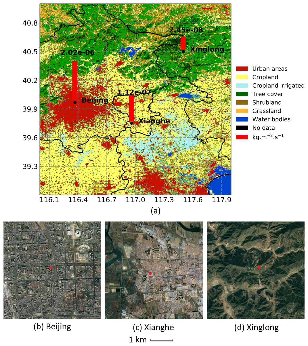
Figure 1(a) The location of three sites at Beijing (BJ, 39.96∘ N, 116.36∘ E; 49 ), Xianghe (XH, 39.75∘ N, 116.96∘ E; 30 ), and Xinglong (XL, 40.40∘ N, 117.50∘ E; 940 ), together with the land cover in this area. The red bars are the carbon dioxide emissions at the three sites based on the EDGAR data. The maps within ∼2 km of (b) BJ, (c) XH, and (d) XL are from © Google Maps (https://www.google.com/maps, last access: 20 July 2021).
It is important to understand atmospheric CO2 variations in urban, suburban, and rural areas. Previous studies carried out in urban areas, such as Phoenix, USA (Idso et al., 2013), and Copenhagen, Denmark (Soegaard and Møller-Jensen, 2003), show that CO2 mole fractions are larger in the city center as compared to the outskirts, which is called the “urban CO2 dome”. Various underlying surfaces, such as buildings, roads, trees, croplands, and grasslands, cause complicated CO2 characteristics (Cheng et al., 2018). George et al. (2007) pointed out that the horizontal gradients of CO2 mole fractions among urban, suburban, and rural areas are caused by different population densities and traffic volumes.
The Beijing–Tianjin–Hebei (BTH) area is an economically dynamic region, located in North China, with highly urbanized cities, suburban cities, and rural areas (Fig. 1). During the last 2 decades, the population in Beijing increased from 13.64 million in 2000 to 21.54 million in 2018, and the number of cars increased from 1.04 million in 2000 to 5.74 million in 2018 (http://data.stats.gov.cn/, last access: 20 July 2021). In the BTH area, the major CO2 emissions come from industry, residential emissions, power plants, and transportation (Song et al., 2013; Feng et al., 2019). In order to reduce the carbon emissions, Beijing has adopted a number of vehicle emission control strategies since the mid-1990s, for example, emission control on new and in-use vehicles, fuel quality improvements, alternative-fuel and advanced vehicles, and public transport (Wu et al., 2011). During China's 12th (2011–2015) and 13th (2016–2020) Five-Year Plan periods, comprehensive work programs were implemented for energy conservation and emission reduction in Beijing. More recently, Beijing also launched the short-term “3-year blue-sky defense battle of Beijing” between 2018 and 2020. Regional networks incorporated with high-accuracy CO2 measurements can be used to retrieve carbon emissions and sinks in the horizontal gradient. The vertical gradient of CO2 mole fractions can also be observed at several different heights at the same location (Bakwin et al., 1998).
To better understand the characteristics of CO2 variations in the BTH area, three cavity ring-down spectroscopy (CRDS) analyzers (Picarro G2301) within 200 km were installed at Beijing (BJ), Xianghe (XH), and Xinglong (XL). The three sites have very different surrounding environments: BJ is inside the megacity, XH is in the suburban area, and XL is in the countryside on a mountain. The measurements between June 2018 and April 2020 at the three sites allow us to better understand the differences among the urban, suburban, and rural sites in relation to the seasonal, synoptic, and diurnal variations of CO2 mole fractions. Section 2 describes the site locations as well as the measurement system. The results and discussions are presented in Sect. 3. Finally, the conclusions are drawn in Sect. 4.
2.1 Sites
The locations of the three sites at BJ (39.96∘ N, 116.36∘ E; 49 ), XH (39.75∘ N, 116.96∘ E; 30 ), and XL (40.40∘ N, 117.50∘ E; 940 ) are shown in Fig. 1. The red bars above the sites are the anthropogenic carbon dioxide emissions in 2015 from the Emission Database for Global Atmospheric Research (EDGAR) v5.0 (Crippa et al., 2019). The CO2 fluxes are , , and at BJ, XH, and XL, respectively.
The BJ site is located in a highly urbanized area, with dense buildings, shopping centers, roads, and residential districts. To the east of the site, there is the Beijing–Tibet expressway (G6), carrying a heavy volume of traffic. Within 1 km of the site, the heights of trees are about 15–20 m, and the heights of buildings are about 70–200 m (Cheng et al., 2018). The vegetation fractions around the BJ site are between 10 % and 18 % (Liu et al., 2012).
The XH site is in a suburban area about 50 km to the southeast of Beijing. XH is surrounded by croplands and irrigated croplands. Within 1 km of the XH site, the residential houses are mainly homebuilt, with an average height of ∼20 m. The center of Xianghe county is about 2 km to the east of the site.
The XL site is located on a mountain, inside the Xinglong Observatory of the National Astronomical Observatories, Chinese Academy of Sciences (NAOC) (https://www.xinglong-naoc.org/html/en/, last access: 20 July 2021), which is about 120 km to the northeast of Beijing. XL is located in a highly vegetated area.
2.2 Measurement system
The Picarro cavity ring-down spectroscopy (CRDS) G2301 analyzers were installed at BJ, XH, and XL to measure CO2, CH4, and H2O mole fractions. The same measurement system is operated at these three sites, which is composed of an intake system, a calibration unit, and a Picarro analyzer (Fig. 2). Note that there are two sampling heights at BJ (80 and 280 ) and XH (60 and 80 ) but only one sampling height (10 ) at XL. The measurements start in June 2018 at BJ and XH and in May 2016 at XL. To compare the CO2 measurements among these sites, we focus on the data after June 2018 in this study.
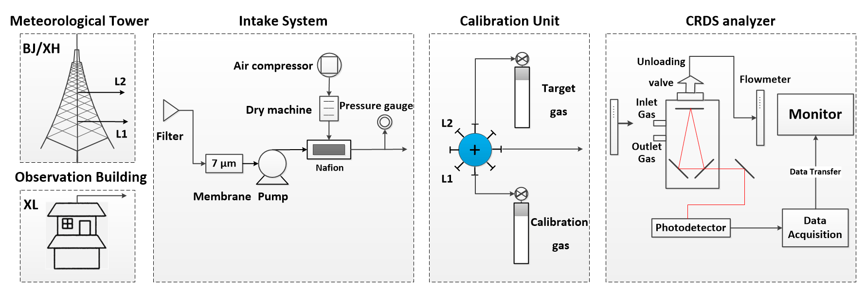
Figure 2Schematic diagram of the measurement system, including a meteorological tower at BJ/XH or observation building at XL, an intake system, a calibration unit, and a CRDS analyzer.
The surrounding air is sampled by a vacuum pump (DA7002D), with a maximum flux of 20 L min−1 through an inlet (Fig. 2). The sample air is then introduced into a 10 mm diameter tube (SYNFLEX 1300), mounted with a capsule filter (Whatman, USA) to filter out solid particles with a diameter larger than 2 µm and liquid particles with a diameter larger than 0.03 mm. In addition, a 7 mm sintered filter (membrane) is installed to filter out solid particles with a diameter larger than 7 µm. Moreover, an air compressor and a dry machine together with a single Nafion tubing selectively permeable membrane dryer (MD-110-72P-4; Perma Pure, Halma, UK) in self-purge are installed to remove water vapor. The sample dew-point temperature can reach down to −25 ∘C, corresponding to a relative humidity of 1 %–20 %. The flux of the Nafion outflow is 200–400 mL min−1. The outflow is then vented to the unloading valve (Fig. 2), which guarantees that the air fed to the Picarro G2301 analyzer is controlled at near-ambient pressure. Before the ambient CO2 measurements, the sampled air is introduced to the calibration unit to check the precision and stability of the system, which will be introduced in detail in Sect. 2.3.
The last part of the measurement system is the Picarro analyzer, which is composed of a laser, a high-finesse optical cavity, and a detector. The sample air is first introduced into the cavity. After that, the laser passes through the sample air, and the intensity of the laser arriving at the detector is monitored as I. Then, the ring-down measurements start as the laser rapidly shuts down. Meanwhile, the sample gas is measured by recording the decay of the laser intensity with time. This decay depends on the optical path inside of the cavity, which is in correlation with the absorption and scattering of the sample air. The analyzer continuously scans the laser over CO2 spectral features and records the absorption loss at a wavelength of 1603 nm to form the spectrum. As a result, CO2 mole fractions are derived from these spectra and collected by the data acquisition part.
2.3 Calibration method
As is shown in Fig. 2, the intake system is connected to an 8-position valve, which is used to choose the air coming from the sample air, the target gas, or the calibration gas. The target and calibration gases are pressurized in 29.5 L treated aluminum alloy cylinders, which are scaled to the WMO X2007 standard by the China Meteorological Administration, Meteorological Observation Center. The same calibration procedure is operated at these three sites: (1) 3 h sample air; (2) 5 min calibration gas; (3) 3 h sample air; and (4) 5 min target gas. This process is repeated every 6 h and 10 min. Note that the air coming from two levels at XH and BJ is switched every 5 min during the 3 h sample air period. As the remaining volume in the tubes needs time for flushing, the response of the analyzer turns to be stable about 1 min after each switching. In order to reduce the uncertainty, we do not consider the first 3 min of measurements after each switching.
The calibration gas is used to calculate the calibration factor (cf) as
where CO2,mcal is the CO2 mole fraction measured by the Picarro analyzer from the calibration gas, and CO2,cal is the standard CO2 mole fraction of the calibration cylinder. The cf is applied to correct the sample air during the next 6 h:
where CO2,m is the CO2 mole fraction measured by the Picarro analyzer, and CO2,c is the calibrated CO2 mole fraction.
The target gas is used to check the precision and stability of the system. The T values are calculated as follows:
where CO2,tar is the standard CO2 mole fraction of the target gas cylinder, and CO2,mtar is the CO2 mole fraction measured by the Picarro analyzer from the target gas.
To keep the CRDS stable over time, only the periods with T values within ±0.1 ppm are selected (Fang et al., 2014). The measurement uncertainties of the Picarro instrument at the three sites are calculated as the standard deviation (SD) of T, which are 0.01, 0.06, and 0.02 ppm at BJ, XH, and XL, respectively.
2.4 Data quality control
Besides the calibration procedure mentioned in Sect. 2.3, we also do auto-flagging and manual flagging of the raw data. In each 1 h CO2 measurement window, auto-flags are assigned when deviations from the CO2 mean are found larger than 2 times the hourly CO2 SD. Furthermore, manual flags are assigned by technicians at each site according to the logbook to exclude invalid data resulted from the inlet filter, pump, and extreme weather issues. In addition, as the CRDS measurement system records CO2 and CH4 simultaneously, the variations of these two gases are checked together to manually flag CO2 and CH4 outliers.
2.5 Meteorological fields
The CO2 variations are additionally characterized by specific meteorological parameters, such as local wind and temperature fields. The meteorological sensors at BJ are installed at the same tower as the Picarro on 120 , and the meteorological sensors at XL are ∼5 m northwest to the Picarro sample tube. The meteorological fields at XH are not discussed here as there is a technical issue with the wind sensor.
Figure 3 shows the wind frequencies at BJ and XL in each season, which are binned with a resolution of 2 m s−1 for the wind speed and 10∘ for the wind direction. At BJ, two dominant wind regimes are observed throughout the whole year: north (northwest to northeast clockwise) and southwest. The percentage of wind frequency in the north region is 34 %, 36 %, 50 %, and 60 %, respectively, from spring to winter. The wind speed varies from 0.63 m s−1 on 10 May 2019 to 14.98 m s−1 on 20 December 2018, with a mean of 3.92 m s−1. From spring to autumn, more winds have a low wind speed. However, in winter, the prevailing northwest wind contributes to high wind frequencies with the increase of wind speed. At XL, the dominant winds are mainly from the west (southwest to northwest clockwise), together with some winds from the southeast. The percentage of wind frequency in the west region is 52 %, 33 %, 56 %, and 57 %, respectively, from spring to winter. The wind speed varies from near-zero on 18 August 2019 to 10.75 m s−1 on 17 April 2019, with a mean of 2.52 m s−1.

Figure 3Wind frequency as a function of wind speed (m s−1) and wind direction (∘) in spring (MAM), summer (JJA), autumn (SON), and winter (DJF) at BJ (a) and XL (b) from October 2018 to September 2019.
The atmospheric boundary layer height (BLH) is another important parameter to characterize the diurnal variation of CO2 (Li et al., 2014; Culf et al., 1997). In this study, we use the BLH hourly data of the ERA5 reanalysis data from the European Centre for Medium-Range Weather Forecasts (ECMWF) with a spatial resolution of (Hersbach et al., 2020).
3.1 CO2 time series and comparison with other urban sites
Figure 4 shows the time series of hourly CO2 mole fractions at the three sites between June 2018 and March 2020. The two-level (80 and 280 m) measurements at BJ are marked as BJ L1 and BJ L2, and the two-level (60 and 80 m) measurements at XH are marked as XH L1 and XH L2. The gaps in the CO2 time series are due to malfunctions of the instruments. To better understand the influence of the wind on CO2, we classify the CO2 mole fractions at XL and BJ L1 based on the wind information into five classes (Fig. 4a and b). The BJ L1 is used here as it is closer to the wind sensor as compared to BJ L2. The local class is defined as wind speed less than 2 m s−1, while wind speeds larger than 2 m s−1 are classified into four sections according to the wind direction: northwest (NW), northeast (NE), southwest (SW), and southeast (SE).
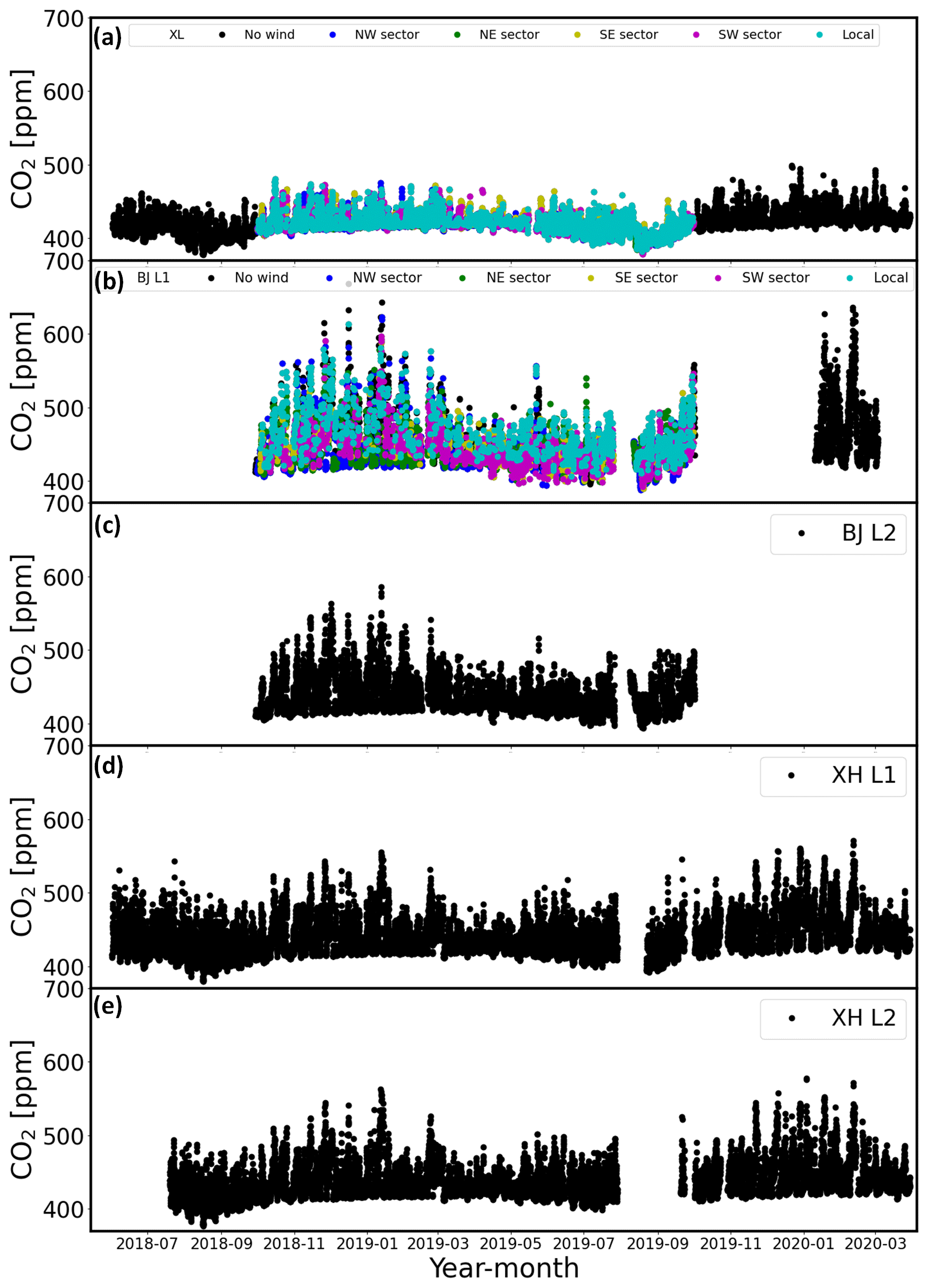
Figure 4The time series of the CO2 measurements at XL (a), BJ L1 (b), BJ L2 (c), XH L1 (d), and XH L2 (e) between June 2018 and March 2020. The CO2 measurements at XL (a) and BJ LI (b) are colored by wind classes discussed in the text.
As expected, the urban BJ site observes a much higher CO2 level than the suburban XH and rural XL sites. The CO2 measurements at the urban site BJ L1 (Fig. 4b) are influenced by the wind speed and wind direction. High CO2 mole fractions generally appear in the local class throughout the whole year, indicating the strong local anthropogenic emissions. The northern sectors (NS and NE) usually contribute low CO2 mole fractions during the autumn–winter period. However, in spring and summer, the SW sector contributes lower CO2, indicating the low CO2 varies with the wind direction by season at BJ. Different from BJ, the CO2 mole fraction in the local class at XL covers the whole data range throughout the whole year. In spring and summer, the wind from the south (SE and SW) makes CO2 increase at XL.
Cheng et al. (2018)Yang et al. (2020)Yang et al. (2019)Sargent et al. (2018)McKain et al. (2015)Lauvaux et al. (2016)Richardson et al. (2017)Verhulst et al. (2017)Mitchell et al. (2018)Bares et al. (2019)Shusterman et al. (2016)Table 1Site characteristics of BJ, XH, and XL in North China and BU, CRA, COM, IMC, and SF in the USA from the CO2 Urban Synthesis and Analysis (CO2-USA) Data Synthesis Network.
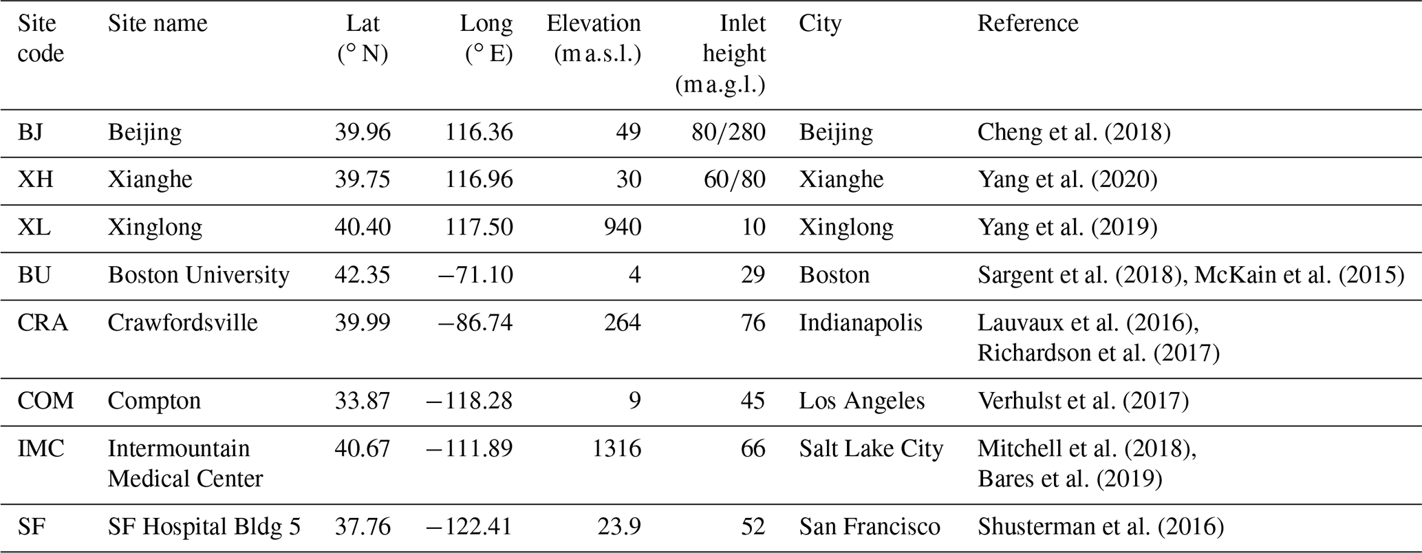
Comparisons with other five urban sites in USA with a similar latitude of BJ are also discussed in this section. All these five sites belong to the CO2 Urban Synthesis and Analysis (CO2-USA) Data Synthesis Network (Feng et al., 2016). The site locations, elevations, inlet heights, and references are listed in Table 1. As the CO2 measurements at these five sites do not cover the period between October 2018 and September 2019, we use the latest 1 year CO2 measurements available. The monthly means and diurnal cycles of CO2 at BJ (L1), XH (L1), and five American urban sites are shown in Fig. 5. It is found that the phases of the seasonal CO2 cycles at BU, CRA, COM, IMC, and SF are consistent with the observations at BJ (L1), XH (L1), and XL, with a high value in autumn–winter and a low value in summer. Among the five American sites, the highest CO2 concentration is observed at IMC. The IMC site is inside a commercial zone, and the CO2 measurements there are more strongly influenced by local emissions (Bares et al., 2019). The CO2 concentration is also high at COM because the Los Angeles megacity is one of the largest fossil fuel CO2 emitters in the world (Matthäus et al., 2021). Figure 5a shows that the CO2 concentrations at COM and IMC are in the same level with the one at XH but are less than the CO2 concentration at BJ. The CO2 concentrations at SF, BU, and CRA are much lower as compared to BJ because of lower anthropogenic emissions at these sites (McKain et al., 2015; Lauvaux et al., 2016; Shusterman et al., 2016).
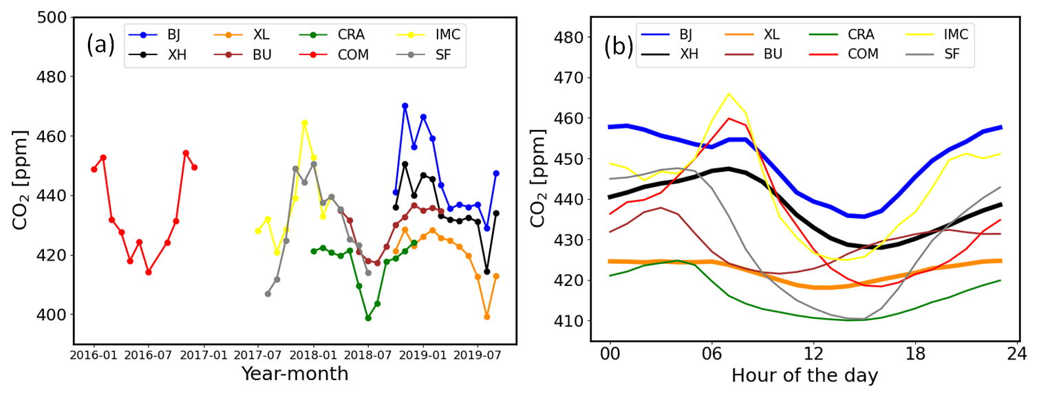
Figure 5(a) Monthly means of CO2 at BJ (L1), XH (L1), and XL between October 2018 and September 2019 and at BU, CRA, COM, IMC, and SF during the latest 1 year and (b) the diurnal cycles of CO2.
Figure 5b shows the diurnal variations of CO2, with the amplitudes of 22.4, 19.4, 6.6, 16.3, 14.8, 41.5, 41.1, and 37.2 ppm at BJ (L1), XH (L1), XL, BU, CRA, COM, IMC, and SF, respectively. The amplitudes of the diurnal variation at COM, IMC, and SF are higher than that at BJ, although the yearly mean CO2 levels at these sites are smaller than that at BJ. As the sampling heights at these sites and BJ are similar, the large amplitudes of the diurnal variation indicate that stronger variation in the local emissions and/or sinks exists at these three American sites as compared to BJ.
3.2 Contribution of main CO2 sources
We use the CarbonTracker model, version CT-NRT.v2021-3 (Peters et al., 2005), to evaluate the influence of anthropogenic, biogenic, oceanic, and fire sources at these three sites, respectively. The CarbonTracker is a data assimilation system developed by the National Oceanic and Atmospheric Administration (NOAA) to keep track of sources and sinks of atmospheric CO2 around the world. Four tracers (biosphere, ocean, fire, and fossil fuel) are treated separately to simulate atmospheric CO2 mole fractions. Mustafa et al. (2020) evaluated the CarbonTracker model in Asia by comparing it with satellite measurements, and they found that the CarbonTracker model captures the variation of CO2 well. The model provides 3-hourly CO2 data at 25 levels from the surface to ∼123 km, and the spatial resolution of the global CarbonTracker CO2 simulation is (longitude × latitude). As BJ and XH are in the same model grid, we note the CO2 simulations in the BJ/XH grid as BJ.
Figure 6 shows the time series of CO2 simulations from fossil fuel (CO2,ff), biosphere (CO2,bio), fire (CO2,fire), and ocean (CO2,oce) modules at BJ/XH and XL between October 2018 and September 2019. It is found that the fire and ocean CO2 at BJ/XH and XL are close to each other throughout the whole year. According to the Global Fire Assimilation System (GFAS) (https://www.ecmwf.int/en/forecasts/dataset/global-fire-assimilation-system/, last access: 20 July 2021) wildfire emissions, there are almost no biomass burning CO2 emissions at BJ, XH, and XL sites. The CarbonTracker model simulations confirm that fire CO2 concentrations in this region are almost the same, and the simulated fire CO2 at these sites is transported by the wildfire emissions in other places. What's more, the CarbonTracker model suggests that the fire CO2 at these sites only takes up a small proportion of the observed CO2 (less than 5 %). The biogenic CO2 at BJ/XH and XL has a similar level between October 2018 and June 2019 and becomes slightly different in summer 2019. However, the difference in biogenic CO2 is much less than that of the anthropogenic CO2 differences. The high CO2 concentrations at BJ and XH in winter are evidently dominated by the enhancement of fossil fuel. The variation of the fossil fuel CO2 at XL is much less than that at BJ/XH. Therefore, using the CO2 measurements at XL as the background, we can significantly reduce the influence from fire, biosphere, and ocean and extract the signal of the anthropogenic CO2 differences.
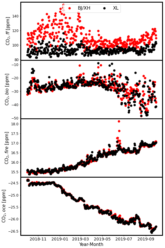
Figure 6The time series of CO2 simulations from fossil fuel (CO2,ff), biosphere (CO2,bio), fire (CO2,fire), and ocean (CO2,oce) modules at BJ/XH and XL.
The CO2 enhancement at BJ or XH relative to XL is then calculated as
The time series of hourly ΔCO2,BJ/XH are presented in Fig. 7a. The ΔCO2 has a maximum in winter and a minimum in summer at both BJ and XH. The high value is probably related to more combustion of fossil fuel from traffic and heating systems in winter (Liu et al., 2012). The daily ΔCO2 can reach up to 106.8 ppm in December 2018 at BJ and 78.5 ppm in January 2019 at XH. The mean ΔCO2 levels at BJ and XH are 26.2±20.6 and 15.2±13.6 ppm, respectively. There are 271 d when ΔCO2 is observed at both BJ and XH (Fig. 7b). The correlation efficiency (R) of 0.81 is found between the Δ CO2 at BJ and XH, indicating that the ΔCO2 levels change simultaneously at BJ and XH. The slope of the linear fitting suggests that the ΔCO2 at BJ is 1.23 times larger than that of XH.
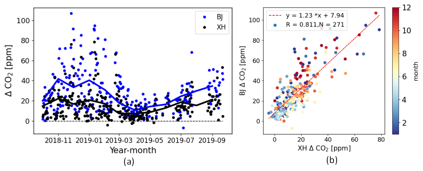
Figure 7(a) The time series of daily CO2 enhancements at BJ and XH relative to XL between October 2018 and September 2019. The blue and black lines are the monthly means of CO2 enhancements at BJ and XH, respectively. (b) The correlation between daily mean CO2 enhancements at BJ and XH.
3.3 Seasonal variations
The seasonal cycles of CO2 are derived from the measurements at the lower levels at BJ and XH and the measurements at XL. The lower levels at BJ and XH are used here as they reflect more information about surface fluxes. Figure 8a shows the CO2 monthly means between October 2018 and September 2019, together with the temperature at BJ and the leaf area index (LAI). The LAI monthly data are from the Copernicus Global Land Service (https://land.copernicus.eu/global/products/lai, last access: 20 July 2021), with a spatial resolution of 1 km. Figure 8a shows the LAI monthly means in the region of Fig. 1.
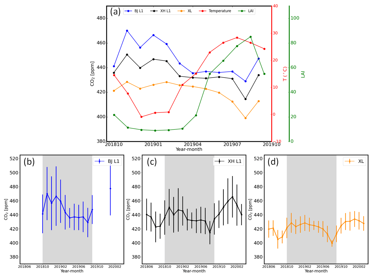
Figure 8(a) The monthly means of CO2 at BJ L1, XH L1, and XL between October 2018 and September 2019. The monthly mean air temperature at BJ and regional mean leaf area index (LAI) of the area in Fig. 1a during the same period are also displayed. (b–d) Monthly means of CO2 together with the 1σ standard deviation at BJ L1, XH L1, and XL between June 2018 and February 2020. The gap at BJ L1 is due to the instrument failure. The shaded area is the measurement period displayed in Fig. 8a.
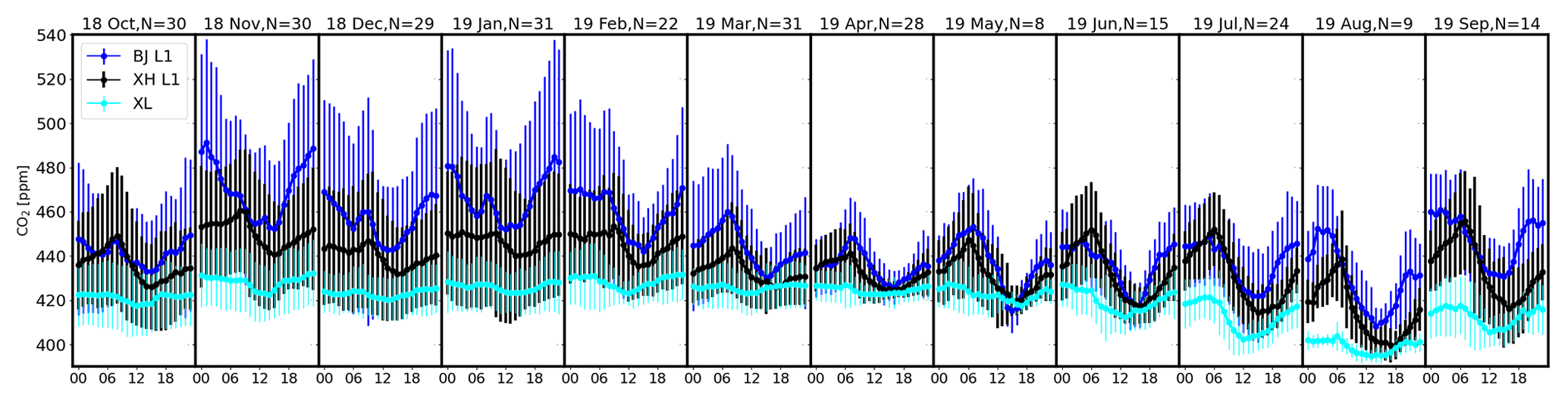
Figure 9The diurnal cycles of CO2 variations at BJ L1, XH L1, and XL in each month between October 2018 and September 2019. The collocated days are displayed (N). The error bars are the hourly standard deviations of CO2.
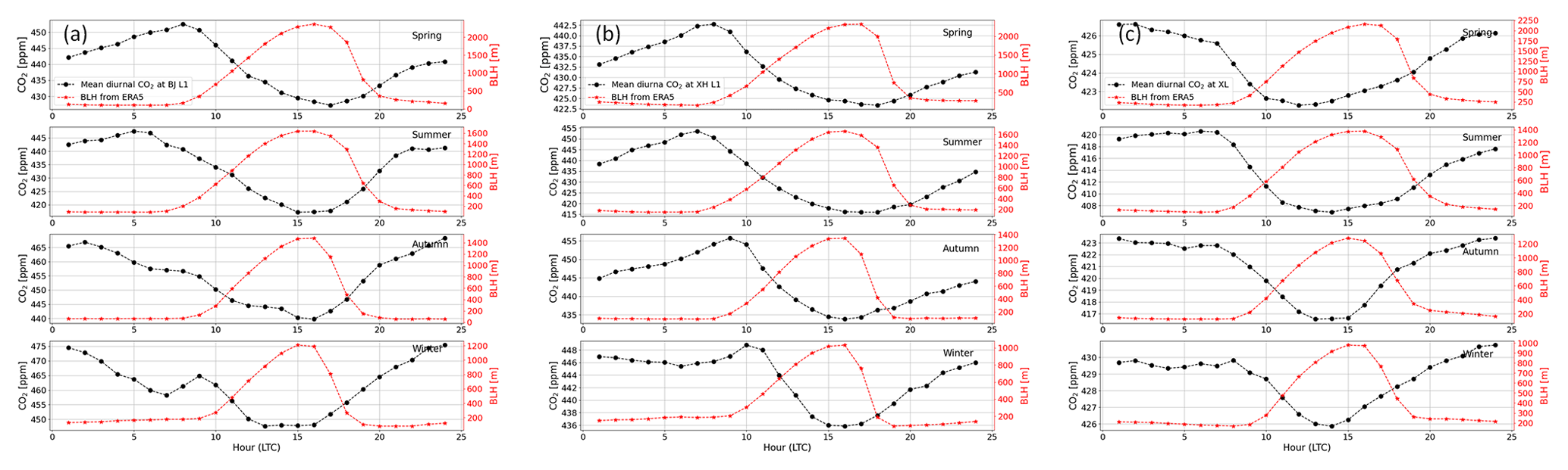
Figure 10(a–c) Mean diurnal cycles of BLH from ERA5 and mean diurnal CO2 variations at BJ L1 (a), XH L1 (b), and XL (c) in each season between October 2018 and September 2019.
Between October 2018 and September 2019, the mean of CO2 mole fractions at BJ is 448.4±12.8 ppm, which is larger than the mean values at XH (436.0±9.2 ppm) and XL (420.6±8.2 ppm). The phases of the seasonal cycle of CO2 at BJ, XH, and XL are similar, with a high value in autumn–winter and a low value in summer, which is consistent with other observations in the Northern Hemisphere (Nevison et al., 2008). This is expected, mainly due to the seasonal cycle of the biosphere fluxes (LAI). The increased temperature in summer is favorable for plant growth, leading to larger photosynthesis. In winter, the respiration of plants and the anthropogenic heating emissions contribute to a high CO2 level. The amplitudes of the seasonal variation of CO2 at BJ, XH, and XL are 41.2, 36.1, and 29.3 ppm, respectively. According to the CarbonTracker simulation (Fig. 6), the CO2 seasonal cycle in this region is mainly driven by the biogenic and anthropogenic CO2. At XL, the anthropogenic CO2 is almost constant through the whole year, while the biogenic CO2 is low in summer and high in winter. For BJ/XH, apart from the similar biogenic CO2 seasonal variation, the anthropogenic CO2 is also high in winter and lower in summer. Therefore, combining the effect from the biosphere and human activities, the amplitude of CO2 seasonal variation at BJ/XH is larger than that at XL. What's more, as the anthropogenic emission at BJ is much larger than that at XH, indicated by the EDGAR emission dataset, we thus observe the largest amplitude of the seasonal variation at BJ.
Figure 8b–d show the CO2 monthly means together with the monthly 1σ standard deviation at each site. We take the days when measurements are available at all three sites or the days when measurements are available at XH and XL. The CO2 variability (1σ) is highest at BJ and lowest at XL. The seasonal CO2 variation and 1σ standard deviation at each site are further assessed in the following.
Autumn. At each site, monthly mean CO2 mole fractions are increasing with the decrease of LAI. The increase rates of CO2 at BJ, XH, and XL are 30, 19, and 9 ppm month−1, respectively. The 1σ standard deviation of each month at BJ is generally larger than that of XH and is then followed by XL.
Winter. The CO2 removed by the photosynthesis is weak in this region as the LAI is low. The CO2 changes simultaneously at BJ and XH, increasing from December 2018 to January 2019 and decreasing afterwards. Similar to autumn, the month-to-month variation of CO2 at BJ is larger than that at BJ and XL, together with the largest 1σ at BJ. The 1σ at BJ and XH is larger in winter as compared to other seasons.
Spring. The decrease of CO2 in March 2019 is highly related to the temperature increase. As the heating is officially stopped in the middle of March, the anthropogenic emissions are much reduced (Shi et al., 2020). In April and May, the LAI increases significantly, leading to the decrease of CO2, especially at XL. The regional biosphere activity affects CO2 mole fractions at XL more, while the large anthropogenic emissions at BJ and XH may reduce the influence from the photosynthesis.
Summer. At all the sites, minimum CO2 is observed in August, with the maximum LAI corresponding to the largest photosynthesis CO2 absorption activity. The month-to-month variation of 1σ is small at BJ and XH.
3.4 Diurnal variations
The diurnal variations of CO2 at BJ, XH, and XL between October 2018 and September 2019 are shown in Fig. 9. The amplitudes of the diurnal variations are between 16.4 and 44.1 ppm at BJ. The relatively large amplitudes are observed in summer and winter compared to spring and autumn. The phase of the diurnal variation at BJ varies with season. There is one peak in the early morning (04:00–07:00) and one trough in the afternoon (14:00–16:00) in spring and summer. However, there are two peaks (08:00–09:00, 22:00–01:00) and two troughs (04:00–07:00, 14:00–16:00) in late autumn and winter. At XH, there is one peak (04:00–07:00) and one trough (14:00–16:00) throughout the whole year. The amplitude of the diurnal variation at XH is about 6–20 ppm smaller than that at BJ between November 2018 and May 2019. At XL, the peak of CO2 occurs around 04:00–07:00, and the trough occurs in the afternoon around 12:00–14:00. The amplitudes of diurnal variations at XL are larger in summer as compared to other seasons. Moreover, the amplitudes of diurnal variations at XL are much smaller as compared to those at BJ and XH, especially in winter.
The diurnal variations of CO2 are mainly affected by the BLH, photosynthesis, and local human activities (Chan et al., 2008; Denning et al., 1999). Generally, the increase of sunlight enhances the plant photosynthetic rate, and vice versa. There is no photosynthetic CO2 sink before sunrise or after sunset (Lv et al., 2020; Bagley et al., 2015). To better understand the influence of the BLH on the diurnal CO2 variations, we show the CO2 diurnal cycles for each season at BJ L1, XH L1, and XL, together with the BLH hourly means (see Fig. 10).
BJ L1. The increase of the BLH after sunrise (05:00–08:00) and the photosynthetic uptake during the day make the CO2 mole fraction decrease. The CO2 mole fraction reaches a minimum in the afternoon around 16:00–17:00, corresponding to the maximum BLH. After that, the BLH decreases, resulting in the accumulation of CO2. In spring and summer, the CO2 mole fraction keeps increasing until the next day (05:00–08:00) before sunrise, and in autumn and winter, the CO2 mole fraction starts decreasing at midnight. Note that the enhancement of CO2 around 09:00 in winter is not related to the BLH, which is probably due to the rush-hour traffic emissions.
XH L1. Similar to BJ, the variation of the CO2 mole fraction is dominated by the BLH during the day. The CO2 mole fraction decreases with the increase of BLH. The CO2 mole fraction reaches a minimum in the afternoon around 16:00–17:00, corresponding to the highest BLH. However, at night, the variation of CO2 at XH is not the same as that at BJ, especially in autumn and winter. In autumn, the CO2 mole fraction keeps increasing until the next day before sunrise (05:00–08:00), and in winter, the CO2 mole fraction stays stable after midnight. Similar to BJ, the peak CO2 around 09:00–10:00 in winter may be due to the traffic emissions in rush hour.
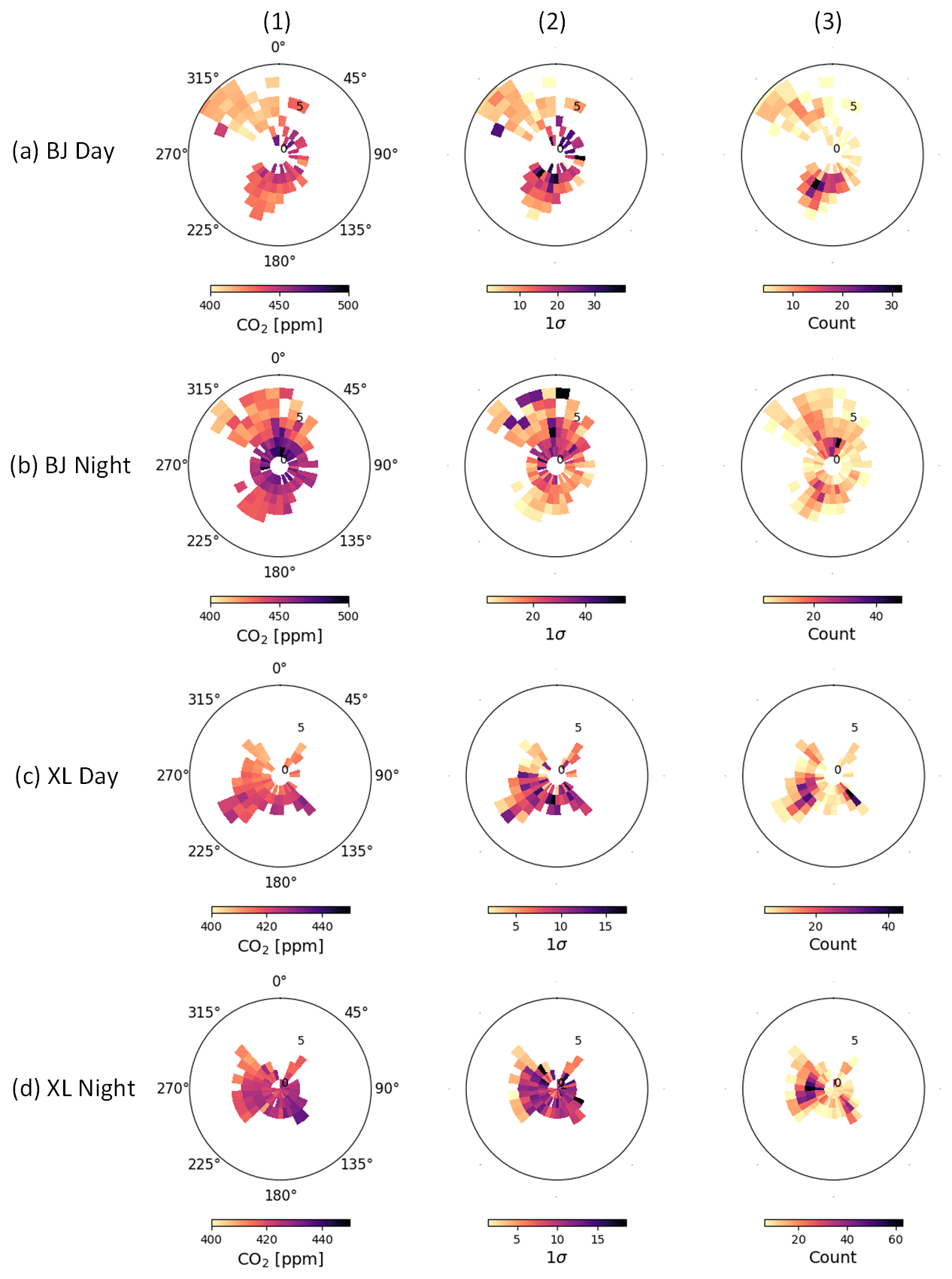
Figure 11(1) Binned CO2 mole fraction as a function of wind speed (m s−1) and wind direction (∘) at BJ L1 (a, b) and XL (c, d) based on daytime (14:00–16:00 LTC) and nighttime (22:00–01:00 LTC) data between October 2018 and September 2019. (2) Mean 1σ standard deviation of the CO2 mole fractions in each bin. (3) The CO2 measurement counts in each bin.
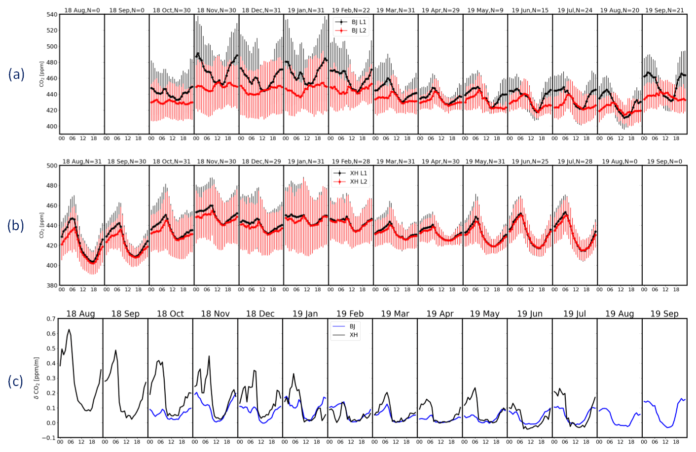
Figure 12(a) The CO2 measurements of BJ L1 and BJ L2 between October 2018 and September 2019. The error bars are the hourly standard deviations of CO2. (b) The CO2 measurements of XH L1 and XH L2 between August 2018 and July 2019. (c) The hourly δCO2 [ppm m−1] in each month at BJ and XH.
XL. Different from BJ and XH, the minimum of the CO2 mole fraction occurs earlier than the maximum of BLH in spring and summer. For example, the minimum of the CO2 mole fraction is around 12:00, and the maximum of BLH occurs around 16:00. The solar radiation is strongest at noon, which leads to the largest rate of photosynthesis removing CO2. The diurnal variation of CO2 at daytime is then strongly affected by the plants in these two seasons. However, in autumn and winter, the minimum of the CO2 mole fraction occurs close to the maximum of the BLH, which is also dominated by the change of the planetary boundary layer (PBL) due to the low LAI in these two seasons (Mohotti and Lawlor, 2002; Newman et al., 2013).
3.5 CO2 variations with the wind
Wind speed and wind direction are the two key factors in modulating the dispersion of CO2 emissions (Turnbull et al., 2015; Lac et al., 2013; Ángeles García et al., 2012). The influence of wind on CO2 mole fraction at BJ and XL is discussed specifically in this section. To minimize the influence from the diurnal variation, we focus on the measurements between 14:00 and 16:00 during daytime for the highest BLH and between 22:00 and 02:00 during nighttime for the lowest BLH. In addition, we reduce the impact from the seasonal variation of CO2 by applying the following method. First, we calculate the mean of CO2 over 10 d (CO2,10 d). Second, the ratio between the CO2,10 d and the annual mean of original CO2 is derived (), and the Indexh is interpolated from the Index10 d at an hourly scale. Finally, the deseasonalized CO2 is calculated as . In summary, we use the deseasonalized CO2 during the daytime (14:00–16:00) and the nighttime (22:00–02:00) separately to understand the influence of the wind.
Figure 11 shows the daytime and nighttime wind roses of CO2 mole fractions at BJ and XL, with a resolution of 1 m s−1 wind speed and 10∘ wind direction. Note that only the bins with the measurement number larger than 3 at BJ or 5 at XL are shown here.
BJ. At BJ, the wind mainly comes from the southwest and the northwest, with more winds coming from the southwest during the day and more winds coming from the northwest at night. The high CO2 mole fractions are observed with a low wind speed (<2 m s−1). For the wind with a relatively large speed (>2 m s−1), it is found that the CO2 with the wind coming from the southwest is about ∼21 ppm larger than that with the wind coming from the northwest during the day.
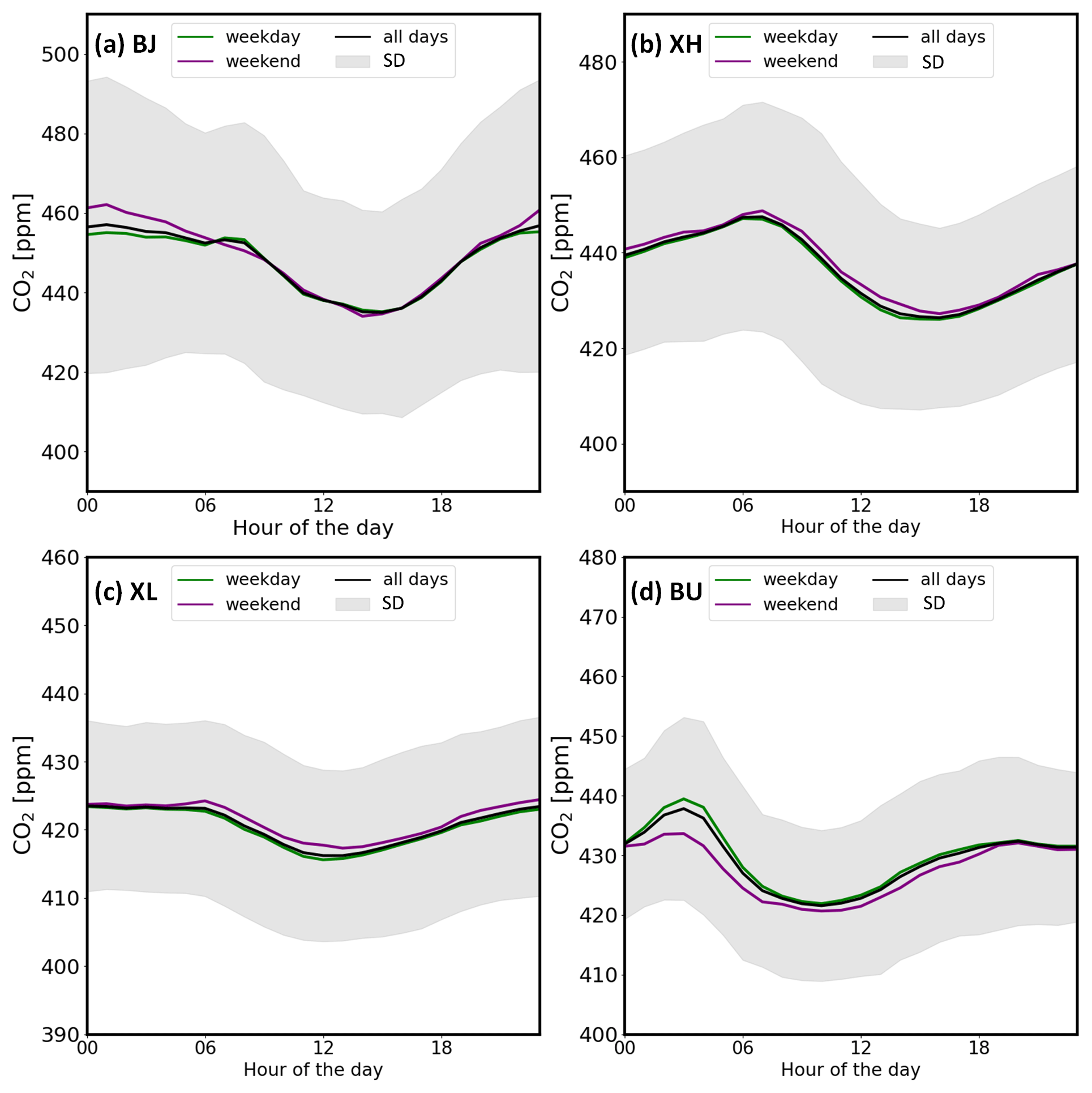
Figure 13 The average hourly means of CO2 on weekdays, weekends, and all days at (a) BJ (L1), (b) XH (L1), (c) XL, and (d) BU (Boston) between October 2018 and September 2019. The light gray shaded area represents 1 standard deviation from the mean for all days.
XL. The wind speed at XL is generally smaller as compared to BJ. The wind at XL is mainly coming from the southeast–northwest sector in a clockwise direction. During the day, the high CO2 mole fractions are observed along with a relatively large wind speed (>2 m s−1). This can be attributed to the impact of remote emissions advocated from the south, where large cities, such as Beijing and Tianjin, are located. At night, although the dominant wind shifts to the west, the high CO2 mole fractions can be observed in almost all the directions, with wind speeds ranging from 0 to 3 m s−1.
3.6 Two-level measurements at BJ and XH
Figure 12 shows the CO2 hourly means observed at two levels at BJ and XH between October 2018 and September 2019. Note that we select measurements when the hourly means are available at both levels.
At BJ, CO2 mole fractions at L1 are generally higher than L2 as L1 is closer to near-ground human emissions. At BJ L1 (80 ), we can observe a peak in the early morning, which corresponds to rush-hour transportation. The trough of CO2 at BJ L1 occurs at 16:00–17:00 because of the maximum PBL resulting from the unstable atmosphere. After that, the atmosphere changes from unstable to stable during the night, leading to the CO2 peak again. At BJ L2 (280 ), the diurnal variation of CO2 generally follows that at L1. Note that the peak of the CO2 at L2 occurs in the early morning, later than that at L1, as the CO2 at the ground level moved upward with the increase in convective PBL, with a large difference in winter and a small difference in summer. The CO2 diurnal variations from two-layer Picarro measurements in 2018 and 2019 in our study are consistent with the seven open-path infrared gas analyzer (Model LI-7500A; at 8, 16, 47, 80, 140, 200, and 280 ) measurements between 2013 and 2016 at the same site (Cheng et al., 2018). In summer, the temperature is high due to a larger solar irradiance; the atmosphere becomes unstable quickly, accelerating the uplifting of the PBL. In winter, the uplifting of the PBL is slow because of the stable atmosphere.
At XH, the CO2 mole fractions at L1 and L2 are closer to each other as compared to the two-layer measurements at BJ because the difference in the vertical distance of the two layers at XH is only 20 m. Nevertheless, we can still observe that the peak of the CO2 at L2 occurs in the early morning, later than that at L1, as the CO2 at the ground level moved upward with the increase in convective PBL, with a large difference in winter and a small difference in summer.
To compare the vertical distribution of CO2 at BJ and XH, we calculate the CO2 gradient () (Fig. 12c). The diurnal variations of δCO2 at BJ and XH have a similar pattern: close to zero during the day and positive at night. The maximum δCO2 can reach up to 0.6 ppm m−1 at XH in August 2018 and 0.2 ppm m−1 at BJ in November 2018. The larger height difference at BJ (120 m) as compared to XH (20 m) may contribute to the smaller δCO2.
3.7 Weekday–weekend variation
Figure 13 shows the average hourly means of CO2 on weekdays, weekends, and all days at BJ (L1), XH (L1), and XL between October 2018 and September 2019 and at BU (Boston) between April 2018 and April 2019. At BJ (L1), the nighttime CO2 measurements on weekends from 20:00 to 06:00 the next morning are generally ∼5 ppm larger than those on weekdays. XH (L1) and XL CO2 measurements on weekends are ∼2 ppm larger than those on weekdays throughout the whole day, respectively. On the contrary, BU CO2 measurements on weekdays are ∼8 ppm larger than those on weekends between 04:00 and 06:00. The CO2 differences on weekday and weekend at BU turn smaller after sunrise. The mean CO2 at BJ (L1), XH (L1), XL, and BU is 447.6, 436.2, 420.3, and 429.8 ppm, respectively, on weekdays and 449.2, 437.6, 421.4, and 427.5 ppm, respectively, on weekends. The weekday–weekend variations at BJ and XH are similar to those at Nanjing, China (Gao et al., 2018), where CO2 mole fractions are higher at the weekends but different from Boston, USA, London, UK, and Tamil Nadu, India, where the CO2 mole fractions are higher on weekday (Hernández-Paniagua et al., 2015; Kishore Kumar and Shiva Nagendra, 2015; Briber et al., 2013).
In this study, we show the CO2 measurements from the in situ Picarro instruments at BJ, XH, and XL between June 2018 and March 2020. It is the first time that CO2 variations at these sites are investigated. BJ is inside the megacity, XH is in the suburban area, and XL is in the countryside on a mountain. The uncertainties of the CO2 are 0.01, 0.06, and 0.02 ppm at BJ, XH, and XL, respectively. The means and SDs of CO2 mole fractions are 448.4±12.8, 436.0±9.2, and 420.6±8.2 ppm at BJ (L1), XH (L1), and XL, respectively. The CarbonTracker simulations at these three sites show that fire, ocean, and biogenic CO2 levels are close to each other throughout the whole year, and the variation of the fossil fuel CO2 at XL is much less than that at BJ/XH. The CO2 measurements at XL are used to represent the background, and we find that there is a good relationship between the CO2 enhancements at BJ and XH. BJ and XH are affected by CO2 emissions and transport simultaneously. Comparison with other urban sites in the USA shows that the CO2 concentration is the largest at BJ.
The variations of CO2 at BJ, XH, and XL are discussed on diurnal and seasonal scales. It is found that the seasonal cycles of CO2 at these three sites are similar, with a high value in winter and a low value in summer, which is closely related to air temperature and LAI. However, the amplitudes of seasonal variations are different, with the values of 41.2, 36.1, and 29.3 ppm at BJ, XH, and XL, respectively. For the diurnal variation, the CO2 is relatively low during the day and high at night. The diurnal variation of CO2 at BJ, XH, and XL is affected by the BLH, photosynthesis, and human activities, and the impact of photosynthesis is more significant at XL.
The CO2 measurements are compared against the local wind data at BJ and XL. At BJ, high CO2 mole fractions are observed with low wind speeds (<2 m s−1). At XL, the high CO2 mole fractions during daytime are observed with the wind coming from the south, where the urban area is located.
The two-level measurements at BJ and XH show that the CO2 mole fractions at lower and upper levels are close to each other during the day. The CO2 mole fraction at the lower level is larger than that at the upper level at night, with a vertical gradient of up to 0.6 ppm m−1 at XH and 0.2 ppb m−1 at BJ. The CO2 mole fractions on weekends at BJ, XH, and XL are found to be slightly higher than the ones on weekdays.
The Carbon-Tracker model data are publicly available at https://doi.org/10.25925/ED7S-M661 (last access: 20 July 2021) (Jacobson et al., 2021). The ERA5 reanalysis data are publicly available at https://doi.org/10.24381/cds.adbb2d47 (last access: 20 July 2021) (Hersbach et al., 2018). The CO2 measurements at Beijing, Xianghe, and Xinglong are available upon request to the authors.
MZ, TW, PW, and GW designed the experiment. YY performed the data curation. YY and MZ wrote the paper, and all authors read and provided comments on the paper.
The authors declare that they have no conflict of interest.
Publisher's note: Copernicus Publications remains neutral with regard to jurisdictional claims in published maps and institutional affiliations.
We want to thank Weidong Nan, Qun Cheng, and Qing Yao, at the Xianghe site, Wenhai Chai, at the Xinglong site, and the staff, at the Beijing site, for the Picarro maintenance.
This research has been supported by the National Natural Science Foundation of China (grant no. 41575034), the National Key R & D Program of China (grant nos. 2017YFC1501701, 2017YFB0504000, and 2017YFC1501902), and the Science and Technology Commission of the Shanghai Municipality (grant nos. 19DZ1200103 and 17DZ1205300).
This paper was edited by Eduardo Landulfo and reviewed by three anonymous referees.
Ángeles García, M., Sánchez, M. L., and Pérez, I. A.: Differences between carbon dioxide levels over suburban and rural sites in Northern Spain, Environ. Sci. Pollut. R., 19, 432–439, https://doi.org/10.1007/s11356-011-0575-4, 2012. a
Bagley, J., Rosenthal, D. M., Ruiz-Vera, U. M., Siebers, M. H., Kumar, P., Ort, D. R., and Bernacchi, C. J.: The influence of photosynthetic acclimation to rising CO2 and warmer temperatures on leaf and canopy photosynthesis models, Global Biogeochem. Cy., 29, 194–206, https://doi.org/10.1002/2014GB004848, 2015. a
Bakwin, P. S., Tans, P. P., Hurst, D. F., and Zhao, C.: Measurements of carbon dioxide on very tall towers: results of the NOAA/CMDL program, Tellus B, 50, 401–415, https://doi.org/10.1034/j.1600-0889.1998.t01-4-00001.x, 1998. a
Bares, R., Mitchell, L., Fasoli, B., Bowling, D. R., Catharine, D., Garcia, M., Eng, B., Ehleringer, J., and Lin, J. C.: The Utah urban carbon dioxide (UUCON) and Uintah Basin greenhouse gas networks: instrumentation, data, and measurement uncertainty, Earth Syst. Sci. Data, 11, 1291–1308, https://doi.org/10.5194/essd-11-1291-2019, 2019. a, b
Briber, B. M., Hutyra, L. R., Dunn, A. L., Raciti, S. M., and Munger, J. W.: Variations in Atmospheric CO2 Mixing Ratios across a Boston, MA Urban to Rural Gradient, Land, 2, 304–327, https://doi.org/10.3390/land2030304, 2013. a
Chan, D., Ishizawa, M., Higuchi, K., Maksyutov, S., and Chen, J.: Seasonal CO2 rectifier effect and large-scale extratropical atmospheric transport, J. Geophys. Res., 113, D17309, https://doi.org/10.1029/2007JD009443, 2008. a
Cheng, X. L., Liu, X. M., Liu, Y. J., and Hu, F.: Characteristics of CO2 Concentration and Flux in the Beijing Urban Area, J. Geophys. Res.-Atmos., 123, 1785–1801, https://doi.org/10.1002/2017JD027409, 2018. a, b, c, d
Churkina, G.: The role of urbanization in the global carbon cycle, Front. Ecol. Evol., 3, 144, https://doi.org/10.3389/fevo.2015.00144, 2016. a
Crippa, M., Oreggioni, G., Guizzardi, D., Muntean, M., Schaaf, E., Vullo, E. L., Solazzo, E., Monforti-Ferrario, F., Olivier, J., and Vignati, E.: Fossil CO2 and GHG emissions of all world countries – 2019 Report, Publications Office of the European Union, Luxembourg, ISBN 978-92-76-11100-9, https://doi.org/10.2760/687800, 2019. a
Culf, A., Fisch, G., Malhi, Y., and Nobre, C.: The influence of the atmospheric boundary layer on carbon dioxide concentrations over a tropical forest, Agr. Forest Meteorol., 85, 149–158, https://doi.org/10.1016/S0168-1923(96)02412-4, 1997. a
Denning, A. S., Takahashi, T., and Friedlingstein, P.: Can a strong atmospheric CO2 rectifier effect be reconciled with a “reasonable” carbon budget?, Tellus B, 51, 249–253, https://doi.org/10.1034/j.1600-0889.1999.t01-1-00010.x, 1999. a
Dhakal, S.: Urban energy use and carbon emissions from cities in China and policy implications, Energ. Policy, 37, 4208–4219, https://doi.org/10.1016/j.enpol.2009.05.020, 2009. a
Fang, S. X., Zhou, L. X., Tans, P. P., Ciais, P., Steinbacher, M., Xu, L., and Luan, T.: In situ measurement of atmospheric CO2 at the four WMO/GAW stations in China, Atmos. Chem. Phys., 14, 2541–2554, https://doi.org/10.5194/acp-14-2541-2014, 2014. a
Feng, S., Lauvaux, T., Newman, S., Rao, P., Ahmadov, R., Deng, A., Díaz-Isaac, L. I., Duren, R. M., Fischer, M. L., Gerbig, C., Gurney, K. R., Huang, J., Jeong, S., Li, Z., Miller, C. E., O'Keeffe, D., Patarasuk, R., Sander, S. P., Song, Y., Wong, K. W., and Yung, Y. L.: Los Angeles megacity: a high-resolution land–atmosphere modelling system for urban CO2 emissions, Atmos. Chem. Phys., 16, 9019–9045, https://doi.org/10.5194/acp-16-9019-2016, 2016. a
Feng, T., Zhou, W., Wu, S., Niu, Z., Cheng, P., Xiong, X., and Li, G.: High-resolution simulation of wintertime fossil fuel CO2 in Beijing, China: Characteristics, sources, and regional transport, Atmos. Environ., 198, 226–235, https://doi.org/10.1016/j.atmosenv.2018.10.054, 2019. a
Gao, Y. Q., Lee, X. H., Liu, S. D., Hu, N., Wei, X., Hu, C., Liu, C., Zhang, Z., and Yang, Y. C.: Spatio-temporal variability of the near-surface CO2 concentration across an industrial-urban-rural transect, Nanjing, China, Sci. Total Environ., 631–632, 1192–1200, https://doi.org/10.1016/j.scitotenv.2018.03.126, 2018. a, b
George, K., Ziska, L., Bunce, J., and Quebedeaux, B.: Elevated atmospheric CO2 concentration and temperature across an urban-rural transect, Atmos. Environ., 41, 7654–7665, https://doi.org/10.1016/j.atmosenv.2007.08.018, 2007. a
Hansen, J., Sato, M., Kharecha, P., and von Schuckmann, K.: Earth's energy imbalance and implications, Atmos. Chem. Phys., 11, 13421–13449, https://doi.org/10.5194/acp-11-13421-2011, 2011. a
Hernández-Paniagua, I. Y., Lowry, D., Clemitshaw, K. C., Fisher, R. E., France, J. L., Lanoisellé, M., Ramonet, M., and Nisbet, E. G.: Diurnal, seasonal, and annual trends in atmospheric CO2 at southwest London during 2000–2012: Wind sector analysis and comparison with Mace Head, Ireland, Atmos. Environ., 105, 138–147, https://doi.org/10.1016/j.atmosenv.2015.01.021, 2015. a
Hersbach, H., Bell, B., Berrisford, P., Biavati, G., Horányi, A., Muñoz Sabater, J., Nicolas, J., Peubey, C., Radu, R., Rozum, I., Schepers, D., Simmons, A., Soci, C., Dee, D., and Thépaut, J.-N.: ERA5 hourly data on single levels from 1979 to present, Copernicus Climate Change Service (C3S) Climate Data Store (CDS) [data set], https://doi.org/10.24381/cds.adbb2d47, 2018. a
Hersbach, H., Bell, B., Berrisford, P., Hirahara, S., Horányi, A., Muñoz-Sabater, J., Nicolas, J., Peubey, C., Radu, R., Schepers, D., Simmons, A., Soci, C., Abdalla, S., Abellan, X., Balsamo, G., Bechtold, P., Biavati, G., Bidlot, J., Bonavita, M., De Chiara, G., Dahlgren, P., Dee, D., Diamantakis, M., Dragani, R., Flemming, J., Forbes, R., Fuentes, M., Geer, A., Haimberger, L., Healy, S., Hogan, R. J., Hólm, E., Janisková, M., Keeley, S., Laloyaux, P., Lopez, P., Lupu, C., Radnoti, G., de Rosnay, P., Rozum, I., Vamborg, F., Villaume, S., and Thépaut, J.-N.: The ERA5 global reanalysis, Q. J. Roy. Meteor. Soc., 146, 1999–2049, https://doi.org/10.1002/qj.3803, 2020. a
Idso, C., Idso, S., and Balling, R.: The urban CO2 dome of Phoenix, Arizona, Phys. Geogr., 19, 95–108, https://doi.org/10.1080/02723646.1998.10642642, 2013. a
IPCC: Climate change 2013: The physical science basis, Contribution of Working Group I to the Fifth Assessment Report of the Intergovernmental Panel on Climate Change, Cambridge University Press, Cambridge, available at: https://www.ipcc.ch/report/ar5/wg1/ (last access: 20 July 2021), 2013. a
Jacobson, A. R., Schuldt, K. N., Miller, J. B., Tans, P., Arlyn, A., Mund, J., Aalto, T., Abshire, J. B., Aikin, K., Aoki, S., Apadula, F., Baier, B., Bakwin, P., Bartyzel, J., Bentz, G., Bergamaschi, P., Beyersdorf, A., Biermann, T., Biraud, S. C. et al.: CarbonTracker Near-Real Time, CT-NRT.v2021-3, NOAA Earth System Research Laboratory, Global Monitoring Division [data set], https://doi.org/10.25925/ED7S-M661, 2021. a
Kishore Kumar, M. and Shiva Nagendra, S.: Characteristics of ground level CO2 concentrations over contrasting land uses in a tropical urban environment, Atmos. Environ., 115, 286–294, https://doi.org/10.1016/j.atmosenv.2015.05.044, 2015. a
Lac, C., Donnelly, R. P., Masson, V., Pal, S., Riette, S., Donier, S., Queguiner, S., Tanguy, G., Ammoura, L., and Xueref-Remy, I.: CO2 dispersion modelling over Paris region within the CO2-MEGAPARIS project, Atmos. Chem. Phys., 13, 4941–4961, https://doi.org/10.5194/acp-13-4941-2013, 2013. a
Lauvaux, T., Miles, N. L., Deng, A., Richardson, S. J., Cambaliza, M. O., Davis, K. J., Gaudet, B., Gurney, K. R., Huang, J., O'Keefe, D., Song, Y., Karion, A., Oda, T., Patarasuk, R., Razlivanov, I., Sarmiento, D., Shepson, P., Sweeney, C., Turnbull, J., and Wu, K.: High-resolution atmospheric inversion of urban CO2 emissions during the dormant season of the Indianapolis Flux Experiment (INFLUX), J. Geophys. Res.-Atmos., 121, 5213–5236, https://doi.org/10.1002/2015JD024473, 2016. a, b
Li, Y., Deng, J., Mu, C., Xing, Z., and Du, K.: Vertical distribution of CO2 in the atmospheric boundary layer: Characteristics and impact of meteorological variables, Atmos. Environ., 91, 110–117, https://doi.org/10.1016/j.atmosenv.2014.03.067, 2014. a
Liu, H. Z., Feng, J. W., Järvi, L., and Vesala, T.: Four-year (2006–2009) eddy covariance measurements of CO2 flux over an urban area in Beijing, Atmos. Chem. Phys., 12, 7881–7892, https://doi.org/10.5194/acp-12-7881-2012, 2012. a, b
Lv, Z., Shi, Y., Zang, S., and Sun, L.: Spatial and Temporal Variations of Atmospheric CO2 Concentration in China and Its Influencing Factors, Atmosphere, 11, 231, https://doi.org/10.3390/atmos11030231, 2020. a
Matthäus, K., Annmarie, E., Dustin, R., Lin, J., Feng, S., Lei, R. X., Lauvaux, T., Oda, T., Roehl, C., Blavier, J. F., and Iraci, L.: Urban-focused satellite CO2 observations from the Orbiting Carbon Observatory-3: A first look at the Los Angeles megacity, Remote Sens. Environ., 258, 112314, https://doi.org/10.1016/j.rse.2021.112314, 2021. a
McKain, K., Down, A., Raciti, S. M., Budney, J., Hutyra, L. R., Floerchinger, C., Herndon, S. C., Nehrkorn, T., Zahniser, M. S., Jackson, R. B., Phillips, N., and Wofsy, S. C.: Methane emissions from natural gas infrastructure and use in the urban region of Boston, Massachusetts, P. Natl. Acad. Sci. USA, 112, 1941–1946, https://doi.org/10.1073/pnas.1416261112, 2015. a, b
Mitchell, L. E., Lin, J. C., Bowling, D. R., Pataki, D. E., Strong, C., Schauer, A. J., Bares, R., Bush, S. E., Stephens, B. B., Mendoza, D., Mallia, D., Holland, L., Gurney, K. R., and Ehleringer, J. R.: Long-term urban carbon dioxide observations reveal spatial and temporal dynamics related to urban characteristics and growth, P. Natl. Acad. Sci. USA, 115, 2912–2917, https://doi.org/10.1073/pnas.1702393115, 2018. a
Mohotti, A. J. and Lawlor, D. W.: Diurnal variation of photosynthesis and photoinhibition in tea: effects of irradiance and nitrogen supply during growth in the field, J. Exp. Bot., 53, 313–322, 2002. a
Mustafa, F., Bu, L. B., Wang, Q., Ali, M. A., Bilal, M., Shahzaman, M., and Qiu, Z. F.: Multi-Year Comparison of CO2 Concentration from NOAA Carbon Tracker Reanalysis Model with Data from GOSAT and OCO-2 over Asia, Remote Sens.-Basel, 12, 2498, https://doi.org/10.3390/rs12152498, 2020. a
Nevison, C. D., Mahowald, N. M., Doney, S. C., Lima, I. D., Werf, G. R. V. D., Randerson, J. T., Baker, D. F., And, P. K., and Mckinley, G. A.: Contribution of ocean, fossil fuel, land biosphere, and biomass burning carbon fluxes to seasonal and interannual variability in atmospheric CO2, J. Geophys. Res., 113, G01010, https://doi.org/10.1029/2007JG000408, 2008. a
Newman, S., Jeong, S., Fischer, M. L., Xu, X., Haman, C. L., Lefer, B., Alvarez, S., Rappenglueck, B., Kort, E. A., Andrews, A. E., Peischl, J., Gurney, K. R., Miller, C. E., and Yung, Y. L.: Diurnal tracking of anthropogenic CO2 emissions in the Los Angeles basin megacity during spring 2010, Atmos. Chem. Phys., 13, 4359–4372, https://doi.org/10.5194/acp-13-4359-2013, 2013. a
Peters, W., Miller, J. B., Whitaker, J., Denning, A. S., Hirsch, A., Krol, M. C., Zupanski, D., Bruhwiler, L., and Tans, P. P.: An ensemble data assimilation system to estimate CO2 surface fluxes from atmospheric trace gas observations, J. Geophys. Res., 110, D24304, https://doi.org/10.1029/2005JD006157, 2005. a
Richardson, S., Miles, N., Davis, K. J., Lauvaux, T., Martins, D. K., Turnbull, J. C., McKain, K., Sweeney, C., and Cambaliza, M. O. L.: Tower measurement network of in-situ CO2, CH4, and CO in support of the Indianapolis FLUX (INFLUX) Experiment, Elementa: Science of the Anthropocene, 5, 59, https://doi.org/10.1525/elementa.140, 2017. a
Sargent, M., Barrera, Y., Nehrkorn, T., Hutyra, L. R., Gately, C. K., Jones, T., McKain, K., Sweeney, C., Hegarty, J., Hardiman, B., Wang, J. A., and Wofsy, S. C.: Anthropogenic and biogenic CO2 fluxes in the Boston urban region, P. Natl. Acad. Sci. USA, 115, 7491–7496, https://doi.org/10.1073/pnas.1803715115, 2018. a
Shi, Y., Xi, Z., Simayi, M., Li, J., and Xie, S.: Scattered coal is the largest source of ambient volatile organic compounds during the heating season in Beijing, Atmos. Chem. Phys., 20, 9351–9369, https://doi.org/10.5194/acp-20-9351-2020, 2020. a
Shusterman, A. A., Teige, V. E., Turner, A. J., Newman, C., Kim, J., and Cohen, R. C.: The BErkeley Atmospheric CO2 Observation Network: initial evaluation, Atmos. Chem. Phys., 16, 13449–13463, https://doi.org/10.5194/acp-16-13449-2016, 2016. a, b
Soegaard, H. and Møller-Jensen, L.: Towards a spatial CO2 budget of a metropolitan region based on textural image classification and flux measurements, Remote Sens. Environ., 87, 283–294, https://doi.org/10.1016/S0034-4257(03)00185-8, 2003. a
Song, T., Wang, Y., and Sun, Y.: Estimation of carbon dioxide flux and source partitioning over Beijing, China, J. Environ. Sci., 25, 2429–2434, https://doi.org/10.1016/S1001-0742(12)60336-2, 2013. a
Turnbull, J. C., Sweeney, C., Karion, A., Newberger, T., Lehman, S. J., Tans, P. P., Davis, K. J., Lauvaux, T., Miles, N. L., Richardson, S. J., Cambaliza, M. O., Shepson, P. B., Gurney, K., Patarasuk, R., and Razlivanov, I.: Toward quantification and source sector identification of fossil fuel CO2 emissions from an urban area: Results from the INFLUX experiment, J. Geophys. Res.-Atmos., 120, 292–312, https://doi.org/10.1002/2014JD022555, 2015. a
Verhulst, K. R., Karion, A., Kim, J., Salameh, P. K., Keeling, R. F., Newman, S., Miller, J., Sloop, C., Pongetti, T., Rao, P., Wong, C., Hopkins, F. M., Yadav, V., Weiss, R. F., Duren, R. M., and Miller, C. E.: Carbon dioxide and methane measurements from the Los Angeles Megacity Carbon Project – Part 1: calibration, urban enhancements, and uncertainty estimates, Atmos. Chem. Phys., 17, 8313–8341, https://doi.org/10.5194/acp-17-8313-2017, 2017. a
Wu, Y., Wang, R., Zhou, Y., Lin, B., Fu, L., He, K., and Hao, J.: On-Road Vehicle Emission Control in Beijing: Past, Present, and Future, Environ. Sci. Technol., 45, 147–153, https://doi.org/10.1021/es1014289, 2011. a
Yang, Y., Wang, T., Wang, P. C., Zhou, M. Q., and Yao, B.: In-situ measurement of CO2 at the Xinglong regional background station over North China, Atmospheric and Oceanic Science Letters, 12, 385–391, https://doi.org/10.1080/16742834.2019.1644949, 2019. a
Yang, Y., Zhou, M., Langerock, B., Sha, M. K., Hermans, C., Wang, T., Ji, D., Vigouroux, C., Kumps, N., Wang, G., De Mazière, M., and Wang, P.: New ground-based Fourier-transform near-infrared solar absorption measurements of XCO2, XCH4 and XCO at Xianghe, China, Earth Syst. Sci. Data, 12, 1679–1696, https://doi.org/10.5194/essd-12-1679-2020, 2020. a