the Creative Commons Attribution 4.0 License.
the Creative Commons Attribution 4.0 License.
 | 27 Jan 2021
Evidence for the predictability of changes in the stratospheric aerosol size following volcanic eruptions of diverse magnitudes using space-based instruments
Mahesh Kovilakam
Anja Schmidt
Christian von Savigny
Travis Knepp
Landon Rieger
An analysis of multiwavelength stratospheric aerosol extinction coefficient data from the Stratospheric Aerosol and Gas Experiment II and III/ISS instruments is used to demonstrate a coherent relationship between the perturbation in extinction coefficient in an eruption's main aerosol layer and the wavelength dependence of that perturbation. This relationship spans multiple orders of magnitude in the aerosol extinction coefficient of stratospheric impact of volcanic events. The relationship is measurement-based and does not rely on assumptions about the aerosol size distribution. We note limitations on this analysis including that the presence of significant amounts of ash in the main sulfuric acid aerosol layer and other factors may significantly modulate these results. Despite these limitations, the findings suggest an avenue for improving aerosol extinction coefficient measurements from single-channel observations such as the Optical Spectrograph and Infrared Imager System as they rely on a prior assumptions about particle size. They may also represent a distinct avenue for the comparison of observations with interactive aerosol models used in global climate models and Earth system models.
- Article
(5542 KB) - Full-text XML
- BibTeX
- EndNote


Volcanic eruptions represent the primary source of variation in stratospheric aerosol levels (Thomason et al., 1997b; Solomon et al., 2011; Schmidt et al., 2018; Robock, 2000). The optical signature of volcanically derived aerosol is generally dominated by sulfuric acid droplets, but this can be enhanced by the presence of ash either mixed with the sulfuric acid droplets or as distinct layers (Winker and Osborn, 1992; Vernier et al., 2016). Sulfuric acid aerosol is known for its ability to significantly modulate climate (Schmidt and Robock, 2015), primarily by scattering incoming solar radiation to space, and even relatively small volcanic events have been noted to affect global temperature trends (Santer et al., 2014). In addition, as sulfuric acid aerosol particles absorb upwelling infrared radiation, the presence of a volcanic aerosol layer can change the thermal structure of the stratosphere (Labitzke, 1994) and the troposphere and modulate stratospheric circulation as well as transport across the tropopause (Pitari et al., 2016). Significant effort has been expended toward measuring stratospheric aerosol using a variety of instruments (Kremser et al., 2016), and an extensive data collection of observations are now available. Some global climate models (GCMs) and Earth system models (ESMs) use these measurements or parameters directly derived from them (Mann et al., 2015), whereas others, which use interactive aerosol model schemes (Mills et al., 2016) and similar tools (Toohey et al., 2016), assess how well their tools replicate observations and, thus, infer the reliability of the models' assessment of the climate impact of volcanic eruptions (Timmreck et al., 2016).
The initial impetus for this study was to develop tools to understand how reliably the long-term variability of stratospheric aerosol can be characterized given the limited data sets available. Thus, one aim of this work was to understand how small to moderate volcanic events manifest themselves in SAGE II/III observations with the goal of inferring the uncertainty in single-wavelength space-based data sets that use a fixed aerosol size distribution as a part of their retrieval algorithm, such as the Optical Spectrograph and Infrared Imager System (OSIRIS; 2002–present) and the Cloud-Aerosol LIdar with Orthogonal Polarization (CALIOP; 2006–present) (Rieger et al., 2019; Kar et al., 2019). The current OSIRIS algorithm is dependent on a priori assumptions about the aerosol size distribution and, thus, a fixed spectral dependence for aerosol extinction coefficient. As we show below, there are substantial changes in the spectral dependence of aerosol extinction coefficient following these eruptions, which the current OSIRIS algorithm does not capture. A longer-term goal is to infer how well the wavelength dependence can be estimated for these single-wavelength measurements. These factors are relevant not only for understanding the limitations in single-channel data sets but also for the multi-instrument data sets that are reliant on them, such as the Global Space-based Stratospheric Aerosol Climatology (GloSSAC) (Kovilakam et al., 2020).
For this study, we make use of observations made by the Stratospheric Aerosol and Gas Experiment (SAGE) II (1984–2005) and III/ISS (2017–present) which span a broad range of volcanic perturbations of the stratosphere. We demonstrate that, for the most part, the changes in aerosol extinction coefficient and apparent aerosol particle size, where we use the spectral dependence of aerosol extinction coefficient as a proxy for size, are well correlated across nearly 2 orders of magnitude in extinction coefficient change. This relationship is a directly measurable characteristic of the changes in the aerosol size distribution following an eruption without assumptions regarding the functional form for the aerosol size distribution (e.g., lognormal). As comparisons of interactive aerosol model scheme calculations and measurements of stratospheric aerosol form the basis of assessing how well GCMs' and ESMs' microphysics modules perform, the observed relationship provides a potentially unique, measurement-focused means of assessing interactive aerosol models for volcanic eruptions of different magnitudes.
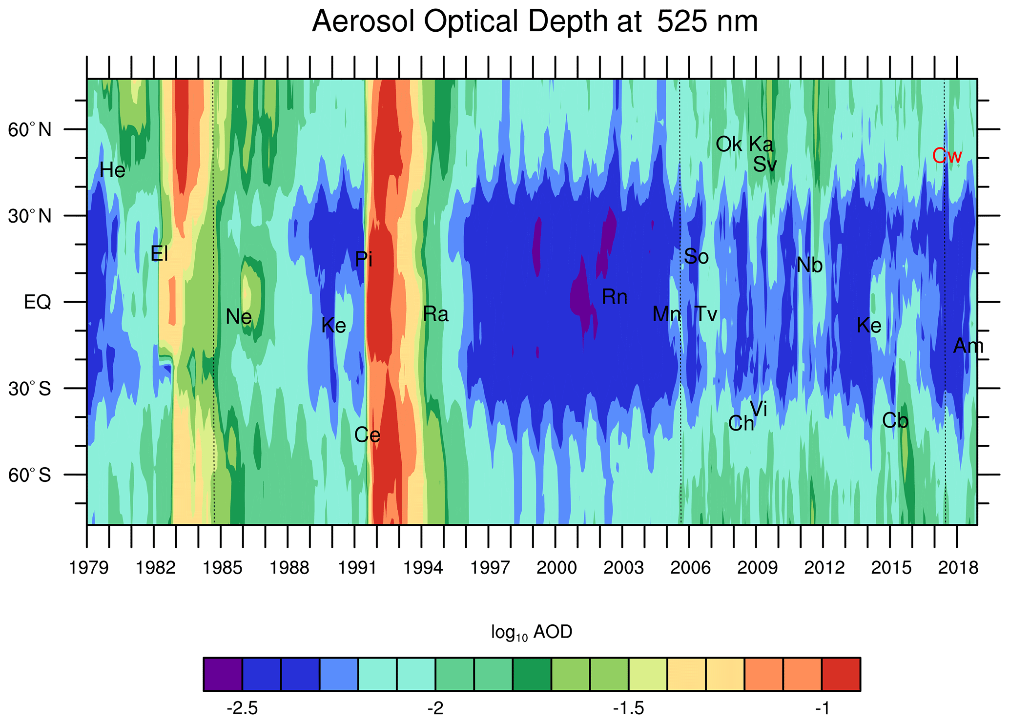
Figure 1Stratospheric aerosol optical depth at 525 nm from GloSSAC v2.0 (Kovilakam et al., 2020). Volcanic and similar events are denoted using the abbreviations given in Table 1. Dotted vertical lines indicate (from left to right) the start of the SAGE II mission in 1984, the end of the SAGE II mission in 2005, and the start of the SAGE III mission in 2017.
Space-based measurements of stratospheric aerosol have been made on a nearly global basis since the Stratospheric Aerosol and Gas Experiment (SAGE; aboard the Applications Explorer Mission 2 platform) operated from 1979 through 1981 (Chu and McCormick, 1979). The SAGE II mission (https://doi.org/10.5067/ERBS/SAGEII/SOLAR_BINARY_L2-V7.0) spanned the recovery of stratospheric aerosol levels from two large-magnitude volcanic eruptions: the eruption of El Chichón in 1982 and the 1991 eruption of Mt. Pinatubo (Thomason et al., 2018). Here, we define large-magnitude eruptions as those with a volcanic explosivity index (VEI; Newhall and Self, 1982) of 6 or more, and small- to moderate-magnitude eruptions as those with a VEI of 3, 4, or 5, whereby we only consider those eruptions that had a measurable impact on the stratospheric aerosol load in the period from 1979 to 2019 (see Table 1). The Mt. Pinatubo eruption was the largest stratospheric event since at least Krakatau in 1883 (Stothers, 1996). In the SAGE II record, the Mt. Pinatubo event remains clearly detectable until the late 1990s; thus, it has an impact on nearly half of the 21-year data set. In the 7 years of SAGE II observations prior to Mt. Pinatubo, stratospheric aerosol levels consistently decrease following the 1982 El Chichón eruption (Thomason et al., 1997a). As a result, nearly 75 % of the SAGE II record is dominated by the recovery from two large-magnitude volcanic events. This can be clearly seen in Fig. 1 where the long-term variation in the stratospheric aerosol optical depth from the Global Space-based Stratospheric Aerosol Climatology (GloSSAC), a global multi-instrument climatology of aerosol optical properties, is shown for 1979 through 2018 (Kovilakam et al., 2020). As a result, due to the timing of the SAGE II mission, much of what is inferred as the “normal” properties of stratospheric aerosol inferred from SAGE II observations is skewed toward these large events rather than a handful of small to moderate events that occur throughout the period of interest.
Table 1Volcanic eruptions and smoke events that significantly impact stratospheric aerosol levels in Version 2.0 of the GloSSAC data set (Kovilakam et al., 2020); these events are denoted in Fig. 1 using the abbreviations in parentheses following their names.
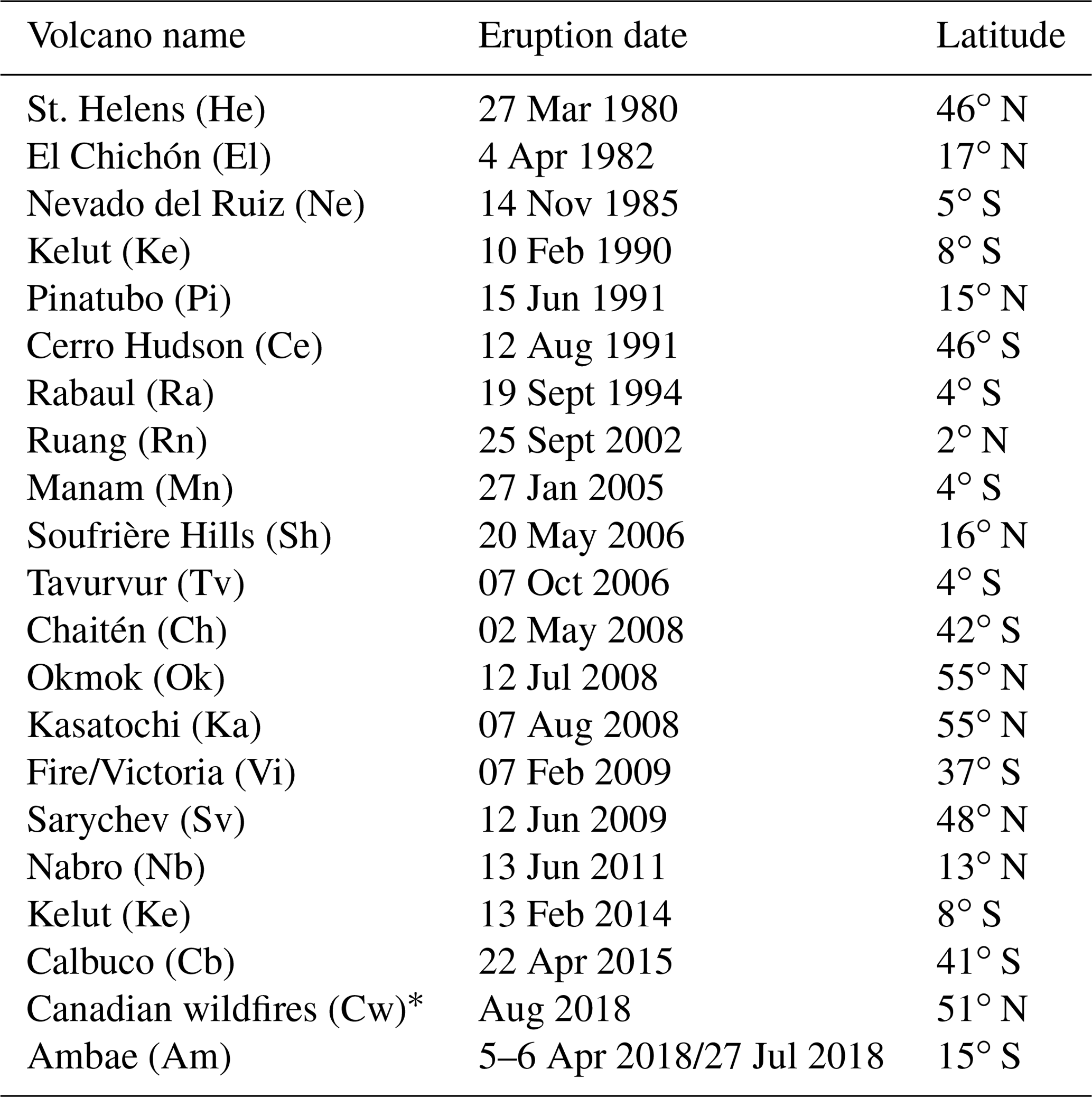
* Canadian wildfires (Cw) occurred in August 2017 and created pyrocumulonimbus (PyroCb) that injected smoke into the stratosphere (Peterson et al., 2018). This event is also marked in Fig. 1.
As shown in Fig. 1, starting with the January 2005 eruption of Manam, which is near the end of the SAGE II record (October 1984 through August 2005), there are regular injections of aerosol and its precursors following volcanic eruptions. While none of these events approached the magnitude of Mt. Pinatubo or El Chichón, they were able to subtly modulate climate and are of general scientific interest (Solomon et al., 2011; Ridley et al., 2014; Schmidt et al., 2018). From the end of the SAGE II mission in August 2005 until the start of the SAGE III/ISS mission in June 2017, space-based missions consist of measurements used in GloSSAC from instruments such as OSIRIS and CALIOP (Rieger et al., 2019; Kar et al., 2019) and data from other instruments including the Scanning Imaging Absorption Spectrometer for Atmospheric Cartography (SCIAMACHY; von Savigny, 2015), the Michelson Interferometer for Passive Atmospheric Sounding (MIPAS; Griessbach et al., 2016), the Ozone Mapping and Profiler Suite Limb Profiler (OMPS LP; Loughman et al., 2018), and Global Ozone Monitoring by Occultation of Stars (GOMOS; Bingen et al., 2017). Since the start of the ongoing SAGE III/ISS mission in June 2017 (https://doi.org/10.5067/ISS/SAGEIII/SOLAR_HDF4_L2-V5.1, last access: 10 February 2020), several additional small to moderate volcanic events have been observed including two eruptions by Ambae (April and July 2018; Kloss et al., 2020b), an eruption by Raikoke (June 2019; Muser et al., 2020), and an eruption by Ulawun (June/August 2019). In addition, there are at least two pyrocumulus (also known as flammagenitus) events, specifically the Canadian forest fire event of August 2017 (Kloss et al., 2019; Bourassa et al., 2019) and the Australian bush fires of December 2019 and January 2020 (Khaykin et al., 2020). These nonvolcanic events are interesting but are not the focus of this paper. After 2005, the frequency of small volcanic and smoke events is substantially higher than observed during the SAGE II mission, and there is a significant qualitative difference in the stratospheric aerosol variability in between the two periods. After the end of the SAGE II mission in 2005 and until the start of the SAGE III mission, the long-term stratospheric record is less robust, which is partly due to the limited global multiwavelength measurements of aerosol extinction coefficient.
It should be clear from the outset that the solar occultation measurement strategy is, in general, not conducive to process studies and understanding the distribution of aerosol following highly localized events like volcanic eruptions. Following these sorts of events, we observe that SAGE observations have a high zonal variance in the data compared with more benign periods where the zonal variance is often not much larger than the measurement uncertainty, particularly in the tropics (Thomason et al., 2010). The events we discuss below are not sampled in a temporally uniform way, and the time between an eruption and the first SAGE II observations at the relevant latitudes varies from a few days to more than a month. This is an outcome of the sparse spatial sampling characteristic of solar occultation, with latitudinal coverage dictated by orbital and seasonal considerations; moreover, a given latitude is measured at best once or twice per month. In addition, with 15 profiles per day with 24∘ of longitude spacing, the sampling is sparse with respect to longitude even when latitudes of interest are available. Furthermore, aerosol properties in a single profile at a single altitude are the average of multiple samples along different line-of-sight paths through the atmosphere such that the spatial extent of a measurement at an altitude extends over hundreds if not thousands of square kilometers (Thomason et al., 2003). This large measurement volume increases the possibility that only part of a SAGE II observation's measurement volume will actually consist of a mix of volcanically derived material and unperturbed stratosphere. As a result, the interpretation of an extinction measurement pair must be carried out in a similar fashion to SAGE observations of water clouds, which are better interpreted as a mixture of aerosol and cloud extinction coefficients rather than purely “cloud” extinction coefficients (Thomason and Vernier, 2013). With these limitations, the ability to characterize the attributes of the early plume is restricted.
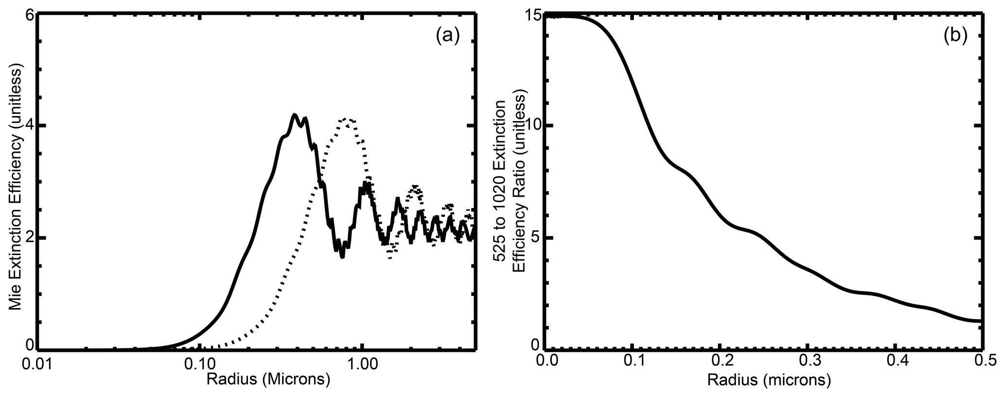
Figure 2(a) Mie extinction efficiency for sulfuric acid droplets at stratospheric temperatures at 525 (solid) and 1020 nm (dashed). (b) The ratio of extinction coefficient at 525 to 1020 nm for single particles as a function of radius for sulfuric acid aerosol at stratospheric temperatures.
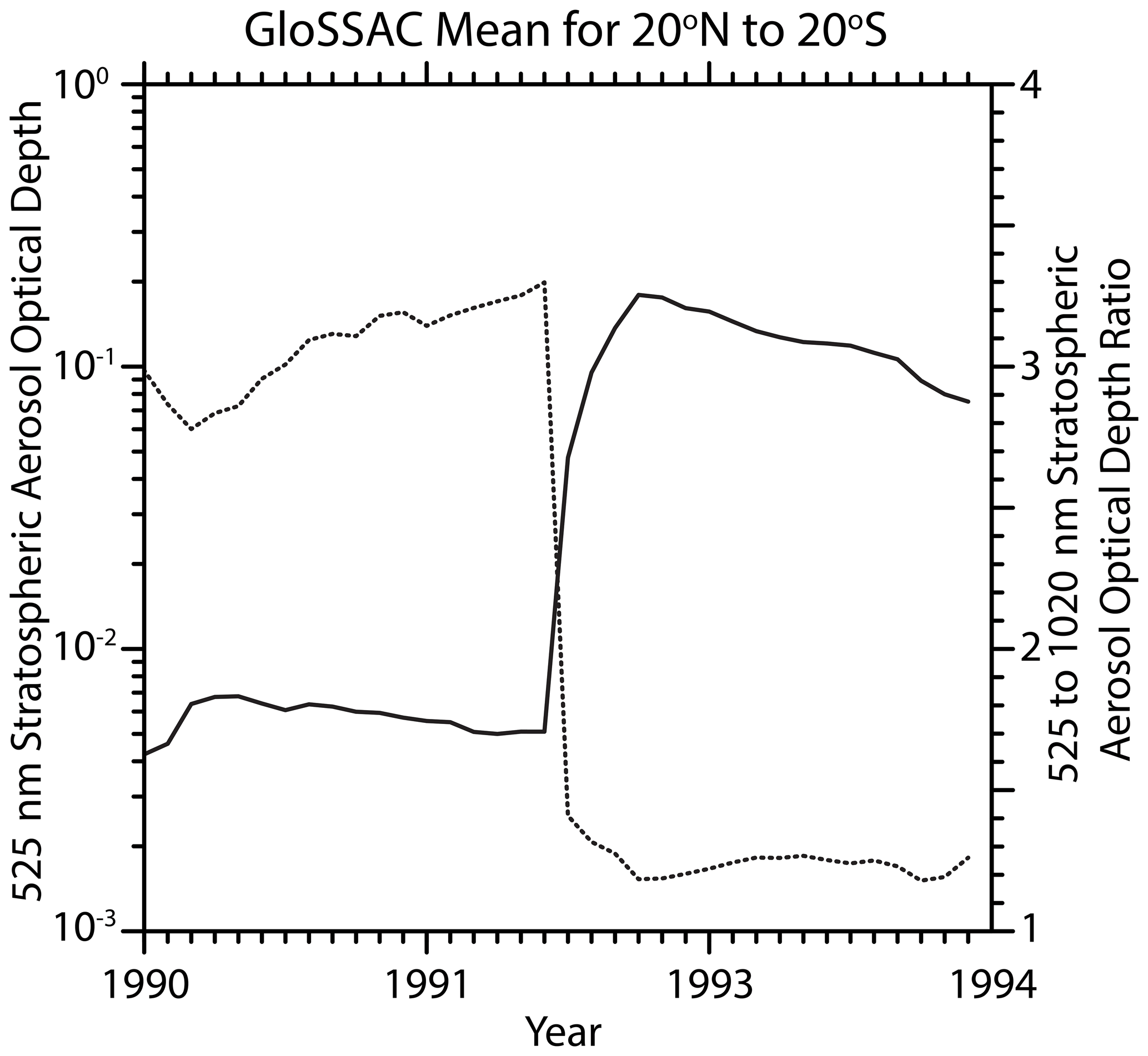
Figure 3The GloSSAC v2.0 depiction of the 525 nm aerosol optical depth (solid) and the 525 to 1020 nm stratospheric aerosol optical depth ratio (dotted) for 1990 through the end of 1993, encompassing the Kelut eruption in early 1990 and the Mt. Pinatubo eruption in mid-1991.
The SAGE instruments use solar occultation to measure aerosol extinction coefficient at multiple wavelengths from the ultraviolet to the near infrared. These measurements are of high accuracy and precision across a broad range of extinction levels, have a vertical resolution of ∼ 1 km, and are reported in 0.5 km increments from 0.5 to 40.0 km (Damadeo et al., 2013). The multiwavelength aerosol extinction coefficient measurements provide limited information regarding the details of the aerosol size distribution (Thomason et al., 2008; Von Savigny and Hofmann, 2020), although many efforts at deriving the aerosol size distribution have been proposed (Yue and Deepak, 1983; Wang et al., 1996; Bingen et al., 2004; Malinina et al., 2018; Bauman et al., 2003; Anderson et al., 2000). The primary measure of particle size for SAGE II comes from the ratio of the aerosol extinction coefficient measurements at 525 and 1020 nm. Figure 2a shows the Mie aerosol extinction coefficient as a function of particle radius at 525 and 1020 nm for sulfuric acid aerosol at stratospheric temperatures (based on Bohren and Huffman, 1998), and their ratio is shown in Fig. 2b . While incorporating a realistic size distribution would complicate the picture, the ratio relationship shows approximately how the inferred aerosol size changes with the extinction coefficient ratio. Over the lifetime of the SAGE II mission, in the stratospheric aerosol layer, this ratio varies from around 5 (∼ 0.2 µm) to values of around 1, where the ability to discriminate aerosol is reduced to noting that the particles are “large” with extinction dominated by aerosol larger than ∼ 0.5 µm. As shown in Fig. 3, the mean GloSSAC v2.0 525 nm stratospheric aerosol optical depth between 20∘ S and 20∘ N, whose construction is discussed in detail in Kovilakam et al. (2020), increased by a factor of about 40 between June and July 1991. At the same time, the 525 to 1020 nm optical depth ratio changed from around 3.3 to a ratio of about 1.2. With low volcanic activity in this period, the relaxation of stratospheric aerosol loading toward background levels remains obvious in the tropics into the late 1990s. The Mt. Pinatubo event can lead to the perception that the “normal” process is that volcanic input into the stratosphere generally increases the aerosol extinction coefficient and decreases the aerosol extinction coefficient ratio (suggesting an increase in the size of particles that dominate aerosol extinction). However, we will demonstrate below that the impact of volcanic events on the stratospheric aerosol extinction coefficient ratio is strongly modulated by the magnitude of the eruption and, to a lesser extent, the stratospheric aerosol loading prior to the eruption. We will also show that the data suggest that sulfur-rich but relatively ash-poor eruptions show a consistent, predictable behavior that lends itself as a test for interactive aerosol schemes used in global climate models. We also observe that the presence of large aerosol, probably ash, following a few eruptions significantly modulates these results.
Table 2Volcanic events observable in the SAGE II (1984–2005) and SAGE III/ISS (2017–present) records including the total number of observations used in the analysis.
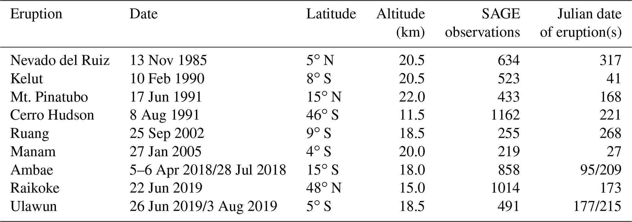
Herein, we examine the impact of 11 eruptions by 9 volcanoes (see Table 2) that affected the stratosphere for which there are SAGE II or SAGE III/ISS measurements available. These begin with the November 1985 eruption of Nevado del Ruiz (Colombia) and continue to the second eruption of Ulawun (Papua New Guinea) in August 2019. Two volcanoes have two eruptions in this record: Ambae in April and July 2017 and Ulawun in June and August 2019. Due to the nature of SAGE III sampling, the Ulawun events cannot be distinguished well and are treated as a single event. Overall, the eruptions increase aerosol extinction coefficient between 10−4 and 10−2 km−1 relative to pre-eruption levels, with a similar relative increase of 2 orders of magnitude compared with the levels observed prior to the eruptions. From observations in the latitude region near the location of each eruption and extending from just prior to each eruption to several months following the eruption, we infer the impact of these eruptions by noting the perturbation on the stratospheric aerosol extinction at both 525 and 1020 nm when the extinction coefficient at 1020 nm is at a maximum. The ratio of these perturbations provides a rough assessment of the impact of the eruptions on the size of particles dominating aerosol extinction. We analyze data from SAGE II and SAGE III/ISS in identical ways except for one detail. The current version of SAGE III data (5.1) has a defect in which aerosol extinction at 521 nm is biased low below about 20 km due to an error in the O4 absorption cross section used in processing this version. The O4 error has a subtle, positive impact on the ozone retrieval below 20 km where there is significant overlap in the spectral regions used to retrieve ozone and where O4 absorbs. The small error in ozone has a larger impact on aerosol where ozone absorbs strongly (521, 602, and 676 nm), but other aerosol measurement wavelengths are unaffected. Therefore, we have replaced the 521 nm data product with an interpolation between 448 and 756 nm that employs a simple Ångström coefficient scheme. The 448 and 756 nm aerosol extinction coefficients do not manifest the bias, whereas 602 and 676 nm measurements have biases similar to those at 521 nm. The interpolation is possible as stratospheric aerosol extinction coefficient is always observed to be smoothly varying with wavelength and approximately linear in log–log space. The presence of the 521 nm bias is inferred using this methodology, and this approach was used in the validation paper for SAGE III/Meteor 3M aerosol data (Thomason et al., 2010). The differences between the inferred 521 nm extinction coefficients and the reported values in the lower stratosphere (tropopause to 20 km) average about 6 % and are usually less than 10 %. Above 20 km the differences are usually on the order of 1 % to 2 % with the estimate usually less than the observation; this is probably a reflection of the limitation of the accuracy of the interpolation and is consistent with past uses of the same approach (Thomason et al., 2010). In any case, the same arguments regarding the effects of small to moderate volcanic eruptions on aerosol extinction coefficient as a function of wavelength described below can be made whether the 448 or 521 nm aerosol extinction coefficient is used in the SAGE III analysis. We interpolate the 521 nm values solely for comparison with SAGE II data, and this process has minimal impact on the conclusion drawn below.
For each event, we collect all SAGE II/III aerosol extinction coefficient data at 525 and 1020 nm between 10 and 25 km where the profiles occur within 10∘ latitude of the eruption for a period starting 3 months prior to the eruption until 6 months following it. Depending on the latitude, as recorded in Table 2, and season, the volume and frequency of observations can vary significantly. Figure 4a shows all of the data for Nevado del Ruiz in this temporal window at the altitude of the maximum increase in aerosol extinction coefficient – in this case 20.5 km. The Nevado del Ruiz eruption occurred on 13 November 1985 (Julian day 317), and the immediate enhancement of aerosol extinction coefficient is clear: aerosol extinction coefficient increases by about an order of magnitude from about 0.0007 km−1 to values approaching 0.01 km−1. As shown in Fig. 4b, the aerosol extinction coefficient ratio increases from about 2.2 prior to the eruption to a broad range of values from 2 to 3.5 immediately following the eruption (∼ Day 380 or January 1986); this is the inverse of what was observed following the Mt. Pinatubo eruption, as shown in Fig. 3. The Nevado del Ruiz extinction ratio becomes much more consistent in the subsequent samples of this region of the stratosphere and falls from roughly 2.8 to 2.4 at the end of the analysis period (∼ Day 560 or July 1986). The early spread in extinction coefficient and in the extinction coefficient ratio is primarily due to inhomogeneity in the volcanic aerosol within the analysis area (Sellitto et al., 2020). This is suggested by Fig. 5 in which the extinction coefficient ratio is plotted versus extinction coefficient for this data set. Almost without exception, the enhancement in aerosol extinction coefficient is associated with larger extinction coefficient ratio values. The distinction between volcanically perturbed observations and the unperturbed periods prior to the eruption is clearly recognizable. A handful of points show very high aerosol extinction coefficients but extinction coefficient ratios close to and occasionally less than those observed prior to the eruption (< 2.3 or so). For these observations, some large particles (possibly ash) are evidently present; however, as SAGE-like observations contain little or no information about composition, their composition cannot be inferred unambiguously. In any case, these points are rare and are only observed in the first month following the eruption, which is possibly due to the removal of large particles by sedimentation. Generally, we find that the low-latitude eruptions like Nevado del Ruiz exhibit less zonal variability in aerosol extinction coefficient than mid- and high-latitude events. For instance, SAGE III/ISS observations of the Canadian pyrocumulus event in August 2017 (Bourassa et al., 2019) varied with respect to extinction coefficient at some latitudes from a pre-event extinction of 10−4 km−1 to values that exceeded 10−2 km−1 as late as the end of October 2017. In this regard, low-latitude events are a more straightforward evaluation than high-variability, higher-latitude events.
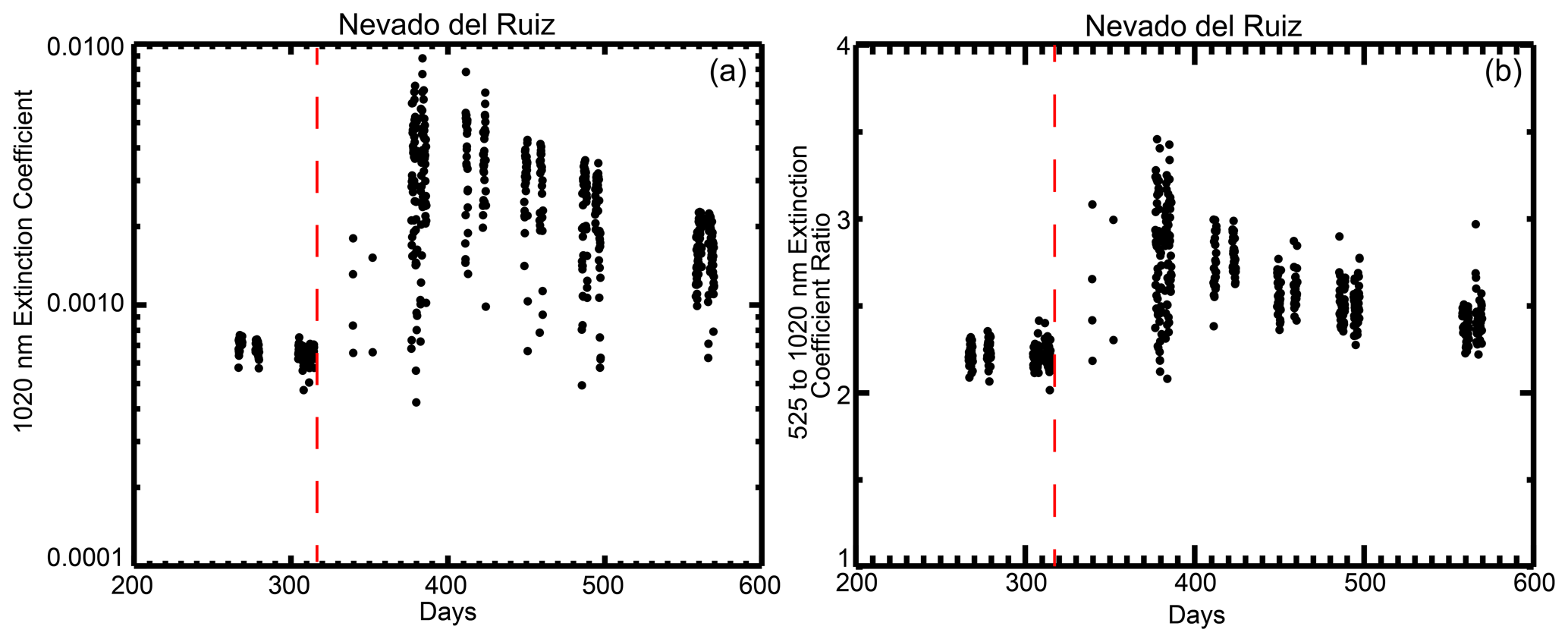
Figure 4The time series of the SAGE II 1020 nm aerosol extinction coefficient (in km−1) (a) and the 525 to 1020 nm aerosol extinction coefficient ratio (b) at 20.5 km between 10∘ S and 10∘ N in days from 1 January 1985 (Day 1); thus, the first day is 19 July 1985, the eruption occurs on Day 317 (13 November 1985), and the plot ends on 23 August 1986. The date of the eruption is denoted by a vertical dashed red line.

Figure 5The same data as shown in Fig. 4a and b except now plotted as the 1020 nm aerosol extinction coefficient (in km−1) versus the extinction coefficient ratio. The extinction coefficient ratio is a rough estimate of the size of aerosol particles that dominate extinction. Values near 1 suggest a particle radius greater than ∼ 0.4 m with increasing values indicating smaller particles. Values for observations prior to the eruption are red. All data are for 20.5 km.
Given the geometry of the solar occultation measurements, SAGE II and III sample a latitude band episodically, revisiting a latitude every few weeks to months and making observations in a latitude band for 1 to several days. This sampling pattern is clear in Fig. 4a and b. We defer to this pattern and average the extinction values at both 525 and 1020 nm into these irregularly spaced temporal duration bins. We required a minimum of six profiles to be available in the temporal bin for the bin to be included in further analysis. This eliminates a few periods, such as the few points around Julian day 340 and around Julian day 350, as seen in Fig. 4a. Within each bin, we select the maximum values of the extinction coefficient at 1020 nm in each profile within a 4 km vertical window (nine observations) that extends from 1 km below to 3 km above the broadly observed maximum in the extinction profiles (20.5 km in this case); this vertical window is chosen because we try to capture the behavior of the most intense part of the volcanic layer, including the tendency for the layer to increase in altitude during the months following the eruption. The 4 km window is primarily a way to find the altitude (and the associated extinction coefficients) of the volcanic layer in each profile, as it can vary from profile to profile, within a temporal bin, and over the months following the eruption. For events in this analysis, there is a 0.5 to 2 km rise in the altitude of the peak aerosol extinction coefficient during the analysis period following the eruption, which is mostly due to dynamical processes (Vernier et al., 2011). The averaging produces a simplified characterization of the effects of the eruption, as shown in Fig. 6. In this figure, we see that the change in aerosol extinction coefficient and extinction coefficient ratio are well correlated, with both reaching a maximum near Julian day 380 (as sampled by SAGE II). One difference is that while both parameters begin to relax back toward pre-eruption levels, extinction coefficient does so faster than the extinction coefficient ratio. As the scale for the extinction coefficient ratio does not extend to zero, the difference in the recovery rates is even more significant. Figure 7 shows the same plots for the remaining nine eruptions. They can be crudely sorted into two categories. While all show relatively rapid increases in the aerosol extinction coefficient at 1020 nm with the maximum values occurring with the first or second observation by SAGE II/III, one category of eruption is similar to the Nevado del Ruiz eruption, showing rapid increases in the aerosol extinction ratio following the eruption. These tend to be among the smaller eruptions and include Cerro Hudson in 1991 (Fig. 7c), Manam in 2005 (Fig. 7e), Ambae twice in 2018 (Fig. 7f), and Ulawun twice in 2019 (Fig. 7g). In the case of the second Ambae eruption, there is a small increase in the observed aerosol extinction coefficient ratio following the eruption, and it remains large (∼ 4.8) compared with the value prior to the first Ambae eruption (∼ 3.2). A second category of volcanic events shows the opposite behavior, with a decrease in the extinction ratio following an event; such events include Kelut in 1990 (Fig. 7a), Mt. Pinatubo in 1991 (Fig. 7b), Ruang in 2002 (Fig. 7d), and Raikoke in 2018 (Fig. 7g). We will now discuss some individual events.
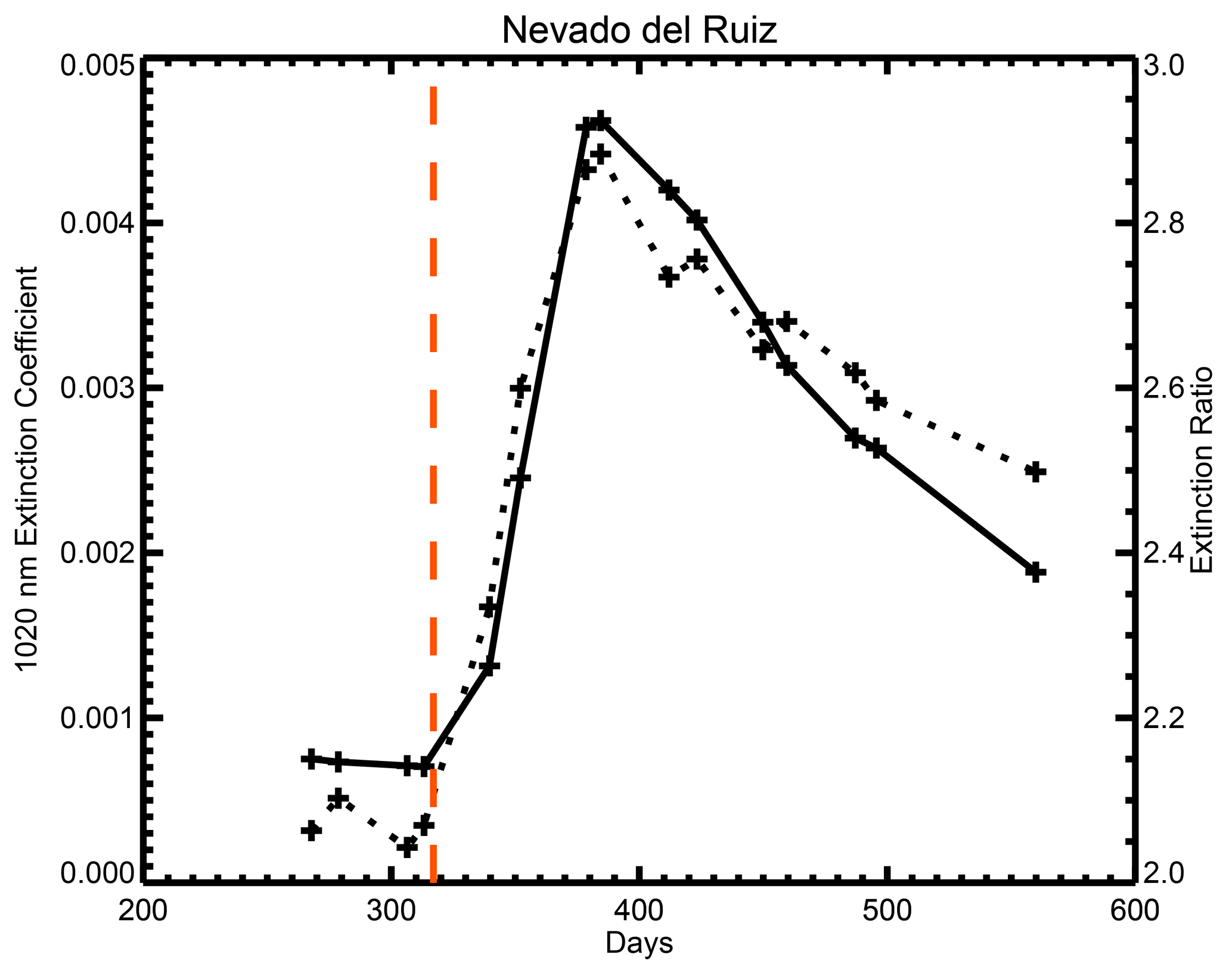
Figure 6Same data as shown in Fig. 4 except averaged in temporal data clusters. In this figure, extinction coefficient is the solid line and the extinction coefficient ratio is the dotted line. The date of the eruption is denoted by the vertical red dashed line.
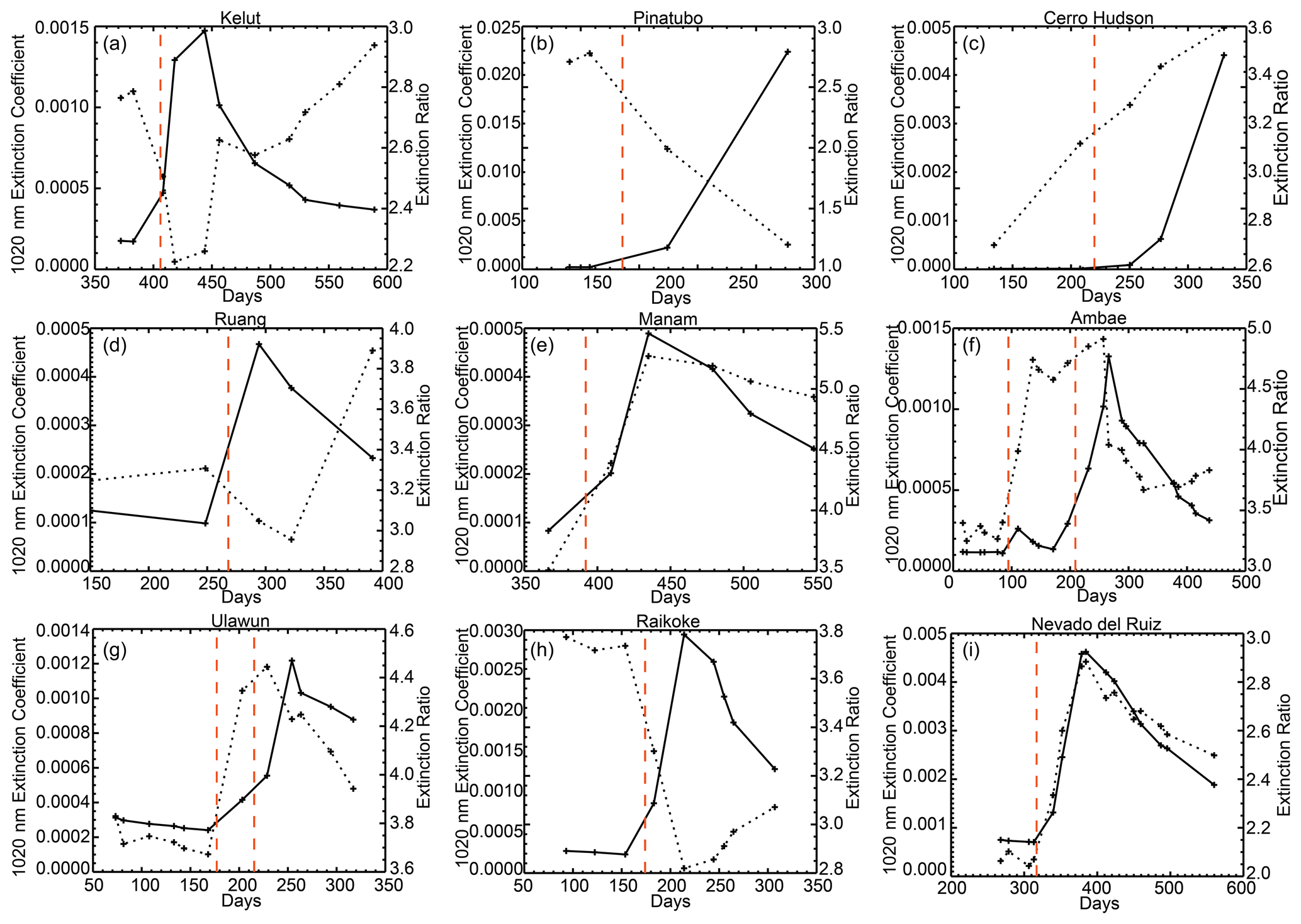
Figure 7Similar analysis as that shown in Fig. 6 except for Kelut in 1990 (a); Mt. Pinatubo (b) and Cerro Hudson (c) in 1991; Ruang in 2002 (d); Manam in 2005 (e); Ambae in 2018 (f); and Ulawun (g) and Raikoke (h) in 2019. In each frame, extinction coefficient is the solid line and the extinction coefficient ratio is the dotted line. The dates of the eruptions are denoted by the vertical red dashed lines. The plot for the Nevado del Ruiz eruption shown in Fig. 6 is repeated here in panel (i) for comparison. Days refer to the number of days since the start of year in which the analysis begins for an individual eruption. For panels (a) to (i) these years are 1989, 1991, 1991, 2002, 2004, 2018, 2019, and 2019, respectively.
Figure 8a shows the before and after state of the main aerosol layer for these 10 eruptions. Here, “before” values are defined as the first data point in the series shown in Fig. 7, and “after” values are defined as the point where the 1020 nm aerosol extinction coefficient reaches a maximum. As one could infer from Fig. 7, we see two types of events – those with positive slopes (larger extinction ∕ larger extinction ratio) and those with negative slopes (larger extinction ∕ smaller extinction ratio) – with some suggestion of a change in slope from strongly positive to negative with increasing aerosol extinction coefficient perturbation. To isolate this change, we define an aerosol extinction coefficient perturbation as
which is computed for 1020 and 525 nm, where the 1020 nm aerosol extinction coefficient is a maximum. It should be noted that the maximum extinction coefficient at 525 nm does not necessarily occur at the same altitude or time as the maximum in the 1020 nm extinction coefficient. There is some variability in the timing of the before data used in this analysis; however, within these data sets, we observe that aerosol extinction coefficient levels at a given altitude and latitude slowly vary with time independent of recent volcanic activity due to the recovery from past volcanic activity and seasonal processes. For the events discussed here, due to the timing of the events, these changes are very small compared with the volcanic events in our study and, in terms of the calculation of perturbation values, the exact background level only has a secondary effect on the calculated values. As a result, the timing of the before samples does not materially affect these results. We define an aerosol extinction coefficient perturbation ratio (or more simply perturbation ratio) as

Figure 8The “before” (left-hand point) to peak 1020 nm aerosol extinction coefficient (right-hand point) for the 10 eruptions considered in this study is shown in panel (a), and the differences between them (perturbations) are shown in panel (b).
Figure 8b shows the relationship between the perturbation parameters. The perturbation ratio for eight of these events is well sorted by the magnitude of the extinction coefficient perturbation from the smallest extinction coefficient perturbation event (Manam) to the largest (Mt. Pinatubo). Based on Fig. 2b, we would expect that the relationship would asymptote to about one for large events close to or larger than Mt. Pinatubo, reflecting the presence of very large radius aerosol (>0.4 µm); thus, some sort of curvature seems reasonable. It should be noted that SAGE II did not observe the entirety of the Mt. Pinatubo plume due to its extreme opacity. However, the available observations uniformly show very high extinction (>10−2 km−1) and a low extinction ratio (∼ 1) with all observations. Therefore, while the detailed location of the Mt. Pinatubo data in plots 7 and 8 is not exact, the general location, particularly in Fig. 8b, is representative of this event. While the perturbation ratio approach effectively treats the aerosol as an add-on to the before aerosol extinction, we do not suggest that volcanic aerosol does not interact with the pre-existing aerosol. Nonetheless, the observed relationship in Fig. 8b suggests that the values of the perturbation pair (extinction coefficient and perturbation ratio) are insensitive to the initial conditions of the stratospheric aerosol. This relationship suggests a potential route to inferring uncertainty in the OSIRIS and CALIOP data during the SAGE II to SAGE III/ISS gap period by estimating changes in the extinction coefficient slope (or Ångström coefficient) based on perturbations in those instruments' measured quantities. There is uncertainty regarding the details of this analysis, particularly as it relates to the timing of the measurements following the eruption; thus, the apparent linearity of the eight data points should be interpreted cautiously. Nonetheless, it should be possible for ESMs and GCMs with detailed aerosol microphysical models to calculate aerosol extinction coefficient at any wavelength; therefore, this analysis may provide the opportunity for a small to moderate volcanic plume closure experiment.
Despite the close timing of the two Ambae eruptions in 2018 (April and July), the eruptions are clearly distinguishable in the SAGE III/ISS data shown in Fig. 7f, with the later eruption being many times more intense than the earlier one (Kloss et al., 2020b). Individually, the Ambae (Vanuatu) eruptions in 2018 are similar to the Nevado del Ruiz eruption that is discussed in detail above, as both show an increase in extinction coefficient and extinction coefficient ratio relative to the values seen in early 2018 (which is characteristic of most small to moderate eruptions). However, the extinction coefficient ratio decreases following the second eruption, suggesting that the second eruption may be an outlier to the generally observed behavior. To calculate the perturbations for these two events, we use data from prior to the first eruption as the before values for both, although the results for the second eruption are insensitive to the perturbation caused by the earlier eruption. The initial Ambae eruption increased the extinction coefficient ratio from 3.2 to 4.7 with an increase of 1020 nm extinction from approximately 10−4 to about km−1. The second eruption initially increases the extinction coefficient ratio from 4.5 just prior to the eruption to 4.9 with the earliest observations shortly after the eruption; this value subsequently decreases to 4.1 when aerosol extinction coefficient is at a maximum. Aerosol extinction coefficient increases from to km−1 or by about a factor of 6 (Fig. 7f). With these values, and despite appearances, both eruptions fit well with the majority of the other events (Fig. 8b). In this case, the eruptions occur at slightly different altitudes, so the apparent rise in the aerosol layer from the beginning to the end of the period is a little larger than for most events (∼ 2 km). In this case, particularly for the second eruption, the extinction change is so large that the impact of the pre-eruption aerosol values is negligible. Another interesting feature is that the largest ratios after the eruption do not necessarily coincide with the largest extinction. Figure 9 shows the extinction latitude–altitude cross sections for September 2018 for 521 nm (Fig. 9a) and 1020 nm (Fig. 9b) as well as their ratio (Fig. 9c). It is clear here that the maximum in the extinction ratio lies below the main peak in the extinction coefficient in the tropics and notably stretches to higher southern latitudes; however, the maximum extinction ratio value actually occurs near 30∘ S despite more inhomogeneous conditions at this latitude than in the tropics. This is not an obvious outcome, but it is consistent with the general observation that the largest perturbations in the extinction ratio occur with smaller extinction coefficient perturbations, as shown in Fig. 8b. It also shows the importance of keeping in mind that the relationship between extinction coefficient perturbation and the overall extinction ratio in Fig. 8b is for the densest part of the volcanic plume and not for all parts of the volcanic cloud. The fact that the dependence of the aerosol extinction coefficient perturbation ratio on extinction coefficient perturbation occurs within a particular eruption as well as among different eruptions (for the peak values shown in Fig. 8) implies that a consistent physical process is at work.
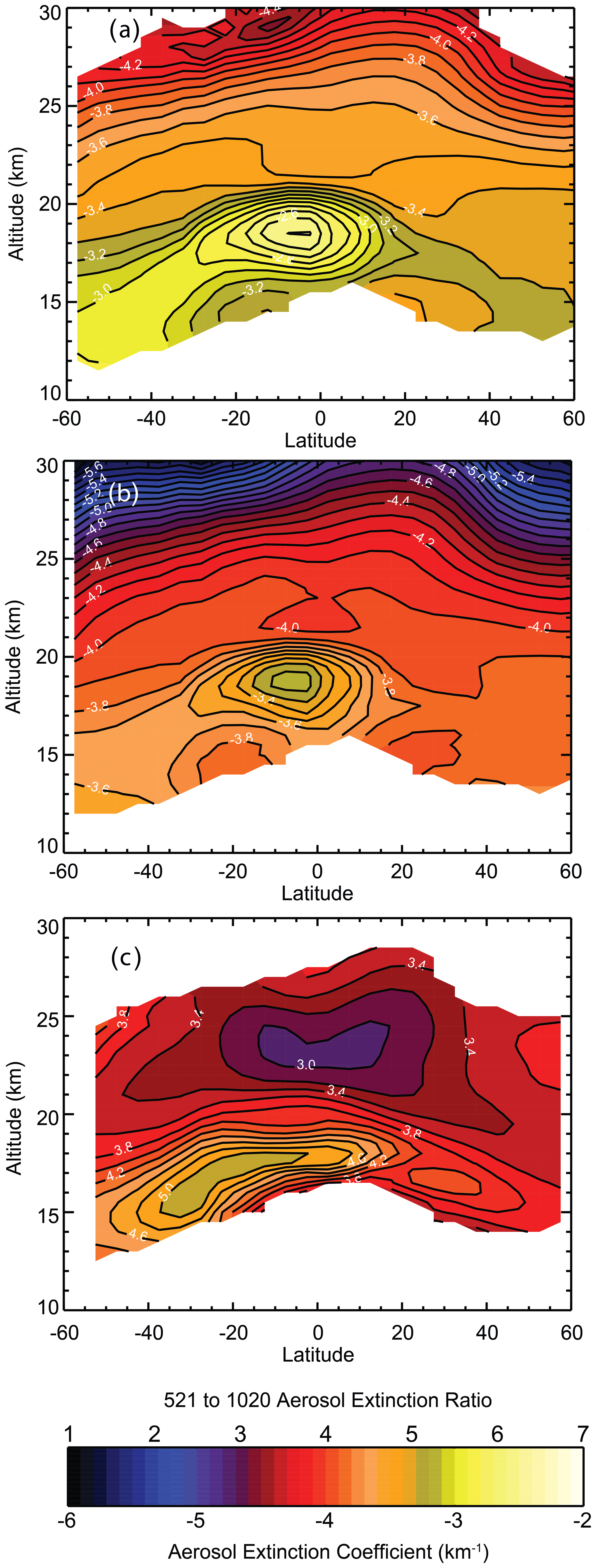
Figure 9The mean SAGE III/ISS 525 (a) and 1020 nm (b) aerosol extinction coefficient and the 525 to 1020 nm aerosol extinction coefficient ratio (c) as a function of latitude and altitude from September 2019, shortly after the second 2019 eruption of Ambae (July 2019; 15∘ S).
There are two events lying a considerable distance from the main curve in Fig. 8b: Ruang and the 1990 eruption of Kelut. For Kelut, the first observations of the plume take place about 10 d after the eruption. This is where the extinction ratio is the lowest (Fig. 7a); it increases from 2.2 to 2.6 in the following few weeks and then to 2.9 at the end of the observation period. Ruang shows some similar features, with the low perturbation ratio (2.9) occurring shortly after the eruption followed by a recovery toward larger values in the weeks that follow (3.9). The Kelut scatterplot (Fig. 10) shows that while the scatter of extinction coefficient and ratio are compact for most of this period, there are some observations of higher extinction and ratios approaching one that occur in the earliest observation period, suggesting the immediate presence of large aerosol (>0.5 µm). While the data do not inherently provide certainty, it is possible that an extinction-dominating presence of ash particles rather than sulfuric acid particles in the main aerosol layer immediately after the eruption may push the perturbation location below the rough curve suggested by most of the events. Similar data from Ruang are less illuminating due to a much smaller sample in the 50 % duty cycle period of SAGE II data (after the end of 2000), and it is not possible to infer a cause for their anomalous position in Fig. 8b. Both eruptions show increased aerosol extinction coefficient ratios away from the main aerosol peak, suggesting, at least in part, behavior more consistent with most eruptions.
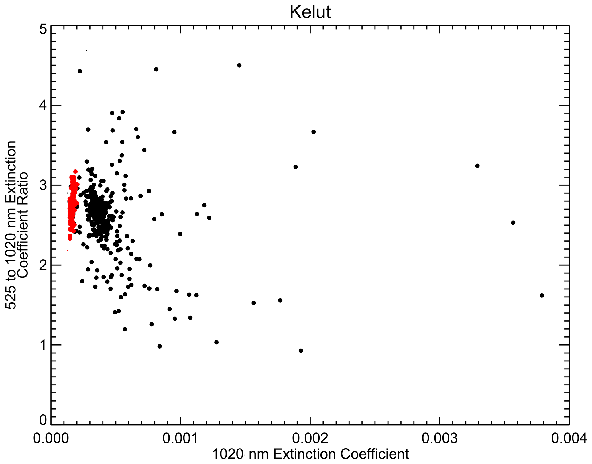
Figure 10The SAGE II 525 to 1020 nm aerosol extinction coefficient ratio plotted versus the 1020 nm aerosol extinction coefficient (in km−1) during the Kelut event from December 1989 through August 1990 plotted at 20.5 km between 20∘ S and the Equator. Measurements occurring before the eruption are colored red.
Another interesting feature are differences between the Nevado del Ruiz, Cerro Hudson, and Raikoke eruptions which cause very similar extinction coefficient perturbations but different perturbation extinction ratios. The position of Nevado del Ruiz in Fig. 8b is consistent with the overall perturbation relationship. Raikoke lies on the same side as the Kelut and Ruang eruptions but, unlike Kelut, there is little evidence of a mix of increased extinction coefficient observations with small and large extinction ratios (large particles inferred to be ash but possibly other compositions) at the peak extinction level, as the data essentially uniformly show small extinction coefficient ratios following the mean relationship in Fig. 7g. As Raikoke is one of only two midlatitude eruptions in the data set, it is possible that latitude plays a role in the perturbation relationship. However, Cerro Hudson lies closer to Nevado del Ruiz's position and is a similar event to Raikoke: it occurs at a similar latitude (although opposite hemisphere) and in a similar season as well as at a similar pre-eruption aerosol extinction coefficient level. It is possible that atmospheric conditions or some detail of eruptions can have a modulating impact on how events manifest themselves with respect to extinction coefficient and ratio but not be easily detectable from the data alone. For instance, for Raikoke, we cannot exclude the possibility of the presence of small amounts of ash embedded in the main aerosol layer with the sulfuric acid aerosol influencing extinction coefficient and ratio. The presence of ash following the Raikoke eruption has been inferred above 15 km and perhaps as high as 20 km (Muser et al., 2020; Kloss et al., 2020a). In this case, it is possible that the ash is coated with sulfuric acid and that these particles may freeze. It is also possible that pyrocumulus events in Alberta, Canada, and Siberia, occurring around the time of the Raikoke eruption (Yu et al., 2019), played a role in the evolution of extinction following this event. Overall, there are substantial opportunities for complex optical properties in this eruption. To some extent, while we are fortunate to have as many events for this analysis as we do, it is still a relatively small sample, and some factors that can impact the extinction coefficient–extinction ratio relationship may not be fully revealed.
Based on the observations discussed above, although without a detailed simulation of the aerosol microphysical processes at play, we speculate that most small to moderate eruptions are initially dominated by small (∼ 1 nm), mostly homogeneously nucleated sulfuric acid particles that are present in very large number densities (Deshler et al., 1992; Boulon et al., 2011; Sahyoun et al., 2019). As shown in Fig. 2a, due to their small size, these particles are initially extremely poor scatterers and, thus, would not impact the SAGE-like extinction measurements. However, as they coagulate into steadily larger particles (possibly also consuming small-sized aerosol present in the pre-existing aerosol layer) and further condensation occurs, they would produce perturbations to the observed aerosol extinction and ratio that reflect their magnitude. This process generally causes an increase in the aerosol extinction coefficient ratio but may produce the opposite effect depending on the properties of the aerosol present prior to the eruption (which is discussed in more detail below). The coagulation process continues producing ever-larger aerosol and smaller particle number densities until coagulation is no longer efficient at the timescales we examine here and with respect to mixing of the material within the stratosphere. Some eruptions, like that of Raikoke in 2019, clearly depart from this conceptual model as we discuss further below. For large-magnitude eruptions, like Mt. Pinatubo, it is possible that volcanic precursor gases and sulfuric acid vapor primarily condense onto existing aerosol and these, as well as very small homogeneously nucleated aerosol particles, rapidly (compared to the measurement frequency of SAGE-like measurements) coagulate to form much larger-sized aerosol than after small-magnitude eruptions; thus, the aerosol extinction coefficient ratio decreases extremely rapidly toward a value of one. This alternative is not consistent with the observations of most small to moderate eruptions shown in Fig. 8, and the conceptual model we describe below is not intended to capture this behavior.

Figure 11The estimated 525 to 1020 nm aerosol extinction ratio and the 1020 nm aerosol extinction coefficient for the second Ambae eruption (a, c) and Nevado del Ruiz (b, c) computed using fixed aerosol volume density perturbations and single-radii particles that yield an extinction coefficient perturbation at 525 nm of 10−4 (solid), 10−3 (dotted), and 10−2 km−1 (dashed) using rough “before” 525 and 1020 nm extinction coefficient values for each eruption.
To demonstrate how the homogeneous nucleation and coagulation process could impact SAGE-like observations, we have used a conceptual model that simulates a volcanic perturbation as single-radii sulfuric acid particles that begin at a 1 nm radius and grow to large particle sizes (500 nm) but hold the total volume of new aerosol material constant. The goal is to show that the large aerosol extinction coefficient perturbation ratios observed following small to moderate eruptions are consistent with the presence of many small particles that grow through coagulation to larger particles with smaller extinction ratios. The model also shows why similar-sized eruptions can appear differently in extinction coefficient measurements depending on the state of stratospheric aerosol prior to the eruption. This is an extremely simple view of how the aerosol size changes after an eruption and cannot capture the details of the microphysical processes going on in the volcanic aerosol layer; nonetheless, we believe that it provides a reasonable interpretation of the observations as well as a starting point for a model for post-volcanic aerosol spectral dependence that could be useful for OSIRIS and similar measurements including a degree of predictability for events not measured by SAGE instruments, such as Sarychev, Kasatochi and Nabro. It may also be useful in comparisons of SAGE-like observations and results from GCMs and ESMs.
For the model, we determine the volume density of aerosol required to produce 1020 nm extinction coefficient perturbations of 10−4, 10−3, and 10−2 km−1 at a single radius of 500 nm. This can be expressed using
and
where δkλ is the extinction coefficient perturbation at wavelength λ (in this case 1020 nm), r is perturbation particle radius (500 nm), n(r) is the inferred perturbation particle number density, Qλ(r) is the Mie extinction efficiency for the wavelength (shown for 525 and 1020 nm in Fig. 2a) and radius considered for sulfuric acid aerosol at stratospheric temperatures, and V is the required volume density of aerosol. The choice of 500 nm for this calculation is somewhat arbitrary, and the use of any value would not affect the conclusions drawn from this study. For an extinction perturbation of 10−2 km−1, the number density is 4.50 cm−3 with a volume density of 2.37 µm3 cm−3. Holding V fixed, we compute the number density and the aerosol extinction coefficient perturbation as a function of radius at 525 and 1020 nm using
and
for a radii, r, from 1 to 500 nm. The ratio of these extinction coefficient perturbations follows the relationship shown in Fig. 2b. Finally, we add before aerosol extinction coefficient values that we previously determined for the Nevado del Ruiz eruption and the July 2018 Ambae eruption and show these relationships in Fig. 11a and c, respectively. Due to their different pre-eruption extinction levels, the extinction ratio plots shown for the two volcanic events are notably different despite having identical extinction coefficient perturbations at 525 and 1020 nm, which were computed using the above relationships. This is consistent with the data shown in Fig. 8a. To some extent, the radius axis in this plot is akin to a time axis, although a particularly nonlinear one. It is likely that the transition across the smallest size particles is extremely rapid (relative to SAGE-like observation timescales at least), and the large end of the timescale may effectively be reached rapidly for large events like Mt. Pinatubo but effectively never for small to moderate eruptions due to the other processes that control coagulation and other aspects of aerosol morphology. Indeed, the first observations of the main Mt. Pinatubo cloud in early July 1991, a few weeks after the eruption, show an extinction coefficient ratio of essentially one. Whether this would have been the case for observations immediately after the eruption is an interesting unknown. In the aftermath of the second Ambae eruption, as shown in Fig. 7f, the aerosol extinction coefficient ratio maximum occurs before the extinction maximum at 1020 nm, and the ratio has in fact decreased by the time the extinction coefficient at 1020 nm is at a maximum. This is reproduced by the model for the “Ambae” eruption where the maximum in the aerosol extinction ratio is observed at significantly smaller radii (Fig. 11a) than the radii for which the 1020 nm aerosol extinction coefficient is at a maximum (Fig. 11b). This behavior is also exhibited in the model for the Nevado del Ruiz eruption, where the aerosol extinction coefficient perturbation ratio (shown in Fig. 11c) does not reach such a high peak; nonetheless, it clearly reaches a maximum at smaller radii than the 1020 nm aerosol extinction coefficient maximum in Fig. 11d.
If the initial growth to 200 nm is rapid at SAGE temporal sampling scales (∼ monthly), the model simulations qualitatively reproduce the increase in the extinction coefficient ratio seen in many of the eruptions analyzed with a step increase in the extinction coefficient ratio followed by a decrease in time. In addition, these results show that, while the extinction coefficient perturbations themselves may be insensitive to the before stratospheric state, the result is not. In fact, scenarios can be easily constructed in which the same eruption, again with minimal interaction with the pre-existing aerosol, results in a different sign in the slope of the change in the extinction coefficient ratio. Obviously, we must exercise caution in interpreting the observations based on the simple model employed here. For instance, as we do not know the timescale of coagulation, significant uncertainty remains in how to interpret Fig. 8b in a temporal sense. Moreover, the aerosol volume density is unlikely to be constant over this time as the conversion of SO2 to H2SO4 has a time constant on the order of 30 d and depends on the magnitude of the eruption. Nonetheless, while not a primary goal of this study, we argue this very simple model suggests that SAGE II/III observations are consistent with volcanic material primarily nucleating homogeneously followed by coagulation, whose timescale depends on the magnitude of the eruption. In the end, however, certainty can only be obtained via closure experiments between observations such as these and GCMs and ESMs with detailed microphysical models.
Herein, we have used SAGE II/III observations to examine the behavior of stratospheric aerosol extinction coefficient in the aftermath of small- to large-magnitude volcanic events with the primary goal of understanding how these events manifest themselves in SAGE-like observations. We have focused on initial plume development at peak extinction levels, not on the long-term development or details of its distribution, as transport and other aerosol processes such as sedimentation have not been considered. At peak extinction levels, under most circumstances, we have found that observations of the impact of volcanic eruptions on stratospheric aerosol, as measured by the SAGE series of instruments, show a crude independence of the characteristics of the pre-existing aerosol and a correlation between the magnitude of the enhancement in aerosol extinction coefficient and its wavelength dependence, as shown in Fig. 8b. While this relationship is insensitive to the pre-existing aerosol level, the pre-existing aerosol can modulate the observed changes in the aerosol extinction coefficient ratio. The analysis is straightforward for tropical eruptions but more challenging for mid- and high-latitude eruptions where transport is generally more complex than in the tropics. Also, it is possible that volcanic events with significant amounts of ash may behave considerably differently from those dominated by the sulfuric acid component.
The perturbation relationship, shown in Fig. 8b, is only based on the measurements themselves and makes no assumptions about the underlying composition or size distribution of the aerosol. In this respect, it is a unique tool to intercompare observations and interactive aerosol models used in GCMs and ESMs. This should be extremely straightforward as extinction coefficients can be calculated from aerosol products already produced by these modules, although care would need to be exercised to reproduce the observations used herein. As the results span a large dynamic range of aerosol extinction coefficient perturbations (> 2 orders of magnitude), the testing range covers a significant range of volcanic events. As the observed relationship is well-behaved, testing is potentially not limited to observed volcanic events but may be applied to hypothetical events or historical events for which space-based observations do not exist.
A longer-term goal is to assess the data quality of data sets consisting of a single-wavelength measurement of aerosol extinction coefficient or similar parameters, particularly when a fixed aerosol size distribution is a part of the retrieval process. This is important as a part of the data quality assessment of these data sets as well as their use in long-term data sets such as GloSSAC. In this regard, the results are mixed. It is clear from Fig. 8b that the wavelength dependence of a predominant sulfuric acid volcanic event can be estimated from the relationship shown therein. As a fixed particle size distribution is used in the OSIRIS retrieval process, a fixed wavelength dependence is effectively intrinsic to the OSIRIS aerosol extinction coefficient retrieval process. The use of these results in OSIRIS retrievals is an ongoing study which we hope will result in positive improvements in the OSIRIS aerosol data products in the future. In the short-term, we believe that we may be able to use these results in spot applications, such as assessing the extinction error due to the fixed aerosol size distribution in the immediate aftermath of an event.
SAGE II (https://doi.org/10.5067/ERBS/SAGEII/SOLAR_BINARY_L2-V7.0, Thomason, 2013) and SAGE III/ISS data (https://doi.org/10.5067/ISS/SAGEIII/SOLAR_HDF4_L2-V5.1, Thomason, 2020a) are accessible at the NASA Atmospheric Sciences Data Center. GloSSAC v2.0 (https://doi.org/10.5067/GLOSSAC-L3-V2.0, Thomason, 2020b) is available from the same location. Data analysis products shown herein are available from the corresponding author upon request.
LWT developed the analysis tools used throughout the paper and was the primary of author of the article. MK and LR advised the author, particularly with respect to the GloSSAC data set and issues related to OSIRIS data quality and algorithms. AS suggested the conceptual model used to characterize the way small to moderate volcanic eruptions affect the aerosol extinction ratio. CvS and TNK offered advice regarding the use and modeling of the SAGE data sets. Finally, all authors provided substantial input on the construction of the paper and figures.
The authors declare that they have no conflict of interest.
We acknowledge support from the NASA Science Mission Directorate and the SAGE III/ISS mission team. We would like to thank Pasquale Sellitto and the two anonymous reviewers for their contributions to this paper.
Larry W. Thomason, Mahesh Kovilakam, and Travis Knepp are supported by NASA's Earth Science Division as a part of the ongoing development, production, assessment, and analysis of SAGE data sets. Stratospheric aerosol research at the University of Greifswald (CvS) is funded by DFG (project VolARC of the DFG Research Unit VolImpact, FOR 2820; grant number 398006378). Anja Schmidt received funding from the UK Natural Environment Research Council (NERC) grants NE/S000887/1 (Vol-Clim) and NE/S00436X/1 (V-PLUS). Work performed by LR was funded by the Canadian Space Agency under the Earth Science System Data Analyses program.
This paper was edited by Farahnaz Khosrawi and reviewed by Pasquale Sellitto and two anonymous referees.
Anderson, J., Brogniez, C., Cazier, L., Saxena, V. K., Lenoble, J., and McCormick, M. P.: Characterization of aerosols from simulated SAGE III measurements applying two retrieval techniques, J. Geophys. Res.-Atmos., 105, 2013–2027, https://doi.org/10.1029/1999jd901120, 2000.
Bauman, J. J., Russell, P. B., Geller, M. A., and Hamill, P.: A stratospheric aerosol climatology from SAGE II and CLAES measurements: 1. Methodology, J. Geophys. Res.-Atmos., 108, 4382, https://doi.org/10.1029/2002jd002992, 2003.
Bingen, C., Fussen, D., and Vanhellemont, F.: A global climatology of stratospheric aerosol size distribution parameters derived from SAGE II data over the period 1984-2000: 1. Methodology and climatological observations, J. Geophys. Res.-Atmos., 109, D06201, https://doi.org/10.1029/2003jd003518, 2004.
Bingen, C., Robert, C. E., Stebel, K., Brühl, C., Schallock, J., Vanhellemont, F., Mateshvili, N., Höpfner, M., Trickl, T., Barnes, J. E., Jumelet, J., Vernier, J.-P., Popp, T., de Leeuw, G., and Pinnock, S.: Stratospheric aerosol data records for the climate change initiative: Development, validation and application to chemistry-climate modelling, Remote Sens. Environ., 203, 296–321, https://doi.org/10.1016/j.rse.2017.06.002, 2017.
Bohren, C. F. and Huffman, D. R.: Absorption and Scattering of Light by Small Particles, WILEY-VCH Verlag GmbH Co. KGaA, New York, 1998.
Boulon, J., Sellegri, K., Hervo, M., and Laj, P.: Observations of nucleation of new particles in a volcanic plume, P. Natl. Acad. Sci. USA, 108, 12223–12226, https://doi.org/10.1073/pnas.1104923108, 2011.
Bourassa, A., Rieger, L., Zawada, D. J., Khaykin, S., Thomason, L., and Degenstein, D.: Satellite limb observations of unprecendented forrest fire aerosol in the stratosphere, J. Geophys. Res., 124, 9510–9519, https://doi.org/10.1029/2019JD030607, 2019.
Chu, W. P. and McCormick, M. P.: Inversion of stratospheric aerosol and gaseous constituents from spacecraft solar extinction data in the 0.38-1.0-mm wavelength region, Appl. Opt., 18, 1404–1413, 1979.
Damadeo, R. P., Zawodny, J. M., Thomason, L. W., and Iyer, N.: SAGE version 7.0 algorithm: application to SAGE II, Atmos. Meas. Tech., 6, 3539–3561, https://doi.org/10.5194/amt-6-3539-2013, 2013.
Deshler, T., Hofmann, D., Johnson, B. J., and Rozier, W. R.: Balloonborne measurements of the Pinatubo aerosol zise distribution and volability at Laramie Wyoming during the Summer of 1991, Geophys. Res. Lett., 19, 199–202, 1992.
Griessbach, S., Hoffmann, L., Spang, R., von Hobe, M., Müller, R., and Riese, M.: Infrared limb emission measurements of aerosol in the troposphere and stratosphere, Atmos. Meas. Tech., 9, 4399–4423, https://doi.org/10.5194/amt-9-4399-2016, 2016.
Kar, J., Lee, K.-P., Vaughan, M. A., Tackett, J. L., Trepte, C. R., Winker, D. M., Lucker, P. L., and Getzewich, B. J.: CALIPSO level 3 stratospheric aerosol profile product: version 1.00 algorithm description and initial assessment, Atmos. Meas. Tech., 12, 6173–6191, https://doi.org/10.5194/amt-12-6173-2019, 2019.
Khaykin, S., Legras, B., Bucci, S., Sellitto, P., Isaksen, L., Tencé, F., Bekki, S., Bourassa, A., Rieger, L., Zawada, D., Jumelet, J., and Godin-Beekmann, S.: The 2019/20 Australian wildfires generated a persistent smoke-charged vortex rising up to 35 km altitude, Commun. Earth Environ., 1, 22, https://doi.org/10.1038/s43247-020-00022-5, 2020.
Kloss, C., Berthet, G., Sellitto, P., Ploeger, F., Bucci, S., Khaykin, S., Jégou, F., Taha, G., Thomason, L. W., Barret, B., Le Flochmoen, E., von Hobe, M., Bossolasco, A., Bègue, N., and Legras, B.: Transport of the 2017 Canadian wildfire plume to the tropics via the Asian monsoon circulation, Atmos. Chem. Phys., 19, 13547–13567, https://doi.org/10.5194/acp-19-13547-2019, 2019.
Kloss, C., Berthet, G., Sellitto, P., Ploeger, F., Taha, G., Tidiga, M., Eremenko, M., Bossolasco, A., Jégou, F., Renard, J.-B., and Legras, B.: Stratospheric aerosol layer perturbation caused by the 2019 Raikoke and Ulawun eruptions and climate impact, Atmos. Chem. Phys. Discuss., https://doi.org/10.5194/acp-2020-701, in review, 2020a.
Kloss, C., Sellitto, P., Legras, B., Vernier, J. P., Jégou, F., Venkat Ratnam, M., Suneel Kumar, B., Lakshmi Madhavan, B., and Berthet, G.: Impact of the 2018 Ambae Eruption on the Global Stratospheric Aerosol Layer and Climate, J. Geophys. Res.-Atmos., 125, e2020JD032410, https://doi.org/10.1029/2020jd032410, 2020b.
Kovilakam, M., Thomason, L. W., Ernest, N., Rieger, L., Bourassa, A., and Millán, L.: The Global Space-based Stratospheric Aerosol Climatology (version 2.0): 1979–2018, Earth Syst. Sci. Data, 12, 2607–2634, https://doi.org/10.5194/essd-12-2607-2020, 2020.
Kremser, S., Thomason, L. W., von Hobe, M., Hermann, M., Deshler, T., Timmreck, C., Toohey, M., Stenke, A., Schwarz, J. P., Weigel, R., Fueglistaler, S., Prata, F. J., Vernier, J. P., Schlager, H., Barnes, J. E., Antuña-Marrero, J. C., Fairlie, D., Palm, M., Mahieu, E., Notholt, J., Rex, M., Bingen, C., Vanhellemont, F., Bourassa, A., Plane, J. M. C., Klocke, D., Carn, S. A., Clarisse, L., Trickl, T., Neely, R., James, A. D., Rieger, L., Wilson, J. C., and Meland, B.: Stratospheric aerosol-Observations, processes, and impact on climate, Rev. Geophys., 54, 278–335, https://doi.org/10.1002/2015rg000511, 2016.
Labitzke, K.: Stratospheric Temperature-Changes after the Pinatubo Eruption, J. Atmos. Terr. Phys., 56, 1027–1034, https://doi.org/10.1016/0021-9169(94)90039-6, 1994.
Loughman, R., Bhartia, P. K., Chen, Z., Xu, P., Nyaku, E., and Taha, G.: The Ozone Mapping and Profiler Suite (OMPS) Limb Profiler (LP) Version 1 aerosol extinction retrieval algorithm: theoretical basis, Atmos. Meas. Tech., 11, 2633–2651, https://doi.org/10.5194/amt-11-2633-2018, 2018.
Malinina, E., Rozanov, A., Rozanov, V., Liebing, P., Bovensmann, H., and Burrows, J. P.: Aerosol particle size distribution in the stratosphere retrieved from SCIAMACHY limb measurements, Atmos. Meas. Tech., 11, 2085–2100, https://doi.org/10.5194/amt-11-2085-2018, 2018.
Mann, G. W., Dhomse, S. S., Deshler, T., Timmreck, C., Schmidt, A., Neely, R., and Thomason, L.: Evolving particle size is the key to improved volcanic forcings, Past Global Change Magazine, 23, 52–52, 2015.
Mills, M. J., Schmidt, A., Easter, R., Solomon, S., Kinnison, D. E., Ghan, S. J., Neely, R. R., Marsh, D. R., Conley, A., Bardeen, C. G., and Gettelman, A.: Global volcanic aerosol properties derived from emissions, 1990–2014, using CESM1(WACCM), J. Geophys. Res.-Atmos., 121, 2332–2348, https://doi.org/10.1002/2015jd024290, 2016.
Muser, L. O., Hoshyaripour, G. A., Bruckert, J., Horváth, Á., Malinina, E., Wallis, S., Prata, F. J., Rozanov, A., von Savigny, C., Vogel, H., and Vogel, B.: Particle aging and aerosol–radiation interaction affect volcanic plume dispersion: evidence from the Raikoke 2019 eruption, Atmos. Chem. Phys., 20, 15015–15036, https://doi.org/10.5194/acp-20-15015-2020, 2020.
Newhall, C. G. and Self, S.: The Volcanic Explosivity Index (VEl): An Estimate of Explosive Magnitude for Historical Volcanism, J. Geophys. Res., 87, 1231–1238, 1982.
Peterson, D. A., Campbell, J. R., Hyer, E. J., Fromm, M. D., Kablick III, G. P., Cossuth, J. H., and DeLand, M. T.: Wildfire-driven thunderstorms cause a volcano-like stratospheric injection of smoke, NPJ Clim. Atmos. Sci., 1, https://doi.org/10.1038/s41612-018-0039-3, 2018.
Pitari, G., Cionni, I., Di Genova, G., Visioni, D., Gandolfi, I., and Mancini, E.: Impact of Stratospheric Volcanic Aerosols on Age-of-Air and Transport of Long-Lived Species, Atmosphere-Basel, 7, 149, https://doi.org/10.3390/atmos7110149, 2016.
Ridley, D. A., Solomon, S., Barnes, J. E., Burlakov, V. D., Deshler, T., Dolgii, S. I., Herber, A. B., Nagai, T., Neely, R. R., Nevzorov, A. V., Ritter, C., Sakai, T., Santer, B. D., Sato, M., Schmidt, A., Uchino, O., and Vernier, J. P.: Total volcanic stratospheric aerosol optical depths and implications for global climate change, Geophys. Res. Lett., 41, 7763–7769, https://doi.org/10.1002/2014gl061541, 2014.
Rieger, L., Zawada, D. J., Bourassa, A., and Degenstein, D.: A multiwavelength retrieval approach for improved OSIRIS aerosol extinction retrievals, J. Geophys. Res., 124, 7286–7307, 2019.
Robock, A.: Volcanic eruptions and climate, Rev. Geophys., 38, 191–219, https://doi.org/10.1029/1998rg000054, 2000.
Sahyoun, M., Freney, E., Brito, J., Duplissy, J., Gouhier, M., Colomb, A., Dupuy, R., Bourianne, T., Nowak, J. B., Yan, C., Petäjä, T., Kulmala, M., Schwarzenboeck, A., Planche, C., and Sellegri, K.: Evidence of New Particle Formation Within Etna and Stromboli Volcanic Plumes and Its Parameterization From Airborne In Situ Measurements, J. Geophys. Res.-Atmos., 124, 5650–5668, https://doi.org/10.1029/2018jd028882, 2019.
Santer, B. D., Bonfils, C., Painter, J. F., Zelinka, M. D., Mears, C., Solomon, S., Schmidt, G. A., Fyfe, J. C., Cole, J. N. S., Nazarenko, L., Taylor, K. E., and Wentz, F. J.: Volcanic contribution to decadal changes in tropospheric temperature, Nat. Geosci., 7, 185–189, https://doi.org/10.1038/Ngeo2098, 2014.
Schmidt, A. and Robock, A.: Volcanism, the atmosphere, and climate through time, in: Volcanism and Global Environmental Change, edited by: Schmidt, A., Fristad, K. E., and Elkins-Tanton, L. T., Cambridge University Press, Cambridge, UK, 195–207, 2015.
Schmidt, A., Mills, M. J., Ghan, S., Gregory, J. M., Allan, R. P., Andrews, T., Bardeen, C. G., Conley, A., Forster, P. M., Gettelman, A., Portmann, R. W., Solomon, S., and Toon, O. B.: Volcanic Radiative Forcing From 1979 to 2015, J. Geophys. Res.-Atmos., 123, 12491–12508, https://doi.org/10.1029/2018jd028776, 2018.
Sellitto, P., Salerno, G., La Spina, A., Caltabiano, T., Scollo, S., Boselli, A., Leto, G., Zanmar Sanchez, R., Crumeyrolle, S., Hanoune, B., and Briole, P.: Small-scale volcanic aerosols variability, processes and direct radiative impact at Mount Etna during the EPL-RADIO campaigns, Sci. Rep.-UK, 10, 15224, https://doi.org/10.1038/s41598-020-71635-1, 2020.
Solomon, S., Daniel, J. S., Neely 3rd, R. R., Vernier, J. P., Dutton, E. G., and Thomason, L. W.: The persistently variable ”background” stratospheric aerosol layer and global climate change, Science, 333, 866–870, https://doi.org/10.1126/science.1206027, 2011.
Stothers, R. B.: Major optical depth perturbations to the stratosphere from volcanic eruptions: Pyrheliometric period, 1881–1960, J. Geophys. Res.-Atmos., 101, 3901–3920, https://doi.org/10.1029/95jd03237, 1996.
Thomason, L. W.: SAGE II V7.0, https://doi.org/10.5067/ERBS/SAGEII/SOLAR_BINARY_L2-V7.0 (last access: 18 September 2020), 2013.
Thomason, L. W.: SAGE III V5.1 Solar Products, https://doi.org/10.5067/ISS/SAGEIII/SOLAR_HDF4_L2-V5.1 (last access: 10 February 2020), 2020a.
Thomason, L. W.: Global Space-based Stratospheric Aerosol Climatology, V2.0, https://doi.org/10.5067/GLOSSAC-L3-V2.0 (last access: 30 March 2020), 2020b.
Thomason, L. W., Kent, G. S., Trepte, C. R., and Poole, L. R.: A comparison of the stratospheric aerosol background periods of 1979 and 1989–1991, J. Geophys. Res.-Atmos., 102, 3611–3616, https://doi.org/10.1029/96jd02960, 1997a.
Thomason, L. W., Poole, L. R., and Deshler, T.: A global climatology of stratospheric aerosol surface area density deduced from Stratospheric Aerosol and Gas Experiment II measurements: 1984–1994, J. Geophys. Res.-Atmos., 102, 8967–8976, https://doi.org/10.1029/96jd02962, 1997b.
Thomason, L. W., Herber, A. B., Yamanouchi, T., and Sato, K.: Arctic study on tropospheric aerosol and radiation: comparison of tropospheric aerosol extinction profiles measured by airborne photometer and SAGE II, Geophys. Res. Lett., 30, 1328, https://doi.org/10.1029/2002gl016453, 2003.
Thomason, L. W., Burton, S. P., Luo, B.-P., and Peter, T.: SAGE II measurements of stratospheric aerosol properties at non-volcanic levels, Atmos. Chem. Phys., 8, 983–995, https://doi.org/10.5194/acp-8-983-2008, 2008.
Thomason, L. W., Moore, J. R., Pitts, M. C., Zawodny, J. M., and Chiou, E. W.: An evaluation of the SAGE III version 4 aerosol extinction coefficient and water vapor data products, Atmos. Chem. Phys., 10, 2159–2173, https://doi.org/10.5194/acp-10-2159-2010, 2010.
Thomason, L. W., Ernest, N., Millán, L., Rieger, L., Bourassa, A., Vernier, J.-P., Manney, G., Luo, B., Arfeuille, F., and Peter, T.: A global space-based stratospheric aerosol climatology: 1979–2016, Earth Syst. Sci. Data, 10, 469–492, https://doi.org/10.5194/essd-10-469-2018, 2018.
Timmreck, C., Pohlmann, H., Illing, S., and Kadow, C.: The impact of stratospheric volcanic aerosol on decadal-scale climate predictions, Geophys. Res. Lett., 43, 834–842, https://doi.org/10.1002/2015gl067431, 2016.
Toohey, M., Stevens, B., Schmidt, H., and Timmreck, C.: Easy Volcanic Aerosol (EVA v1.0): an idealized forcing generator for climate simulations, Geosci. Model Dev., 9, 4049–4070, https://doi.org/10.5194/gmd-9-4049-2016, 2016.
Vernier, J. P., Thomason, L. W., Pommereau, J. P., Bourassa, A., Pelon, J., Garnier, A., Hauchecorne, A., Blanot, L., Trepte, C., Degenstein, D., and Vargas, F.: Major influence of tropical volcanic eruptions on the stratospheric aerosol layer during the last decade, Geophys. Res. Lett., 38, 12807, https://doi.org/10.1029/2011gl047563, 2011.
Vernier, J. P., Fairlie, T. D., Deshler, T., Natarajan, M., Knepp, T., Foster, K., Wienhold, F. G., Bedka, K. M., Thomason, L., and Trepte, C.: In situ and space-based observations of the Kelud volcanic plume: The persistence of ash in the lower stratosphere, J. Geophys. Res.-Atmos., 121, 11104–11118, https://doi.org/10.1002/2016jd025344, 2016.
von Savigny, C. and Hoffmann, C. G.: Issues related to the retrieval of stratospheric-aerosol particle size information based on optical measurements, Atmos. Meas. Tech., 13, 1909–1920, https://doi.org/10.5194/amt-13-1909-2020, 2020.
von Savigny, C., Ernst, F., Rozanov, A., Hommel, R., Eichmann, K.-U., Rozanov, V., Burrows, J. P., and Thomason, L. W.: Improved stratospheric aerosol extinction profiles from SCIAMACHY: validation and sample results, Atmos. Meas. Tech., 8, 5223–5235, https://doi.org/10.5194/amt-8-5223-2015, 2015.
Wang, P. H., Kent, G. S., McCormick, M. P., Thomason, L. W., and Yue, G. K.: Retrieval analysis of aerosol-size distribution with simulated extinction measurements at SAGE III wavelengths, Appl. Opt., 35, 433–440, https://doi.org/10.1364/Ao.35.000433, 1996.
Winker, D. M. and Osborn, M.: Preliminary analysis of observations of tile Pinatubo volcanic plume with a polarization-sensitive lidar, Geophys. Res. Lett., 19, 171–174, 1992.
Yu, P., Toon, O. B., Bardeen, C. G., Zhu, Y., Rosenlof, K. H., Portmann, R. W., Thornberry, T. D., Gao, R. S., Davis, S. M., Wolf, E. T., de Gouw, J., Peterson, D. A., Fromm, M. D., and Robock, A.: Black carbon lofts wildfire smoke high into the stratosphere to form a persistent plume, Science, 365, 587-590, https://doi.org/10.1126/science.aax1748, 2019.
Yue, G. and Deepak, A.: Retrieval of stratospheric aerosoi size distribution from atmospheric extinction of solar radiation at two wavelengths, Appl. Opt., 22, 1639–1645, 1983.