the Creative Commons Attribution 4.0 License.
the Creative Commons Attribution 4.0 License.
 | 28 Jul 2021
Modeling study of the impact of SO2 volcanic passive emissions on the tropospheric sulfur budget
Jonathan Guth
Virginie Marécal
Martin Cussac
Paul David Hamer
Nicolas Theys
Philipp Schneider
Well constrained volcanic emissions inventories in chemistry transport models are necessary to study the impacts induced by these sources on the tropospheric sulfur composition and on sulfur species concentrations and depositions at the surface. In this paper, the changes induced by the update of the volcanic sulfur emissions inventory are studied using the global chemistry transport model MOCAGE (MOdèle de Chimie Atmosphérique à Grande Échelle). Unlike the previous inventory (Andres and Kasgnoc, 1998), the updated one (Carn et al., 2016, 2017) uses more accurate information and includes contributions from both passive degassing and eruptive emissions. Eruptions are provided as daily total amounts of sulfur dioxide (SO2) emitted by volcanoes in the Carn et al. (2016, 2017) inventories, and degassing emissions are provided as annual averages with the related mean annual uncertainties of those emissions by volcano. Information on plume altitudes is also available and has been used in the model. We chose to analyze the year 2013, for which only a negligible amount of eruptive volcanic SO2 emissions is reported, allowing us to focus the study on the impact of passive degassing emissions on the tropospheric sulfur budget. An evaluation against the Ozone Monitoring Instrument (OMI) SO2 total column and MODIS (Moderate-Resolution Imaging Spectroradiometer) aerosol optical depth (AOD) observations shows the improvements of the model results with the updated inventory. Because the global volcanic SO2 flux changes from 13 Tg yr−1 in Andres and Kasgnoc (1998) to 23.6 Tg yr−1 in Carn et al. (2016, 2017), significant differences appear in the global sulfur budget, mainly in the free troposphere and in the tropics. Even though volcanic SO2 emissions represent 15 % of the total annual sulfur emissions, the volcanic contribution to the tropospheric sulfate aerosol burden is 25 %, which is due to the higher altitude of emissions from volcanoes. Moreover, a sensitivity study on passive degassing emissions, using the annual uncertainties of emissions per volcano, also confirmed the nonlinear link between tropospheric sulfur species content with respect to volcanic SO2 emissions. This study highlights the need for accurate estimates of volcanic sources in chemistry transport models in order to properly simulate tropospheric sulfur species.
- Article
(4219 KB) - Full-text XML
-
Supplement
(2015 KB) - BibTeX
- EndNote


Sulfur emissions come mainly from human activities (fossil fuel combustion) and volcanic activity (Andreae, 1985). Among them, sulfur dioxide (SO2) is a pollutant species known to affect both human health and the environment. Because of their link to the formation of acid rain and sulfate aerosols which can induce climate forcing (Chestnut, 1995; Robock, 2000, 2007; Smith et al., 2001; Schmidt et al., 2012; Kremser et al., 2016), SO2 emissions became a major concern in environmental policies. In some regions of the world, these policies led to strong reductions in anthropogenic SO2 emissions in recent decades (Fioletov et al., 2016; Krotkov et al., 2016; Aas et al., 2019). Over North America and Europe, emissions strongly decreased between 2005 and 2015. In the East Asia region, the decrease only happened after 2010 (Sun et al., 2018). In contrast, over India, emissions strongly increased. And over other large SO2-emitting regions (Mexico, South Africa, Russia or the Middle East), they have remained stable since 2000. However, the decrease in anthropogenic SO2 emissions over Europe and North America was sufficient to induce an overall decrease at the global scale. Moreover, Graf et al. (1997) concluded that the efficiency of volcanic emissions to contribute to the tropospheric sulfate burden is greater than the efficiency of anthropogenic emissions, mostly because the SO2 lifetime increases with altitude and, therefore, has an impact for longer time periods and over larger areas. This means that in the regions where anthropogenic sulfur emissions have decreased, and more generally at the global scale, the relative proportion of volcanic sulfur emissions against the total sulfur emissions has increased.
In order to better understand the processes leading to variations in the sulfur species budget, the role of modeling is important. At the global scale, emission inventories (compilation of all available data on the globe) are used in models. Until recently, the most effective measurement instruments to assess volcanic emissions for building the inventories were the COrrelation SPECtrometer (COSPEC) ground-based instruments (details in Sect. 3.1; Moffat and Millan, 1971; Williams-Jones et al., 2008) or one of the first satellite instruments (such as the Total Ozone Mapping Spectrometer – TOMS Krueger et al., 1995; Seftor et al., 1997; Torres et al., 1998a, b), but these instruments provide only crude measurements of SO2 column. Andres and Kasgnoc (1998) used these instruments to create one of the first global inventories of volcanic sulfur emissions. Furthermore, being compiled for the Global Emissions Inventory Activity (GEIA), it is the most widely used global data set. For example, it has been implemented in several climate and chemistry transport models (Chin et al., 2000; Liu et al., 2005; Shaffrey et al., 2009; Emmons et al., 2010; Lamarque et al., 2012; Savage et al., 2013; Walters et al., 2014; Michou et al., 2015) and used in various studies on climate aerosol radiative forcing, ocean dimethyl sulfide (DMS) sensitivity or tropospheric aerosol budget (Adams et al., 2001; Takemura, 2012; Michou et al., 2020; Gondwe et al., 2003a, b; Gunson et al., 2006; Liu et al., 2007). Subsequently, other studies using similar techniques, or building on this first inventory by supplementing it with documented sets of sporadic eruptions, have provided further global inventories (Halmer et al., 2002; Diehl et al., 2012).
But at the time that these inventories were built, techniques for measuring emission fluxes were not very accurate for the determination of volcanic sources. Indeed, ground-based instruments can only be deployed at easy-to-access volcanoes (and there are few such as, e.g., Masaya), and TOMS detection sensitivity was limited only to the largest eruptions. The available inventories were therefore incomplete. The study of Andres and Kasgnoc (1998), with only one average value of all 25 years of data measurements collected per volcano, reflects only climatology without time variability. However, a lot of improvements to satellite technologies have been made recently, making it possible to monitor volcanic emissions more accurately. The satellite global coverage enables us to detect emission fluxes even from hard-to-access volcanoes. The improved sensitivity of the measurements has also made it possible to detect not only the largest eruption fluxes but also smaller ones and persistent degassing (Yang et al., 2010; Thomas et al., 2011; Carn et al., 2013; Li et al., 2013). Thanks to the newly developed algorithms, information on injection altitudes is available (Yang et al., 2009, 2010, 2013; Nowlan et al., 2011; Rix et al., 2012; Clarisse et al., 2014), reducing the uncertainties of the characterization of volcanic sources. Ge et al. (2016) highlighted the improvements made to the sulfate direct radiative forcing using both eruptive and passive degassing data in a chemistry transport model and stressed the importance of considering the SO2 injection altitude in volcanic emission inventories.
Carn et al. (2016, 2017) sought to compile all those new higher quality data, compared to Andres and Kasgnoc (1998), in order to provide a more representative inventory of volcanic SO2 emissions. It is a compilation of both eruptions and passive degassing at the global scale, providing data up to a daily frequency for eruptive emissions, and a yearly frequency along with the annual uncertainty for passive emissions.
These new global volcanic sulfur inventories open the possibility of new, more detailed and accurate studies of the impact of volcanic emissions at the global scale; this is a stark improvement compared with studies of the last decades that widely focused on major volcanic eruptions (Robock, 2000). At the global scale, numerous studies aim to assess the dispersion of sulfate aerosols and the subsequent radiative forcing (Graf et al., 1997, 1998; Gasso, 2008; Ge et al., 2016). Regarding their impact on tropospheric composition, including air quality, several case studies at the regional scale have been analyzed (e.g., Colette et al., 2010; Schmidt et al., 2015; Boichu et al., 2016, 2019; Sellitto et al., 2017), but very few studies have been conducted at the global scale (Chin and Jacob, 1996; Sheng et al., 2015; Feinberg et al., 2019).
In this context, the objective of this work focuses on the study at the global scale of the impact of volcanic sulfur emission on the tropospheric composition, the surface concentration and the deposition of sulfur species. We aim to assess and analyze the contribution of volcanoes to the global sulfur budget using a chemistry transport model (CTM). Here, we use the MOCAGE (Modèle de Chimie Atmosphérique à Grande Échelle) CTM which was developed at the Centre National de Recherches Météorologiques (CNRM; Josse et al., 2004; Guth, 2015). First, we will evaluate the changes induced by the update of the volcanic sulfur emission inventory into MOCAGE, namely from the inventory of Andres and Kasgnoc (1998) to the one of Carn et al. (2016, 2017). Second, the focus will be on the analysis of the volcanic SO2 and sulfate aerosol tropospheric distribution and contribution at the global scale, as well as the sulfur species concentration and deposition at the surface.
In Sect. 2, we present the configuration of simulations with the MOCAGE CTM. The new volcanic SO2 emission inventory and its upgrades, compared to the Andres and Kasgnoc (1998) one, are described in Sect. 3. In Sect. 4, the setup of the simulations and the observations used to evaluate them are presented. The evaluation of the updated inventory is presented in Sect. 5. In Sect. 6, the comparison of the tropospheric and surface species concentrations between the simulations is analyzed. Next, the new sulfur species distribution and budget in the atmosphere are analyzed in Sect. 7. A sensitivity analysis on the passive emission sources based on the annual uncertainties provided in the inventory of Carn et al. (2016, 2017) is carried out in Sect. 8. Finally, in Sect. 9, a conclusion is given.
2.1 General features
MOCAGE is an offline global and regional three-dimensional chemistry transport model developed at CNRM (Josse et al., 2004; Guth, 2015). It is used for various scientific topics, including the impact of climate change on atmospheric composition (e.g., Teyssèdre et al., 2007; Lacressonnière et al., 2014, 2016, 2017; Lamarque et al., 2013), chemical exchanges between the stratosphere and the troposphere using data assimilation (e.g., El Amraoui et al., 2010; Barré et al., 2012) and the operational production of air quality forecasts for France (Prev'Air program; Rouil et al., 2009) and for Europe (as one of the nine models contributing to the regional ensemble forecasting system of the Copernicus Atmosphere Monitoring Service (CAMS) European project; Marécal et al., 2015, https://atmosphere.copernicus.eu/, last access: March 2020).
A special feature of the model makes it possible to include a natural or anthropogenic accidental source, such as volcanic eruptions or nuclear explosions, during a simulation. This feature is used as part of the Toulouse VAAC (Volcanic Ash Advisory Center) of Météo-France, which is responsible for monitoring volcanic eruptions over a large area (including part of Europe and Africa). In order to input an accidental emission, it is required to input the time and place (latitude/longitude), the bottom and top plume heights, the total quantity emitted and the duration of the emission.
2.2 Model geometry and inputs
The CTM MOCAGE can be used with global or regional resolutions based on its grid nesting capability. Each outer domain forces the inner domain at its edges (boundary conditions). The global domain has a typical resolution of (around 110 km×110 km at the Equator and 110 km×80 km at midlatitudes), while the regional domain resolutions are typically (around 22 km×16 km at midlatitudes) and resolution (around 11 km×8 km at midlatitudes).
The vertical grid has 47 levels from the surface to 5 hPa (about 35 km), with seven levels in the planetary boundary layer, 20 in the free troposphere and 20 in the stratosphere. The vertical coordinates are expressed in σ pressure, meaning that the model levels closely follow the topography in the low atmosphere and the pressure levels in the upper atmosphere.
Being an offline model, MOCAGE obtains its meteorological fields (wind speed and direction, temperature, humidity, pressure, rain, snow and clouds) from an independent numerical weather prediction model. In practice, they can come from two meteorological models at the global scale, namely the IFS model (Integrated Forecasting System), operated at the ECMWF (European Center for Medium-Range Weather Forecasts; http://www.ecmwf.int, last access: March 2020), or from ARPEGE model (Action de Recherche Petite Echelle Grande Echelle), operated at Météo-France (Courtier et al., 1991).
2.3 Emissions
At the global scale, anthropogenic emissions from the MACCity inventory are used (Lamarque et al., 2010), while biogenic emissions for gaseous species are from the MEGAN–MACC inventory, also representative of the year 2010 (Sindelarova et al., 2014). Note that the difference between 2010 and 2013 emissions is negligible for the purpose of this study as SO2 emissions are only about 1 % higher in 2010 than in 2013. Nitrogen oxides from lightning are based on Price et al. (1997) and are configured dynamically according to the meteorological forcing. Organic and black carbon are taken into account following MACCity (Lamarque et al., 2010). DMS oceanic emissions are a monthly climatology (1∘ horizontal data; Kettle et al., 1999). Finally, the daily biomass burning emissions available for each day in 2013 come from the Global Fire Assimilation System (GFAS) daily products (Kaiser et al., 2012). Volcanic emissions are discussed in detail in Sect. 3.
In MOCAGE, with the exception of the species emitted from biomass burning (Cussac et al., 2020), lightning NOx (Price et al., 1997) and aircraft (Lamarque et al., 2010), all of the chemical species sources are injected in the first five levels of the model (up to approximately 500 m). This configuration is necessary for the numerical stability in the lowest model levels. The injection profile implemented follows an exponential decrease from the surface level of the model (including model orography), where , with δL being the injection fraction of the mass emitted at the level L of the model. It means that the majority of pollutants are emitted at the surface level and then quickly decrease with altitude. Hereafter, we will refer to the model surface when this configuration is used.
2.4 Chemistry and aerosols
2.4.1 Gaseous species
The MOCAGE chemical scheme is named RACMOBUS. It merges two chemical schemes representing the tropospheric and stratospheric chemistry. The first one, the Regional Atmospheric Chemistry Mechanism (RACM; Stockwell et al., 1997), completed with the sulfur cycle (details in Guth et al., 2016), represents tropospheric species and reactions. The second one, REactive Processes Ruling the Ozone BUdget in the Stratosphere (REPROBUS), provides the additional chemistry reactions and species relevant for the stratosphere, in particular long-lived ozone depleting substances (Lefèvre et al., 1994).
A total of 112 gaseous compounds, 379 thermal gaseous reactions and 57 photolysis rates are represented in MOCAGE. The calculation of the reaction rates is performed during the simulation every 15 min. The photolysis reaction rates are interpolated on the same 15 min time step from a look-up table from the Tropospheric Ultraviolet and Visible (TUV) radiation model (Madronich, 1987). The TUV model calculates photo-dissociation rates for both the troposphere and stratosphere. A modulation at each grid point and for all time iterations is applied as a function of the ozone column, solar zenith angle, cloud cover and surface albedo.
2.4.2 Aerosols
Both primary and secondary aerosols are represented in the model (Martet et al., 2009; Sič et al., 2015; Guth et al., 2016; Descheemaecker et al., 2019). All types of aerosols use the same set of six sectional size bins, ranging from 2 nm to 50 µm (with size bins limits of 2, 10 and 100 nm and 1, 2.5, 10 and 50 µm).
Primary aerosols are composed of four species, namely black carbon, primary organic carbon, sea salt and desert dust. The first two species (black and organic carbon) depend on emission inventories, while sea salts and desert dusts are dynamically emitted using the meteorological forcing at the resolution of each domain (Sič et al., 2015).
The following secondary inorganic aerosols (SIAs) are implemented in MOCAGE (Guth et al., 2016): sulfate, nitrate and ammonium aerosols. The thermodynamic equilibrium model ISORROPIA (more precisely, the latest version of ISORROPIA II; Nenes et al., 1998; Fountoukis and Nenes, 2007) is used to calculate SIA concentrations in MOCAGE depending on the partition of compound concentrations, the gaseous and aerosol phases and the ambient conditions (temperature and pressure).
Secondary organic aerosols are treated in MOCAGE similarly to primary aerosols, with its emissions scaled on the primary anthropogenic organic carbon emissions. The scaling factor is derived from aerosol composition measurements (Castro et al., 1999). The implementation in MOCAGE was done by Descheemaecker et al. (2019) in the frame of a study on data assimilation for air quality applications.
2.5 Transport
The transport in the model is solved in two steps. A first one explicitly determines the large-scale transport (advection), with the wind input data provided by the numerical weather model. For this purpose, a semi-Lagrangian scheme is used (Williamson and Rasch, 1989). The second step represents the sub-grid phenomena that cannot be solved explicitly, such as convection and turbulent scattering. The convective transport is configured upon the Bechtold et al. (2001) setup. The scheme of Louis (1979) is used to diffuse the species by turbulent mixing.
Volcanic emissions are composed of several gases, with the chemical composition changing from one volcano to another, depending on the geodynamical context. Sulfur species emitted by volcanoes are mainly sulfur dioxide (SO2) and hydrosulfuric acid (H2S) in a much lower quantity. Being by far the dominant sulfur species, only SO2 is referenced in global inventories of volcanic emissions.
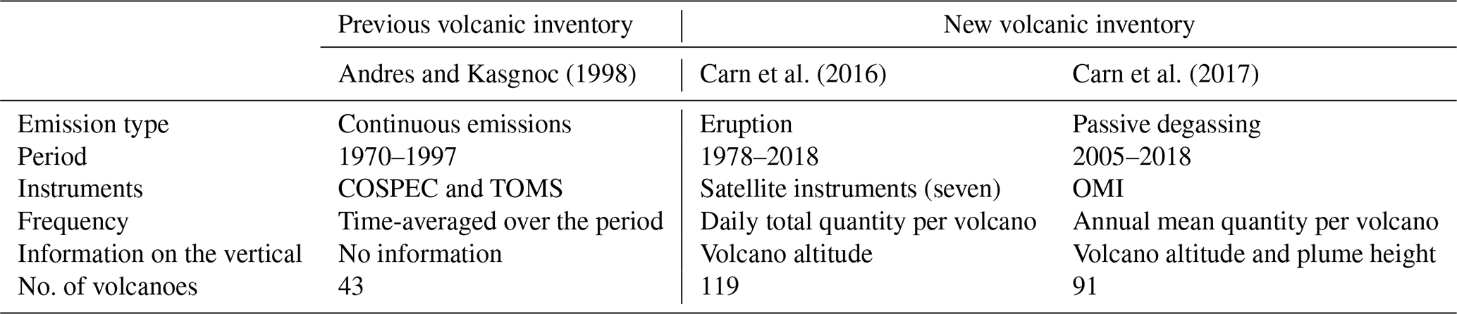
3.1 Previous volcanic sulfur inventory
The previous inventory implemented in MOCAGE is from Andres and Kasgnoc (1998), which is a study contributing to the work of GEIA (Global Emissions InitiAtive). Measurements ranged over a period of about 25 years, from the early 1970s to 1997, and covered volcanic SO2 emissions at the global scale.
A synergy between the COSPEC surface instrument and the TOMS satellite instrument was used. The COSPEC is a correlation spectrometer initially used in pollution measurements (Moffat and Millan, 1971; Williams-Jones et al., 2008). However, volcanologists have adapted it to measure the quantities of sulfur dioxide in a moving air mass (here the volcanic plume). It works by comparing the amount of solar ultraviolet (UV) radiation absorbed in the plume with a standard (one sample of the background sky and two laboratory-calibrated SO2 concentration cells). It is most commonly used under quiet to moderate eruptive conditions. On the contrary, the space instrument TOMS (Krueger et al., 1995; Seftor et al., 1997; Torres et al., 1998a), operational between 1978 and 2005, was able to detect larger eruptions. The synergy of these two instruments is therefore complementary in the development of the inventory. Although the first instrument is better adapted to the measurement of weak flares and the second to the strongest ones, a campaign dedicated to Popocatépetl in Mexico showed the good correlation between the two instruments (Schaefer et al., 1997).
Measurements were only carried out on sub-aerial volcanoes, i.e., emitting gases directly into the atmosphere. A total of 69 volcanoes are listed in the inventory, divided into two categories, namely 49 continuously erupting volcanoes and 25 sporadically erupting volcanoes. The following five volcanoes belong to both categories because they had a main activity of continuous emissions and also sporadic eruptive events: Mount Aso, Augustine, Kīlauea East Rift Zone, Mayon and San Cristóbal.
Since the beginning of volcanic emission measurements in the early 1970s, the global activity of continuous eruptions has shown relative stability. The fluxes provided in the inventory correspond to a temporal average of all measurements for each volcano. Only three volcanoes are not concerned by this hypothesis, i.e., Mount Etna in Sicily and Kīlauea and the Kīlauea Rift Zone in Hawaii, which are known as being among the largest emitters of SO2. For those volcanoes, fluxes provided by specific studies (Andres and Kasgnoc, 1998, personal communication) supersede the averages.
Since sporadic eruption data in Andres and Kasgnoc (1998) are not recent, it is not possible to take them into account for the recent year chosen for the MOCAGE simulation. Therefore, only continuous eruptions are used in MOCAGE and a global time-averaged SO2 flux of 13 Tg yr−1 is reported.
Since no configuration was developed in MOCAGE to inject volcanic emissions aloft until this study, they were implemented in a similar manner to the other pollution sources. Volcanic SO2 were thus emitted at the model surface (see Sect. 2.3). However, the surface elevation of the model (orography) is mainly below the actual elevation of the volcanoes.
3.2 New volcanic sulfur inventory
With the improvements in satellite technology, an increasing number of satellites are now able to better detect the sources of volcanic SO2, i.e., plume heights, quantities emitted and location. The most recent instruments with respect to TOMS, such as the Ozone Monitoring Instrument (OMI) and the TROPOspheric Monitoring Instrument (TROPOMI; Theys et al., 2019), have a higher sensitivity to detecting small eruptions but also passive degassing. Global coverage gives another considerable advantage over other measurement techniques. As a reminder, COSPEC carries out measurements from the ground and cannot be deployed on hard-to-access volcanoes.
The work of Carn et al. (2016, 2017) updates and adds complementary information to the study of Andres and Kasgnoc (1998) with a new inventory. The inventory is divided into two parts corresponding to the two types of emissions detectable by satellites.
First, the eruptive emissions data set (Carn et al., 2016, with data available in Carn, 2021) is a synthesis of 40 years of daily SO2 measurements (between 31 October 1978 and 31 December 2018) derived from the following seven satellite instruments: TOMS, OMI and OMPS (Ozone Mapping and Profiler Suite) in the ultraviolet (UV), TIROS Operational Vertical Sounder (TOVS), Atmospheric InfraRed Sounder (AIRS) and Infrared Atmospheric Sounding Interferometer (IASI) in the infrared (IR) and the Microwave Limb Sounder (MLS) in the microwave range. Data from 119 volcanoes and a total of 1502 events over the period are provided. For each of these eruptions, the information given includes the location of the volcano (latitude and longitude), the date, the VEI (Volcanic Explosivity Index), the estimated SO2 mass released (in kilotons) and also the height of the volcano and the height of the plume (measured if possible; estimated if not). Within our study, the additional information from Carn et al. (2016) on the injection height is used (see details hereafter), taking into account the height of the volcano as the base of the emissions and the height of the plume as the top of the injection.
Second, the passive degassing data set is the first documented volcanic sulfur dioxide emission inventory made with global satellite measurements (Carn et al., 2017). It was retrieved from the observations of the OMI instrument in the UV spectrum during a long-term mission between 2005 and 2015. The high sensitivity of the instrument was a technological breakthrough that made it possible to distinguish low SO2 sources; this means ∼30 kt yr−1 for persistent anthropogenic sources and lower amounts (∼6 kt yr−1) for volcanoes which are located at higher altitudes or at lower latitudes that benefit from more satellite observations and optimal conditions (low solar zenith angle). The volcanic SO2 sources have been identified on the basis of 3-year averages (2005–2007, 2008–2010 and 2011–2014), which implies that, for a source to be characterized as persistently degassing, the emission must be relatively constant on this timescale. Annual mean emissions were calculated for each of the 90 volcanic sources identified over the 11 years of the study. We assume in the model that emission fluxes are constant throughout the year.
Several parameters can affect the retrieval of volcanic emissions, namely the measurement process, the calculation algorithm or the characterization of the type of emission. Thus, annual uncertainties are given with the mean annual emissions for each volcano and each year. The total uncertainty of the annual sulfur dioxide fluxes are estimated at 55 % and over 67 % for sources emitting more than 100 and less than 50 kt yr−1, respectively. This latter information is exploited in the sensitivity analysis (see Sect. 8). Note also that, depending on the instrument used, the retrieval of the plume altitude can differ. Therefore, there are uncertainties on the altitude information provided by the inventory.
Information on the altitude of volcanoes and on the plume height in the Carn et al. (2016) inventory is used to implement a configuration to inject volcanic emissions aloft rather than keeping them at the model surface. This is an important improvement because, in some areas, depending on the model resolution chosen, the model orography may differ from the actual topography and have an impact on the transport of volcanic emissions. The new implementation sets the passively degassing emissions at the model level of the volcano altitude. For eruptions, the mass of SO2 emitted is distributed from the model level at the volcano vent to the model level of the plume top height and follows an umbrella profile similar to that used in other chemistry models (Freitas et al., 2011; Stuefer et al., 2013). During a volcanic eruption, the emitted materials (ashes and gases) are rapidly transported vertically by the convection in the plume, and most of the materials are concentrated at a high altitude, giving an umbrella profile. In practice, the plume follows an almost linear profile, with an increasing altitude from the volcano vent, and then it opens into a parabola containing 75 % of the gases in mass into the top third of the plume.
In summary (see Table 1), the updated volcanic sulfur emission inventory now includes about 160 volcanoes (∼110 in the eruptive category and ∼90 in the passive degassing category with 40 volcanoes in common). The availability of plume heights in this inventory allows a better representation of the injection of the volcanic emission in the model.
Andres and Kasgnoc (1998)Carn et al. (2016)Carn et al. (2017)Table 1Summary of the main characteristics of the previous (Andres and Kasgnoc, 1998) and the updated (Carn et al., 2016, 2017) SO2 volcanic emission inventories.
4.1 Description of the simulations
Meteorological fields are driven by the ARPEGE 3 hourly forecasts. Anthropogenic and biomass burning sources emit SO2, whereas biogenic emissions from the ocean are assumed to occur as DMS. Oceanic DMS emissions are 19.9 Tg S yr−1, while anthropogenic emissions are 48.6 Tg S yr−1. For 2013, biomass burning emissions from GFAS products were relatively low, at only 1 Tg S yr−1.
Concerning volcanic sulfur emission inventories, either Andres and Kasgnoc (1998) or Carn et al. (2016, 2017) is used. The full eruption emission database is available following Carn (2021, https://doi.org/10.5067/MEASURES/SO2/DATA405).
Andres and Kasgnoc (1998)Carn et al. (2016)Carn et al. (2017)Carn et al. (2016, 2017)Table 2Main features of the simulations.
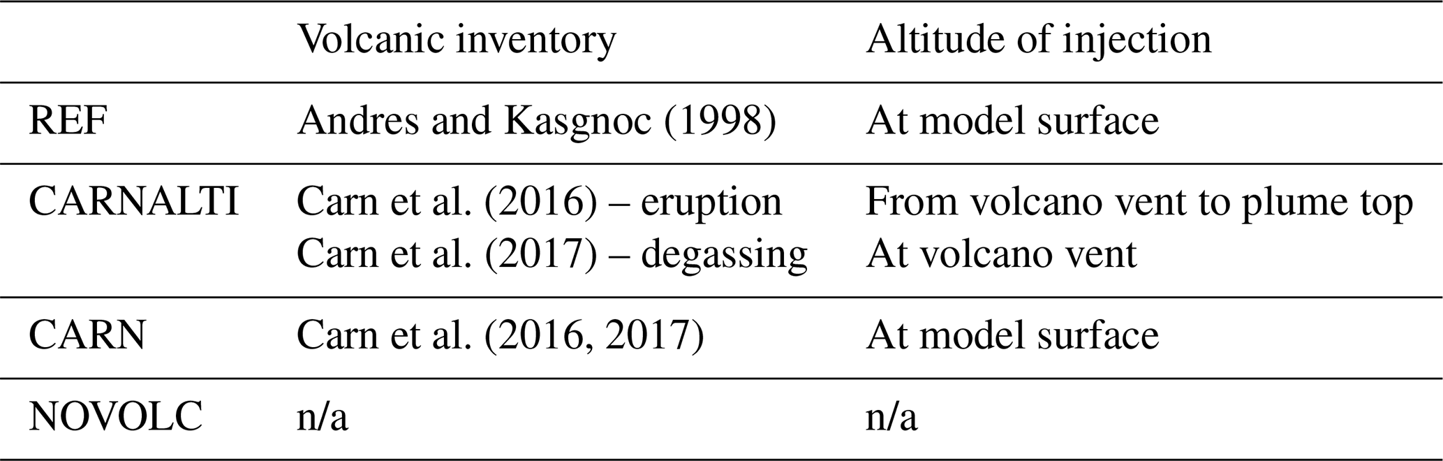
Note: n/a: not applicable.
In total, four different simulations (Table 2) are carried out in order to evaluate the impact induced by the update of the volcanic SO2 inventory in MOCAGE and to analyze its contribution to the sulfur species budget in the atmosphere at the global scale. The four simulations are run at a resolution of .
The first simulation, named REF, takes into account the previous volcanic inventory (from Andres and Kasgnoc, 1998) with the injection at the model surface. The second simulation, named CARNALTI, uses the updated volcanic inventory (from Carn et al., 2016, 2017) and the new configuration to inject volcanic emissions from the volcano altitude, as described in Sect. 3.2. By comparing REF and CARNALTI runs, we can analyze the changes brought by the updated volcanic emission inventory with respect to the previous one. These two simulations are evaluated in Sect. 5, and the associated global distribution of sulfur species is compared in Sect. 6.
In order to distinguish between the impact of the height of emission and of the quantity of SO2 emitted, another simulation, named CARN, is run and used for the analysis of the differences between the REF and CARNALTI global distribution of sulfur species. Volcanic emissions are from Carn et al. (2016, 2017), as in CARNALTI, but they are injected at the model surface, as in REF.
CARNALTI is run to provide a better representation of the global tropospheric sulfur. This is why it is selected for the analysis of the tropospheric sulfur budget in Sect. 7. In order to quantify the contribution of the volcanoes in the sulfur budget, we compare CARNALTI to the NOVOLC simulation that does not take into account volcanic emissions (only anthropogenic, biomass burning and dust).
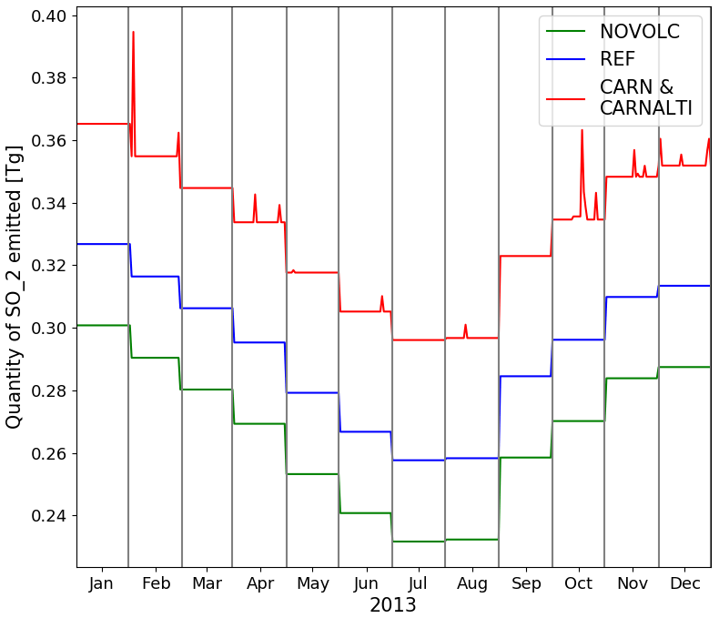
Figure 1Temporal evolution of 2013 SO2 emissions in Tg, the non-volcanic emissions inventory for NOVOLC, plus the Andres and Kasgnoc (1998) volcanic emissions inventory in REF or the Carn et al. (2016, 2017) volcanic emissions inventory in CARN and CARNALTI.
The four simulations are run for the year 2013 with a 3 month spin-up period (from October to December 2012). In addition to being one of the years for which a large amount of observational data is available globally, 2013 is chosen as the year with the lowest eruptive emission flux (Carn et al., 2016). Figure 1 shows the volcanic emissions of the different simulations for the year 2013. We notice the monthly variation due to non-volcanic emissions (NOVOLC run in green), with fewer emissions during the Northern Hemisphere summer and the highest values in the Northern Hemisphere winter. Volcanic emissions from Andres and Kasgnoc (1998) are steady throughout the year, as we can see in the REF run (in blue). They are lower than the volcanic emissions of the CARNALTI and CARN runs (in red), with strong constant passive degassing throughout the year and a few sporadically eruptive events. Indeed, Andres and Kasgnoc (1998) SO2 emissions are 13 Tg (or 6.5 Tg S), while the total 2013 annual emissions in Carn et al. (2016, 2017) are 23.7 Tg of SO2 (or 11.8 Tg S), with 23.5 Tg of passive degassing SO2 and 0.2 Tg of eruptive emissions (<1 % of the total amount of volcanic SO2 emissions, which is almost negligible).
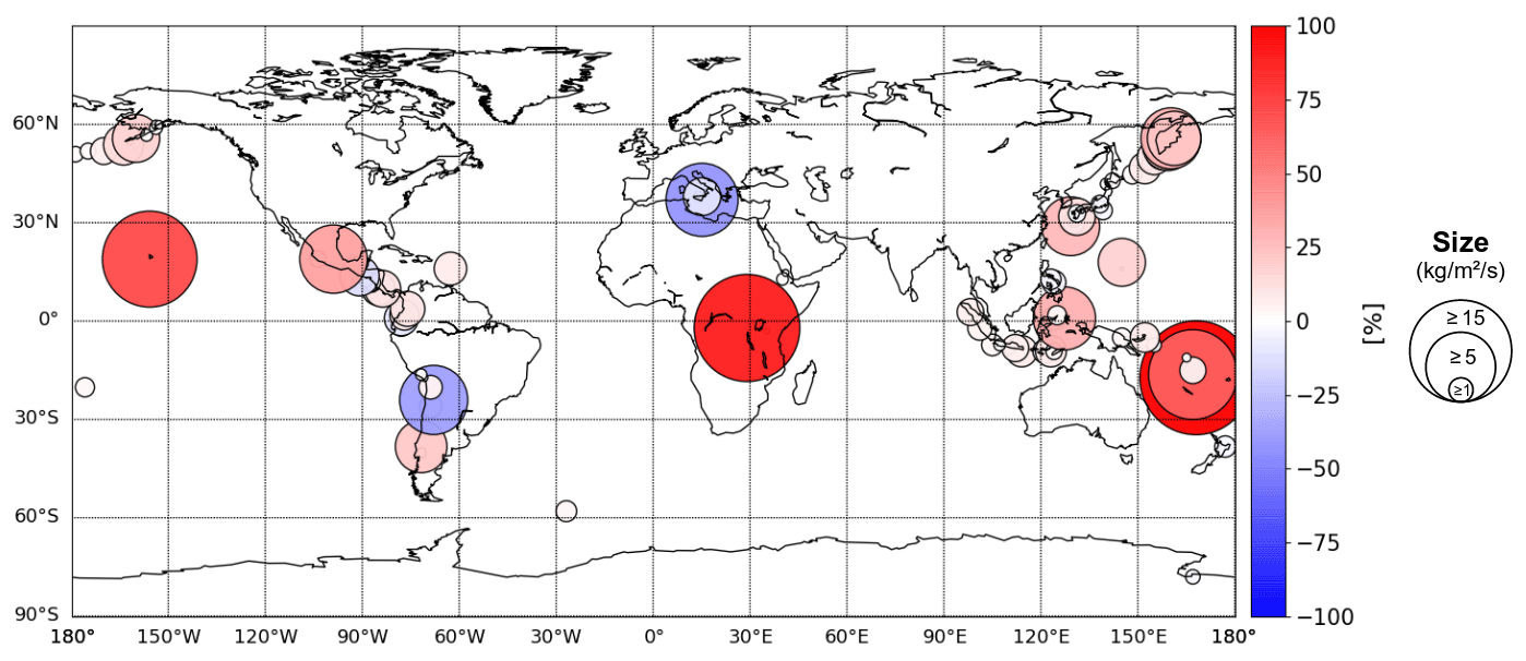
Figure 2The 2013 annual average ratio between volcanic SO2 emissions in the Carn et al. (2016, 2017) and Andres and Kasgnoc (1998) inventories. The size of the circles represents the absolute difference in kilograms per meter per second (), while the color represents the relative difference in percent.
Figure 2 spatially represents the difference between the previous and the new inventories. The red dots mostly show new volcanoes in Carn et al. (2016, 2017) which are not accounted for by Andres and Kasgnoc (1998). However, we also notice blue dots, meaning that, in the new inventory, the estimated emission fluxes are reduced. Given the low number of eruptive emissions in 2013, the annual average of volcanic emissions in Fig. 2 essentially represents passive emissions.
4.2 Observations used for the evaluation of the simulations
We use satellite-based instruments for the model evaluation since they provide a global sampling. The target chemical species that we evaluate are SO2 and aerosols, since SO2 is the precursor of sulfate aerosols. Concerning SO2, observations in the infrared are not suitable since passive degassing occurs mostly under 5 km, at altitudes where such instruments have reduced sensitivity (Carboni et al., 2012; Taylor et al., 2018). Therefore, observations in UV-visible range are chosen. With the Global Ozone Monitoring Experiment–2 (GOME-2) Metop-A (Meteorological Operational satellite) instrument being at the end of its lifetime, data retrievals are not good enough and present strong artifacts, as is the case for GOME-2 Metop-B. Therefore, we choose the OMI, which is the most widely used (e.g., He et al., 2012; Fioletov et al., 2013; Wang et al., 2017; Wang and Wang, 2020). Moreover, the SO2 tropospheric column estimated from the OMI is the finest resolution and most accurate instrument from 2013 for retrieving SO2 total columns over passively emitted volcanoes with altitudes that are generally around 2–3 km. For aerosols, there is no satellite-derived product providing information on sulfate only. Nevertheless, satellite observations of aerosols as a whole are available. Here, we choose MODIS (Moderate-Resolution Imaging Spectroradiometer) aerosol optical depth (AOD), which provides data at the global scale. MODIS AOD is known as being a robust product and is used in the literature for global evaluation and aerosols assimilation in models (e.g., Liu et al., 2011; Dai et al., 2014; Sič et al., 2015; Guth et al., 2016, 2018). The model comparison with MODIS AOD provides an indirect evaluation for sulfate aerosols since AOD includes sulfate aerosols.
4.2.1 OMI SO2 total column
The Aura Ozone Monitoring Instrument (OMI) level 2 sulfur dioxide (SO2) total column product (Li et al., 2020) was used to validate the model simulations. This product has been available since 2004. The resolution of the data is 13 km×24 km at the nadir. The retrieval algorithm is a principal component analysis (PCA)-based algorithm (Li et al., 2013). Various physical and technical causes can reduce the quality of data. Thus, pre-processing and data filtering were applied as recommended to select only the best possible observations. Pixels with large solar zenith angles (SZAs>65∘), affected by the South Atlantic Anomaly region (Richter et al., 2006), on the edge of the swaths or the OMI row anomaly (signal suppression at certain OMI rows; see Schenkeveld et al., 2017) and pixels with a cloud fraction greater than 30 % or flagged with low-confidence data are removed.
There are various products available in the OMI data set since the OMI instrument has a variable sensitivity, depending on altitude, and the retrieval of SO2 requires the use of an a priori profile. The first product selected, named Column_Amount_SO2, is an estimate of SO2 vertical column density (VCD) and constrained by the GEOS-5 global model a priori profiles. Then, three specific products with adapted a priori profiles are also available and selected. One, named Column_Amount_SO2_PBL, is an estimate of the SO2 vertical column density (VCD), with an a priori profile assuming that the essence of SO2 is in the boundary layer (within the lowest 1 km of the atmosphere). Another product, named Column_Amount_SO2_TRL, is almost the same as the previous one but assumes a lower tropospheric SO2 profile (with a center of mass altitude at 3 km). The last product selected, named Column_Amount_SO2_TRM, corresponds to an assumed middle tropospheric SO2 profile (with a center of mass altitude at 8 km).
4.2.2 MODIS aerosol optical depth
We use daily level 3 MODIS data (MOD08, Terra; MYD08, Aqua; collection 6.1) for the year 2013. Before use, we performed additional quality control and screening (Sič et al., 2015; Guth et al., 2016). These treatments aim at minimizing cloud contamination and avoid low-confidence measurements (Zhang et al., 2005; Koren et al., 2007; Remer et al., 2008). Moreover, all AOD values below 0.05 are automatically filtered out because Ruiz-Arias et al. (2013) highlighted the rapid growth in the relative underestimation of AODs after this threshold, which leads to a mean relative error above 50 %.
In MOCAGE, AODs are calculated using Mie theory with the Global Aerosol Data Set's refractive indices (Köpke et al., 1997) and extinction efficiencies derived with the Mie scattering code for homogeneous spherical particles from Wiscombe (1980).
4.3 Statistical metrics used for evaluation
In order to evaluate the model against observation data, we use the fractional bias, the fractional gross error, the root mean square error and the correlation coefficient, following Seigneur et al. (2000).
The fractional bias or modified normalized mean bias (MNMB) quantifies the mean between the modeled (f) and the observed (o) elements, for N observations. It ranges between −2 and 2 and varies symmetrically with respect to the under- and overestimation of the model. The definition is given by the following:
The fractional gross error (FGE) quantifies the model error. It is a positive variable ranging between 0 and 2. The definition is given by the following:
The root mean square error (RMSE) is the square root of the average of the squared difference between each model and observation value. In other words, it represents a measure of the accuracy in absolute values, while FGE is relative. RMSE is a positive variable, and a value of 0 (almost never achieved in practice) would indicate a perfect fit to the data. The formula is given by the following:
The correlation coefficient (R) indicates whether the variations in the model and the observations are well matched and ranges between −1 and 1. The closer the score is to 0, the weaker the correlation is. The definition is given by the following:
where and are, respectively, the model and observations mean values, and σf and σo are the standard deviations from the modeled and observed time series.
5.1 Evaluation strategy
For the evaluation of the simulations, OMI and the MODIS data set are mapped at the model resolution (). The model grid points in the simulations corresponding to the filtered observation pixels (as explained in Sect. 4.2.1 and 4.2.2) are also removed. A different validation strategy is applied, depending on the instrument.
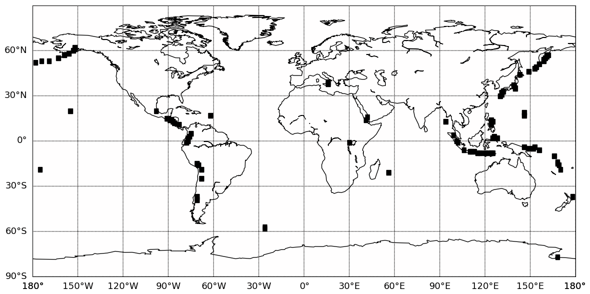
Figure 3Location of the selected areas where OMI SO2 total column are selected for the validation. They correspond to nine MOCAGE grid points around each volcano from Carn et al. (2016, 2017).
Concerning OMI SO2 total columns, similarly to other SO2 satellite-derived products, their relative uncertainties are large where the signal is low, in particular for background conditions. This is why, in the literature, the SO2 satellite comparisons and the model evaluations focus on specific areas close to SO2 sources (e.g., He et al., 2012; Fioletov et al., 2013; Wang and Wang, 2020). Similar to these studies, our strategy is to perform the model evaluation only in the vicinity of the volcanic sources. For each volcano, based on those referenced in Carn et al. (2016, 2017), we select nine model grid points (representing a square of ), with the middle point being where the volcano is located (see Fig. 3). Altogether, it corresponds to 633 points. The mask is applied on each daily OMI SO2 total column measurements, and then we perform an annual average for each of the 633 data points. Similar to the abovementioned studies, the results are shown as scatterplots, and the statistical metrics used are the correlation coefficient and the RMSE.
In total, two methods are used in the evaluation strategy. First, we choose to evaluate the model SO2 total column against OMI Column_Amount_SO2 product. However, in order to test if the evaluation is sensitive to this choice, we use another approach which consists of an interpolation of OMI SO2 observations at the altitude where the volcanic emissions are injected in MOCAGE. To do so, we use the OMI products Column_Amount_SO2_PBL, Column_Amount_SO2_TRL and Column_Amount_SO2_TRM, hereafter renamed PBL, TRL and TRM, respectively. Depending on the altitude of the emissions in MOCAGE, either PBL and TRL or TRL and TRM are used for the interpolation.
Concerning the AODs, a spatial validation on the whole global domain is possible against MODIS products. The evaluation at the global scale enables us to quantify the overall aerosol changes in the simulations from the use of the updated inventory with respect to the previous one. Since noticeable changes are also expected at the local scale in the vicinity of the volcanoes, three zones are selected to complete the global-scale evaluation against MODIS. These zones are chosen from among the largest passive SO2 emitters in Carn et al. (2017) and are representative of different types of changes between Andres and Kasgnoc (1998) and Carn et al. (2016, 2017) volcanic emissions inventories.
Zone 1 is centered over central Africa and is under the influence of Mount Nyiragongo and Nyamuragira (altitude of 2950 m). In Andres and Kasgnoc (1998), this volcano is not listed. In contrast, in Carn et al. (2017), the passive degassing emission represents 2.29 Tg in 2013. No eruption is listed in Carn et al. (2016) for 2013.
Zone 2 is located in the northern Pacific Ocean around Hawaii. The volcano, based on the island, is Kīlauea (altitude of 1222 m). In the REF simulation, the volcano emissions in the inventory are 0.45 Tg yr−1 (seventh rank of the most SO2-emitting volcanoes in Andres and Kasgnoc, 1998). But, in Carn et al. (2017), the Kīlauea emissions are updated, and it is the second-biggest emitter, with 2.17 Tg. In 2013, no eruptions are recorded in Carn et al. (2016) for this area.
Zone 3 is located in the Mediterranean region, under the influence of Mount Etna (altitude of 2711 m in the inventory) and Stromboli (altitude of 870 m in the inventory). In Andres and Kasgnoc (1998), 1.48 Tg yr−1 is emitted by Mount Etna (the biggest volcanic SO2-emitter referenced), 0.27 Tg yr−1 is emitted by Stromboli and also 0.02 Tg yr−1 by Vulcano. In Carn et al. (2016, 2017), only 0.65 Tg of SO2 are emitted in 2013 in zone 3, corresponding to less than 0.04 Tg for Stromboli and 0.61 Tg for Mount Etna. Vulcano is not in the Carn et al. (2016, 2017) inventories. In 2013, small eruptions occurred at Mount Etna, totaling a little less than 0.06 Tg. Therefore, in the updated Carn et al. (2016, 2017), volcanic emissions in zone 3 are weaker than in Andres and Kasgnoc (1998).
For the evaluation of the simulations against MODIS, the statistical metrics used are the MNMB, FGE and correlation coefficient. Because MNMB and FGE are dimensionless, they are meaningful in all geographical regions regardless of the magnitude of the aerosol column.
5.2 Validation against OMI SO2 total column
Figure 4a presents the scatterplots of MOCAGE SO2 columns in DUs (Dobson units) from the REF and CARNALTI simulations against OMI observations based on GOES-5 a priori profiles. Each of the points represents an average over the 2013 year. It shows that the previous version of the model (REF) was not good. The correlation coefficient is low (0.13). The bias is high, with a mean SO2 measured by OMI of 0.28 DU and of 0.11 in REF simulation. With the new volcanic inventory in the CARNALTI simulation, the mean SO2 concentration is similar to OMI retrievals (0.27). We can also clearly see an improvement of the model performances with a correlation increased up to 0.67.
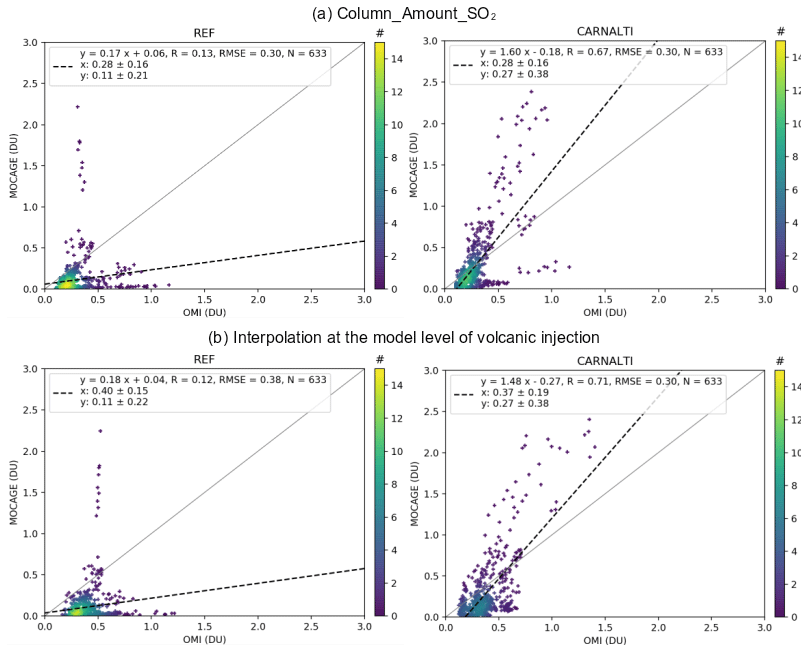
Figure 4Scatterplots of annual mean OMI SO2 versus MOCAGE simulations (left – REF; right – CARNALTI) (a) considering total columns and (b) interpolating at the model level where volcanic emissions are injected. Also shown are the 1:1 line (solid gray), linear regression line (black dash), linear regression formula, correlation coefficient (R), root mean squared error (RMSE), number of collocated pairs (N), OMI mean and standard deviation in DU (x), MOCAGE mean and standard deviation in DU (y) and density of collocated pairs (color bar).
To evaluate the impact of the choice of OMI product, we also show in Fig. 4 (bottom row) the scatterplot when applying the interpolation at the MOCAGE altitude where volcanic emissions are injected. This method provides higher OMI estimates and, therefore, increases the bias with MOCAGE simulations, but it improves the correlation. The conclusion is that the CARNALTI simulation provides by far better statistical results (bias, RMSE and correlation) than REF. The negative bias of MOCAGE CARNALTI with respect to OMI could be due to errors in the plume transport in the model linked to uncertainties in the meteorological inputs, to the limited number of model vertical levels, to the model chemistry and/or aerosol scheme or also to the uncertainties in the SO2 emission estimates from OMI in Carn et al. (2016, 2017) and in the OMI retrieval products used for the model evaluation.
Validation against MODIS AOD at 550 nm
As a second evaluation step, we compare the simulations' AOD with the AOD from MODIS. Figure 5 presents, for the REF and CARNALTI experiments, the 2013 annual MNMB with respect to MODIS AOD observations. We can see that the equatorial belt has a negative MNMB, between −0.2 and −1.2 in the REF simulation, but in the CARNALTI simulation, it is closer to 0; e.g., in the vicinity of volcanoes in Indonesia or in central Africa. This shows an improvement in the MOCAGE AOD modeling at the global scale by updating the volcanic emissions inventory. Despite the improvement in MNMB in the areas near volcanoes, the overall score is not improved (see Table 3). Indeed, the MNMB of the Northern Hemisphere is mainly positive and almost unchanged with the new inventory (Carn et al., 2016, 2017) in which only a few volcanoes are reported. Even this small number of volcanoes, locally, leads to an increase in the already positive MNMB. Thus, globally, the average MNMB is higher in CARNALTI than in REF.
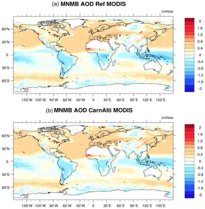
Figure 5Maps of the 2013 annual MNMB of aerosol optical depth against MODIS monthly observations for (a) REF and (b) CARNALTI simulations.
Table 3The 2013 annual statistics of the REF and CARNALTI simulations against MODIS observations on specific zones.

Concerning the fractional gross error (FGE), changes are also located in the vicinity of volcanoes (see Fig. S1 in the Supplement). In those areas, especially in central Africa and in Indonesia, the FGE is reduced from a maximum of 1.2 in REF to a maximum of 0.6 in CARNALTI. Globally, the FGE score is slightly improved, with 0.43 for REF and 0.42 in CARNALTI. Even if, locally in the Northern Hemisphere (e.g., in Hawaii), the FGE score can be deteriorated in the simulation with Carn et al. (2016, 2017), at the global scale, the new inventory is better.
The correlation coefficient R score is better in the Northern Hemisphere (see Fig. S1). Therefore, by adding new volcano point sources, and mostly in the Southern Hemisphere, the scores are higher in CARNALTI. The lifetime of aerosols increases when located in a higher altitude. Aerosols are better represented in the CARNALTI simulation thanks to the use of a better injection altitude of SO2 (a precursor of sulfate aerosols contributing to the AOD).
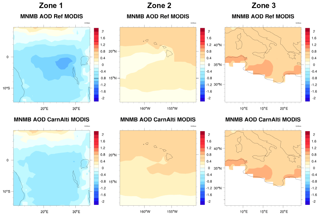
Figure 6Maps of the 2013 annual MNMB of the REF and CARNALTI simulations against MODIS observations at the specific zones.
By using Carn et al. (2017), the model results are improved in zone 1. The MNMB rises from −0.47 with the REF simulation to −0.34 in the CARNALTI run. Similarly, the FGE is improved. In Fig. 6 (left column for zone 1), the negative MNMB score in the REF simulation highlights the lack of the Nyamuragira volcanic SO2 emissions. The MNMB is largely reduced in CARNALTI simulation.
In zone 2, unlike the previous area, the MNMB is already positive. Thus, by adding more SO2 volcanic emissions, it increases the sulfate aerosol content, leading to a deterioration of the MNMB and FGE scores (Table 3). The correlation coefficient increases due to a more accurate altitude where the emissions are injected in the CARNALTI simulation. Figure 6 in the middle column confirms these results. However, with the volcano being located at an altitude of 1222 m, where the sensitivity of, mostly, infrared but also ultraviolet instruments is reduced, the estimation in the inventory for this volcano may be overestimated.
In zone 3, the statistical scores are almost similar for the two simulations. Indeed, in this region there are various other aerosols sources (industries, transport, dust, etc.), and sulfate from volcanic emissions does not dominate. Still, we can see, in Fig. 6, a small improvement in MNMB between the REF and CARNALTI simulations. The FGE and correlation scores are also a bit better in CARNALTI. Thus, using Carn et al. (2016, 2017) and injecting volcanic emissions at the actual altitude of the volcanoes slightly enhances MOCAGE performances.
5.3 Summary of the evaluation
The evaluation of MOCAGE performances against the OMI SO2 total column and MODIS AOD shows an improvement in the CARNALTI simulation compared to REF. The previous inventory (Andres and Kasgnoc, 1998) lacks some volcanic sources, which leads to a global underestimation of sulfur dioxide concentrations and aerosol concentrations in the tropics (e.g., in zone 1). With the new inventory (Carn et al., 2016, 2017) used in the CARNALTI simulation, volcanic emissions are larger. Even if in some areas the scores are deteriorated, e.g., in zone 2 where the model is already overestimating aerosol concentrations, the scores at the global scale and in the vicinity of most of the volcanoes are improved.
SO2, sulfate aerosols and PM2.5 tropospheric column and surface concentrations are summarized in Table 4. In order to dissociate the effect of the quantity of SO2 emitted and of the injection altitude, we compare the REF and CARNALTI simulations with the CARN run. The annual mean sulfur dioxide total column, at the global scale, is mol m−2 in the CARNALTI simulation, which is 13 % higher than the mol m−2 in REF. Regarding aerosols species, sulfate total column is 23 % higher in the CARNALTI simulation, but only by 1 % for PM2.5, because it is only partially composed of sulfate. This increase is explained by the greater amount of SO2 emitted in Carn et al. (2016, 2017) and by the new injection configuration. At higher altitudes, the lifetime of sulfur species is longer due to slower removal processes (Stevenson et al., 2003). Figure 7 illustrates this concept. It shows the relative difference in the sulfate tropospheric column between the CARNALTI and REF experiments. We clearly see an increase in CARNALTI concentrations in the vicinity of most volcanic point sources.
Table 4Global and local (zones 1, 2 and 3) 2013 annual mean concentrations in the REF, CARN and CARNALTI simulations. Gases are in moles and aerosols in kilograms.

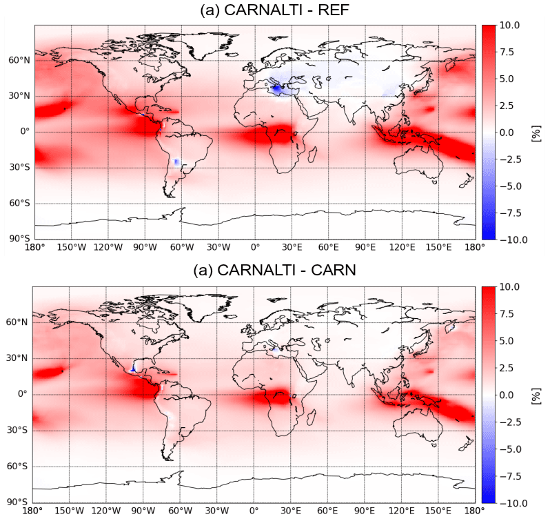
Figure 7The 2013 annual mean sulfate tropospheric column relative difference between the (a) CARNALTI and REF simulations and the (b) CARNALTI and CARN simulations (in percent).
Surface concentrations, at the global scale, from the simulations show different results. With kg m−3 in the REF simulation, sulfate is lower than in the CARNALTI simulation, with kg m−3 (+8 %). However, concerning SO2 surface concentrations, with mol m−3, there is more SO2 in the REF than in the CARNALTI simulation, with only mol m−3. Even if there are more volcanic SO2 emissions in the CARNALTI run, by injecting it in altitude, sulfur dioxide remains in the atmosphere longer and reaches the surface less. But, in the CARN simulation results, where the volcanic emissions are injected at the model surface, we notice higher concentrations of SO2 at the surface ( mol m−3). The mean sulfate aerosol concentrations in the CARN simulation are kg m−3. This is 4 % higher than in the REF simulation (as seen before) but also almost 4 % lower than in the CARNALTI simulation. Indeed, compared to REF, with more volcanic emissions, there is more formation of sulfate (such as in the CARNALTI run). However, due to being emitted at the surface, sulfate aerosols are rapidly removed by deposition in CARN compared to CARNALTI. Figure 7 shows this difference in the transport of sulfate aerosols. In the CARNALTI simulation, we can clearly see the volcanic plumes spreading further from the volcanoes, almost 150 to 200 km away.
By looking at the local scale, the differences between CARNALTI and REF can be very large. For example, in zone 1, the SO2 tropospheric column is 3 times larger in CARNALTI (from mol m−2 in REF to mol m−2), 2 times larger for the aerosol sulfate total column (from to kg m−2) and almost twice as large for sulfate at the surface ( to kg m−3). In zone 2, changes are also more important compared to the global scale, with 77 % more concentration of SO2 and 53 % higher concentration of sulfate in the atmosphere and 23 % more sulfate at the surface. In zone 3, there is less impact because it is a more polluted area.
The difference between CARN and CARNALTI SO2 and aerosol sulfate tropospheric columns are not as important as between REF and CARNALTI. Sulfur species concentrations are highest in CARNALTI compared to CARN, with the exception of SO2 in zone 3. In this highly polluted area, anthropogenic emissions are dominant. The volcanic SO2 emitted is then more likely to compete with SO2 from other sources, leading to an increase in its lifetime. At the surface, as expected, the SO2 concentration is much higher in all zones in the CARN simulation compared to CARNALTI (e.g., 51 % smaller in zone 2 in CARNALTI compared to CARN). However, for sulfate aerosols, the surface concentrations are higher in the CARNALTI run compared to CARN in zones 1 and 2. With volcanic emissions injected into the upper levels of the model, the lifetime of SO2 increases and more sulfate aerosols are formed (as we can see in the tropospheric column), more sulfate is found near the surface.
Concerning particulate matter, the impact of Carn et al. (2016, 2017) at the global scale does not present significant changes (in both the tropospheric column and at the surface) because PM2.5 is not composed only of sulfate aerosols but is the sum of all the atmospheric aerosols with a diameter less than 2.5 µm. However, we found larger changes locally; e.g., 10 % higher PM2.5 tropospheric column concentration in CARNALTI, with kg m−2, compared to REF, with kg m−2, in zone 1. As expected, for zone 3, all chemical species concentrations are smaller in CARNALTI compared to the REF simulation, especially at the surface.
In this section, we calculate the MOCAGE sulfur budget and analyze the impact of the new volcanic SO2 emissions on the tropospheric species distribution with the CARNALTI run. In order to isolate the contribution of volcanic emission from the other species concentration, we look at the difference between CARNALTI and NOVOLC simulations. The relative contribution of volcanic SO2 emissions to the species budget is defined by the quantity of species in the CARNALTI simulation subtracted from the quantity of species in the NOVOLC simulation, with respect to the total quantity of species in the CARNALTI simulation, in the following:
with XCARNALTI and XNOVOLC being the annual mean concentration of the parameter X in CARNALTI and NOVOLC simulations, respectively.
Hereafter, the parameters from NOVOLC simulation will be named non-volcanic parameters. On the contrary, volcanic parameters correspond to the parameters of the CARNALTI simulation minus the quantity in the NOVOLC simulation. The CARNALTI simulation represents the total (volcanic + non-volcanic) concentration of the parameters.
7.1 Global budgets
The global sulfur budget simulated in CARNALTI is shown in Table 5. Annually and globally averaged SO2 emissions, SO2 and sulfate aerosols burdens, as well as sulfur wet and dry depositions, are used to calculate the sulfur budget.
Table 5The 2013 annual global mean SO2 emissions, sulfur budget and deposition quantities (in teragrams). The contribution of sulfur species due to volcanic emissions or other emission sources are presented (in percent). The efficiency is the ratio between the contribution of the sulfate burden and the contribution of the total sulfur emission attributed to a specific source. In other words, it is the fractional contribution from anthropogenic and volcanic sources to the sulfate burden. Note: sedim – sedimentation.
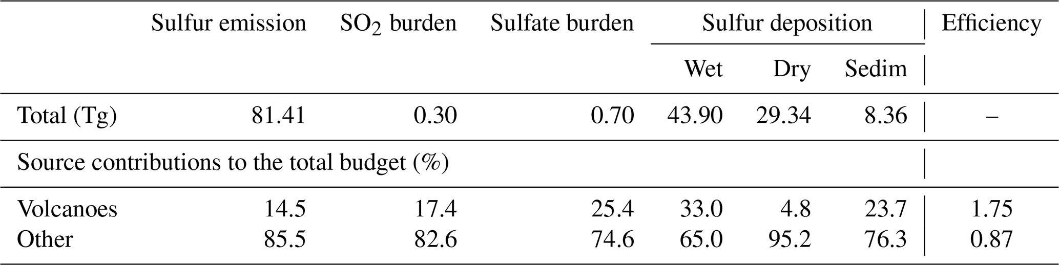
Volcanic emissions are 11.8 Tg yr−1. This estimation remains in the range of previous studies which estimated volcanic emissions to be between 7 and 14 Tg (Berresheim and Jaeschke, 1983; Chin and Jacob, 1996; Graf et al., 1997; Sheng et al., 2015, updated in Feinberg et al., 2019). However, due to lower anthropogenic emissions compared to those studies because of the recent year chosen (2013), the 15 % contribution from volcanic emissions to the total sulfur emissions in CARNALTI is higher.
The global SO2 burden is 0.30 Tg, similar to other studies whose values range from 0.2 to 0.52 Tg (Pham et al., 1995; Chin and Jacob, 1996; Feichter et al., 1996; Graf et al., 1997; Stevenson et al., 2003; Feinberg et al., 2019). In our simulation, 34.69 Tg S are directly removed by the dry and wet deposition of sulfur dioxide, representing a percentage of almost 43 %. Thus, the transformation rate of SO2 to sulfate is about 57 %, which is consistent with the studies reported above (from 50 % to 66 %).
The global vertical sulfate column is 0.70 Tg S, comparable with other studies, i.e., 0.53 Tg S in Chin and Jacob (1996), 0.78 Tg S in Graf et al. (1997), 0.81 Tg S in Stevenson et al. (2003) and 0.64 Tg S in Feinberg et al. (2019).
These results confirm the nonlinear contribution of the different SO2 sources emissions to the sulfate burden. Indeed, volcanic sources represent almost 15 % of the total SO2 emitted into the atmosphere, but they contribute 25 % to the sulfate burden. The transformation of SO2 into sulfate from the other sources is not as efficient. We can note a higher efficiency for the volcanic sources, at around 1.75, compared to the other sources, at 0.87.
The total sulfur deposition is around 82 Tg S, including 35 Tg S of SO2, a little less than the total sulfur deposition in Feinberg et al. (2019) of 94 Tg S, and also including 22 Tg S of SO2. The difference comes from the aerosol deposition which depends on the deposition scheme and the meteorological fields, which can vary depending on the considered time period. In our study, the sulfur deposition is mainly wet deposition. Precisely, the partitions of each deposition flux are 55 % for wet deposition, 35 % for dry deposition and 10 % from sedimentation. But sulfur deposition due to volcanic emissions is weaker than for the other sources, i.e., 35 % for wet deposition, 24 % for sulfate aerosol sedimentation and only 5 % for dry deposition. Due to the higher altitude of injection, the atmospheric residence time for volcanic sulfur species is longer, and the deposition rate is lower, especially for the dry deposition. Even though there is a lower contribution, we still note the strong contribution of volcanoes to wet deposition and sedimentation, which is much greater than the contribution to the emissions.
7.2 Vertical distribution
Figure 8 shows the global and annually averaged vertical profiles for sulfur dioxide and sulfate concentrations for 2013. Anthropogenic and volcanic sources are separated to highlight the main differences between them.
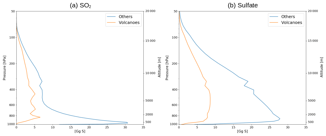
Figure 8The 2013 annual global mean vertical profile for (a) SO2 and (b) sulfate aerosols from volcanic and other sources.
Non-volcanic SO2 dominates the entire vertical column, with a maximum at the surface linked to anthropogenic emissions emitted at the model surface. On the contrary, the vertical distribution from volcanic SO2 shows variations. There is no contribution below 950 hPa, but there are three maxima above, i.e., one at 850 hPa (about 1500 m), due mostly to passive degassing, another around 680 hPa (about 3300 m), due to passive degassing from high-altitude volcanoes and eruptions, and the last one around 450 hPa (about 6000 m), due to high-altitude eruptions. It is noteworthy that, even with few eruptive events during the year 2013, the volcanic SO2 vertical distribution is affected by them.
Concerning sulfate aerosols, volcanic emissions are also not dominant over the entire vertical column. Non-volcanic sulfate aerosol have the highest values, around 950 hPa, near the surface. For volcanic sulfate, the maximum is between 850 and 450 hPa but 4 times smaller than for other sources and without any specific peak associated to passive degassing or eruptive emissions. These results are different from Graf et al. (1997), which shows that the vertical distribution of volcanic sulfate aerosols is comparable to anthropogenic and biomass burning sulfate and is even dominant between 800 and 300 hPa (the altitude of volcanic emissions, mainly from eruption). This difference between our study and Graf et al. (1997) can be explained by the quantity of SO2 emitted by eruptions. In 2013, only a few eruptive events occurred, while almost 30 % of volcanic emissions in Graf et al. (1997) are eruptive. Therefore, with a greater volume of volcanic emissions injected at higher altitude in Graf et al. (1997), the potential to form sulfate aerosols is greater than in our study. This can explain the greater efficiency of 2.63 in the tropospheric sulfate burden in Graf et al. (1997) compared to 1.75 in our study.
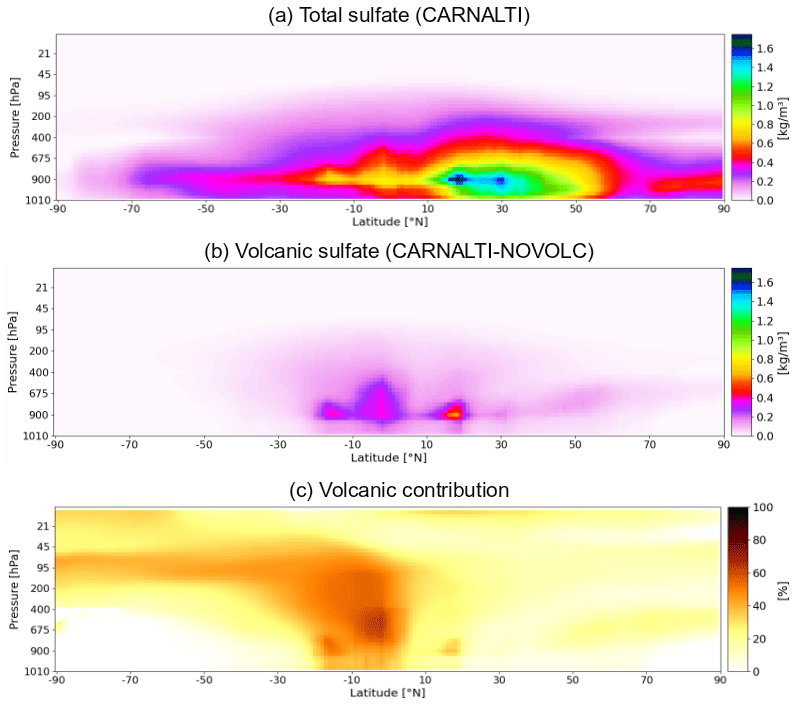
Figure 9The 2013 annual zonal mean (a) total sulfate concentration (in kilograms per cubic meter, hereafter kg m−3), (b) volcanic sulfate concentration (in kg m−3) and (c) volcanic sulfate contribution (in percent).
Figure 9a represents the annual zonal mean sulfate concentration. Most of the sulfate aerosols reside in the Northern Hemisphere (between 15 and 30∘ N) due to anthropogenic influence, and the highest values are around 800 hPa. The sulfate concentrations due to volcanic emissions (Fig. 9b) are located at higher altitudes. On both sides of the Equator, volcanic sulfate is found between 900 and 650 hPa. Over the tropical region, the volcanoes' contribution to the sulfate aerosol concentrations is larger, with a maximum of 50 %–60 % around 650 hPa (see Fig. 9c). We also notice that sulfate aerosols are transported by the general atmospheric circulation, up to the UTLS (upper troposphere lower stratosphere) and even into the stratosphere and from the Equator to the poles, especially in the Southern Hemisphere where there are more volcanoes.
7.3 Regional distributions
The volcanic contribution to the global surface SO2 concentrations is relatively low, around 2 %, but it is much higher close to the source points (see the top of Fig. 10 for SO2). This is mainly due to the high altitude of emissions from volcanoes. Similarly, Fig. 10 (bottom for sulfate aerosol) shows a greater influence of volcanic emissions on the sulfate aerosol concentration at the surface, which is almost larger than other sources in the vicinity of volcanoes. Globally, the mean contribution is of 10 %, but with a rather low, almost zero, contribution over continental areas in the Northern Hemisphere. Considering that, within the boundary layer, anthropogenic SO2 emissions are dominant, the sulfate aerosols formed in this environment come largely from anthropogenic rather than from other sources. However, in areas with small anthropogenic sources (Indonesia, Hawaii and central Africa), the volcanic contribution is large.
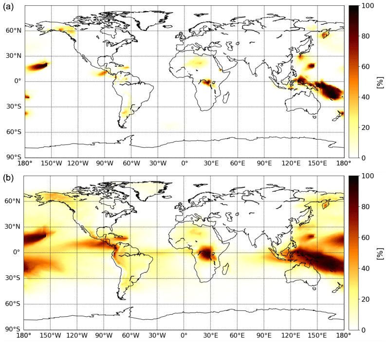
Figure 10The 2013 annual mean (a) SO2 and (b) sulfate surface contribution due to volcanic emission (in percent).
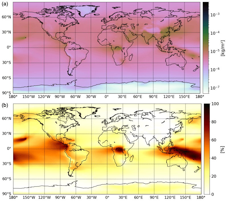
Figure 11(a) The 2013 annual mean sulfate tropospheric column from CARNALTI (in kilograms per square meter) and (b) its contribution due to volcanic emissions (in percent).
For the total column, volcanic emissions contribute a great to the sulfur species burden, i.e., 12 % to SO2 and 19 % to sulfate aerosols. In Fig. 11, we can see that the highest sulfate burden is located over polluted areas (eastern North America, Europe, the Middle East, India and China) and near some volcanoes and particularly over oceanic volcanoes. By looking at the volcanic contribution, we note that the sulfate aerosols due to volcanic emissions are mainly distributed over the oceanic environment in the tropics (also corresponding to volcanoes of lower altitudes). The highest contribution, 85 %, is found over Indonesia.
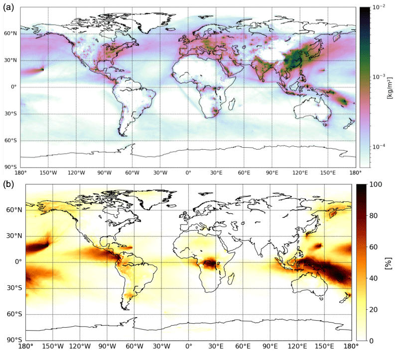
Figure 12(a) The 2013 annual mean sulfur deposition from CARNALTI (in kilograms per square meter) and (b) its contribution due to volcanic emissions (in percent).
The annual global depositions of sulfur species due to volcanic emissions are 23 %, 11 % and 10 % for wet deposition, dry deposition and sedimentation, respectively. Figure 12 represents the total sulfur deposition at the global scale and shows higher deposition fluxes over anthropogenic polluted areas, where volcanic contribution is low (see Fig. 12b). The only exception, where there are a high deposition flux and a high volcanic contribution, is Indonesia. Details on the proportion of each type of deposition (wet, dry and sedimentation) are shown in Fig. S5, where we notice a weak influence of sedimentation, consistent with Table 5, compared to wet and dry depositions.
Carn et al. (2017) provide for passive degassing not only for the annual SO2 volcanic emissions (, where V is the volcano and Y is the year) but for also the associated annual emission uncertainties (UV,Y) for each volcanic source. Thus, in this section, we aim at using this information to check the variability induced in the MOCAGE sulfur budget and to analyze how it affects our conclusions from the previous section.
8.1 Description of the supplementary simulations
In total, three additional simulations are conducted to analyze the sensitivity of the MOCAGE model to the uncertainty of volcanic passive emissions. The first one, named CA_MIN, takes into account, for each volcano, the lowest estimation of SO2 emissions. In other words, for each volcano, we remove the annual emission uncertainty to the annual mean emission as follows: . In contrast, the second simulation, named CA_MAX, takes into account the highest estimation of SO2 emission; we add the annual emission uncertainty to the annual mean emission as follows: . Thus, both CA_MIN and CA_MAX experiments do not have daily variations due to passive degassing but only due to eruptions. For the last one, named CA_RAND, emissions are randomly determined on a daily basis within the annual emission uncertainty interval, , following a continuous uniform distribution. Thus, daily variations are not only due to eruptions but also to passive degassing, as expected in reality. The reference simulation used, CARNALTI, is called CA from now on.
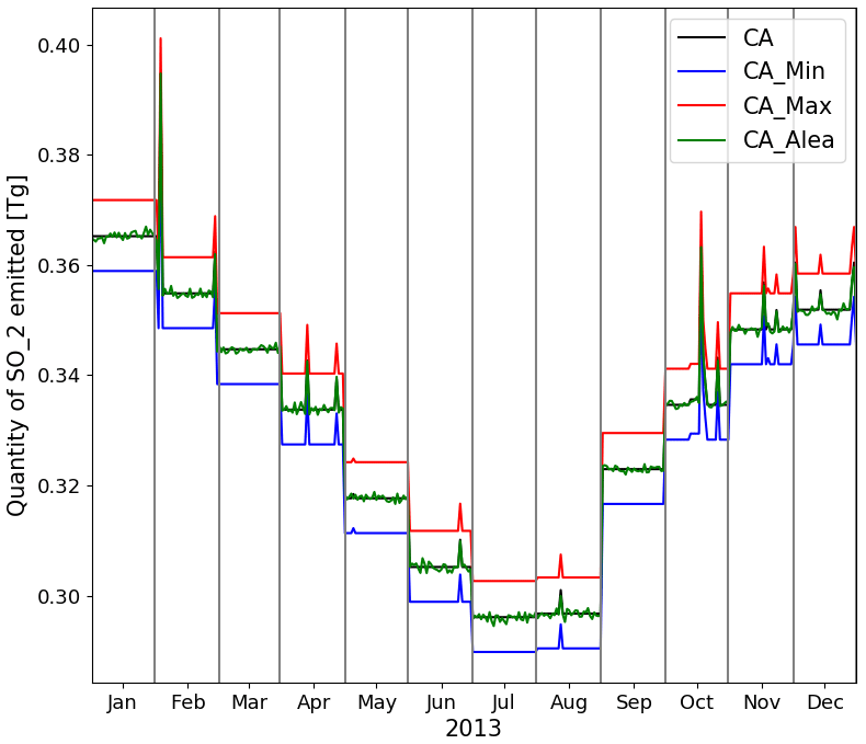
Figure 13Temporal evolution of 2013 SO2 emissions, corresponding to CA (black), CA_MIN (blue), CA_MAX (red) and CA_RAND (green) simulations.
Figure 13 presents the 2013 temporal evolution of SO2 total emission for each simulation. As in Fig. 1, we note the annual variation due to anthropogenic emissions, representing a common basis of around 70 Tg S yr−1 for all simulations, as well as the daily variation due to eruptions, which is shown by the large peaks and representing a value of 0.10 Tg S in 2013. Therefore, the differences are only due to passive degassing SO2 emissions. In the CA simulation, the annual total passive degassing emission is 11.74 Tg S. In the CA_MIN, CA_MAX and CA_RAND experiments, it is 10.60, 12.95 and 11.75 Tg S, respectively. Thus, there is a relative difference of 10.6 % with respect to the annual mean volcanic emissions for CA_MIN simulation but a difference of 1.4 % when considering all sulfur emissions. Similarly, volcanic emissions in CA_MAX and CA_RAND simulations are 9.3 % and 0.1 % higher than in CA, which represents a difference of 1.5 % and <0.01 %, respectively, with respect to the total sulfur emissions.
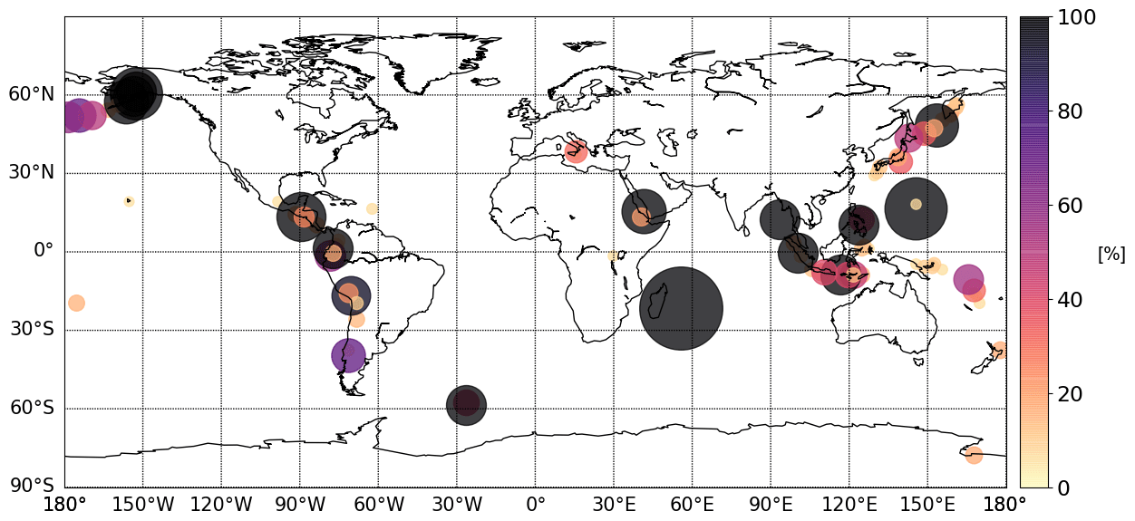
Figure 14Map of ratio of SO2 emissions (in percent) in Carn et al. (2017). The size of the circles is proportional to the value of the ratio, which is also represented by the color.
We expect a greater sensitivity to the annual emission uncertainty at volcanoes where the proportion of the annual uncertainty with respect to the annual mean emission is close to 100 %. Figure 14 represents the percentage of uncertainty on the annual measurement of volcanic emission per volcano in Carn et al. (2017). The darker and bigger the circle is, the more important is the uncertainty compared to the mean emission.
8.2 Sensitivity study on the global budget in MOCAGE
As in Table 5 for CA, Table 6 presents the annual mean global sulfur budget for the CA_MIN, CA_MAX and CA_RAND simulations. Even if the total sulfur species burdens are similar in all simulations, with the SO2 burden around 30 Tg S and the sulfate burden between 0.69–0.72 Tg S, the contribution of the volcanic emissions to the total budget varies. In the CA experiment, the volcanic contribution to the sulfate aerosol burden is 25.40 %, but it ranges from 23.73 % in the CA_MIN experiment to 27.15 % in the CA_MAX experiment. This implies a variation in the efficiency of the model MOCAGE in producing sulfate aerosols from volcanic SO2 emissions. The greatest efficiency score is 1.78 for the CA_MIN simulation, meaning that smaller amounts of SO2 emitted can form sulfate more efficiently. This illustrates the nonlinear relationship between the volcanic SO2 emission and the sulfur budget.
Table 6As in Table 5 but for CA_MIN, CA_MAX and CA_RAND simulations.
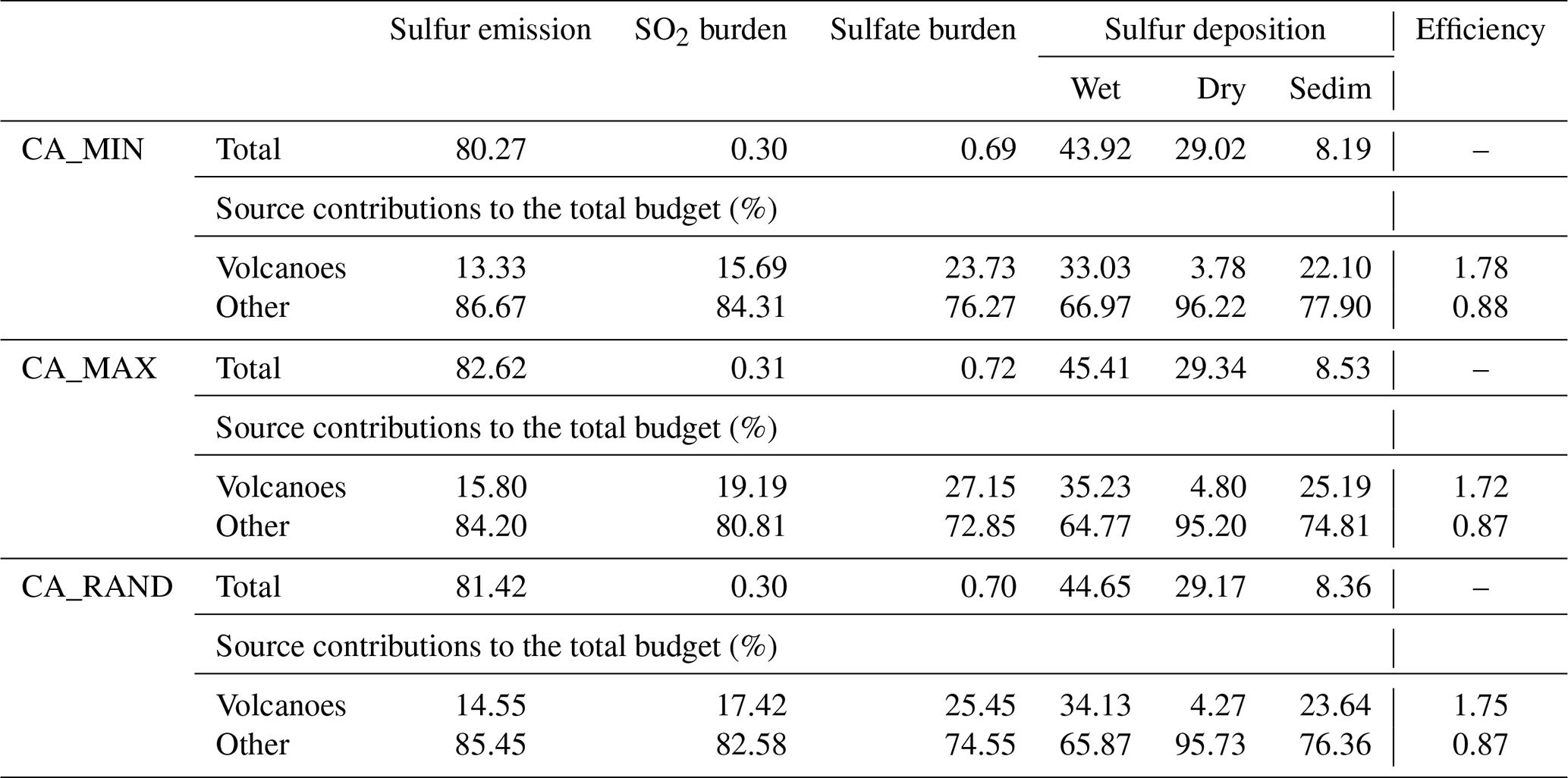
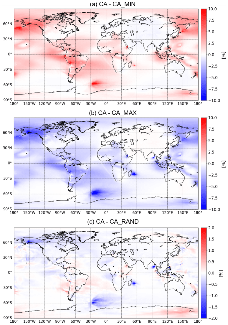
Figure 15The 2013 annual mean difference in SO2 tropospheric column volcanic contribution between CA and (a) CA_MIN, (b) CA_MAX and (c) CA_RAND simulations (in percent).
Figure 15 illustrates the spatial difference in volcanic SO2 contribution between CA and CA_MIN, CA_MAX and CA_RAND. The differences with CA_MIN or CA_MAX (Fig. 15a and b) are similar but of the opposite sign. As expected, differences are located in the vicinity of volcanic point sources but especially near volcanoes with a high ratio (see Fig. 14).
The contribution of volcanic SO2 to the SO2 burden is larger (less important, respectively) in the CA_MAX simulation, with 19.19 % (the CA_MIN simulation, respectively, with 15.69 %), than in the CA simulation, with 17.40 %. The difference between CA and CA_RAND is weaker. Daily variations in SO2 emissions of volcanoes (CA_RAND) do not significantly change the annual mean contribution of the volcanic SO2 tropospheric column. The same conclusions are shown in Fig. S6 for the sulfate tropospheric column.
The differences between the simulations are mostly in the deposition fluxes. Regardless of the sensitivity simulation, the dry sulfur deposition is higher than in the CA simulation. The sulfur wet deposition is 43.90 Tg in the CA simulation but 43.92, 44.65 and 45.41 Tg in the CA_MIN, CA_ALEA and CA_MAX simulations, respectively. It represents a contribution of 33.00 % for CA and 33.03 %, 34.13 % and 35.25 % for CA_MIN, CA_MAX and CA_RAND, respectively. On the contrary, regardless of the sensitivity simulation, the sulfur dry deposition is lower than in the CA simulation. In the CA simulation, the dry deposition is 29.34 Tg (representing a volcanic contribution of 4.80 %), but the dry deposition is 29.34 (4.80 %), 29.17 (4.27 %) and 29.02 Tg (3.78 %) in CA_MAX, CA_ALEA and CA_MIN simulations, respectively. Sedimentation (only due to aerosols) behaves in the expected way; the more volcanic emissions there are, the more sulfur is deposited by sedimentation. The variations in deposition are, thus, due to variations in the deposition of sulfur gases and, more particularly, of SO2. To conclude, sulfur deposition does not react linearly to both the quantities of volcanic SO2 emitted (with respect to CA_MIN and CA_MAX simulations) or to the temporal variability in these emissions (with respect to CA_RAND).
Finally, in the CA_MAX experiment, with the highest estimation of volcanic emissions, we find, as expected, a higher sulfur burden and higher sulfur deposition quantities. However, the CA_MIN simulation assumes the lowest estimate of volcanic SO2 emissions and gives only a slightly lower total sulfur deposition (81.13 compared to 81.60 Tg S in CA) but with a different partition. Even when applying a daily variation, with nearly the same total annual quantity of volcanic SO2 emitted (the CA_RAND simulation), we notice slight changes in the MOCAGE sulfur budget.
In this paper, the aim was to study the contribution of volcanic sulfur emissions on the tropospheric composition and on sulfur species surface concentration and deposition at the global scale. Previously, the volcanic emissions inventory implemented in MOCAGE was from Andres and Kasgnoc (1998), but it has become obsolete. Therefore, a new volcanic SO2 emission inventory, based on Carn et al. (2016, 2017), is implemented in MOCAGE. Thanks to satellite technologies, used to compile this inventory, it includes more volcanoes and gathers both eruptive emissions and passive degassing at a fine time resolution compared to previous inventories. Eruptions are provided as daily total amounts and passive degassing as annual averages with associated annual uncertainties. The inventory also provides information on the plume altitudes. A configuration to inject volcanic emission with an umbrella vertical profile was implemented in the model.
The choice was made to consider the year 2013, when quantities of volcanic SO2 from eruptions are the lowest in the new inventory and negligible in the yearly average. Thereby, the study is focused on passive degassing emissions. A total of two simulations are used to assess the new version of MOCAGE using the Carn et al. (2016, 2017) emissions (CARNALTI) and the associated emission heights with respect to the previous implementation based on Andres and Kasgnoc (1998, REF).
The comparison of the MOCAGE simulations against OMI SO2 total column and MODIS AOD shows that the statistical scores of the model were improved in the CARNALTI simulation compared to REF, especially at the local scale near the volcanoes. The global concentration of SO2 in the MOCAGE simulation is increased with the new inventory. This largely reduces the bias against OMI measurements and increases the correlation with the instrument. Compared to MODIS AOD, the underestimation in aerosol content in the tropics is also reduced. Hence, constraining volcanic emission sources well in chemistry transport models (CTMs) is necessary in order to better represent the tropospheric composition. The comparison to the MODIS AOD provides a method for validating the model results that is independent of the OMI data, which we used for validation but was also used to help estimate the Carn et al. (2016, 2017) emissions.
We showed that considering more volcanoes (both passive degassing and eruptive types) and using a configuration to inject volcanic emissions aloft allows MOCAGE to increase the sulfur species concentrations in CARNALTI compared to REF. At the surface, sulfur species concentrations and depositions were also increased, especially in the vicinity of the volcanoes, affecting air quality in these areas.
Using this new volcanic emissions inventory, we calculated the model sulfur budget in the troposphere. It shows that, even if volcanic emissions represent only 15 % of the total sulfur emissions, the contribution of volcanic SO2 emissions to the sulfur tropospheric burden is nonlinear. Indeed, volcanic sulfate burden is around 25 %, pointing out that the volcanoes' contribution to the sulfur budget is greater than from other sources. Similarly, sulfur deposition due to volcanic emissions contributes unequally to the total sulfur deposition, depending on the nature of deposition; e.g., volcanic sulfate aerosols sedimentation represents the smallest proportion of the total volcanic sulfur deposition (about 11 %) but contributes significantly to the total sulfur sedimentation from all types of SO2 sources (about 24 %).
Moreover, the sensitivity study shows that by increasing, decreasing or including temporal variations in volcanic emission fluxes, the global sulfur budget changes nonlinearly. As an example, despite a reduction in the amount of volcanic SO2 emitted in CA_MIN, the distribution in sulfur deposition varies, causing the decrease in wet deposition but the increase in dry deposition and sedimentation compared to CARNALTI.
These results show that the Carn et al. (2016, 2017) inventory brings an improvement in volcanic SO2 emissions at the global scale. However, there are still remaining uncertainties. Even if recent important progress was made in SO2 remote sensing, there are various uncertainties in SO2 retrievals from satellites of emission mass and height (for eruptions; e.g., vertical sensitivity of the instruments, limits of detection, assumptions in the retrieval algorithm, spatial coverage and data gaps due to clouds) and in the methods used to derive the volcanic emissions from these retrievals. With the constant improvements of space-borne instruments and of methods, more and more accurate volcanic SO2 inventories will be produced in the coming years. For example, the TROPOspheric Monitoring Instrument (TROPOMI), with its high spatial resolution and higher-quality SO2 data set, could provide improved emission inventories (Theys et al., 2019; Fioletov et al., 2020) and could also be used to validate models in similar studies to this one but in a more recent year (2018 and later). Further gains could also be made by increasing the temporal coverage of the satellite observations, which would enable more frequent updating of the emission inventories associated with transient volcanic eruptions. However, this would either require more satellites to be launched into the low Earth orbit or another geostationary satellite.
In this study, we focused on one particular year. By choosing the 2013 year, we mainly study the impact of passive degassing emissions. However, additional studies considering a year in which volcanic eruptions were larger and more frequent would be complementary; e.g., in 2014, 5.35 Tg of eruptive emissions are referenced, which is almost 30 times more than in 2013. It would be interesting to compare and analyze the specific impact of eruptive emissions on the tropospheric sulfur budget. However, the comparison of the tropospheric sulfur budget between different years cannot only be affected by the differences in volcanic sulfur emissions. Indeed, sulfur dioxide is a soluble species, and the meteorological parameters can also impact the tropospheric sulfur budget; e.g., differences in precipitation can lead to changes in the wet deposition fluxes. Thus, meteorological parameters should be taken into account when analyzing the interannual differences.
Finally, it could also be interesting to not only compare 2 years of the Carn et al. (2016, 2017) but to fully study the interannual variability in volcanic sulfur emissions over a longer period. Since the data are fully available over a decade (2005–2015), this type of study would be possible.
The new volcanic SO2 inventory implemented is available for eruptive emissions from the GES DISC archive (https://doi.org/10.5067/MEASURES/SO2/DATA405, Carn, 2021). Passive degassing emissions can be found in Carn et al. (2017, https://doi.org/10.1038/srep44095) and their accompanying supplementary material (https://doi.org/10.1038/srep44095). Concerning the data used for the validation, OMI SO2 total column data can be found in the NASA database GES DISC (Li et al., 2020; https://doi.org/10.5067/Aura/OMI/DATA2022). The previous volcanic SO2 inventory is available upon request from the corresponding author.
The supplement related to this article is available online at: https://doi.org/10.5194/acp-21-11379-2021-supplement.
CL, JG and VM designed the study and the model experiments. Simulations were carried out by CL, with help from JG and MC. The paper was written by CL and reviewed, commented on and edited by VM, JG, NT, PDH and PS. All authors approved the article.
The authors declare that they have no conflict of interest.
Publisher's note: Copernicus Publications remains neutral with regard to jurisdictional claims in published maps and institutional affiliations.
We would like to acknowledge the MODIS mission team and scientists for the production of the data used in this study. The authors thank Météo-France for hosting Claire Lamotte's doctoral research at the Centre National de Recherches Météorologiques.
The doctoral research contract of Claire Lamotte has been supported by the Université Paul Sabatier Toulouse III.
This paper was edited by Jianzhong Ma and reviewed by two anonymous referees.
Aas, W., Mortier, A., Bowersox, V., Cherian, R., Faluvegi, G., Fagerli, H., Hand, J., Klimont, Z., Galy-Lacaux, C., Lehmann, C. M. B., Lund Myhre, C., Myhre, G., Olivié, D., Sato, K., Quaas, J., Rao, P. S. P., Schulz, M., Shindell, D., Skeie, R. B., Stein, A., Takemura, T., Tsyro, S., Vet, R., and Xu, X.: Global and regional trends of atmospheric sulfur, Sci. Rep., 9, 953, https://doi.org/10.1038/s41598-018-37304-0, 2019. a
Adams, P. J., Seinfeld, J. H., Koch, D., Mickley, L., and Jacob, D.: General circulation model assessment of direct radiative forcing by the sulfate-nitrate-ammonium-water inorganic aerosol system, J. Geophys. Res., 106, 1097–1111, https://doi.org/10.1029/2000JD900512, 2001. a
Andreae, M. O.: The Biogeochemical Cycling of Sulfur and Nitrogen in the Remote Atmosphere, Mathematical and Physical Sciences C, 159, chap. 1, 5–25, D. Reidel Publishing Company, Dordrecht, 1985. a
Andres, R. and Kasgnoc, A.: A time-averaged inventory of subaerial volcanic sulful emissions, J. Geophys. Res., 103, 25251–25261, https://doi.org/10.1029/98JD02091, 1998. a, b, c, d, e, f, g, h, i, j, k, l, m, n, o, p, q, r, s, t, u, v, w, x, y, z, aa, ab, ac
Barré, J., Peuch, V.-H., Attié, J.-L., El Amraoui, L., Lahoz, W. A., Josse, B., Claeyman, M., and Nédélec, P.: Stratosphere-troposphere ozone exchange from high resolution MLS ozone analyses, Atmos. Chem. Phys., 12, 6129–6144, https://doi.org/10.5194/acp-12-6129-2012, 2012. a
Bechtold, P., Bazile, E., Guichard, F., Mascart, P., and Richard, E.: A mass-flux convection scheme for regional and global models, Q. J. Roy. Meteor. Soc., 127, 869–886, https://doi.org/10.1002/qj.49712757309, 2001. a
Berresheim, H. and Jaeschke, W.: The contribution of volcanoes to the global atmospheric sulfur budget, J. Geophys. Res., 88, 3732–3740, 1983. a
Boichu, M., Chiapello, I., Brogniez, C., Péré, J.-C., Thieuleux, F., Torres, B., Blarel, L., Mortier, A., Podvin, T., Goloub, P., Söhne, N., Clarisse, L., Bauduin, S., Hendrick, F., Theys, N., Van Roozendael, M., and Tanré, D.: Current challenges in modelling far-range air pollution induced by the 2014–2015 Bárðarbunga fissure eruption (Iceland), Atmos. Chem. Phys., 16, 10831–10845, https://doi.org/10.5194/acp-16-10831-2016, 2016. a
Boichu, M., Favez, O., Riffault, V., Petit, J.-E., Zhang, Y., Brogniez, C., Sciare, J., Chiapello, I., Clarisse, L., Zhang, S., Pujol-Söhne, N., Tison, E., Delbarre, H., and Goloub, P.: Large-scale particulate air pollution and chemical fingerprint of volcanic sulfate aerosols from the 2014–2015 Holuhraun flood lava eruption of Bárðarbunga volcano (Iceland), Atmos. Chem. Phys., 19, 14253–14287, https://doi.org/10.5194/acp-19-14253-2019, 2019. a
Carboni, E., Grainger, R., Walker, J., Dudhia, A., and Siddans, R.: A new scheme for sulphur dioxide retrieval from IASI measurements: application to the Eyjafjallajökull eruption of April and May 2010, Atmos. Chem. Phys., 12, 11417–11434, https://doi.org/10.5194/acp-12-11417-2012, 2012. a
Carn, S.: Multi-Satellite Volcanic Sulfur Dioxide L4 Long-Term Global Database V3, Goddard Earth Science Data and Information Services Center (GES DISC) [data set], Greenbelt, MD, USA, https://doi.org/10.5067/MEASURES/SO2/DATA405, 2021. a, b, c, d
Carn, S., Krotkov, N., Yang, K., and Krueger, A.: Measuring global volcanic degassing with the Ozone Monitoring Instrument (OMI), Geol. Soc. Sp., 380, 229–257, https://doi.org/10.1144/SP380.12, 2013. a
Carn, S., Clarisse, L., and Prata, A.: Multi-decadal satellite measurement of global volcanic degassing, J. Volcanol. Geoth. Res., 311, 99–134, https://doi.org/10.1016/j.jvolgeores.2016.01.002, 2016. a, b, c, d, e, f, g, h, i, j, k, l, m, n, o, p, q, r, s, t, u, v, w, x, y, z, aa, ab, ac, ad, ae, af, ag, ah, ai, aj, ak, al, am, an, ao, ap
Carn, S., Fioletov, V., McLinden, C., Li, C., and Krotkov, N.: A decade of global volcanic SO2 emissions measured from space, Sci. Rep., 7, 44095, https://doi.org/10.1038/srep44095, 2017. a, b, c, d, e, f, g, h, i, j, k, l, m, n, o, p, q, r, s, t, u, v, w, x, y, z, aa, ab, ac, ad, ae, af, ag, ah, ai, aj, ak, al, am, an, ao, ap, aq, ar, as
Castro, L. M., Pio, C. A., Harrison, R. M., and Smith, D. J. T.: Carbonaceous areosol in urban and rural European atmopsheres: estimation of secondary organic carbon concentrations, Atmos. Environ., 33, 2771–2781, https://doi.org/10.1016/S1352-2310(98)00331-8, 1999. a
Chestnut, L.: Human Health Benefits From Sulfate Reductions Under Title IV of the 1990 Clean Air Act Amendments, Final Report, Tech. Rep., US EPA, Office of Atmospheric Programs, Acid Rain Division, Washington DC, 1995. a
Chin, M. and Jacob, D.: Anthropogenic and natural contributions to tropospheric sulfate: A global model analysis, J. Geophys. Res., 101, 18691–18699, https://doi.org/10.1029/96JD01222, 1996. a, b, c, d
Chin, M., Rood, R. B., Lin, S.-J., Muller, J.-F., and Thompson, A. M.: Atmospheric sulfur cycle simulated in the global model GOCART: Model description and global properties, J. Geophys. Res., 105, 24671–24687, https://doi.org/10.1029/2000JD900384, 2000. a
Clarisse, L., Coheur, P.-F., Theys, N., Hurtmans, D., and Clerbaux, C.: The 2011 Nabro eruption, a SO2 plume height analysis using IASI measurements, Atmos. Chem. Phys., 14, 3095–3111, https://doi.org/10.5194/acp-14-3095-2014, 2014. a
Colette, A., Favez, O., Meleux, F., Chiappini, L., Haeffelin, M., Y., M., Malherbe, L., Papin, A., Bessagnet, B., Menut, L., Leoz, E., and Rouïl, L.: Assessing in nearl real time the impact of April 2010 Eyjafjallajökull ash plume on air quality, Atmos. Environ., 45, 1217–1221, https://doi.org/10.1016/j.atmosenv.2010.09.064, 2010. a
Courtier, P., Freydier, C., Geleyn, J.-F., Rabier, F., and Rochas, M.: The ARPEGE project at Météo-France, in: ECMWF Workshop, Reading, England, 9–13 September 1991, Abstract no. 8798, 1991. a
Cussac, M., Marécal, V., Thouret, V., Josse, B., and Sauvage, B.: The impact of biomass burning on upper tropospheric carbon monoxide: a study using MOCAGE global model and IAGOS airborne data, Atmos. Chem. Phys., 20, 9393–9417, https://doi.org/10.5194/acp-20-9393-2020, 2020. a
Dai, T., Schutgens, N., Goto, D., Shi, G., and Nakajima, T.: Improvement of aerosol optical properties modeling over Eastern Asia with MODIS AOD assimilation in a global non-hydrostatic icosahedral aerosol transport model, Environ. Pollut., 195, 319–329, https://doi.org/10.1016/j.envpol.2014.06.021, 2014. a
Descheemaecker, M., Plu, M., Marécal, V., Claeyman, M., Olivier, F., Aoun, Y., Blanc, P., Wald, L., Guth, J., Sič, B., Vidot, J., Piacentini, A., and Josse, B.: Monitoring aerosols over Europe: an assessment of the potential benefit of assimilating the VIS04 measurements from the future MTG/FCI geostationary imager, Atmos. Meas. Tech., 12, 1251–1275, https://doi.org/10.5194/amt-12-1251-2019, 2019. a, b
Diehl, T., Heil, A., Chin, M., Pan, X., Streets, D., Schultz, M., and Kinne, S.: Anthropogenic, biomass burning, and volcanic emissions of black carbon, organic carbon, and SO2 from 1980 to 2010 for hindcast model experiments, Atmos. Chem. Phys. Discuss., 12, 24895–24954, https://doi.org/10.5194/acpd-12-24895-2012, 2012. a
El Amraoui, L., Attié, J.-L., Semane, N., Claeyman, M., Peuch, V.-H., Warner, J., Ricaud, P., Cammas, J.-P., Piacentini, A., Josse, B., Cariolle, D., Massart, S., and Bencherif, H.: Midlatitude stratosphere – troposphere exchange as diagnosed by MLS O3 and MOPITT CO assimilated fields, Atmos. Chem. Phys., 10, 2175–2194, https://doi.org/10.5194/acp-10-2175-2010, 2010. a
Emmons, L. K., Walters, S., Hess, P. G., Lamarque, J.-F., Pfister, G. G., Fillmore, D., Granier, C., Guenther, A., Kinnison, D., Laepple, T., Orlando, J., Tie, X., Tyndall, G., Wiedinmyer, C., Baughcum, S. L., and Kloster, S.: Description and evaluation of the Model for Ozone and Related chemical Tracers, version 4 (MOZART-4), Geosci. Model Dev., 3, 43–67, https://doi.org/10.5194/gmd-3-43-2010, 2010. a
Feichter, J., Kjellström, E., Rodhe, H., Dentener, F., Lelieveldi, J., and Roelofs, G.-J.: Simulation of the tropospheric sulfur cycle in a global climate model, Atmos. Environ., 30, 1693–1707, https://doi.org/10.1016/1352-2310(95)00394-0, 1996. a
Feinberg, A., Sukhodolov, T., Luo, B.-P., Rozanov, E., Winkel, L. H. E., Peter, T., and Stenke, A.: Improved tropospheric and stratospheric sulfur cycle in the aerosol–chemistry–climate model SOCOL-AERv2, Geosci. Model Dev., 12, 3863–3887, https://doi.org/10.5194/gmd-12-3863-2019, 2019. a, b, c, d, e, f
Fioletov, V. E., McLinden, C. A., Krotkov, N., Yang, K., Loyola, D. G., Valks, P., Theys, N., Van Roozendael, M., Nowlan, C. R., Chance, K., Liu, X., Lee, C., and Martin, R. V.: Application of OMI, SCIAMACHY, and GOME-2 satellite SO2 retrievals for detection of large emission sources, J. Geophys. Res.-Atmos., 118, 11399–11418, https://doi.org/10.1002/jgrd.50826, 2013. a, b
Fioletov, V. E., McLinden, C. A., Krotkov, N., Li, C., Joiner, J., Theys, N., Carn, S., and Moran, M. D.: A global catalogue of large SO2 sources and emissions derived from the Ozone Monitoring Instrument, Atmos. Chem. Phys., 16, 11497–11519, https://doi.org/10.5194/acp-16-11497-2016, 2016. a
Fioletov, V., McLinden, C. A., Griffin, D., Theys, N., Loyola, D. G., Hedelt, P., Krotkov, N. A., and Li, C.: Anthropogenic and volcanic point source SO2 emissions derived from TROPOMI on board Sentinel-5 Precursor: first results, Atmos. Chem. Phys., 20, 5591–5607, https://doi.org/10.5194/acp-20-5591-2020, 2020. a
Fountoukis, C. and Nenes, A.: ISORROPIA II: a computationally efficient thermodynamic equilibrium model for aerosols, Atmos. Chem. Phys., 7, 4639–4659, https://doi.org/10.5194/acp-7-4639-2007, 2007. a
Freitas, S. R., Longo, K. M., Alonso, M. F., Pirre, M., Marecal, V., Grell, G., Stockler, R., Mello, R. F., and Sánchez Gácita, M.: PREP-CHEM-SRC – 1.0: a preprocessor of trace gas and aerosol emission fields for regional and global atmospheric chemistry models, Geosci. Model Dev., 4, 419–433, https://doi.org/10.5194/gmd-4-419-2011, 2011. a
Gasso, S.: Satellite observations of the impact of weak volcanic activity on marine clouds, J. Geophys. Res., 113, D14S19, https://doi.org/10.1029/2007JD009106, 2008. a
Ge, C., Wang, J., Carn, S., Yang, K., Ginoux, P., and Krotkov, N.: Satellite-based global volcanic SO2 emissions and sulfate direct radiative forcing during 2005–2012, J. Geophys. Res., 121, 1–19, https://doi.org/10.1002/2015JD023134, 2016. a, b
Gondwe, M., Krol, M., Gieskes, W., Klaasen, W., and de Baar, H.: The contribution of ocean-leaving DMS to the global atmospheric burdens of DMS, MSA, SO2 and NSS , Global Biogeochem. Cy., 17, 1056, https://doi.org/10.1029/2002GB001937, 2003a. a
Gondwe, M., Krol, M., Gieskes, W., Klaasen, W., and de Baar, H.: Correcttion to “The contribution of ocean-leaving DMS to the global atmospheric burdens of DMS, MSA, SO2 and NSS ”, Global Biogeochem. Cy., 17, 1106, https://doi.org/10.1029/2003GB002153, 2003b. a
Graf, H.-F., Feichter, J., and Langmann, B.: Volcanic sulfur emissions: Estimates of source strength and its contribution to the global sulfate distribution, J. Geophys. Res., 102, 10727–10728, https://doi.org/10.1029/96JD03265, 1997. a, b, c, d, e, f, g, h, i, j
Graf, H.-F., Langmann, B., and Feichter, J.: The contribution of Earth degassing to the atmospheric sulfur budget, Chem. Geol., 147, 131–145, https://doi.org/10.1016/S0009-2541(97)00177-0, 1998. a
Gunson, J. R., Spall, S. A., Anderson, T. R., Jones, A., Totterdell, I. J., and Woodage, M. J.: Climate sensitivity to ocean dimethylsulphide emissions, Geophys. Res. Lett., 33, L07701, https://doi.org/10.1029/2005GL024982, 2006. a
Guth, J.: Modélisation des aérosols à l'aide du modèle de chimie-transport MOCAGE : application à la qualité de l'air dans le bassin méditerranéen, Ph.D. thesis, Université Toulouse III Paul Sabatier, Toulouse, 2015. a, b
Guth, J., Josse, B., Marécal, V., Joly, M., and Hamer, P.: First implementation of secondary inorganic aerosols in the MOCAGE version R2.15.0 chemistry transport model, Geosci. Model Dev., 9, 137–160, https://doi.org/10.5194/gmd-9-137-2016, 2016. a, b, c, d, e
Guth, J., Marécal, V., Josse, B., Arteta, J., and Hamer, P.: Primary aerosol and secondary inorganic aerosol budget over the Mediterranean Basin during 2012 and 2013, Atmos. Chem. Phys., 18, 4911–4934, https://doi.org/10.5194/acp-18-4911-2018, 2018. a
Halmer, M., Schmincke, H.-U., and Graf, H.-F.: The annual volcanic gas input into the atmosphere, in particular into the stratosphere: a global data set for the past 100 years, J. Volcanol. Geoth. Res., 115, 511–528, https://doi.org/10.1016/S0377-0273(01)00318-3, 2002. a
He, H., Li, C., Loughner, C. P., Li, Z., Krotkov, N. A., Yang, K., Wang, L., Zheng, Y., Bao, X., Zhao, G., and Dickerson, R. R.: SO2 over central China: Measurements, numerical simulations and the tropospheric sulfur budget, J. Geophys. Res., 117, D00K37, https://doi.org/10.1029/2011JD016473, 2012. a, b
Josse, B., Simon, P., and Peuch, V.: Radon global simulations with the multiscale chemistry and transport model MOCAGE, Tellus B, 56, 339–356, https://doi.org/10.3402/tellusb.v56i4.16448, 2004. a, b
Kaiser, J. W., Heil, A., Andreae, M. O., Benedetti, A., Chubarova, N., Jones, L., Morcrette, J.-J., Razinger, M., Schultz, M. G., Suttie, M., and van der Werf, G. R.: Biomass burning emissions estimated with a global fire assimilation system based on observed fire radiative power, Biogeosciences, 9, 527–554, https://doi.org/10.5194/bg-9-527-2012, 2012. a
Kettle, A., Andreae, M. O., Amouroux, D., Andreae, T. W., Bates, T. S., Berresheim, H., Bingemer, H., Boniforti, R., Curran, M., DiTullio, G. R., Helas, G., Jones, G. B., Kiene, R. P., Leck, C., Levasseur, M., Malin, G., Maspero, M., Matrai, P., McTaggart, A. R., Mihalopoulos, N., Nguyen, B. C., Novo, A., Putaud, J. P., Rapsomanikis, S., Roberts, G., Schebeske, G., Sharma, S., Simó, R., Staubes, R., Turner, S., and Uher, G.: A global database of sea surface dimethylsulfide (DMS) measurements and a procedure to predict sea surface DMS as a function of latitude, longitude, and month, Global Biogeochem. Cy., 13, 399–444, https://doi.org/10.1029/1999GB900004, 1999. a
Koren, I., Remer, L. A., Kaufman, Y. J., Rudich, Y., and Martins, J. V.: On the twilight zone between clouds and aerosols, Geophys. Res. Lett., 34, L08805, https://doi.org/10.1029/2007GL029253, 2007. a
Kremser, S., Thomason, L. W., von Hobe, M., Hermann, M., Deshler, T., Timmreck, C., Toohey, M., Stenke, A., Schwarz, J. P., Weigel, R., Fueglistaler, S., Prata, F. J., Vernier, J.-P., Schlager, H., Barnes, J. E., Antuña-Marrero, J.-C., Fairlie, D., Palm, M., Mahieu, E., Notholt, J., Rex, M., Bingen, C., Vanhellemont, F., Bourassa, A., Plane, J. M. C., Klocke, D., Carn, S. A., Clarisse, L., Trickl, T., Neely, R., James, A. D., Rieger, L., Wilson, J. C., and Meland, B.: Stratospheric aerosol–Observations, processes, and impact on climate, Rev. Geophys., 54, 278–335, https://doi.org/10.1002/2015RG000511, 2016. a
Krotkov, N. A., McLinden, C. A., Li, C., Lamsal, L. N., Celarier, E. A., Marchenko, S. V., Swartz, W. H., Bucsela, E. J., Joiner, J., Duncan, B. N., Boersma, K. F., Veefkind, J. P., Levelt, P. F., Fioletov, V. E., Dickerson, R. R., He, H., Lu, Z., and Streets, D. G.: Aura OMI observations of regional SO2 and NO2 pollution changes from 2005 to 2015, Atmos. Chem. Phys., 16, 4605–4629, https://doi.org/10.5194/acp-16-4605-2016, 2016. a
Krueger, A., Walter, L., Bhartia, P., Schnetzler, C., Krotkov, N., Sprod, I., and Bluth, G.: Volcanic sulfur dioxide measurements from the total ozone mapping spectrometer instruments, J. Geophys. Res., 100, 14057–14076, https://doi.org/10.1029/95JD01222, 1995. a, b
Köpke, P., Hess, M., Schult, I., and Shettle, E.: Global Aerosol Data Set, Max-Planck-Institut für Meteorologie, Hambourg, Germany, http://hdl.handle.net/10068/256361 (last access: July 2018), 1997. a
Lacressonnière, G., Peuch, V.-H., Vautard, R. Arteta, J., Déqué, M. an Joly, M., Josse, B., Marécal, V., and Saint-Martin, D.: European air quality in the 2030s and 2050s: Impacts of global and regional emission trends and of climate change, Atmos. Environ., 92, 348–358, https://doi.org/10.1016/j.atmosenv.2014.04.033, 2014. a
Lacressonnière, G., Foret, G., Beekmann, M., Siour, G., Engardt, M., Gauss, M., Watson, L., Andersson, C., Colette, A., Josse, B., Marécal, V., Nyiri, A., and Vautard, R.: Impacts of regional climate change on air quality projections and associated uncertainties, Climatic Change, 136, 309–324, https://doi.org/10.1007/s10584-016-1619-z, 2016. a
Lacressonnière, G., Watson, L., Gauss, M., Engardt, M., Andersson, C., Beekmann, M., Colette, A., Foret, G., Josse, B., Marécal, V., Nyiri, A., Siour, G., Sobolowski, S., and Vautard, R.: Particulate matter air pollution in Europe in a +2 ∘C warming world, Atmos. Environ., 154, 129–140, https://doi.org/10.1016/j.atmosenv.2017.01.037, 2017. a
Lamarque, J.-F., Bond, T. C., Eyring, V., Granier, C., Heil, A., Klimont, Z., Lee, D., Liousse, C., Mieville, A., Owen, B., Schultz, M. G., Shindell, D., Smith, S. J., Stehfest, E., Van Aardenne, J., Cooper, O. R., Kainuma, M., Mahowald, N., McConnell, J. R., Naik, V., Riahi, K., and van Vuuren, D. P.: Historical (1850–2000) gridded anthropogenic and biomass burning emissions of reactive gases and aerosols: methodology and application, Atmos. Chem. Phys., 10, 7017–7039, https://doi.org/10.5194/acp-10-7017-2010, 2010. a, b, c
Lamarque, J.-F., Emmons, L. K., Hess, P. G., Kinnison, D. E., Tilmes, S., Vitt, F., Heald, C. L., Holland, E. A., Lauritzen, P. H., Neu, J., Orlando, J. J., Rasch, P. J., and Tyndall, G. K.: CAM-chem: description and evaluation of interactive atmospheric chemistry in the Community Earth System Model, Geosci. Model Dev., 5, 369–411, https://doi.org/10.5194/gmd-5-369-2012, 2012. a
Lamarque, J.-F., Shindell, D. T., Josse, B., Young, P. J., Cionni, I., Eyring, V., Bergmann, D., Cameron-Smith, P., Collins, W. J., Doherty, R., Dalsoren, S., Faluvegi, G., Folberth, G., Ghan, S. J., Horowitz, L. W., Lee, Y. H., MacKenzie, I. A., Nagashima, T., Naik, V., Plummer, D., Righi, M., Rumbold, S. T., Schulz, M., Skeie, R. B., Stevenson, D. S., Strode, S., Sudo, K., Szopa, S., Voulgarakis, A., and Zeng, G.: The Atmospheric Chemistry and Climate Model Intercomparison Project (ACCMIP): overview and description of models, simulations and climate diagnostics, Geosci. Model Dev., 6, 179–206, https://doi.org/10.5194/gmd-6-179-2013, 2013. a
Lefèvre, F., Brasseur, P., Folkins, I., Smith, A. K., and Simon, P.: Chemistry of the 1991–1992 stratospheric winter: Three-dimensional simulations, J. Geophys. Res., 99, 8183–8195, https://doi.org/10.1029/93JD03476, 1994. a
Li, C., Joiner, J., Krotkov, N., and Bhartia, P.: A fast and sensitive new satellite SO2 retrieval algorithm based on principal component analysis: Application to the ozone monitoring instrument, Geophys. Res. Lett., 40, 6314–6318, https://doi.org/10.1002/2013GL058134, 2013. a, b
Li, C., Krotkov, N. A., Leonard, P., and Joiner, J.: OMI/Aura Sulphur Dioxide (SO2) Total Column 1-orbit L2 Swath 13x24 km V003, Greenbelt, MD, USA, Goddard Earth Sciences Data and Information Services Center (GES DISC) [data set], https://doi.org/10.5067/Aura/OMI/DATA2022, 2020. a, b
Liu, X., Penner, J. E., and Herzog, M.: Global modeling of aerosol dynamics: Model description, evaluatio, and interactions between sulfate and nonsulfate aerosols, J. Geophys. Res., 110, D18206, https://doi.org/10.1029/2004JD005674, 2005. a
iu, X., Penner, J. E., Das, B., Bergmann, D., Rodriguez, J. M., Strahan, S., Wang, M., and Feng, Y.: Uncertainties in global aerosol simulations: Assessment using three meteorological data sets, J. Geophys. Res., 112, D11212, https://doi.org/10.1029/2006JD008216, 2007. a
Liu, Z., Liu, Q., Lin, H.-C., Schwartz, C. S., Lee, Y.-H., and Wang, T.: Three-dimensional variational assimilation of MODIS aerosol optical depth: Implementation and application to a dust storm over East Asia, J. Geophys. Res., 116, D23206, https://doi.org/10.1029/2011JD016159, 2011. a
Louis, J.-F.: A parametric model of vertical eddy fluxes in the atmopshere, Bound.-Lay. Meteorol., 17, 187–202, https://doi.org/10.1007/BF00117978, 1979. a
Madronich, S.: Photodissociation in the atmosphere: 1. Actinic flux and the effects of ground reflections and clouds, J. Geophys. Res.-Atmos., 92, 9740–9752, https://doi.org/10.1029/JD092iD08p09740, 1987. a
Martet, M., Peuch, V., Laurent, B., Marticorena, B., and Bergametti, G.: Evaluation of long-range transport and deposition of desert dust with the CTM MOCAGE, Tellus B, 61, 449–463, https://doi.org/10.1111/j.1600-0889.2008.00413.x, 2009. a
Marécal, V., Peuch, V.-H., Andersson, C., Andersson, S., Arteta, J., Beekmann, M., Benedictow, A., Bergström, R., Bessagnet, B., Cansado, A., Chéroux, F., Colette, A., Coman, A., Curier, R. L., Denier van der Gon, H. A. C., Drouin, A., Elbern, H., Emili, E., Engelen, R. J., Eskes, H. J., Foret, G., Friese, E., Gauss, M., Giannaros, C., Guth, J., Joly, M., Jaumouillé, E., Josse, B., Kadygrov, N., Kaiser, J. W., Krajsek, K., Kuenen, J., Kumar, U., Liora, N., Lopez, E., Malherbe, L., Martinez, I., Melas, D., Meleux, F., Menut, L., Moinat, P., Morales, T., Parmentier, J., Piacentini, A., Plu, M., Poupkou, A., Queguiner, S., Robertson, L., Rouïl, L., Schaap, M., Segers, A., Sofiev, M., Tarasson, L., Thomas, M., Timmermans, R., Valdebenito, Á., van Velthoven, P., van Versendaal, R., Vira, J., and Ung, A.: A regional air quality forecasting system over Europe: the MACC-II daily ensemble production, Geosci. Model Dev., 8, 2777–2813, https://doi.org/10.5194/gmd-8-2777-2015, 2015. a
Michou, M., Nabat, P., and Saint-Martin, D.: Development and basic evaluation of a prognostic aerosol scheme (v1) in the CNRM Climate Model CNRM-CM6, Geosci. Model Dev., 8, 501–531, https://doi.org/10.5194/gmd-8-501-2015, 2015. a
Michou, M., Nabat, P., Saint-Martin, D., Bock, J., Decharme, B., Mallet, M., Roehrig, R., Séférian, R., Sénési, S., and Voldoire, A.: Present-Day and Historical Aerosol and Ozone Characteristics in CNRM CMIP6 Simulations, J. Adv. Model. Earth Sy., 12, e2019MS001816, https://doi.org/10.1029/2019MS001816, 2020. a
Moffat, A. and Millan, M.: The application of optical correlation techniques to the remote sensing of SO2 plumes using sky light, Atmos. Environ., 5, 677–690, https://doi.org/10.1016/0004-6981(71)90125-9, 1971. a, b
Nenes, A., Pilinis, C., and Pandis, N.: ISORROPIA: A new thermodynamic equilibrium model for multiphase multicomponent inorganic aerosols, Aquat. Geochem., 4, 123–152, https://doi.org/10.1023/A:1009604003981, 1998. a
Nowlan, C., Liu, X., Chance, K., Cai, Z., Kurosu, T., Lee, C., and Martin, R.: Retrieval of sulfur dioxide from the Global Ozone Monitoring Experiment 2 (GOME-2) using an optimal estimation approach: Algorithm and initial validation, J. Geophys. Res., 116, D18301, https://doi.org/10.1029/2011JD015808, 2011. a
Pham, M., Muller, J., Brasseur, G. P., Granier, C., and Megie, G.: A three-dimensional study of the tropospheric sulfur cycle, J. Geophys. Res., 100, 26061–26092, https://doi.org/10.1029/95JD02095, 1995. a
Price, C., Penner, J., and Prather, M.: NOx from lightning: 1. global distribution based on lightning physics, J. Geophys. Res.-Atmos., 102, 5929–5941, https://doi.org/10.1029/96JD03504, 1997. a, b
Remer, L. A., Kleidman, R. G., Levy, R. C., Kaufman, Y. J., Tanré, D., Mattoo, S., Vanderlei Martins, J. V., Ichoku, C., Koren, I., Yu, H., and Holben, B. N.: Global aerosol climatology from the MODIS satellite sensors, J. Geophys. Res., 113, D14S07, https://doi.org/10.1029/2007JD009661, 2008. a
Richter, A., Wittrock, F., and Burrows, J. P.: SO2 measurements with SCIAMACHY, in: European Space Agency Center for Earth Observation, Atmospheric Science Conference, Frascati, Italy, 8–12 May 2006, Abstract no. 2006ESASP.628E..51R, 2006. a
Rix, M., Valks, P., Hao, N., Loyola, D., Schlager, H., Huntrieser, H., Flemming, J., Koehler, U., Schumann, U., and Inness, A.: Volcanic SO2, BrO and plume height estimations using GOME-2 satellite measurements during the eruption of Eyjafjallajökull in May 2010, J. Geophys. Res., 117, D00U19, https://doi.org/10.1029/2011JD016718, 2012. a
Robock, A.: Volcanic eruptions and climate, Rev. Geophys., 38, 191–219, https://doi.org/10.1029/1998RG000054, 2000. a, b
Robock, A.: Correction to “Volcanic eruptions and climate”, Rev. Geophys., 45, RG3005, https://doi.org/10.1029/2007RG000232, 2007. a
Rouil, L., Honoré, C., Bessagnet, B., Malherbe, L., Meleux, F., Vautard, R., Beekmann, M., Flaud, J.-M., Dufour, A., Martin, D., Peuch, A., Peuch, V.-H., Elichegaray, C., Poisson, N., and Menut, L.: PREV'AIR: an operational forecasting and mapping system for air quality in Europe, B. Am. Meteorol. Soc., 90, 73–84, https://doi.org/10.1175/2008BAMS2390.1, 2009. a
Ruiz-Arias, J. A., Dudhia, J., Gueymard, C. A., and Pozo-Vázquez, D.: Assessment of the Level-3 MODIS daily aerosol optical depth in the context of surface solar radiation and numerical weather modeling, Atmos. Chem. Phys., 13, 675–692, https://doi.org/10.5194/acp-13-675-2013, 2013. a
Savage, N. H., Agnew, P., Davis, L. S., Ordóñez, C., Thorpe, R., Johnson, C. E., O'Connor, F. M., and Dalvi, M.: Air quality modelling using the Met Office Unified Model (AQUM OS24-26): model description and initial evaluation, Geosci. Model Dev., 6, 353–372, https://doi.org/10.5194/gmd-6-353-2013, 2013. a
Schaefer, S. J., Kerr, J. B., Millán, M. M., Realmuto, V. J., Krueger, A. J., Krotkov, N. A., Seftor, C., and Sprod, I. E.: Geophysicists Unite to Validate Volcanic SO2 Measurements, EOS T. Am. Geophys. Un., 78, 217–223, https://doi.org/10.1029/97EO00144, 1997. a
Schenkeveld, V. M. E., Jaross, G., Marchenko, S., Haffner, D., Kleipool, Q. L., Rozemeijer, N. C., Veefkind, J. P., and Levelt, P. F.: In-flight performance of the Ozone Monitoring Instrument, Atmos. Meas. Tech., 10, 1957–1986, https://doi.org/10.5194/amt-10-1957-2017, 2017. a
Schmidt, A., Carslaw, K. S., Mann, G. W., Rap, A., Pringle, K. J., Spracklen, D. V., Wilson, M., and Forster, P. M.: Importance of tropospheric volcanic aerosol for indirect radiative forcing of climate, Atmos. Chem. Phys., 12, 7321–7339, https://doi.org/10.5194/acp-12-7321-2012, 2012. a
Schmidt, A., Leadbetter, S., Theys, N., Carboni, E., Witham, C. S., Stevenson, J. A., Birch, C. E., Thordarson, T., Turnock, S., Barsotti, S., Delaney, L., Feng, W., Grainger, R. G., Hort, M. C., Höskuldsson, A., Ialongo, I., Ilyinskaya, E., Jóhannsson, T., Kenny, P., Mather, T. A., Richards, N. A. D., and Shepherd, J.: Satellite detection, long-range transport, and air quality impacts of volcanic sulfur dioxide from the 2014–2015 flood lava eruption at Bárðarbunga (Iceland), J. Geophys. Res., 120, 9739–9757, https://doi.org/10.1002/2015JD023638, 2015. a
Seftor, C., Hsu, N., Herman, J., Bhartia, P., Torres, O., Rose, W., Schneider, D., and Krotkov, N.: Detection of volcanic ash clouds from Nimbus 7/total ozone mapping spectrometer, J. Geophys. Res., 102, 16749–16759, https://doi.org/10.1029/97JD00925, 1997. a, b
Seigneur, C., Pun, B., Pai, P., Louis, J.-F., Solomon, P., Emery, C., Morris, R., Zahniser, M., Worsnop, D., Koutrakis, P., White, W., and Tombach, I.: Guidance for the performance evaluation of three-dimensional air quality modeling systems for particulate matter and visibility, J. Air Waste Manage., 50, 588–599, https://doi.org/10.1080/10473289.2000.10464036, 2000. a
Sellitto, P., Zanetel, C., di Sarra, A., Salerno, G., Tapparo, A., Meloni, D., Pace, G., Caltabiano, T., Briole, P., and Legrasa, B.: The impact of Mount Etna sulfur emissions on the atmospheric composition and aerosol properties in the central Mediterranean: A statistical analysis over the period 2000–2013 based on observations and Lagrangian modelling, Atmos. Environ., 148, 77–88, https://doi.org/10.1016/j.atmosenv.2016.10.032, 2017. a
Shaffrey, L. C., Stevens, I., Norton, W. A., Roberts, M. J., Vidale, P. L., Harle, J. D., Jrrar, A., Stevens, D. P., Woodage, M. J., Demory, M. E., Donners, J., Clark, D. B., Clayton, A., Cole, J. W., Wilson, S. S., Connolley, W. M., Davies, T. M., Iwi, A. M., Johns, T. C., King, J. C., New, A. L., Slingo, J. M., Steenman-Clark, L., and Martin, G. M.: U. K. HiGEM; The New U. K. High-Resolution Global Environment Model – Model Description and Basic Evaluation, J. Climate, 22, 1861–1896, https://doi.org/10.1175/2008JCLI2508.1, 2009. a
Sheng, J.-X., Weisenstein, D. K., Luo, B. P., Rozanov, E., Stenke, A., Anet, J., Bingemer, H., and Peter, T.: Global atmospheric sulfur budget under volcanically quiescent conditions: Aerosol-chemistry-climate model predictions and validation, J. Geophys. Res.-Atmos., 120, 256–276, https://doi.org/10.1002/2014JD021985, 2015. a, b
Sindelarova, K., Granier, C., Bouarar, I., Guenther, A., Tilmes, S., Stavrakou, T., Müller, J.-F., Kuhn, U., Stefani, P., and Knorr, W.: Global data set of biogenic VOC emissions calculated by the MEGAN model over the last 30 years, Atmos. Chem. Phys., 14, 9317–9341, https://doi.org/10.5194/acp-14-9317-2014, 2014. a
Sič, B., El Amraoui, L., Marécal, V., Josse, B., Arteta, J., Guth, J., Joly, M., and Hamer, P. D.: Modelling of primary aerosols in the chemical transport model MOCAGE: development and evaluation of aerosol physical parameterizations, Geosci. Model Dev., 8, 381–408, https://doi.org/10.5194/gmd-8-381-2015, 2015. a, b, c, d
Smith, S., Pitcher, H., and Wigley, T.: Global and regional antropogenic sulfur dioxide emissions, Global Planet. Change, 29, 99–119, https://doi.org/10.1016/S0921-8181(00)00057-6, 2001. a
Stevenson, D. S., Johnson, C. E., Collins, W. J., and Derwent, R.: The tropospheric suphur cycle and the role of volcanic SO2, in: Volcanic Degassing, edited by: Oppenheimer, C., Pyle, D., and Barclay, J., Geol. Soc. Sp., 213, 295–305, 2003. a, b, c
Stockwell, W. R., Kirchner, F., Kuhn, M., and Seefeld, S.: A new mechanism for regional atmospheric chemistry modeling, J. Geophys. Res., 102, 25847–25879, https://doi.org/10.1029/97JD00849, 1997. a
Stuefer, M., Freitas, S. R., Grell, G., Webley, P., Peckham, S., McKeen, S. A., and Egan, S. D.: Inclusion of ash and SO2 emissions from volcanic eruptions in WRF-Chem: development and some applications, Geosci. Model Dev., 6, 457–468, https://doi.org/10.5194/gmd-6-457-2013, 2013. a
Sun, W., Shao, M., Granier, C., Liu, Y., and Zheng, J. Y.: Long-term trends of anthropogenic SO2, NOx, CO, and NMVOCs emissions in China, Earth's Future, 6, 1112–1133, https://doi.org/10.1029/2018EF000822, 2018. a
Takemura, T.: Distributions and climate effects of atmospheric aerosols from the preindustrial era to 2100 along Representative Concentration Pathways (RCPs) simulated using the global aerosol model SPRINTARS, Atmos. Chem. Phys., 12, 11555–11572, https://doi.org/10.5194/acp-12-11555-2012, 2012. a
Taylor, I., Preston, J., Carboni, E., Mather, T. A., Grainger, R. G., Theys, N., Hidalgo, S., and McComick Kilbride, B.: Exploring the Utility of IASI for Monitoring Volcanic SO2 Emissions, J. Geophys. Res.-Atmos., 123, 5588–5606, https://doi.org/10.1002/2017JD027109, 2018. a
Teyssèdre, H., Michou, M., Clark, H. L., Josse, B., Karcher, F., Olivié, D., Peuch, V.-H., Saint-Martin, D., Cariolle, D., Attié, J.-L., Nédélec, P., Ricaud, P., Thouret, V., van der A, R. J., Volz-Thomas, A., and Chéroux, F.: A new tropospheric and stratospheric Chemistry and Transport Model MOCAGE-Climat for multi-year studies: evaluation of the present-day climatology and sensitivity to surface processes, Atmos. Chem. Phys., 7, 5815–5860, https://doi.org/10.5194/acp-7-5815-2007, 2007. a
Theys, N., Hedelt, P., De Smedt, I., Lerot, C., Yu, H., Vlietinck, J., Pedergnana, M., Arellano, S., Galle, B., Fernandez, D., Carlito, C. J. M., Barrington, C., Taisne, B., Delgado-Granados, H., Loyola, D., and Van Roozendael, M.: Global monitoring of volcanic SO2 degassing with unprecedented resolution from TROPOMI onboard Sentinel-5 Precursor, Sci. Rep., 9, 2643, https://doi.org/10.1038/s41598-019-39279-y, 2019. a, b
Thomas, H., Watson, M., Carn, S. A. Prata, A., and Realmuto, V.: A comparison of AIRS, MODIS and OMI sulphur dioxide retrievals in volcanic clouds, Geomat. Nat. Haz. Risk, 2, 217–232, https://doi.org/10.1080/19475705.2011.564212, 2011. a
Torres, O., Bhartia, P., Herman, J., Ahmad, Z., and Gleason, J.: Derivation of aerosol properties from satellite measurements of backscattered ultraviolet radiation: Theoretical basis, J. Geophys. Res., 103, 17099–17110, https://doi.org/10.1029/98JD00900, 1998a. a, b
Torres, O., Bhartia, P., Herman, J., Ahmad, Z., and Gleason, J.: Correction to “Derivation of aerosol properties from satellite measurements of backscattered ultraviolet radiation: Theoretical basis”, J. Geophys. Res., 103, 23321, https://doi.org/10.1029/98JD02709, 1998b. a
Walters, D. N., Williams, K. D., Boutle, I. A., Bushell, A. C., Edwards, J. M., Field, P. R., Lock, A. P., Morcrette, C. J., Stratton, R. A., Wilkinson, J. M., Willett, M. R., Bellouin, N., Bodas-Salcedo, A., Brooks, M. E., Copsey, D., Earnshaw, P. D., Hardiman, S. C., Harris, C. M., Levine, R. C., MacLachlan, C., Manners, J. C., Martin, G. M., Milton, S. F., Palmer, M. D., Roberts, M. J., Rodríguez, J. M., Tennant, W. J., and Vidale, P. L.: The Met Office Unified Model Global Atmosphere 4.0 and JULES Global Land 4.0 configurations, Geosci. Model Dev., 7, 361–386, https://doi.org/10.5194/gmd-7-361-2014, 2014. a
Wang, Y. and Wang, J.: Tropospheric SO2 and NO2 in 2012–2018: Contrasting views of two sensors (OMI and OMPS) from space, Atmos. Environ., 223, 117214, https://doi.org/10.1016/j.atmosenv.2019.117214, 2020. a, b
Wang, Y., Beirle, S., Lampel, J., Koukouli, M., De Smedt, I., Theys, N., Li, A., Wu, D., Xie, P., Liu, C., Van Roozendael, M., Stavrakou, T., Müller, J.-F., and Wagner, T.: Validation of OMI, GOME-2A and GOME-2B tropospheric NO2, SO2 and HCHO products using MAX-DOAS observations from 2011 to 2014 in Wuxi, China: investigation of the effects of priori profiles and aerosols on the satellite products, Atmos. Chem. Phys., 17, 5007–5033, https://doi.org/10.5194/acp-17-5007-2017, 2017. a
Williams-Jones, G., Stix, J., and Nadeau, P.: Using the COSPEC in the Field, The COSPEC Cookbook: Making SO2 Measurements at Active Volcanoes, 1, chap. 3, 63–119, IAVCEI, Methods in Volcanology, Burnaby, British Columbia, Canada, 2008. a, b
Williamson, D. L. and Rasch, P. J.: Two dimensional semi-lagrangian transport with shape-preserving interpolation, Mon. Weather Rev., 117, 102–129, https://doi.org/10.1175/1520-0493(1989)117<0102:TDSLTW>2.0.CO;2, 1989. a
Wiscombe, W. J.: Improved Mie scattering algorithms, Appl. Optics, 19, 1505–1509, https://doi.org/10.1364/AO.19.001505, 1980. a
Yang, K., Krotkov, N., Krueger, A., Carn, S., Bhartia, P. K., and Levelt, P. F.: Improving retrieval of volcanic sulfur dioxide from backscattered UV satellite observations, Geophys. Res. Lett., 36, L03102, https://doi.org/10.1029/2008GL036036, 2009. a
Yang, K., Liu, X., Bhartia, P., Krotkov, N., Carn, S., Hughes, E., Krueger, A., Spurr, R. J., and Trahan, S.: Direct retrieval of sulfur dioxide amount and altitude from spaceborne hyperspectral UV measurements: Theory and application, J. Geophys. Res., 115, D00L09, https://doi.org/10.1029/2010JD013982, 2010. a, b
Yang, K., Dickerson, R., Carn, S., Ge, C., and Wang, J.: First observations of SO2 from the satellite Suomi NPP OMPS: Widespread air pollution events over China, Geophys. Res. Lett., 40, 4957–4962, https://doi.org/10.1002/grl.50952, 2013. a
Zhang, J., Reid, J. S., and Holben, B. N.: An analysis of potential cloud artifacts in MODIS over ocean aerosol optical thickness products, Geophys. Res. Lett., 32, L15803, https://doi.org/10.1029/2005GL023254, 2005. a
- Abstract
- Introduction
- Description of MOCAGE model
- Volcanic sulfur emissions in the model
- Simulation setups and observations
- Evaluation of the simulations
- Impact of the volcanic emission inventory update on the species concentration
- MOCAGE sulfur budget
- Sensitivity analysis on passive volcanic sources
- Conclusions
- Data availability
- Author contributions
- Competing interests
- Disclaimer
- Acknowledgements
- Financial support
- Review statement
- References
- Supplement