Comprehensive evaluations of diurnal NO₂ measurements during DISCOVER-AQ 2011: effects of resolution-dependent representation of NO_x emissions

Nitrogen oxides (NO_x = NO + NO₂) play a crucial role in the formation of ozone and secondary inorganic and organic aerosols, thus affecting human health, global radiation budget, and climate. The diurnal and spatial variations in NO₂ are functions of emissions, advection, deposition, vertical mixing, and chemistry. Their observations, therefore, provide useful constraints in our understanding of these factors. We employ a Regional chEmical and trAnsport model (REAM) to analyze the observed temporal (diurnal cycles) and spatial distributions of NO₂ concentrations and tropospheric vertical column densities (TVCDs) using aircraft in situ measurements and surface EPA Air Quality System (AQS) observations as well as the measurements of TVCDs by satellite instruments (OMI: the Ozone Monitoring Instrument; GOME-2A: Global Ozone Monitoring Experiment – 2A), ground-based Pandora, and the Airborne Compact Atmospheric Mapper (ACAM) instrument in July 2011 during the DISCOVER-AQ campaign over the Baltimore–Washington region. The model simulations at 36 and 4 km resolutions are in reasonably good agreement with the regional mean temporospatial NO₂ observations in the daytime. However, we find significant overestimations (underestimations) of model-simulated NO₂ (O₃) surface concentrations during nighttime, which can be mitigated by enhancing nocturnal vertical mixing in the model. Another discrepancy is that Pandora-measured NO₂ TVCDs show much less variation in the late afternoon than simulated in the model. The higher-resolution 4 km simulations tend to show larger biases compared to the observations due largely to the larger spatial variations in NO_x emissions in the model when the model spatial resolution is increased from 36 to 4 km. OMI, GOME-2A, and the high-resolution aircraft ACAM observations show a more dispersed distribution of NO₂ vertical column densities (VCDs) and lower VCDs in urban regions than corresponding 36 and 4 km model simulations, likely reflecting the spatial distribution bias of NO_x emissions in the National Emissions Inventory (NEI) 2011.

1 Introduction

Nitrogen oxides (NO_x = NO + NO₂) are among the most important trace gases in the atmosphere due to their crucial role in the formation of ozone (O₃) and secondary aerosols and their role in the chemical transformation of other atmospheric species, such as carbon monoxide (CO) and volatile organic compounds (VOCs) (Cheng et al., 2017, 2018; Fisher et al., 2016; Li et al., 2019; Liu et al., 2012; Ng et al., 2017; Peng et al., 2016; Zhang and Wang, 2016). NO_x is emitted by both anthropogenic activities and natural sources. Anthropogenic sources account for about 77 % of the global NO_x emissions, and fossil fuel combustion and industrial processes are the primary anthropogenic sources, which contribute to about 75 % of the anthropogenic emissions (Seinfeld and Pandis, 2016). Other important anthropogenic sources include agriculture and biomass and biofuel burning. Soils and lightning are two major natural sources. Most NO_x is emitted as NO, which is then oxidized to NO₂ by oxidants, such as O₃, the hydroperoxyl radical (HO₂), and organic peroxy radicals (RO₂).

The diurnal variations in NO₂ controlled by physical and chemical processes reflect the temporal patterns of these underlying controlling factors, such as NO_x emissions, chemistry, deposition, advection, diffusion, and convection. Therefore, the observations of NO₂ diurnal cycles can be used to evaluate our understanding of NO_x-related emission, chemistry, and physical processes (Frey et al., 2013; Jones et al., 2000; Judd et al., 2018). For example, Brown et al. (2004) analyzed the diurnal patterns of surface NO, NO₂, NO₃, N₂O₅, HNO₃, OH, and O₃ concentrations along the east coast of the United States (US) during the New England Air Quality Study (NEAQS) campaign in the summer of 2002 and found that the predominant nighttime sink of NO_x through the hydrolysis of N₂O₅ had an efficiency on par with daytime photochemical loss over the ocean surface off the New England coast. Van Stratum et al. (2012) investigated the contribution of boundary layer dynamics to chemistry evolution during the DOMINO (Diel Oxidant Mechanisms in relation to Nitrogen Oxides) campaign in 2008 in Spain and found that entrainment and boundary layer growth in daytime influenced mixed-layer NO and NO₂ diurnal cycles on the same order of chemical transformations. David and Nair (2011) found that the diurnal patterns of surface NO, NO₂, and O₃ concentrations at a tropical coastal station in India from November 2007 to May 2009 were closely associated with sea breeze and land breeze, which affected the availability of NO_x through transport. They also thought that monsoon-associated synoptic wind patterns could strongly influence the magnitudes of NO, NO₂, and O₃ diurnal cycles. The monsoon effect on surface NO, NO₂, and O₃ diurnal cycles was also observed in China by Tu et al. (2007) on the basis of continuous measurements of NO, NO₂, and O₃ at an urban site in Nanjing from January 2000–February 2003.

In addition to surface NO₂ diurnal cycles, the daily variations in NO₂ vertical column densities (VCDs) were also investigated in previous studies. For example, Boersma et al. (2008) compared NO₂ tropospheric VCDs (TVCDs) retrieved from OMI (the Ozone Monitoring Instrument) and SCIAMACHY (SCanning Imaging Absorption SpectroMeter for Atmospheric CHartography) in August 2006 around the world. They found that the diurnal patterns of different types of NO_x emissions could strongly affect the NO₂ TVCD variations between OMI and SCIAMACHY and that intense afternoon fire activity resulted in an increase in NO₂ TVCDs from 10:00 to 13:30 LT (local time) over tropical biomass burning regions. Boersma et al. (2009) further investigated the NO₂ TVCD change from SCIAMACHY to OMI in different seasons of 2006 in Israeli cities and found that there was a slight increase in NO₂ TVCDs from SCIAMACHY to OMI in winter due to increased NO_x emissions from 10:00 to 13:30 LT and a sufficiently weak photochemical sink and that the TVCDs from OMI were lower than SCIAMACHY in summer due to a strong photochemical sink of NO_x.

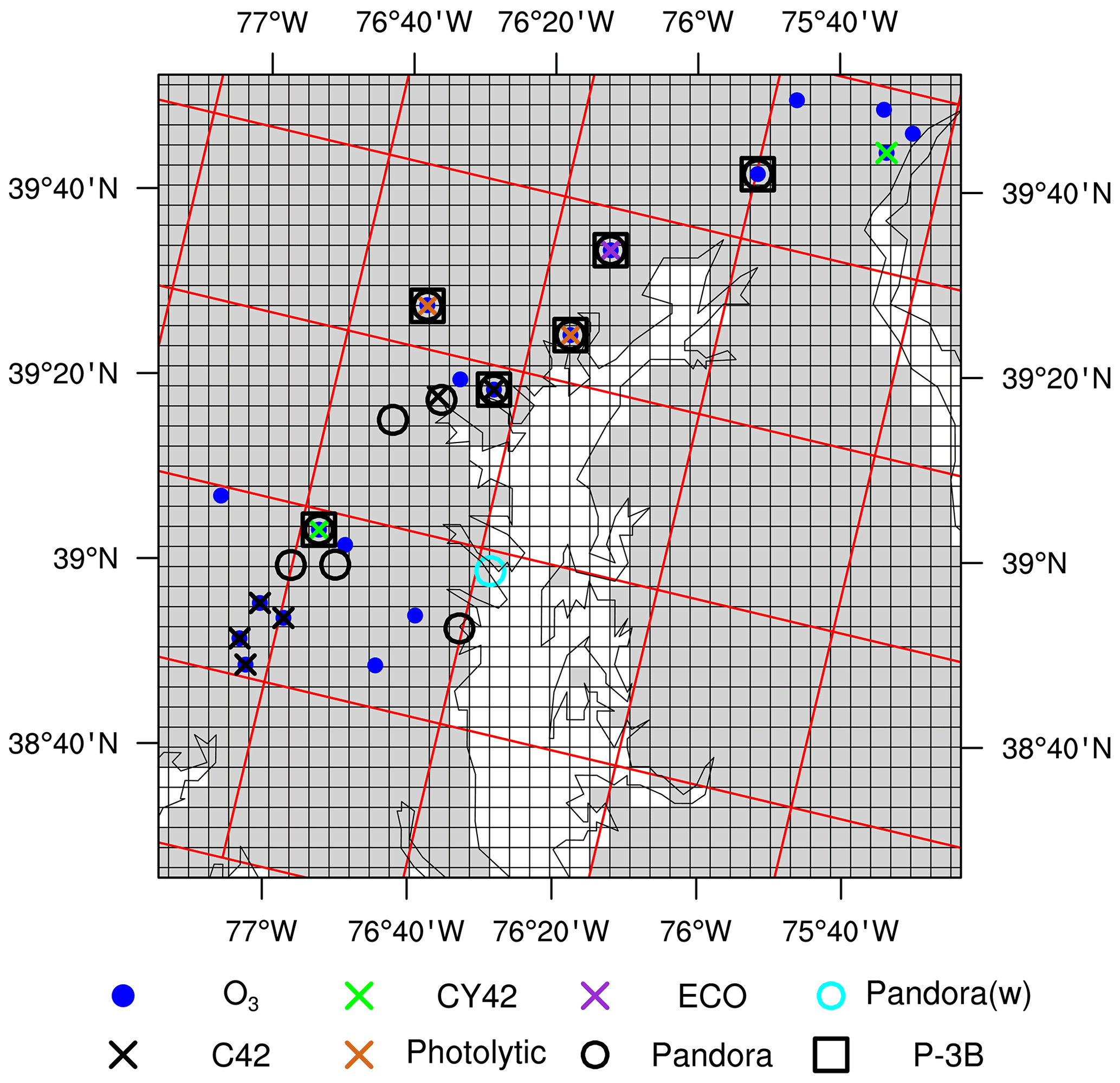
Figure 1 The locations of surface and P-3B aircraft observations during the DISCOVER-AQ 2011 campaign. We mark the 36 km REAM grid cells with red lines and the 4 km REAM grid cells with black lines. Gray shading denotes land surface in the nested 4 km WRF domain, while the white area denotes ocean or water surface. Blue dots denote surface O₃ observation sites. Cross marks denote surface NO₂ observation sites, and their colors denote different measurement instruments: green for the Thermo Electron 42C-Y NO_y analyzer, dark orchid for the Ecotech Model 9841/9843 T-NO_y analyzers, black for the Thermo Model 42C NO_x analyzer, and chocolate for the Teledyne API model 200eup photolytic NO_x analyzer. Circles denote Pandora sites, and the cyan circle denotes a Pandora site (USNA) on a ship. Black squares denote the inland P-3B aircraft spiral locations.

All of the above research, however, exploited only NO₂ surface or satellite VCD measurements. Due to the availability of ground-based NO₂ VCD observations, some recent studies tried to investigate the diurnal relationships between NO₂ surface concentrations and NO₂ VCDs (Kollonige et al., 2018; Thompson et al., 2019). For example, Zhao et al. (2019) converted Pandora direct-sun and zenith-sky NO₂ VCDs to NO₂ surface concentrations using concentration-to-partial-column ratios and found that the derived concentrations captured the observed NO₂ surface diurnal and seasonal variations well. Knepp et al. (2015) related the daytime variations in NO₂ TVCD measurements by ground-based Pandora instruments to the variations in coincident NO₂ surface concentrations using a planetary boundary layer height (PBLH) factor over the periods July 2011–October 2011 at the NASA Langley Research Center in Hampton, Virginia, and July 2011 at the Padonia and Edgewood sites in Maryland for the DISCOVER-AQ experiment, showing the importance of boundary layer vertical mixing on NO₂ vertical distributions and the ability of NO₂ VCD measurements to infer hourly boundary layer NO₂ variations. DISCOVER-AQ, the Deriving Information on Surface conditions from Column and Vertically Resolved Observations Relevant to Air Quality experiment (https://discover-aq.larc.nasa.gov/, last access: 6 April 2019), was designed to better understand the relationship between boundary layer pollutants and satellite observations (Flynn et al., 2014; Reed et al., 2015). Figure 1 shows the sampling locations of the summer DISCOVER-AQ 2011 campaign in the Baltimore–Washington metropolitan region. In this campaign, the NASA P-3B aircraft flew spirals over six air quality monitoring sites (Aldino – rural and suburban, Edgewood – coastal and urban, Beltsville – suburban, Essex – coastal and urban, Fairhill – rural, and Padonia – suburban) (Table S1 in the Supplement) and the Chesapeake Bay (Cheng et al., 2017; Lamsal et al., 2014) and measured 245 NO₂ profiles in 14 flight days in July (Zhang et al., 2016). During the same period, the NASA UC-12 aircraft flew across the Baltimore–Washington region at an altitude of about 8 km above sea level (a.s.l.), using the Airborne Compact Atmospheric Mapper (ACAM) to map the distributions of NO₂ VCDs below the aircraft (Lamsal et al., 2017). Furthermore, ground-based instruments were deployed to measure NO₂ surface concentrations, NO₂ VCDs, and other physical properties of the atmosphere (Anderson et al., 2014; Reed et al., 2015; Sawamura et al., 2014). Satellite OMI and GOME-2A (Global Ozone Monitoring Experiment – 2A) instruments provided NO₂ TVCD measurements over the campaign region at 13:30 and 09:30 LT, respectively. These concurrent measurements of NO₂ VCDs, surface NO₂, and vertically resolved distributions of NO₂ during the DISCOVER-AQ 2011 campaign, therefore, provide a comprehensive dataset to evaluate NO₂ diurnal and spatial variabilities and processes affecting NO₂ concentrations.

Section 2 describes the measurement datasets in detail. The Regional chEmistry and trAnsport Model (REAM), also described in Sect. 2, is applied to simulate the NO₂ observations during the DISCOVER-AQ campaign in July 2011. The evaluations of the simulated diurnal cycles of surface NO₂ concentrations, NO₂ vertical profiles, and NO₂ TVCDs are discussed in Sect. 3 through comparisons with observations. In Sect. 3, we also investigate the differences between NO₂ diurnal cycles on weekdays and weekends and their implications for NO_x emission characteristics. To corroborate our evaluation of NO_x emissions based on NO₂ diurnal cycles, we further compare observed NO_y (reactive nitrogen compounds) concentrations with REAM simulation results in Sect. 3. Moreover, we assess the resolution dependence of REAM simulation results in light of the observations and discuss the potential distribution biases of NO_x emissions by comparing the 36 and 4 km REAM simulation results with OMI, GOME-2A, and high-resolution ACAM NO₂ VCDs. Finally, we summarize the study in Sect. 4.

2 Datasets and model description

2.1 REAM

REAM has been widely applied in many studies (Cheng et al., 2017; Choi et al., 2008; Li et al., 2019; R. Zhang et al., 2018; Y. Zhang et al., 2016; Zhao et al., 2009). The model has a horizontal resolution of 36 km and 30 vertical layers in the troposphere. Meteorology fields are from a Weather Research and Forecasting (WRF; version 3.6) model simulation with a horizontal resolution of 36 km. We summarize the physics parameterization schemes of the WRF simulation in Table S2. The WRF simulation is initialized and constrained by the NCEP coupled forecast system model version 2 (CFSv2) products (http://rda.ucar.edu/datasets/ds094.0/, last access: 10 March 2015) (Saha et al., 2011). The chemistry mechanism in REAM is based on GEOS-Chem v11.01 with updated aerosol uptake of isoprene nitrates (Fisher et al., 2016) and revised treatment of wet scavenging processes (Luo et al., 2019). A 2^∘ × 2.5^∘ GEOS-Chem simulation provides the chemical boundary and initial conditions.

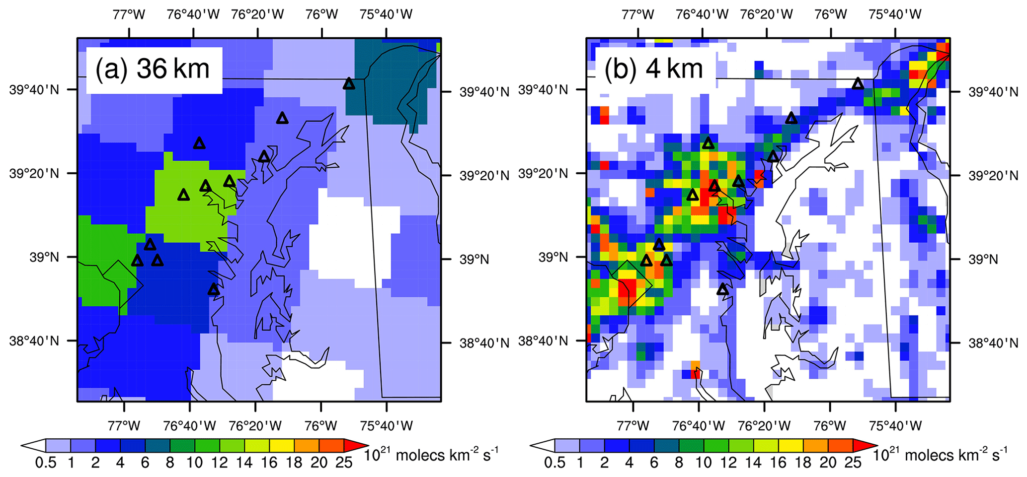
Figure 2 Distributions of NO_x emissions for the (a) 36 km and (b) 4 km REAM simulations around the DISCOVER-AQ 2011 region. Here NO_x emissions refer to the mean values ($\mathrm{molecules}{\mathrm{km}}^{-\mathrm{2}}{\mathrm{s}}^{-\mathrm{1}}$) in 1 week (Monday–Sunday).

Figure 3 Relative diurnal profiles of weekday and weekend NO_x emissions ($\mathrm{molecules}{\mathrm{km}}^{-\mathrm{2}}{\mathrm{s}}^{-\mathrm{1}}$) in the DISCOVER-AQ 2011 region (the 36 and 4 km grid cells over the 11 inland Pandora sites shown in Fig. 1) for the 36 and 4 km REAM. All the profiles are scaled by the 4 km weekday emission average value ($\mathrm{molecules}{\mathrm{km}}^{-\mathrm{2}}{\mathrm{s}}^{-\mathrm{1}}$).

Biogenic VOC emissions in REAM are from MEGAN v2.10 (Guenther et al., 2012). Anthropogenic emissions on weekdays are from the National Emission Inventory 2011 (NEI2011) (EPA, 2014) from the Pacific Northwest National Laboratory (PNNL), which has an initial resolution of 4 km and is regridded to REAM 36 km grid cells (Fig. 2). Weekday emission diurnal profiles are from NEI2011. The weekday-to-weekend emission ratios and weekend emission diurnal profiles are based on previous studies (Beirle et al., 2003; Boersma et al., 2009; Choi et al., 2012; de Foy, 2018; DenBleyker et al., 2012; Herman et al., 2009; Judd et al., 2018; Kaynak et al., 2009; Kim et al., 2016). These studies suggested that weekend NO_x emissions were 20 %–50 % lower than weekday emissions, and the weekend NO_x emission diurnal cycles were different from weekdays; therefore, we specify a weekend-to-weekday NO_x emission ratio of $\mathrm{2}/\mathrm{3}$ in this study. The resulting diurnal variations in weekday and weekend NO_x emissions over the DISCOVER-AQ 2011 region are shown in Fig. 3. The diurnal emission variation is lower on weekends than on weekdays.

To understand the effects of model resolutions on the temporospatial distributions of NO₂, we also conduct a REAM simulation with a horizontal resolution of 4 km during the DISCOVER-AQ campaign. A 36 km REAM simulation (discussed in Sect. 3.2) provides the chemical initial and hourly boundary conditions. Meteorology fields are from a nested WRF simulation (36, 12, 4 km) with cumulus parameterization turned off in the 4 km domain (Table S2). Figure 1 shows a comparison of the 4 and 36 km REAM grid cells with DISCOVER-AQ observations, and Fig. 2 shows a comparison of NO_x emission distributions between the 4 and 36 km REAM simulations. The comparison of NO_x emission diurnal variations over the DISCOVER-AQ 2011 region between the 4 and 36 km REAM is shown in Fig. 3.

2.2 NO₂ TVCD measurements by OMI and GOME-2A

The OMI instrument onboard the sun-synchronous NASA EOS Aura satellite with an Equator-crossing time of around 13:30 LT was developed by the Finnish Meteorological Institute and the Netherlands Agency for Aerospace Programs to measure solar backscattering radiation in the visible and ultraviolet bands (Levelt et al., 2006; Russell et al., 2012). The radiance measurements are used to derive trace gas concentrations in the atmosphere, such as O₃, NO₂, HCHO, and SO₂ (Levelt et al., 2006). OMI has a nadir resolution of 13 km × 24 km and provides daily global coverage (Levelt et al., 2006).

Two widely used archives of OMI NO₂ VCD products are available, NASA OMNO2 (v4.0) (https://disc.gsfc.nasa.gov/datasets/OMNO2_003/summary, last access: 26 September 2020) and KNMI DOMINO (v2.0) (https://www.temis.nl/airpollution/no2.php, last access: 14 January 2015). Although both use Differential Optical Absorption Spectroscopy (DOAS) algorithms to derive NO₂ slant column densities, they have differences in spectral fitting, stratospheric and tropospheric NO₂ slant column density (SCD) separation, a priori NO₂ vertical profiles, air mass factor (AMF) calculation, etc. (Boersma et al., 2011; Bucsela et al., 2013; Chance, 2002; Krotkov et al., 2017; Lamsal et al., 2021; Marchenko et al., 2015; Oetjen et al., 2013; van der A et al., 2010; Van Geffen et al., 2015). Both OMNO2 and DOMINO have been extensively evaluated with field measurements and models (Boersma et al., 2009, 2011; Choi et al., 2020; Hains et al., 2010; Huijnen et al., 2010; Ionov et al., 2008; Irie et al., 2008; Lamsal et al., 2014, 2021; Oetjen et al., 2013). The estimated uncertainty in the DOMINO TVCD product includes an absolute component of 1.0 × 10¹⁵ molecules cm⁻² and a relative AMF component of 25 % (Boersma et al., 2011), while the uncertainty in the OMNO2 TVCD product ranges from ∼ 30 % under clear-sky conditions to ∼ 60 % under cloudy conditions (Lamsal et al., 2014; Oetjen et al., 2013; Tong et al., 2015). In order to reduce uncertainties in this study, we only use TVCD data with effective cloud fractions < 0.2, solar zenith angle (SZA) < 80^∘, and albedo ≤ 0.3. Both positive and negative TVCDs are considered in the calculation. The data affected by row anomaly are excluded (Boersma et al., 2018; R. Zhang et al., 2018).

For AMF calculation, DOMINO used daily TM4 model results with a resolution of 3^∘ × 2^∘ as a priori NO₂ vertical profiles (Boersma et al., 2007, 2011), while OMNO2 v4.0 used monthly mean values from the Global Modeling Initiative (GMI) model with a resolution of 1^∘ × 1.25^∘. The relatively coarse horizontal resolution of the a priori NO₂ profiles in the retrievals can introduce uncertainties in the spatial and temporal characteristics of NO₂ TVCDs at satellite pixel scales. For comparison purposes, we also use 36 km REAM simulation results as the a priori NO₂ profiles to compute the AMFs and NO₂ TVCDs with the DOMINO algorithm. The 36 km REAM NO₂ data are first regridded to OMI pixels to calculate the corresponding tropospheric AMFs, which are then applied to compute OMI NO₂ TVCDs by dividing the tropospheric SCDs from the DOMINO product by our updated AMFs.

The GOME-2 instrument onboard the polar-orbiting MetOp-A satellite (now referred to as GOME-2A) is an improved version of GOME-1 launched in 1995 and has an overpass time of 09:30 LT and a spatial resolution of 80 km × 40 km (Munro et al., 2006; Peters et al., 2012). GOME-2A measures backscattered solar radiation in the range from 240 to 790 nm, which is used for VCD retrievals of trace gases, such as O₃, NO₂, BrO, and SO₂ (Munro et al., 2006). We use the KNMI TM4NO2A v2.3 GOME-2A NO₂ VCD product archived on http://www.temis.nl/airpollution/no2col/no2colgome2_v2.php (last access: 22 January 2015) (Boersma et al., 2007, 2011). GOME-2A-derived NO₂ VCDs have been validated with SCIAMACHY and MAX-DOAS measurements (Irie et al., 2012; Peters et al., 2012; Richter et al., 2011). As in the case of OMI, we use the same criteria to filter the NO₂ TVCD data and recalculate the tropospheric AMF values and GOME-2A TVCDs using the daily 36 km REAM NO₂ profiles (09:00–10:00 LT).

2.3 Pandora ground-based NO₂ VCD measurements

Pandora is a small direct sun spectrometer which measures sun and sky radiance from 270 to 530 nm with a 0.5 nm resolution and a 1.6^∘ field of view (FOV) for the retrieval of the total VCDs of NO₂ with a precision of about 5.4 × 10¹⁴ molecules cm⁻² (2.7 × 10¹⁴ molecules cm⁻² for NO₂ SCD) and a nominal accuracy of 2.7 × 10¹⁵ molecules cm⁻² under clear-sky conditions (Herman et al., 2009; Lamsal et al., 2014; Zhao et al., 2020). There were 12 Pandora sites operating in the DISCOVER-AQ campaign (Fig. 1). Six of them are the same as the P-3B aircraft spiral locations (Aldino, Edgewood, Beltsville, Essex, Fairhill, and Padonia) (Table S1 and Fig. 1). The other six sites are Naval Academy (Annapolis, Maryland) (USNA – ocean), University of Maryland College Park (UMCP – urban), University of Maryland Baltimore County (UMBC – urban), Smithsonian Environmental Research Center (SERC – rural and coastal), Oldtown in Baltimore (Oldtown – urban), and Goddard Space Flight Center (GSFC – urban and suburban) (Table S1 and Fig. 1). In this study, we exclude the USNA site as its measurements were conducted on a ship (“Pandora(w)” in Fig. 1), and there were no other surface observations in the corresponding REAM grid cell. Including the data from the USNA site has a negligible effect on the comparisons of observed and simulated NO₂ TVCDs. In our analysis, we ignore Pandora measurements with SZA > 80^∘ (Fig. S1 in the Supplement) and exclude the data when fewer than three valid measurements are available within an hour to reduce the uncertainties in the hourly averages due to the significant variations in Pandora observations (Fig. S2).

Since Pandora measures total NO₂ VCDs, we need to subtract stratosphere NO₂ VCDs from the total VCDs to compute TVCDs. As shown in Fig. S3, stratosphere NO₂ VCDs show a clear diurnal cycle with an increase during daytime due in part to the photolysis of reactive nitrogen reservoirs such as N₂O₅ and HNO₃ (Brohede et al., 2007; Dirksen et al., 2011; Peters et al., 2012; Sen et al., 1998; Spinei et al., 2014), which is consistent with the significant increase in stratospheric NO₂ VCDs from GOME-2A to OMI. In this study, we use the GMI model-simulated stratospheric NO₂ VCDs in Fig. S3 to calculate the Pandora NO₂ TVCDs. The small discrepancies between the GMI stratospheric NO₂ VCDs and satellite products do not change the pattern of Pandora NO₂ TVCD diurnal variations or affect the conclusions in this study.

2.4 ACAM NO₂ VCD measurements

The ACAM instrument onboard the UC-12 aircraft consists of two thermally stabilized spectrometers in the ultraviolet, visible, and near-infrared range. The spectrometer in the ultraviolet and visible band (304–520 nm) with a resolution of 0.8 nm and a sampling of 0.105 nm can be used to detect NO₂ in the atmosphere. The native ground resolution of UC-12 ACAM NO₂ measurements is 0.5 km × 0.75 km at a flight altitude of about 8 km a.s.l. and a nominal ground speed of 100 m s⁻¹ during the DISCOVER-AQ 2011 campaign (Lamsal et al., 2017), thus providing high-resolution NO₂ VCDs below the aircraft.

In this study, we mainly use the ACAM NO₂ VCD product described by Lamsal et al. (2017), which applied a pair-average co-adding scheme to produce NO₂ VCDs at a ground resolution of about 1.5 km (cross-track) × 1.1 km (along-track) to reduce noise impacts. In their retrieval of ACAM NO₂ VCDs, they first used the DOAS fitting method to generate differential NO₂ SCDs relative to the SCDs at an unpolluted reference location. Then they computed above- and below-aircraft AMFs at both sampling and reference locations based on the vector linearized discrete ordinate radiative transfer code (VLIDORT) (Spurr, 2008). In the computation of AMFs, the a priori NO₂ vertical profiles were from a combination of high-resolution (4 km) CMAQ (the Community Multiscale Air Quality Modeling System) model outputs in the boundary layer and GMI simulation (2^∘ × 2.5^∘) results elsewhere in the atmosphere. Finally, the below-aircraft NO₂ VCDs at the sampling locations were generated by dividing below-aircraft NO₂ SCDs at the sampling locations by the corresponding below-aircraft AMFs. The below-aircraft NO₂ SCDs were the differences between the total and above-aircraft NO₂ SCDs. The total NO₂ SCDs were the sum of DOAS-fitting-generated differential NO₂ SCDs and NO₂ SCDs at the reference location, and the above-aircraft NO₂ SCDs were derived based on above-aircraft AMFs, GMI NO₂ profiles, and OMNO2 stratospheric NO₂ VCDs (Lamsal et al., 2017). The ACAM NO₂ VCD product had been evaluated via comparisons with other independent observations during the DISCOVER-AQ 2011 campaign, such as P-3B aircraft, Pandora, and OMNO2, and the uncertainty in individual below-aircraft NO₂ VCD is about 30 % (Lamsal et al., 2017). To keep the consistency of ACAM NO₂ VCDs, we exclude NO₂ VCDs measured at altitudes <8 km a.s.l., which accounts for about 6.8 % of the total available ACAM NO₂ VCD data. We regrid the 1.5 km×1.1 km ACAM NO₂ VCDs to the 4 km REAM grid cells (Fig. 1), which are then used to evaluate the distribution of NO₂ VCDs in the 4 km REAM simulation. As a supplement in Sect. 3.7, we also assess the 4 km REAM simulation by using the UC-12 ACAM NO₂ VCDs produced by the Smithsonian Astrophysical Observatory (SAO) algorithms, archived on https://www-air.larc.nasa.gov/cgi-bin/ArcView/discover-aq.dc-2011?UC12=1#LIU.XIONG/ (last access: December 31, 2019) (Liu et al., 2015a, b). This product is an early version of the SAO algorithm used to produce the Geostationary Trace gas and Aerosol Sensor Optimization (GeoTASO) and the GEOstationary Coastal and Air Pollution Events (GEO-CAPE) Airborne Simulator (GCAS) airborne observations in later airborne campaigns (Nowlan et al., 2016, 2018).

2.5 Surface NO₂ and O₃ measurements

The measurement of NO_x is based on the chemiluminescence of electronically excited ${\mathrm{NO}}_{\mathrm{2}}^{\ast }$, produced from the reaction of NO with O₃, and the strength of the chemiluminescence from the decay of ${\mathrm{NO}}_{\mathrm{2}}^{\ast }$ to NO₂ is proportional to the number of NO molecules present (Reed et al., 2016). NO₂ concentrations can be measured with this method by converting NO₂ to NO first through catalytic reactions (typically on the surface of heated molybdenum oxide (MoO_x) substrate) or photolytic processes (Lamsal et al., 2015; Reed et al., 2016). However, for the catalytic method, reactive nitrogen compounds other than NO_x (NO_z), such as HNO₃, peroxyacetyl nitrate (PAN), and other organic nitrates, can also be reduced to NO on the heated surface, thus causing an overestimation of NO₂. The magnitude of the overestimation depends on the concentrations and the reduction efficiencies of interference species, both of which are uncertain. The photolytic approach, which employs broadband photolysis of ambient NO₂, offers more accurate NO₂ measurements (Lamsal et al., 2015).

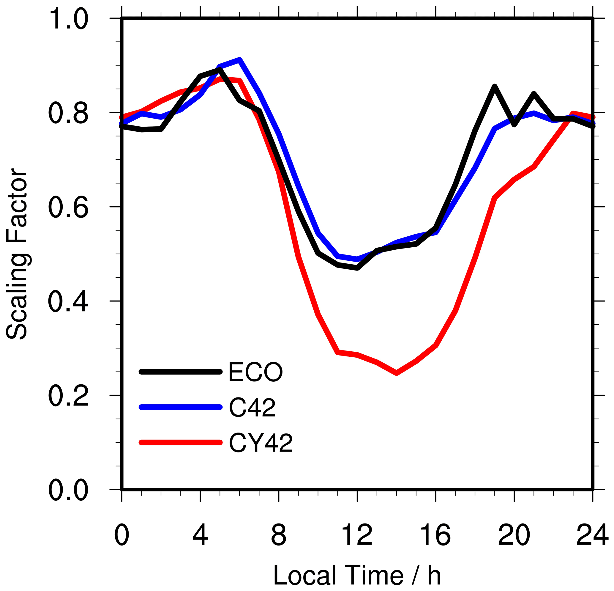
Figure 4 Hourly ratios of NO₂ measurements from the Teledyne API model 200 eup photolytic NO_x analyzer to NO₂ from coincident catalytic instruments for 2011 July. “CY42” denotes the ratios of photolytic NO₂ to NO₂ from the Thermo Electron 42C-Y NO_y analyzer in Edgewood, “C42” denotes the ratios of photolytic NO₂ to NO₂ from the Thermo Model 42C NO_x analyzer in Padonia, and “ECO” denotes the ratios of photolytic NO₂ to NO₂ from the Ecotech Model 9841 T-NO_y analyzer in Padonia. “ECO” ratios are also used to scale NO₂ measurements from the Ecotech Model 9843 T-NO_y analyzer.

There were 11 NO_x monitoring sites operating in the DISCOVER-AQ region during the campaign (Fig. 1), including those from the EPA Air Quality System (AQS) monitoring network and those deployed for the DISCOVER-AQ campaign. Nine of them measured NO₂ concentrations by a catalytic converter. The other two sites (Edgewood and Padonia) had NO₂ measurements from both catalytic and photolytic methods. Different stationary catalytic instruments were used during the campaign: Thermo Electron 42C-Y NO_y analyzer, Thermo Model 42C NO_x analyzer, Thermo Model 42I-Y NO_y analyzer, and Ecotech Model 9843 and 9841 T-NO_y analyzers. In addition, a mobile platform – NATIVE (Nittany Atmospheric Trailer and Integrated Validation Experiment) with a Thermo Electron 42C-Y NO_y analyzer installed – was also deployed at the Edgewood site. The photolytic measurements of NO₂ in Edgewood and Padonia were from Teledyne API model 200eup photolytic NO_x analyzers. We scale catalytic NO₂ measurements using the diurnal ratios of NO₂ photolytic measurements to NO₂ from the corresponding catalytic analyzers (Fig. 4). Figure 4 shows the lowest photolytic–catalytic ratio in the afternoon, which reflects the production of nitrates and other reactive nitrogen compounds from NO_x in the daytime. When photolytic measurements are available, we only use the photolytic observations in this study; otherwise, we use the scaled catalytic measurements.

Nineteen surface O₃ monitoring sites were operating in the DISCOVER-AQ region during the campaign (Fig. 1). They measured O₃ concentrations by using a federal equivalent method (FEM) based on the UV absorption of O₃ (https://cfpub.epa.gov/si/si_public_file_download.cfm?p_download_id=520887&Lab=NERL, last access: 12 July 2021) with an uncertainty of 5 ppb.

2.6 Aircraft measurements of NO₂ vertical profiles

In this study, we mainly use the NO₂ concentrations measured by the National Center for Atmospheric Research (NCAR) four-channel chemiluminescence instrument (P-CL) onboard the P-3B aircraft for the evaluation of REAM-simulated NO₂ vertical profiles. The instrument has an NO₂ measurement uncertainty of 10 %–15 % and a 1 s, 1σ detection limit of 30 pptv.

NO₂ measurements from aircraft spirals provide us with NO₂ vertical profiles. Figure 1 shows the locations of the aircraft spirals during the DISCOVER-AQ campaign, except for the Chesapeake Bay spirals over the ocean. There were only six spirals available over the Chesapeake Bay, which have ignorable impacts on the following analyses. Therefore, we do not use them in this study. The remaining 239 spirals in the daytime for July 2011 are used to compute the average profiles of NO₂ for the six inland sites (Fig. 1).

The aircraft measurements were generally sampled from a height of about 300 $\mathrm{m}\mathrm{a}.\mathrm{g}.\mathrm{l}.$ (above ground level) in the boundary layer to 3.63 $\mathrm{km}\mathrm{a}.\mathrm{g}.\mathrm{l}.$ in the free troposphere. We bin these measurements to REAM vertical levels. In order to make up the missing observations between the surface and 300 m, we apply quadratic polynomial regressions by using aircraft data below 1 km and coincident NO₂ surface measurements.

Table 1 Comparison of the concentrations of NO_y and its components between REAM and P-3B aircraft measurements during the DISCOVER-AQ campaign.

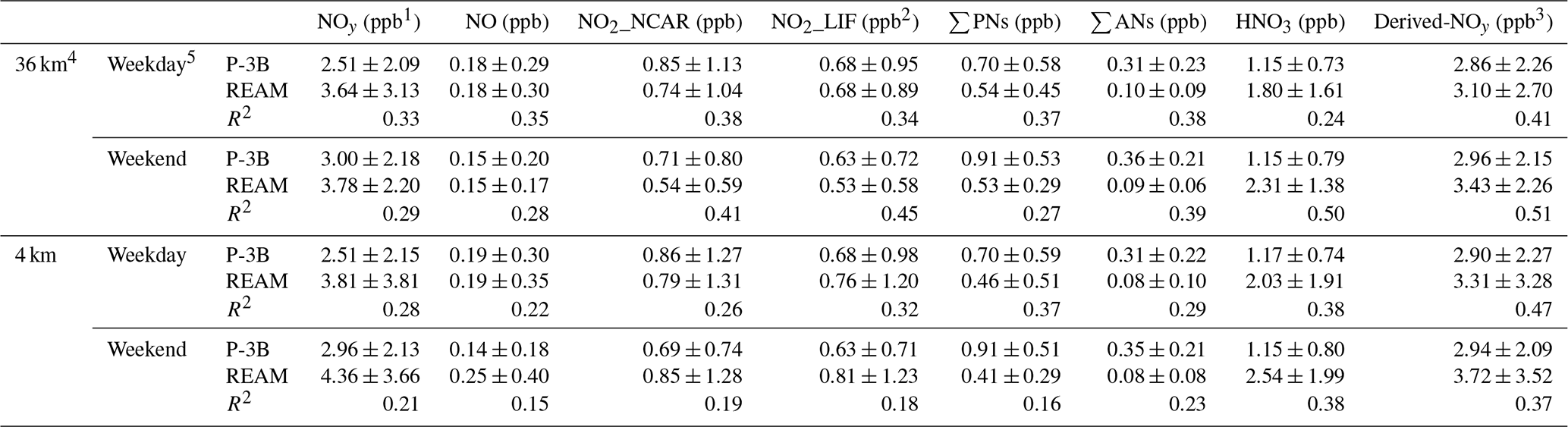
¹ For P-3B, the concentrations of NO_y, NO, and NO₂_NCAR were measured by using the NCAR four-channel chemiluminescence instrument. The measurement uncertainties are 10 %, 10 %–15 %, and 10 % for NO, NO₂, and NO_y, respectively. The 1 s, 1σ detection limits are 20, 30, and 20 pptv for NO, NO₂, and NO_y, respectively (https://discover-aq.larc.nasa.gov/wp-content/uploads/sites/140/2020/05/Weinheimer20101005_DISCOVERAQ_AJW.pdf, last access: 28 June 2019). For REAM, NO_y is the sum of NO, NO₂, total peroxyacyl nitrates (∑PNs), total alkyl nitrates (∑ANs) (including alkyl nitrates and hydroxyalkyl nitrates), HNO₃, HONO, 2 × N₂O₅, HNO₄, first-generation C5 carbonyl nitrate (nighttime isoprene nitrate ISN1: C₅H₈NO₄), 2 × C5 dihydroxy dinitrate (DHDN: C₅H₁₀O₈N₂), methyl peroxy nitrate (MPN: CH₃O₂NO₂), propanone nitrate (PROPNN: CH₃C(=O)CH₂ONO₂), nitrate from methyl vinyl ketone (MVKN: HOCH₂CH(ONO₂)C(=O)CH₃), nitrate from methacrolein (MARCN: HOCH₂C(ONO₂)(CH₃)CHO), and ethanol nitrate (ETHLN: CHOCH₂ONO₂).
² For P-3B, the concentrations of NO₂_LIF, ∑PNs, ∑ANs, and HNO₃ were measured by applying the thermal-dissociation laser-induced fluorescence (TD-LIF) technique. The accuracy of TD-LIF measurements of NO₂, ∑PNs, ∑ANs, and HNO₃ is better than 15 %, and the detection limit for the sum of NO₂, ∑PNs, ∑ANs, and HNO₃ is ∼ 10 ppt 10 s⁻¹ (Day et al., 2002).
³ To compare NO_y concentrations from TD-LIF measurements with those from REAM, we calculate derived-NO_y as the sum of NO, NO₂_LIF, ∑PNs, ∑ANs, and HNO₃. Only when the concentrations of all the five species are available at the same hour in the same grid cell can we calculate derived-NO_y at the given hour in the given grid cell. Therefore, in Table 1, the averaged derived-NO_y values are not exactly equal to the sum of averaged NO, NO₂_LIF, ∑PNs, ∑ANs, and HNO₃ concentrations that only depend on the availability of a single species. In addition, the measurement times and frequencies between NO_y and derived-NO_y are not the same. A comparison between these two types of data needs coincident sampling, as described in the main text.
⁴ Mean NO_x emissions over the six P-3B spiral sites are close (relative difference < 4 %) between the 36 and 4 km REAM (Table S1).
⁵ Due to different sampling times and locations between weekdays and weekends, we do not recommend a direct comparison between weekday and weekend values here.

In addition to using NO₂ concentrations from the NCAR four-channel instrument to evaluate REAM-simulated NO₂ vertical profiles, we also use P-3B NO, NO₂, and NO_y concentrations measured by the NCAR four-channel instrument and NO₂, total peroxyacyl nitrates (∑PNs), total alkyl nitrates (∑ANs) (including alkyl nitrates and hydroxyalkyl nitrates), and HNO₃ concentrations measured by the thermal-dissociation laser-induced fluorescence (TD-LIF) technique (Day et al., 2002; Thornton et al., 2000; Wooldridge et al., 2010) to evaluate the concentrations of NO_y from REAM (Table 1). All these P-3B measurements are vertically binned to REAM grid cells for comparisons with REAM results. In addition, below the P-3B spirals, four NO_y observation sites at Padonia, Edgewood, Beltsville, and Aldino were operating to provide continuous hourly NO_y surface concentrations during the campaign, which we also use to evaluate REAM-simulated NO_y surface concentrations in this study. We summarize the information of available observations at the 11 inland Pandora sites in Table S1.

3 Results and discussion

3.1 Evaluation of WRF-simulated meteorological fields

We evaluate the performances of the 36 km and nested 4 km WRF simulations using temperature, potential temperature, relative humidity (RH), and wind measurements from the P-3B spirals (Fig. 1) and precipitation data from the NCEP (National Centers for Environmental Prediction) Stage IV precipitation dataset. Generally, P-3B spirals range from ∼ 300 m to ∼ 3.63 km in height above the ground level (a.g.l.). As shown in Fig. S4, both the 36 km and nested 4 km WRF simulations simulate temperature well with R² = 0.98. Both WRF simulations show good agreement with P-3B measurements in U wind (36 km: R² = 0.77; 4 km: R² = 0.76), V wind (36 km: R² = 0.79; 4 km: R² = 0.78), wind speed (36 km: R² = 0.67; 4 km: R² = 0.67), and wind direction (Figs. S4 and S5). We further compare the temporal evolutions of vertical profiles for temperature, potential temperature, RH, U wind, and V wind below 3 km from the P-3B observations with those from the 36 km and nested 4 km WRF simulations in Fig. S6. Both WRF simulations capture the temporospatial variations in P-3B-observed vertical profiles well except that RH below 1.5 km is significantly underestimated between 09:00 and 17:00 LT in both WRF simulations. The evaluations above suggest that WRF-simulated wind fields are good and comparable at 4 and 36 km resolutions, but potential dry biases exist in both WRF simulations.

The NCEP Stage IV precipitation dataset provides hourly precipitation across the contiguous United States (CONUS) with a resolution of ∼ 4 km based on the merging of rain gauge data and radar observations (Lin and Mitchell, 2005; Nelson et al., 2016). The Stage IV dataset is useful for evaluating model simulations, satellite precipitation estimates, and radar precipitation estimates (Davis et al., 2006; Gourley et al., 2011; Kalinga and Gan, 2010; Lopez, 2011; Yuan et al., 2008). We obtain the Stage IV precipitation data for July 2011 from the NCAR/UCAR Research Data Archive (https://rda.ucar.edu/datasets/ds507.5/, last access: 28 December 2019). As shown in Figs. S7 and S8, both the 36 km and nested 4 km WRF simulations generally predict much less precipitation (in precipitation amount and duration) compared to the Stage IV data in July 2011 around the DISCOVER-AQ campaign region, especially for the nested 4 km WRF simulation, consistent with the aforementioned underestimated RH and dry bias in WRF simulations. The precipitation biases in the WRF model will affect REAM simulations of trace gases, leading to high biases of soluble species due to underestimated wet scavenging. Clouds interfere with satellite observations. Therefore, the precipitation bias does not affect model evaluations with satellite measurements of NO₂. Aircraft measurements were also taken on non-precipitating days.

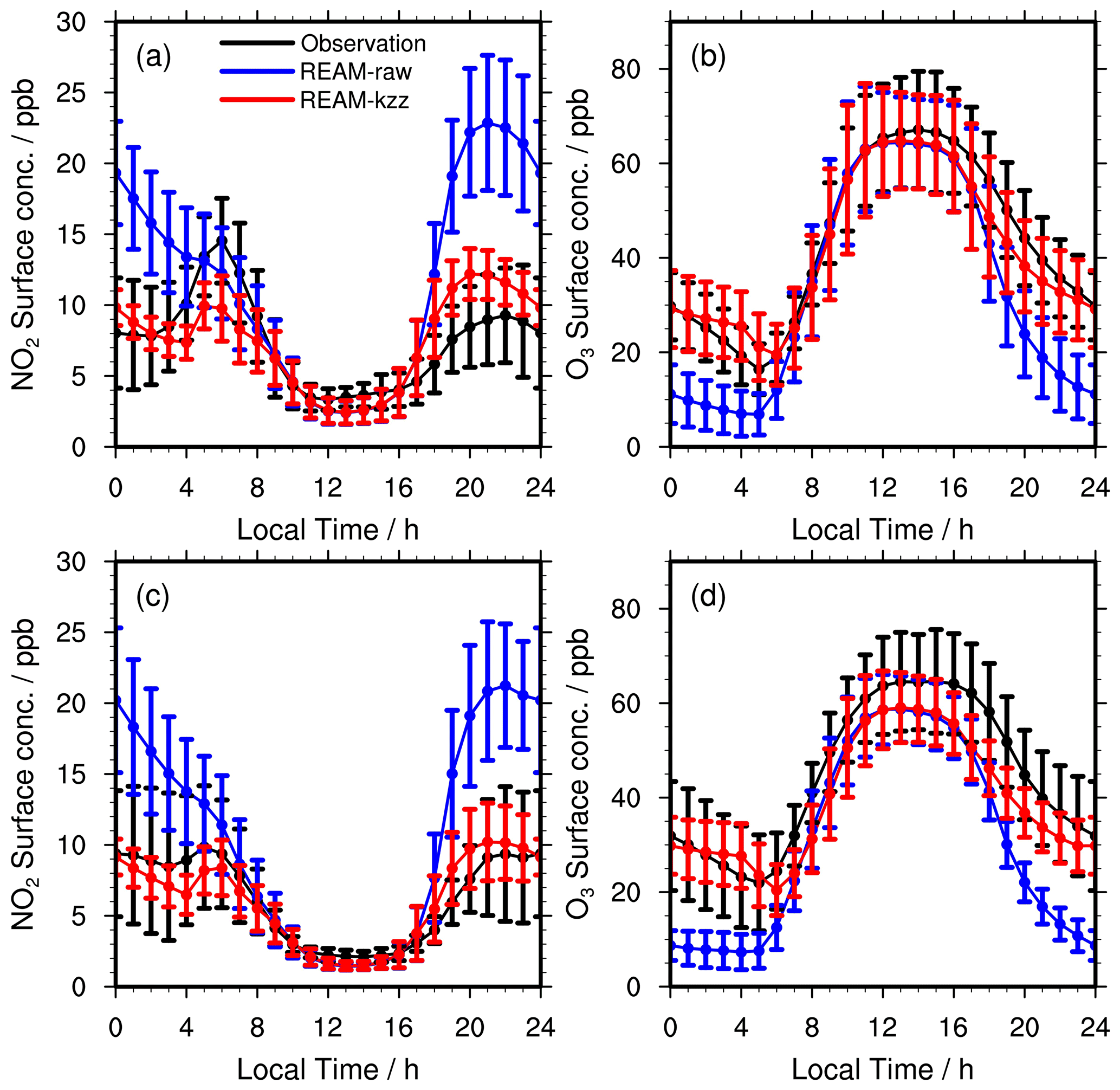
Figure 5 Diurnal cycles of surface (a, c) NO₂ and (b, d) O₃ concentrations on (a, b) weekdays and (c, d) weekends during the DISCOVER-AQ campaign in the DISCOVER-AQ region (the 36 km grid cells over the 11 inland Pandora sites shown in Fig. 1). Black lines denote the mean observations from all the 11 NO₂ surface monitoring sites and 19 O₃ surface sites during the campaign (Fig. 1), as mentioned in Sect. 2.5. “REAM-raw” (blue lines) denotes the coincident 36 km REAM simulation results with WRF-YSU-simulated k_zz data, and “REAM-kzz” (red lines) is the coincident 36 km REAM simulation results with updated k_zz data. See the main text for details. Vertical bars denote corresponding standard deviations.

3.2 Effect of boundary layer vertical mixing on the diurnal variations in surface NO₂ concentrations

3.2.1 36 km model simulation in comparison to the surface observations

Figure 5a and b show the observed and 36 km REAM-simulated diurnal cycles of surface NO₂ and O₃ concentrations on weekdays in July 2011 in the DISCOVER-AQ region. REAM with WRF-YSU-simulated vertical diffusion coefficient (k_zz) values significantly overestimates NO₂ concentrations and underestimates O₃ concentrations at night, although it captures the patterns of the diurnal cycles of surface NO₂ and O₃: an O₃ peak and an NO₂ minimum around noontime. Here, YSU denotes the Yonsei University planetary boundary layer (PBL) scheme (Shin and Hong, 2011) used by our WRF simulations (Table S2). At night, the reaction of O₃ + NO → O₂ + NO₂ produces NO₂ but removes O₃. Since most NO_x emissions are in the form of NO, the model biases of low O₃ and high NO₂ occur at the same time. Since there are no significant chemical sources of O₃ at night, mixing of O₃-rich air above the surface is the main source of O₃ supply near the surface. Therefore, the nighttime model biases with WRF-YSU-simulated k_zz data in Fig. 5 indicate that vertical mixing may be underestimated at night.

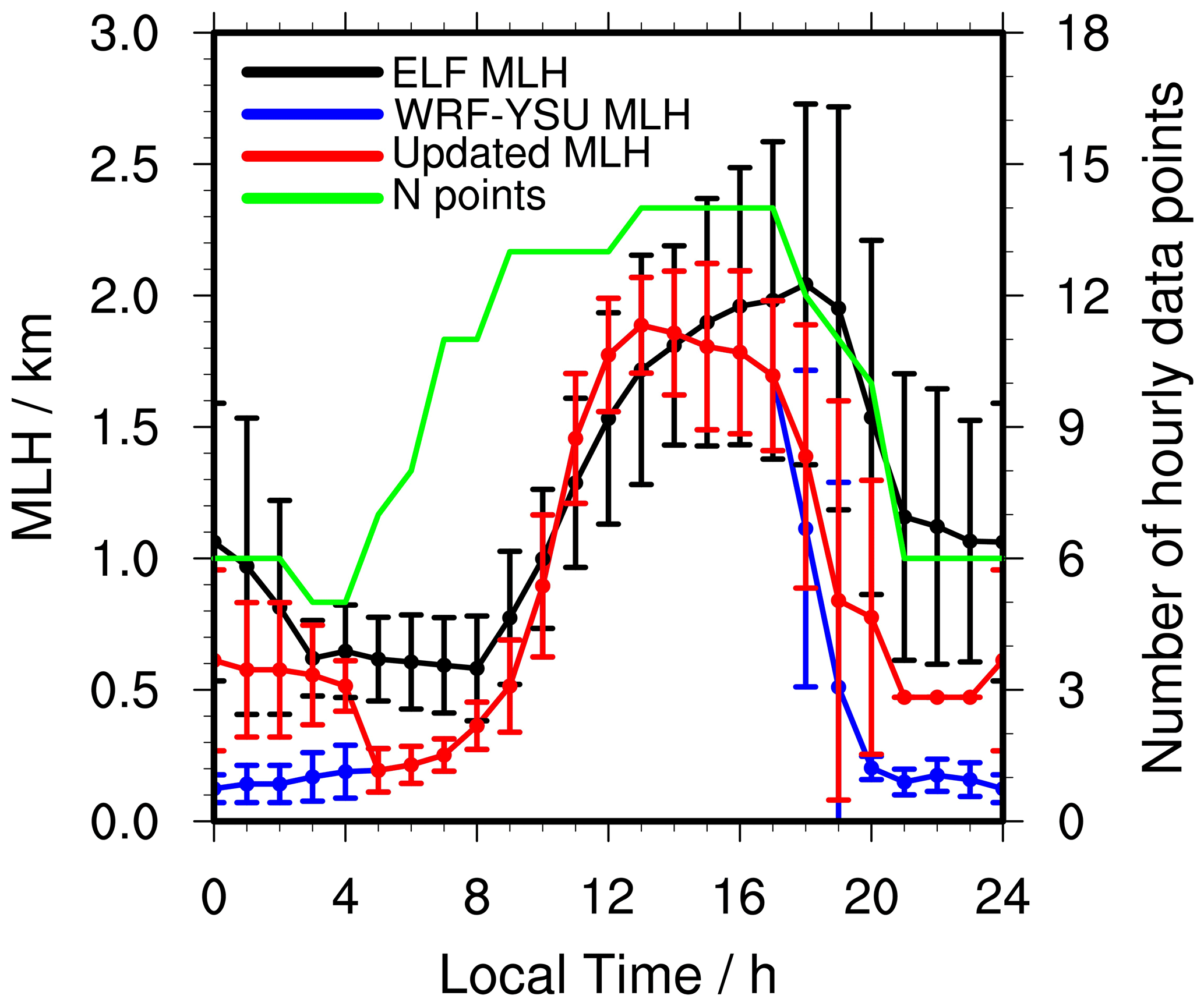
Figure 6 ELF-observed and model-simulated diurnal variations in MLH at the UMBC site during the Discover-AQ campaign. “ELF MLH” denotes ELF-derived MLHs by using the covariance wavelet transform method. “WRF-YSU MLH” denotes the 36 km WRF-YSU k_zz-determined MLHs, and “Updated MLH” denotes updated k_zz-determined MLHs. See the main text for details. Vertical bars denote standard deviations. For the ELF MLHs, there are 13 506 1 min measurements in total during the campaign, and we bin them into hourly data. The green line corresponding to the right y axis shows the diurnal variations in the number of hourly ELF data points.

During the DISCOVER-AQ campaign, WRF-simulated vertical wind velocities are very low at night and have little impact on vertical mixing (Fig. S9a). The nighttime vertical mixing is mainly attributed to turbulent mixing. However, Hu et al. (2012) found that the YSU scheme underestimated nighttime PBL vertical turbulent mixing in WRF, which is consistent with Fig. 6, showing that WRF-YSU k_zz-determined mixed-layer heights (MLHs) are significantly lower than lidar observations in the late afternoon and at night at the UMBC site during the DISCOVER-AQ campaign (Knepp et al., 2017). Here, the k_zz-determined MLH refers to the mixing height derived by comparing k_zz to its background values (Hong et al., 2006) but not the PBLH outputs from WRF. UMBC is an urban site (Table S1), surrounded by a mixture of constructed materials and vegetation. The UMBC lidar MLH data were derived from the Elastic Lidar Facility (ELF) attenuated backscatter signals by using the covariance wavelet transform (CWT) method and had been validated against radiosonde measurements (N (number of data points) = 24; R² = 0.89; bias (ELF – radiosonde) = 0.03 ± 0.23 km), radar wind profiler observations (N = 659; R² = 0.78; bias = −0.21 ± 0.36 km), and Sigma Space mini-micropulse lidar data (N = 8122; R² = 0.85; bias = 0.02 ± 0.22 km) from the Howard University Beltsville Research Campus (HUBRC) in Beltsville, Maryland (38.058^∘ N, 76.888^∘ W) in the daytime during the DISCOVER-AQ campaign (Compton et al., 2013). It is noteworthy that although CWT is not designed to detect the nocturnal boundary layer (NBL), it does consider the residue layer (RL) and distinguish it from MLH in the early morning after sunrise, which is similar to nighttime conditions. Therefore, CWT can detect nighttime MLHs, although with large uncertainties due to the hard-coded assumption of RL = 1 km in the algorithm and insufficient vertical resolution of the technique. In addition, the sunrise and sunset time in July 2011 is about 05:00 and 19:30 LT (https://gml.noaa.gov/grad/solcalc/sunrise.html, last access: 27 May 2021), respectively. Figure 6 shows that WRF-YSU k_zz-determined MLHs are significantly lower than ELF observations after sunrise between 05:00 and 08:00 LT and before sunset between 18:00 and 20:00 LT. Even if we do not consider MLHs at night (19:30–05:00 LT), we can still conclude that WRF-YSU underestimates vertical mixing in the early morning after sunrise and the late afternoon before sunset, enabling a reasonable assumption that WRF-YSU also underestimates nighttime vertical mixing. Moreover, the nighttime MLHs in Fig. 6 are comparable to those measured by the Vaisala CL51 ceilometer at the Chemistry And Physics of the Atmospheric Boundary Layer Experiment (CAPABLE) site in Hampton, Virginia (Knepp et al., 2017). Finally, we want to emphasize that different definitions of NBL can result in significantly different NBL heights (Breuer et al., 2014). In this study, we follow Knepp et al. (2017) to use MLHs derived from aerosol backscatter signals as the measure of vertical pollutant mixing within the boundary layer, which is simulated by k_zz in REAM.

To improve nighttime PBL vertical turbulent mixing in REAM, we increase k_zz below 500 m between 18:00 and 05:00 LT to 5 m s⁻² if the WRF-YSU-computed k_zz < 5 m s⁻², which significantly increases the k_zz-determined MLHs at night (Fig. 6), leading to the decreases in simulated surface NO₂ and the increases in surface O₃ concentrations at night (Fig. 5). The assigned value of 5 m s⁻² is arbitrary. Changing this value to 2 or 10 m s⁻² can also alleviate the biases of model-simulated nighttime surface NO₂ and O₃ concentrations (Fig. S10). Considering the potential uncertainties in nighttime NO_x emissions, an alternative solution to correct the model nighttime simulation biases is to reduce NO_x emissions, which can decrease the consumption of O₃ through the process of NO_x titration mentioned above (O₃ + NO → O₂ + NO₂). Our sensitivity tests (not shown) indicate that it is necessary to reduce NO_x emissions by 50 %–67 % to eliminate the model nighttime simulation biases, but we cannot find good reasons to justify this level of NO_x emission reduction only at night.

The updated REAM simulation of surface NO₂ diurnal pattern in Fig. 5a is in good agreement with previous studies (Anderson et al., 2014; David and Nair, 2011; Gaur et al., 2014; Reddy et al., 2012; Zhao et al., 2019). Daytime surface NO₂ concentrations are much lower compared to nighttime, and NO₂ concentrations reach a minimum around noontime. As shown in Fig. S11, under the influence of vertical turbulent mixing, the surface layer NO_x emission diurnal pattern is similar to the surface NO₂ diurnal cycle in Fig. 5a, emphasizing the importance of turbulent mixing on modulating surface NO₂ diurnal variations. The highest boundary layer (Fig. 6) due to solar radiation leads to the lowest surface layer NO_x emissions (Fig. S11), and, therefore, the smallest surface NO₂ concentrations occur around noontime (Fig. 5a). Transport, which is mainly attributed to advection and turbulent mixing, is another critical factor affecting surface NO₂ diurnal variations (Fig. S11). The magnitudes of transport fluxes (Fig. S11) are proportional to horizontal and vertical gradients of NO_x concentrations and are therefore generally positively correlated to surface NO₂ concentrations. However, some exceptions exist, reflecting different strengths of advection (U, V, and W) and turbulent mixing (k_zz) at different times. For example, in the early morning, NO₂ surface concentrations peak between 05:00 and 06:00 LT (Fig. 5a), while transport fluxes peak between 07:00 and 08:00 LT (Fig. S11). The delay of the peak is mainly due to lower turbulent mixing between 05:00 and 06:00 LT than other daytime hours in the model (Fig. 6). Chemistry also contributes to surface NO₂ diurnal variations mainly through photochemical sinks in the daytime and N₂O₅ hydrolysis at nighttime. Chemistry fluxes in Fig. S11 are not only correlated to the strength of photochemical reactions and N₂O₅ hydrolysis (chemistry fluxes per unit NO_x) but are also proportional to NO_x surface concentrations. Therefore, chemistry fluxes in Fig. S11 cannot directly reflect the impact of solar radiation on photochemical reactions. It can, however, still be identified by comparing afternoon chemistry contributions: from 13:00 to 15:00 LT, surface layer NO_x emissions and NO₂ concentrations are increasing (Figs. S11 and 5a); however, chemistry losses are decreasing as a result of the reduction in photochemical sinks with weakening solar radiation. The contributions of vertical mixing and photochemical sinks to NO₂ concentrations can be further corroborated by daytime variations in NO₂ vertical profiles and TVCDs discussed in Sects. 3.3 and 3.4.

Figure 5c shows the diurnal variation on weekends is also simulated well in the improved 36 km model. The diurnal variation in surface NO₂ concentrations (REAM: 1.5–10.2 ppb; observations: 2.1–9.8 ppb) is lower than on weekdays (REAM: 2.4–12.2 ppb; observations: 3.3–14.5 ppb), reflecting lower magnitude and variation in NO_x emissions on weekends (Fig. 3). Figure 5d also shows an improved simulation of surface O₃ concentrations at nighttime due to the improved MLH simulation (Fig. 6).

Figure 7 Diurnal cycles of observed and simulated average surface NO₂ concentrations over Padonia, Oldtown, Essex, Edgewood, Beltsville, and Aldino (Table S1) on (a) weekdays and (b) weekends. Black lines denote mean observations from the six sites. Red lines denote coincident 36 km REAM simulation results, and blue lines are for coincident 4 km REAM simulation results. Error bars denote standard deviations.

3.2.2 4 km model simulation in comparison to the surface observations

The results of 4 km REAM simulations with original WRF-YSU k_zz (not shown) are very similar to Fig. 5 since WRF-simulated nocturnal vertical mixing is insensitive to the model horizontal resolution. Applying the modified nocturnal mixing in the previous section also greatly reduced the nighttime NO₂ overestimate and O₃ underestimate in the 4 km REAM simulations. All the following analyses are based on REAM simulations with improved nocturnal mixing. Figure 7 shows that mean surface NO₂ concentrations simulated in the 4 km model are higher than the 36 km results over Padonia, Oldtown, Essex, Edgewood, Beltsville, and Aldino (Table S1), leading to generally higher biases compared to the observations in the daytime. A major cause is that the observation sites are located in regions of high NO_x emissions (Fig. 2). At a higher resolution of 4 km, the high emissions around the surface sites are apparent compared to rural regions. At the coarser 36 km resolution, spatial averaging greatly reduces the emissions around the surface sites. On average, NO_x emissions ($\mathrm{molecules}{\mathrm{km}}^{-\mathrm{2}}{\mathrm{s}}^{-\mathrm{1}}$) around the six surface NO₂ observation sites are 67 % higher in the 4 km than the 36 km REAM simulations (Table S1). The resolution dependence of model results will be further discussed in the model evaluations using the other in situ and remote sensing measurements.

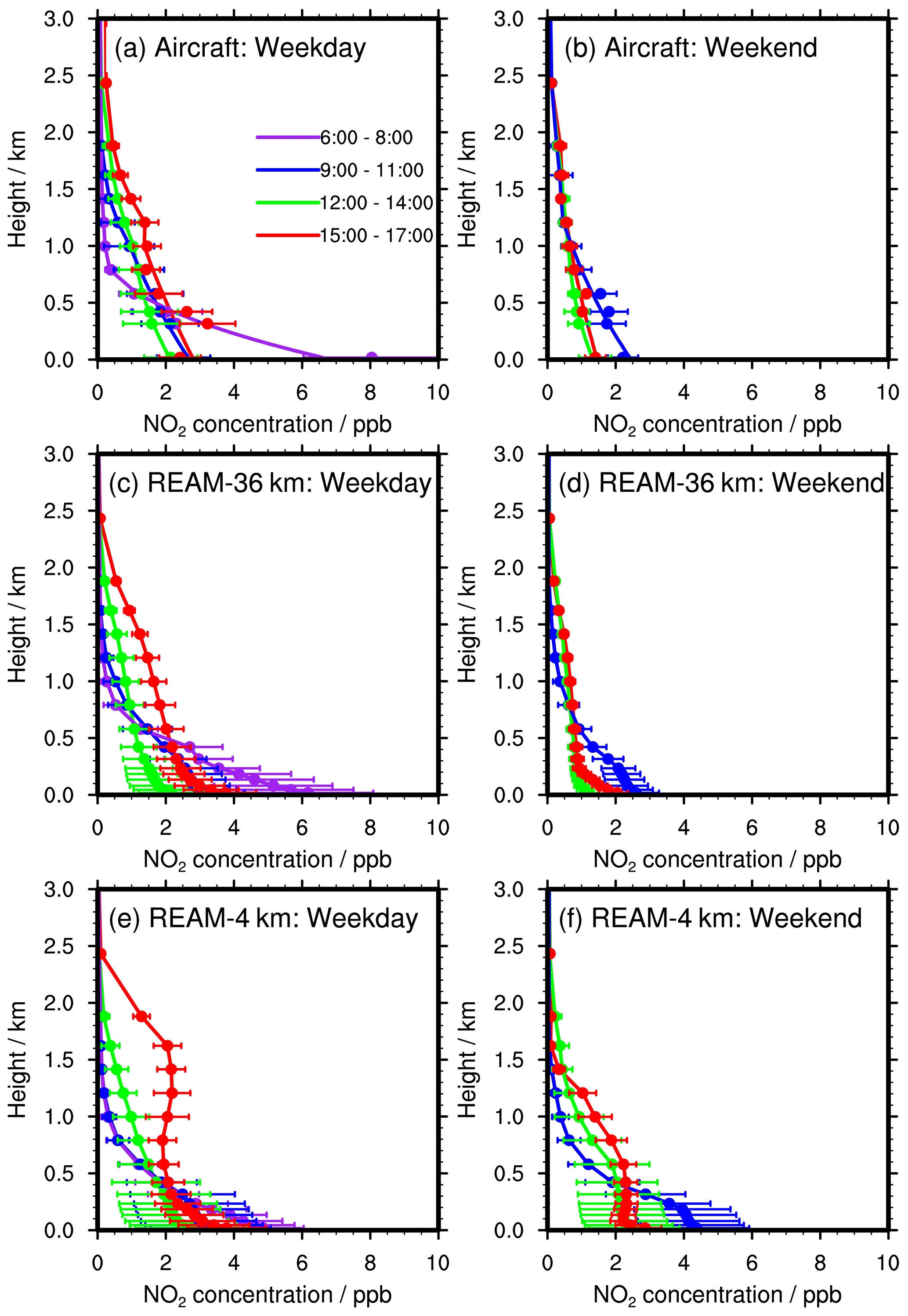
Figure 8 Temporal evolutions of NO₂ vertical profiles below 3 km on (a, c, e) weekdays and (b, d, f) weekends from the (a, b) P-3B aircraft and (c, d) 36 km and (e, f) 4 km REAM during the DISCOVER-AQ campaign. Horizontal bars denote the corresponding standard deviations. In (a, b), dots denote aircraft measurements, while lines below 1 km are based on quadratic polynomial fitting, as described in Sect. 2.6. The fitting values are mostly in reasonable agreement with the aircraft and surface measurements in the boundary layer. On weekends, no aircraft observations were made between 06:00 and 08:00 LT, and therefore no corresponding model profiles are shown.

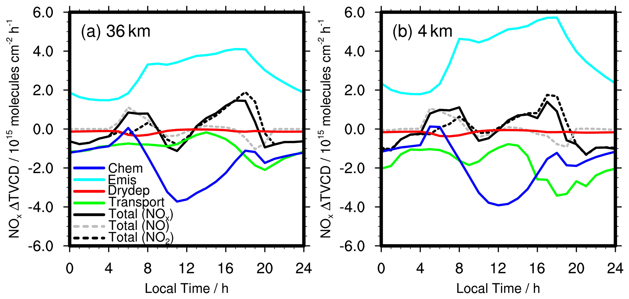
Figure 9 Contributions of emission, chemistry, transport, and dry deposition to NO_x TVCD diurnal variations over the 11 inland Pandora sites (Table S1 and Fig. 1) on weekdays in July 2011 for the (a) 36 km and (b) 4 km REAM simulations. “Chem” refers to net NO_x chemistry production; “Emis” refers to NO_x emissions; “Drydep” denotes NO_x dry depositions; “Transport” includes advection, turbulent mixing, lightning NO_x production, and wet deposition. “Total (NO_x)” is the hourly change in NO_x TVCDs ((TVCD) = TVCD_t+1 − TVCD_t). “Total (NO₂)” is the hourly change in NO₂ TVCDs, and “Total (NO)” is the hourly change in NO TVCDs.

3.3 Diurnal variations in NO₂ vertical profiles

Figure 8a and c show the temporal variations in P-3B-observed and 36 km REAM-simulated NO₂ vertical profiles in the daytime on weekdays during the DISCOVER-AQ campaign. The 36 km REAM reproduces the observed characteristics of NO₂ vertical profiles well in the daytime (R² = 0.89), which are strongly affected by vertical mixing and photochemistry (Y. Zhang et al., 2016). When vertical mixing is weak in the early morning (06:00–08:00 LT), NO₂, released mainly from surface NO_x sources, is concentrated in the surface layer, and the vertical gradient is large. As vertical mixing becomes stronger after 08:00 LT, NO₂ concentrations below 500 m decrease significantly, while those over 500 m increase from 06:00–08:00 to 12:00–14:00 LT. It is noteworthy that MLHs and NO_x emissions are comparable between 12:00–14:00 and 15:00–17:00 LT (Figs. 3 and 6); however, NO₂ concentrations between 15:00 and 17:00 LT are significantly higher than between 12:00 and 14:00 LT in the whole boundary layer, reflecting the impact of the decreased photochemical loss of NO_x in the late afternoon. In fact, photochemical losses affect all the daytime NO₂ vertical profiles, which can be easily identified by NO₂ TVCD process diagnostics discussed in Sect. 3.4 (Fig. 9).

Figure 8b and d also show the observed and 36 km REAM-simulated vertical profiles on weekends. Similar to Figs. 5 and 7, observed and simulated concentrations of NO₂ are lower on weekends than on weekdays. Some of the variations from weekend profiles are due to a lower number of observations (47 spirals) on weekends. The overall agreement between the observed vertical profiles and 36 km model results is good on weekends (R² = 0.87). Between 15:00 and 17:00 LT, the model simulates a larger gradient than what the combination of aircraft and surface measurements indicates. It may be related to the somewhat underestimated MLHs in the late afternoon in the model (Fig. 6).

On weekdays, most simulated vertical profiles at the 4 km resolution (Fig. 8e) are similar to 36 km results in part because the average NO_x emissions over the six P-3B spiral sites are about the same, 4 % lower in the 4 km than the 36 km REAM simulations (Table S1). A clear exception is the 4 km REAM-simulated vertical profile Between 15:00 and 17:00 LT when the model greatly overestimates boundary layer NO_x mixing and concentrations. The main reason is that WRF-simulated vertical velocities (W) in the late afternoon are much larger in the 4 km simulation than the 36 km simulation (Fig. S9), which can explain the simulated fully mixed boundary layer between 15:00 and 17:00 LT. Since it is not designed to run at the 4 km resolution, and it is commonly assumed that convection can be resolved explicitly at high resolutions, the Kain–Fritsch (new Eta) convection scheme is not used in the nested 4 km WRF simulation (Table S2); it may be related to the large vertical velocities in the late afternoon, when thermal instability is the strongest. Appropriate convection parameterization is likely still necessary for 4 km simulations (Zheng et al., 2016), which may also help alleviate the underestimation of precipitation in the nested 4 km WRF simulation as discussed in Sect. 3.1.

The same rapid boundary layer mixing due to vertical transport is present in the 4 km REAM-simulated weekend vertical profile (Fig. 8f), although the mixing height is lower. Fewer spirals (47) and distinct transport effect due to different NO₂ horizontal gradients between the 4 and 36 km REAM simulations (discussed in detail in Sect. 3.6) may cause the overestimation of weekend profiles in the 4 km REAM simulation.

3.4 Daytime variation in NO₂ TVCDs

We compare satellite, P-3B aircraft, and model-simulated TVCDs with Pandora measurements, which provide continuous daytime observations. The locations of Pandora sites are shown in Table S1 and Fig. 1. Among the Pandora sites, four sites are located significantly above the ground level: UMCP (∼ 20 m), UMBC (∼ 30 m), SERC (∼ 40 m), and GSFC (∼ 30 m). The other sites are 1.5 $\mathrm{m}\mathrm{a}.\mathrm{g}.\mathrm{l}.$ To properly compare Pandora to other measurements and model simulations, we calculate the missing TVCDs between the Pandora site heights and ground surface by multiplying the Pandora TVCDs with model-simulated TVCD fractions of the corresponding columns. The resulting correction is 2 %–21 % ($\frac{\mathrm{1}}{\mathrm{1}-\text{missing\hspace{0.17em} TVCD\hspace{0.17em} percentage}}$) for the four sites significantly above the ground surface, but the effect on the averaged daytime TVCD variation at all Pandora sites is small (Fig. S12). In the following analysis, we use the updated Pandora TVCD data.

Figure 10 Daily variations in NO₂ TVCDs on (a) weekdays and (b) weekends during the DISCOVER-AQ campaign. “REAM-36km” refers to the 36 km REAM simulation results over the 11 inland Pandora sites. “REAM-4 km” refers to the 4 km REAM simulation results over the 11 inland Pandora sites. “Pandora” refers to updated Pandora TVCD data. “Flight” denotes P-3B-aircraft-derived NO₂ VCDs below 3.63 km. “NASA-OMI” denotes the OMI NO₂ TVCDs retrieved by NASA over the Pandora sites; “KNMI-OMI” denotes the OMI NO₂ TVCDs from KNMI; “KNMI-GOME2” is the GOME-2A NO₂ TVCDs from KNMI. “OMI-retrieval” and “GOME2-retrieval” denote OMI and GOME-2A TVCDs retrieved by using the KNMI DOMINO algorithm with corresponding 36 km REAM vertical profiles, respectively. The vertical bars denote corresponding standard deviations for all data except the 36 km REAM simulation results, the standard deviations of which are shown with pink shading. We list NO₂ TVCD values at 09:30 and 13:30 LT in Table S3.

The weekday diurnal variations in NO₂ TVCDs from satellites, Pandora, 4 and 36 km REAM, and the P-3B aircraft are shown in Fig. 10a. We calculate aircraft-derived TVCDs by using Eq. (1):

$$\begin{array}{}\text{(1)}& {\mathrm{TVCD}}_{\mathrm{aircraft}}\left(t\right)={\displaystyle \frac{\sum c_{\text{aircraft}}\left(t\right)\cdot {\mathit{\rho }}_{\text{REAM}}\left(t\right)\cdot V_{\text{REAM}}\left(t\right)}{A_{\text{REAM}}}},\end{array}$$

where t is time, c_aircraft ($v/v$) denotes aircraft NO₂ concentrations (mixing ratios) at each level at time t, ρ_REAM (molecules cm⁻³) is the density of air from 36 km REAM at the corresponding level, V_REAM (cm³) is the volume of the corresponding 36 km REAM grid cell, and A_REAM (cm²) is the surface area (36 km × 36 km). In the calculation, we only use NO₂ concentrations below 3.63 $\mathrm{km}\mathrm{a}.\mathrm{g}.\mathrm{l}.$ because few aircraft measurements were available above this height in the campaign. Missing tropospheric NO₂ above 3.63 $\mathrm{km}\mathrm{a}.\mathrm{g}.\mathrm{l}.$ in the aircraft TVCD calculation has little impact on our analyses as the 36 km REAM model simulation shows that 85 % ± 7 % of tropospheric NO₂ is located below 3.63 $\mathrm{km}\mathrm{a}.\mathrm{g}.\mathrm{l}.$ between 06:00 and 17:00 LT in the DISCOVER-AQ region, which is roughly consistent with the GMI model results with 85 %–90 % tropospheric NO₂ concentrated below 5 km (Lamsal et al., 2014). It should be noted that only six P-3B spirals are available during the campaign, less than the samplings of 11 inland Pandora sites.

The 4 km REAM-simulated NO₂ TVCDs are mostly higher than the 36 km results and the observations in daytime on weekdays (Fig. 10a). However, since the standard deviations of the data are much larger than the model difference, the 4 and 36 km model results generally show similar characteristics relative to the observations. REAM simulation results are in reasonable agreement with Pandora, P-3B aircraft, and satellite daytime NO₂ TVCDs, except that NASA-derived OMI (OMNO2) TVCDs are somewhat lower than other datasets, which may be partly due to biased a priori vertical profiles from the GMI model in the NASA retrieval in the campaign (Lamsal et al., 2014, 2021). TVCDs derived by using the DOMINO algorithm and 36 km REAM NO₂ vertical profiles are in agreement with those from KNMI, which indicates that the TM4 model from KNMI provides reasonable estimates of a priori NO₂ vertical profiles on weekdays in the DISCOVER-AQ region in summer.

We find evident decreases in NO₂ TVCDs from GOME-2A to OMI in Fig. 10a, which is consistent with Pandora, REAM results, and previous studies that showed decreasing NO₂ TVCDs from SCIAMACHY to OMI due to photochemical losses in summer (Boersma et al., 2008, 2009). P-3B aircraft TVCDs also show this decrease feature but have large variations due in part to the limited aircraft sampling data.

Pandora NO₂ TVCD data have different characteristics from REAM-simulated and P-3B-aircraft-measured TVCDs between 05:00 and 07:00 and between 14:00 and 18:00 LT (Fig. 10a). Between 05:00 and 07:00 LT, Pandora data show a significant increase in NO₂ TVCDs, but REAM and aircraft TVCDs generally decrease, except for 4 km REAM TVCDs, with a slight increase from 06:00 to 07:00 LT on weekdays. Between 14:00 and 18:00 LT, Pandora TVCDs have little variation, but REAM and aircraft TVCDs increase significantly. The relatively flat Pandora TVCDs in the late afternoon compared to REAM and P-3B aircraft measurements are consistent with Lamsal et al. (2017), which found that Pandora VCDs were 26 %–30 % lower than UC-12 ACAM measurements from 16:00 to 18:00 LT during the DISCOVER-AQ campaign. We show the simulated effects of emission, chemistry, transport, and dry deposition on NO_x TVCDs in Fig. 9. The simulated early-morning slight decrease in NO₂ TVCDs is mainly due to the chemical transformation between NO₂ and NO favoring the accumulation of NO under low-O₃ and low-HO₂ and low-RO₂ conditions; thus NO TVCDs increase significantly, but NO₂ TVCDs continue decreasing slowly during the period. The increase in the late afternoon is primarily due to the decrease in photochemistry-related sinks. The reasons for the discrepancies of NO₂ TVCDs between Pandora and REAM results during the above two periods are unclear. Large SZAs in the early morning and the late afternoon (Fig. S1) lead to the higher uncertainties in Pandora measurements (Herman et al., 2009), although we have excluded Pandora measurements with SZA > 80^∘. In addition, Pandora is a sun-tracking instrument with a small effective FOV and is sensitive to local conditions within a narrow spatial range, which may differ significantly from the average properties of 36 and 4 km grid cells depending upon the time of the day (Fig. S13) (Herman et al., 2009, 2018, 2019; Judd et al., 2018, 2019, 2020; Lamsal et al., 2017; Reed et al., 2015). As we mentioned above, ∼ 85 % of tropospheric NO₂ is located below 3.63 km in the DISCOVER-AQ 2011 region based on the 36 km REAM simulation results. The Pandora FOV of 1.6^∘ is approximately equivalent to a nadir horizontal extension of only 0.1 km ($\mathrm{2}\times \mathrm{3.63}\mathrm{km}\times \tan \frac{\mathrm{1.6}}{\mathrm{2}}=\mathrm{0.1}$ km) at 3.63 $\mathrm{km}\mathrm{a}.\mathrm{g}.\mathrm{l}.$ and 30 m at 1.0 $\mathrm{km}\mathrm{a}.\mathrm{g}.\mathrm{l}.$ Therefore, Pandora measures different air columns of NO₂ at different times of the day, especially in the morning and afternoon, when SZA is large, as shown in Fig. S13. Considering the potential spatial heterogeneity of boundary layer NO₂, it is possible that the morning (east), noontime (nadir), and afternoon (west) NO₂ VCDs are significantly different from each other. Unlike Pandora, satellites and aircraft are far from the ground surface and cover large areas; therefore, the impact of SZA on their NO₂ VCD measurements is insignificant compared to Pandora measurements. Another possible reason is that Pandora instruments had few observations in the early morning, and the resulting average may not be representative (Fig. S2).

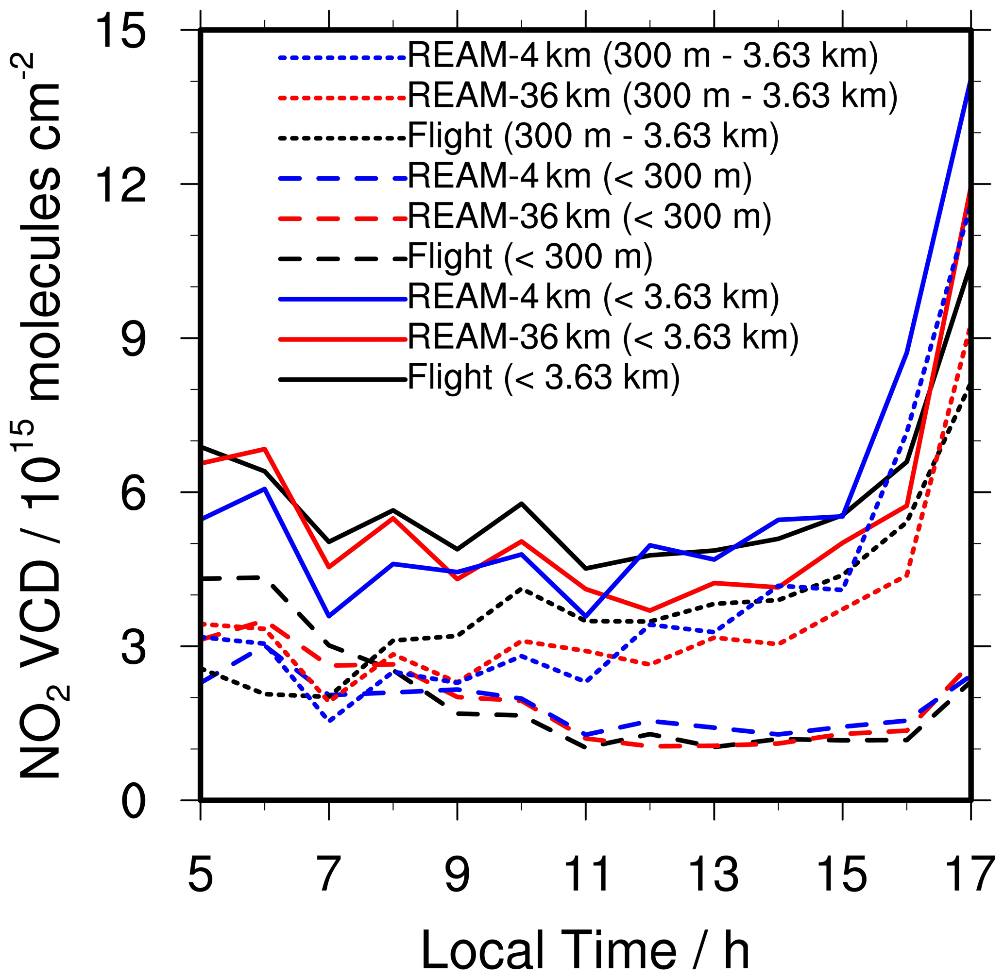
Figure 11 Weekday hourly variations in NO₂ VCDs at different height (a.g.l.) bins (< 3.63 $\mathrm{km}\mathrm{a}.\mathrm{g}.\mathrm{l}.$, < 300 $\mathrm{m}\mathrm{a}.\mathrm{g}.\mathrm{l}.$, and 300 m ∼ 3.63 $\mathrm{km}\mathrm{a}.\mathrm{g}.\mathrm{l}.$) based on P-3B-aircraft-derived datasets and the 36 and 4 km REAM results. “Flight” denotes P-3B-aircraft-derived NO₂ VCDs, “REAM-36km” denotes coincident 36 km REAM-simulated VCDs, and “REAM-4 km” denotes coincident 4 km REAM-simulated VCDs.

To further understand the daytime variation in NO₂ TVCDs, we examine P-3B-aircraft-data-derived and REAM-simulated NO₂ VCD variations for different height bins (Fig. 11). NO₂ VCDs below 3.63 $\mathrm{km}\mathrm{a}.\mathrm{g}.\mathrm{l}.$ display a U-shaped pattern from 05:00 to 17:00 LT. In the morning, as vertical mixing becomes stronger after sunrise, high-NO_x air in the lower layer is mixed with low-NO_x air in the upper layer. The increase in NO_x vertical mixing above 300 m is sufficient to counter the increase in photochemical loss in the morning. Conversely, the NO₂ VCDs below 300 m decrease remarkably from sunrise (about 06:00 LT) to around noontime due to both vertical mixing and the increase in photochemical strength. From 13:00 to 16:00 LT, NO₂ VCDs increase slowly, reflecting a relative balance among emissions, transport, chemistry, and dry depositions. The sharp jump of the VCDs from 16:00 to 17:00 LT is mainly due to dramatically reduced chemical loss. And 4 km REAM-simulated NO₂ VCDs at 0.30–3.63 km between 16:00 and 17:00 LT are much higher than 36 km results partly because of the rapid vertical mixing in the 4 km REAM simulation (Figs. 8 and S9).

Similar to NO₂ surface concentrations and vertical profiles in Figs. 7 and 8, the NO₂ TVCD variation is also smaller on weekends than on weekdays, but the day–night pattern is similar (Fig. 10). Although the 4 km REAM NO₂ TVCDs are generally higher than the 36 km results and observations in the daytime, considering their large standard deviations, NO₂ TVCDs from both simulations are comparable to satellite products, Pandora, and P-3B aircraft observations most of the time on weekends. The exception is that Pandora TVCDs have different variation patterns in the early morning and late afternoon from REAM simulations, similar to those found on weekdays.

3.5 Model comparisons with NO_y measurements

NO_y is longer-lived than NO_x, and NO_y concentrations are not affected by chemistry as much as NO_x. We obtain two types of NO_y concentrations from the P-3B aircraft in the DISCOVER-AQ campaign: one is NO_y concentrations directly measured by the NCAR four-channel instrument, corresponding to the sum of NO, NO₂, ∑PNs, ∑ANs, HNO₃, N₂O₅, HNO₄, HONO, and the other reactive nitrogenic species in REAM (all the other species are described in Table 1), and the other one, which we name “derived-NO_y”, is the sum of NO from the NCAR four-channel instrument and NO₂ (NO₂_LIF), ∑PNs, ∑ANs, and HNO₃ measured by the TD-LIF technique, corresponding to NO, NO₂, ∑PNs, ∑ANs, and HNO₃ in REAM (Table 1). On average, P-3B derived-NO_y concentrations (2.88 ± 2.24 ppb) are 17 % higher than coincident P-3B NO_y concentrations (2.46 ± 2.06 ppb), with R² = 0.75, generally reflecting consistency between these two types of measurements. As shown in Table 1, on weekdays, the 36 km REAM NO_y concentrations are 45 % larger than P-3B, with R² = 0.33, and the 36 km REAM derived-NO_y concentrations are 8 % larger than P-3B, with R² = 0.41. The 4 km REAM shows similar results, suggesting that REAM simulations generally reproduce the observed NO_y and derived-NO_y concentrations within the uncertainties, although the average values from REAM are somewhat larger than the observations due in part to the underestimate of precipitation in the WRF model simulations resulting in underestimated wet scavenging of HNO₃ in REAM. The concentrations of weekday NO, NO₂, and ∑PNs from REAM simulations are also comparable to the observations. However, weekday ∑ANs concentrations are 68 % lower in the 36 km REAM than observations, suggesting that the chemistry mechanism in REAM may need further improvement to better represent isoprene nitrates. It is noteworthy that, since ∑ANs only account for a small fraction (∼ 11 %) of observed derived-NO_y, the absolute difference between REAM-simulated and P-3B-observed ∑ANs concentrations is still small compared to HNO₃. Weekday HNO₃ concentrations are significantly higher in REAM simulations (36 km: 57 %, 0.65 ppb; 4 km: 74 %, 0.86 ppb) than P-3B observations, which is the main reason for the somewhat larger NO_y and derived-NO_y concentrations in REAM compared to P-3B observations. The higher HNO₃ concentrations in REAM may be related to the underestimation of precipitation in the corresponding WRF simulations, as discussed in Sect. 3.1 (Figs. S7 and S8), leading to the underestimated wet scavenging of HNO₃, especially for the 4 km REAM simulation.

We also examine the weekday diurnal variations in derived-NO_y vertical profiles from P-3B and REAM simulations in Fig. S14. Generally, both 36 and 4 km REAM simulations capture the variation characteristics of observed vertical profiles, which are similar to those for NO₂ in Fig. 8. REAM derived-NO_y concentrations are comparable to P-3B observations at most vertical levels on weekdays. Some larger derived-NO_y concentrations in the model results can be partially explained by larger HNO₃ concentrations in REAM, such as those below 1 km between 09:00 and 11:00 LT for the 36 km REAM and those below 2.0 km between 12:00 and 17:00 LT for the 4 km REAM (Fig. S15).

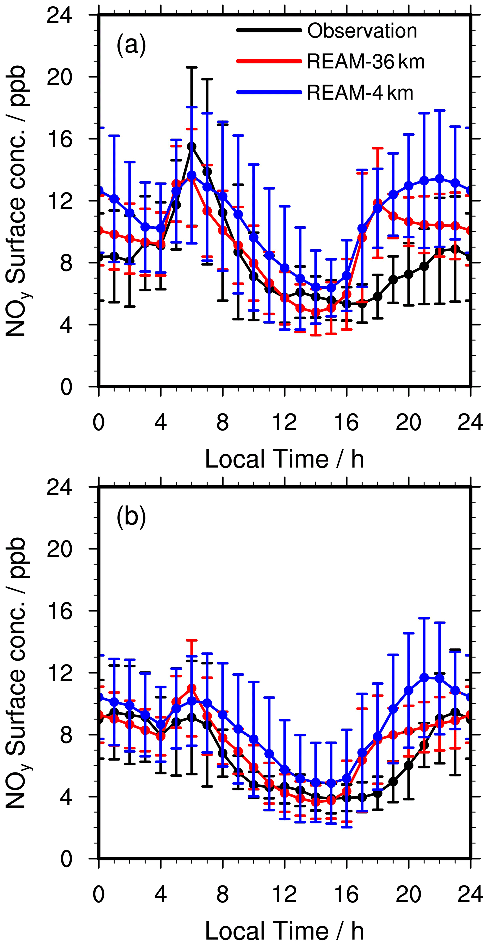
Figure 12 Diurnal cycles of observed and simulated average surface NO_y concentrations at Padonia, Edgewood, Beltsville, and Aldino on (a) weekdays and (b) weekends. Vertical bars denote the corresponding standard deviations. It is noteworthy that the mean NO_x emissions over Padonia, Edgewood, Beltsville, and Aldino are 99 % higher in the 4 than the 36 km REAM simulations (Table S1).

Figure 12 shows the comparison of the diurnal cycles of surface NO_y concentrations observed at Padonia, Edgewood, Beltsville, and Aldino during the DISCOVER-AQ campaign with those from the REAM simulations. Generally, the REAM simulations reproduce the observed surface NO_y diurnal cycles except for the spikes around 17:00–20:00 LT due to still-underestimated MLHs (Fig. 6). The 4 km simulation results have a higher bias than 36 km results relative to the observations in the daytime, similar to the comparisons of NO₂ surface concentrations and TVCDs in Figs. 7 and 10 due to higher emissions around the observation sites in 4 than 36 km simulations (Table S1 and Fig. 2).

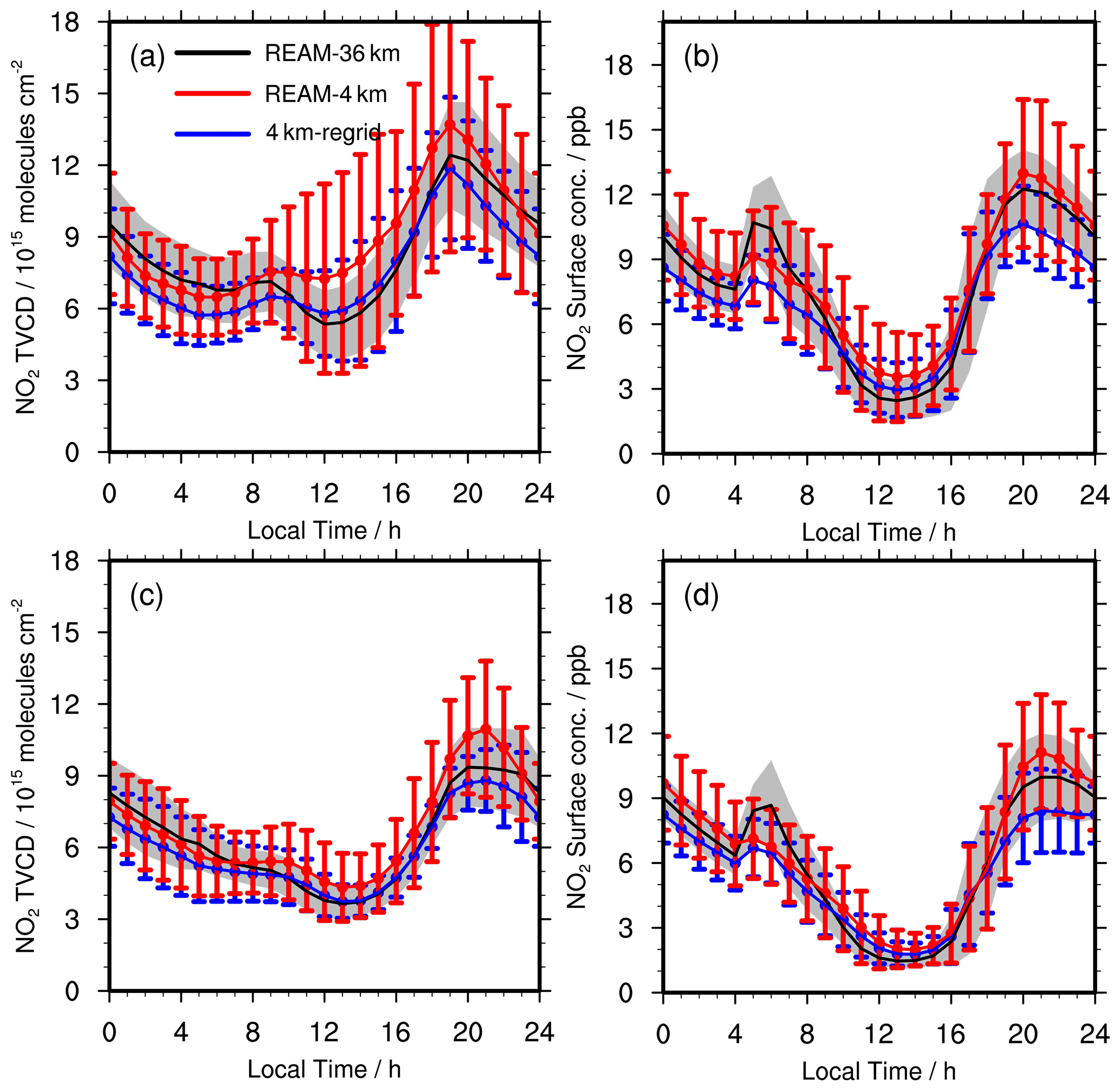
Figure 13 Comparisons of NO₂ (a, c) TVCDs and (b, d) surface concentrations over the 11 inland Pandora sites between the 4 and 36 km REAM simulations on (a, b) weekdays and (c, d) weekends for July 2011. “REAM-36km” (black lines) denotes the 36 km REAM simulation results; “REAM-4 km” (red lines) denotes the 4 km REAM simulation results; “4 km-regrid” (blue lines) refers to the 36 km values by regridding the 4 km REAM simulation results into 36 km REAM grid cells. The vertical bars denote corresponding standard deviations for all data except the 36 km REAM simulation results, the standard deviations of which are shown with gray shading.

Figure 14 Distributions of the scaled mean (a) 4 km REAM-simulated NO₂ VCDs below the UC-12 aircraft and (b) coincident ACAM measurements on weekdays in July 2011. (c) The distribution of the scaled NEI2011 NO_x emissions on weekdays. (d) The scatterplot of the scaled 4 km REAM and ACAM NO₂ VCDs from (a, b). Panel (e) shows the relative differences between (a) and (b) ($\text{REAM}/\text{ACAM}-\mathrm{1}$). (f) The distribution of the number of data points used to calculate grid cell mean NO₂ VCDs in (a, b). Here, we scale all values (VCDs and NO_x emissions) based on their corresponding domain averages. The domain averages of ACAM and coincident 4 km REAM NO₂ VCDs are 4.7 ± 2.0 and 4.6 ± 3.2 × 10¹⁵ molecules cm⁻², respectively.

3.6 Resolution dependence of NO_x emission distribution

We showed previously that the 4 km REAM-simulated NO₂ and NO_y surface concentrations and NO₂ TVCDs are higher than observations in the daytime in comparison to the corresponding 36 km REAM results (Figs. 7, 10, and 12). An examination of monthly mean NO₂ surface concentrations and TVCDs for July 2011 also shows that 4 km simulation results are significantly higher than the 36 km results over the 11 inland Pandora sites in the daytime (Fig. 13). The process-level diagnostics in Fig. 9 indicate that the mean contribution of NO_x emissions to NO_xΔTVCDs in the 4 km simulation is 1.32 × 10¹⁵ $\mathrm{molecules}{\mathrm{cm}}^{-\mathrm{2}}{\mathrm{h}}^{-\mathrm{1}}$ larger than that in the 36 km simulation between 09:00 and 16:00 LT, while the absolute mean contributions of chemistry and transport (they are negative in Fig. 9, so we use absolute values here) in the 4 km simulation are 0.26 × 10¹⁵ and 0.87 × 10¹⁵ $\mathrm{molecules}{\mathrm{cm}}^{-\mathrm{2}}{\mathrm{h}}^{-\mathrm{1}}$ larger than the 36 km simulation, respectively. The contributions of dry deposition to NO_xΔTVCDs are negligible compared to other factors in both simulations (Fig. 9). Therefore, the 34 % higher NO_x emissions over the 11 inland Pandora sites (Table S1 and Fig. 3) are the main reason for the larger daytime NO₂ surface concentrations and TVCDs in the 4 km than the 36 km REAM simulations (Fig. 13). The significantly different contribution changes between NO_x emissions (1.32 × 10¹⁵ $\mathrm{molecules}{\mathrm{cm}}^{-\mathrm{2}}{\mathrm{h}}^{-\mathrm{1}}$, or about one-third) and chemistry (0.26 × 10¹⁵ $\mathrm{molecules}{\mathrm{cm}}^{-\mathrm{2}}{\mathrm{h}}^{-\mathrm{1}}$, or about 8 %) reflect potential chemical nonlinearity (Li et al., 2019; Silvern et al., 2019; Valin et al., 2011) and transport effect. Different transport contributions between the 4 km and the 36 km REAM are mainly caused by their different NO_x horizontal gradients (Figs. 2, 14, and 15), while the impact of wind fields is small since we do not find significant differences in horizontal wind components between the two simulations except for some lower wind speeds below 1000 m for the 36 km WRF simulation compared to the nested 4 km WRF simulation (Fig. S16). Our sensitivity tests with the WRF single-moment three-class (WSM3) simple ice scheme (not shown) can improve the wind speed comparison below 1000 m between the 36 km and nested 4 km WRF simulations but still produce similar NO_x simulation results as WSM6 shown here. Therefore, the somewhat lower wind speeds below 1000 m in the 36 km WRF simulation are not the reason for the difference between the 4 and 36 km REAM simulations. The impact of transport on the two REAM simulations can be further verified by the comparison of NO₂ TVCDs over the six P-3B spiral sites between the two simulations (Fig. S17). Mean NO_x emissions over the six P-3B spiral sites are close (relative difference < 4 %) between the two simulations (Table S1 and Fig. S17). From 09:00 to 12:00 LT, the contributions of NO_x emissions to NO_xΔTVCDs are 2.50 × 10¹⁵ and 2.49 × 10¹⁵ $\mathrm{molecules}{\mathrm{cm}}^{-\mathrm{2}}{\mathrm{h}}^{-\mathrm{1}}$ for the 36 and 4 km REAM simulations, respectively, and the contributions of chemistry are also close between the two simulations (36 km: −2.62 × 10¹⁵ $\mathrm{molecules}{\mathrm{cm}}^{-\mathrm{2}}{\mathrm{h}}^{-\mathrm{1}}$; 4 km: −2.69 × 10¹⁵ $\mathrm{molecules}{\mathrm{cm}}^{-\mathrm{2}}{\mathrm{h}}^{-\mathrm{1}}$). However, the contributions of transport are −0.39 × 10¹⁵ and 0.03 × 10¹⁵ $\mathrm{molecules}{\mathrm{cm}}^{-\mathrm{2}}{\mathrm{h}}^{-\mathrm{1}}$ for the 36 and 4 km REAM simulations, respectively, leading to larger NO₂ TVCDs in the 4 km REAM simulation than the 36 km REAM from 09:00–12:00 LT (Fig. S17c). Since horizontal wind fields over the six P-3B spiral sites are comparable between two simulations (Figs. S4, S5, S6, and S16), and larger NO_x horizontal gradients are found near the P-3B spiral sites for the 4 km REAM (Fig. 2), we attribute the different transport contributions between the two simulations to a much larger NO_x emission gradient around the measurement locations in 4 than 36 km emission distributions.

We regrid the 4 km REAM results into the grid cells of the 36 km REAM, which can significantly reduce the impact of different NO_x emission distributions and associated transport on the two simulations. Compared to the original 4 km REAM results, the regridded surface NO₂ concentrations and TVCDs over the 11 inland Pandora sites are much closer to the 36 km REAM results (Fig. 13). After regridding the 4 km REAM results into 36 km REAM grid cells, we also find more comparable NO_y surface concentrations between the regridded 4 km results and the 36 km REAM results (Fig. S18). The remaining discrepancies between the regridded results and the 36 km REAM results may be due to chemical nonlinearity and other meteorological effects, such as larger vertical wind in the 4 km REAM (Fig. S9) and their different k_zz values in the PBL. Although other factors, such as chemical nonlinearity and vertical diffusion, may affect the 36 and 4 km REAM simulations differently, the difference between 4 and 36 km simulations of reactive nitrogen is largely due to that of NO_x emissions.

The 4 and 36 km simulation difference depends on the location of the observations. In some regions, the NO_x emission difference between 4 and 36 km simulations is small. The comparison of NO_y measurements from P-3B spirals with coincident REAM results in Table 1 suggests that the 4 and 36 km REAM simulations produce similar NO_y (relative difference ∼ 4 %) and derived-NO_y (relative difference ∼ 6 %) concentrations on weekdays, and both simulation results are comparable to the observations. The NO_y similarity over the P-3B spiral sites between the 36 and 4 km REAM simulations is consistent with the comparable NO_x emissions over (relative difference < 4 %) the six P-3B spiral sites between the two simulations (Table S1). The differences between the 4 km model simulation results and P3-B observations are larger on weekends than on weekdays (Table 1) due to the limited weekend sampling since model-simulated monthly mean values show similar differences between the 4 and 36 km REAM simulations on weekends as on weekdays (not shown).

3.7 Evaluation of 36 and 4 km NO_x distribution with OMI, GOME-2A, and ACAM measurements

The evaluation of model simulations of surface, aircraft, and satellite observations tends to point out a higher bias in 4 than 36 km model simulations. We note that this comparison is based on the averages of multiple sites. NO_x emissions at individual sites are not always higher in the 4 than 36 km REAM, such as SERC, Fairhill, and Essex, with much higher 36 km NO_x emissions than 4 km NO_x emissions (Table S1). We conduct individual-site comparisons of surface NO₂ concentrations, surface NO_y concentrations, NO₂ vertical profiles, derived-NO_y vertical profiles, and NO₂ TVCDs of the 36 km REAM and the 4 km REAM results relative to the corresponding observations in Figs. S19–S23. The 36 km simulation results can be larger, smaller, or comparable to the 4 km simulation results, and both simulations can produce higher, lower, or similar results as the observations for different variables at different sites. The varying model biases depending on the observation site reflect the different spatial distributions of NO_x emissions between the 36 and 4 km REAM simulations (Fig. 2) and suggest potential distribution biases of NO_x emissions in both simulations.

Here we examine the 4 km model-simulated NO₂ VCDs with high-resolution ACAM measurements onboard the UC-12 aircraft in Figs. 14 and S24, respectively. The spatial distributions of ACAM and 4 km REAM NO₂ VCDs are generally consistent with R² = 0.35 on weekdays and R² = 0.50 on weekends. The domain averages of ACAM and 4 km REAM NO₂ VCDs are 4.7 ± 2.0 and 4.6 ± 3.2 × 10¹⁵ molecules cm⁻² on weekdays and 3.0 ± 1.7 and 3.3 ± 2.7 × 10¹⁵ molecules cm⁻² on weekends, respectively. The spatial distributions of ACAM and 4 km REAM NO₂ VCDs are highly correlated with the spatial distribution of 4 km NEI2011 NO_x emissions. All three distributions capture two strong peaks around Baltimore and Washington, DC, urban regions and another weak peak in the northeast corner of the domain (Wilmington, Delaware) (Figs. 14 and S24). However, Figs. 14 and S24 clearly show that NO₂ VCDs from the 4 km REAM simulation are more concentrated in Baltimore and Washington, DC, urban regions than ACAM, which are also reflected by the higher NO₂ VCD standard deviations of the 4 km REAM results than ACAM. Several Pandora sites are in the highest NO₂ VCD regions, where the 4 km REAM generally produces larger NO₂ VCDs than ACAM, which explains why the NO₂ TVCDs over the 11 Pandora sites from the 4 km REAM simulation are higher than the observations (Fig. 10) and the 36 km REAM results (Fig. 13) around noontime. Horizontal transport cannot explain the NO₂ VCD distribution biases in the 4 km REAM simulation due to the following reasons. Firstly, horizontal wind fields are simulated as well by the nested 4 km WRF simulation as the 36 km WRF compared to P-3B measurements, as discussed in Sect. 3.1. Secondly, the prevailing northwest wind in the daytime (Fig. S5) should move NO_x eastward, but we find no significant eastward shift in NO₂ VCDs compared to NO_x emissions in both ACAM and 4 km REAM distributions (Fig. 14). Therefore, we attribute the distribution inconsistency between ACAM and the 4 km REAM to the distribution biases of NEI2011 NO_x emissions at the 4 km resolution since the average below-aircraft NO₂ VCDs between ACAM and the 4 km REAM are about the same.

It is noteworthy that the number of data points used to calculate grid cell mean NO₂ VCDs varies significantly across the domain, as shown in Figs. 14f and S24f. To mitigate potential sampling errors, we only consider the grid cells with ≥ 10 data points on weekdays in Fig. S25. Whether we scale NO₂ VCDs using the corresponding domain averages (Fig. S25) or not (not shown), the 4 km REAM generally shows more concentrated NO₂ VCDs in Baltimore and Washington, DC, urban regions but more dispersed NO₂ VCDs in rural areas than ACAM, consistent with our discussion above. In addition, about 91 % of ACAM NO₂ VCD data are measured from 08:00–16:00 LT, and only using ACAM NO₂ VCDs between 08:00 and 16:00 LT for the above comparison does not affect our results shown here. Moreover, to minimize the effect of overestimated afternoon vertical mixing (Fig. 8) on the 4 km REAM simulation results, we also examine the comparison between ACAM NO₂ VCDs from 09:00–14:00 LT with coincident 4 km REAM results, which produces similar results as shown here. Finally, considering the NO_x lifetime difference between morning and noontime, we also analyze the NO₂ VCD data between 11:00 and 14:00 LT, and similar results are found.

We also evaluate the NO₂ VCD distributions from the 4 km REAM simulation on weekdays and weekends with ACAM NO₂ VCDs below the U-12 aircraft obtained from https://www-air.larc.nasa.gov/cgi-bin/ArcView/discover-aq.dc-2011?UC12=1#LIU.XIONG/ (last access: 31 December 2019) in Figs. S26 and S27. Although the domain mean ACAM NO₂ VCDs in Figs. S26 and S27 are higher than coincident 4 km REAM results due to the different retrieval method from Lamsal et al. (2017), such as different above-aircraft NO₂ VCDs and different a priori NO₂ vertical profiles, we can still find clear distribution inconsistencies between the 4 km REAM and ACAM NO₂ VCDs. The 4 km REAM NO₂ VCDs are more concentrated in the Baltimore and Washington, DC, urban regions than this set of ACAM data, which is consistent with the conclusions derived from the ACAM dataset retrieved by Lamsal et al. (2017).

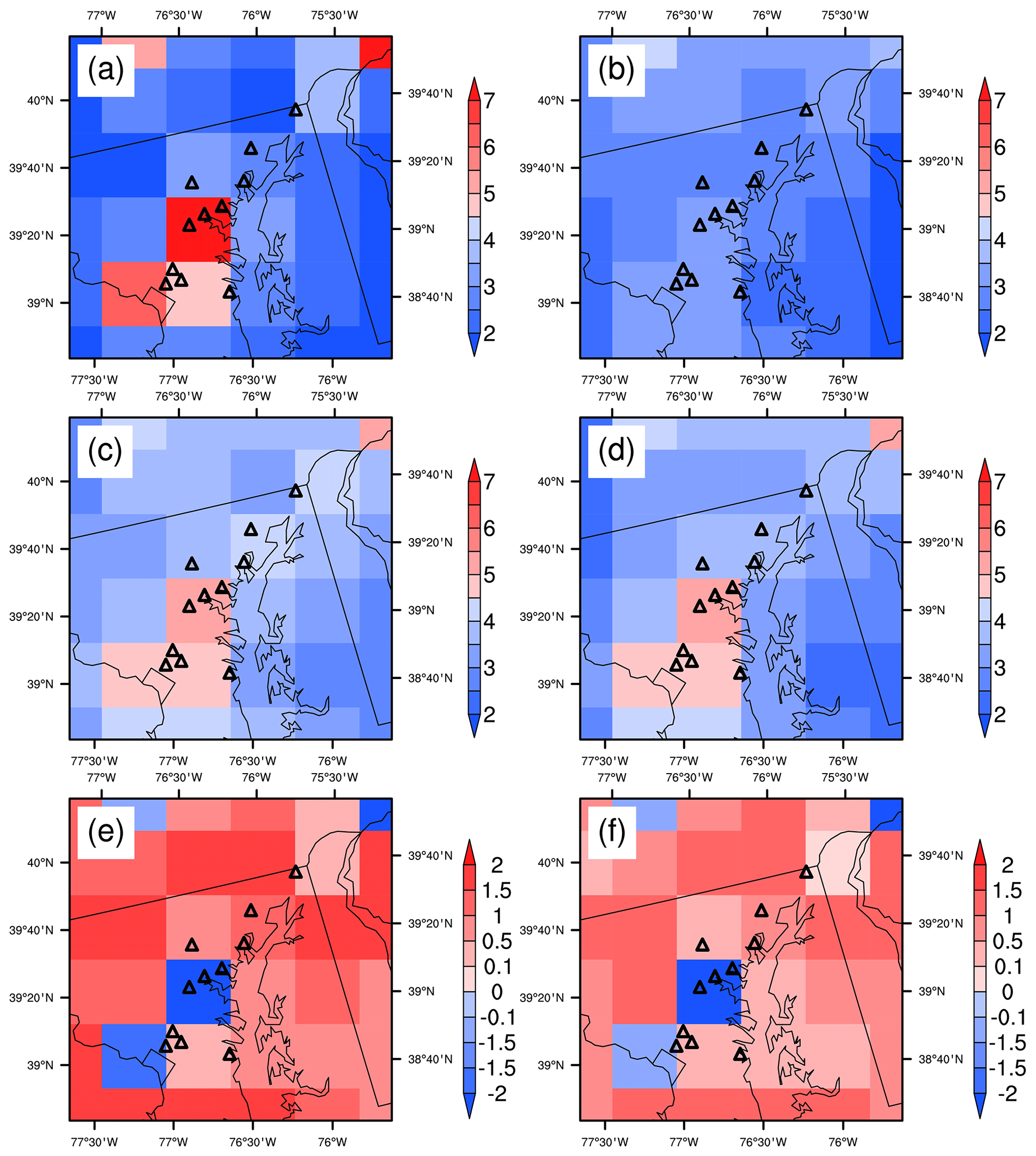
Figure 15 Distributions of weekday NO₂ TVCDs around the DISCOVER-AQ 2011 region for 13:30 LT in July 2011: (a) the 36 km REAM simulation results, (b) the NASA OMI product (OMNO2), (c) the KNMI OMI product, (d) the retrieved OMI NO₂ TVCDs by using the KNMI DOMINO algorithm with corresponding 36 km REAM vertical profiles, (e) the distribution of the NO₂ TVCD differences (c minus a) between KNMI OMI and 36 km REAM, and (f) the difference (d minus a) between retrieved OMI NO₂ TVCDs and the 36 km REAM results. The NO₂ TVCD unit is 10¹⁵ molecules cm⁻².

The potential distribution bias of the NEI2011 NO_x emissions at 36 km resolution is analyzed by comparing the 36 km REAM-simulated NO₂ TVCDs with those retrieved by OMI and GOME-2A, as shown in Figs. 15 (OMI, 13:00 LT) and S28 (GOME-2A, 09:30 LT). Both KNMI and our retrievals based on the 36 km REAM NO₂ vertical profiles show that OMI and GOME-2A NO₂ TVCDs have lower spatial variations than the corresponding 36 km REAM simulation results. OMI and GOME-2A retrievals have lower NO₂ TVCDs around the Baltimore and Washington, DC, urban regions and higher values in relatively rural regions than the 36 km REAM. The distribution bias of the 36 km REAM NO₂ TVCDs is also identified on weekends through their comparison with OMI and GOME-2A retrievals (not shown). The good agreement between simulated and observed wind suggests that the model horizontal transport error cannot explain such an urban–rural contrast between satellite observations and 36 km REAM simulation results. However, two caveats deserve attention. Firstly, the 36 km REAM cannot resolve urban areas as detailed as the 4 km REAM (Fig. 14), and urban and rural regions may coexist in one 36 km grid cell. Secondly, the OMI and GOME-2A pixels can be much larger than 36 km REAM grid cells, possibly leading to more spatially homogenous distributions of satellite NO₂ TVCD data.

3.8 Implications for NO_x emissions

The analysis of Sect. 3.7 indicates that the NEI2011 NO_x emission distributions at 36 and 4 km resolutions are likely biased for the Baltimore–Washington region. The distribution bias of NO_x emission inventories is corroborated by the comparison of the NO_x emission inventory derived from the CONsolidated Community Emissions Processor Tool, Motor Vehicle (CONCEPT MV) v2.1 with that estimated by the Sparse Matrix Operator Kernel Emissions (SMOKE) v3.0 model with the Motor Vehicle Emissions Simulator (MOVES) v2010a (DenBleyker et al., 2012). CONCEPT, with finer vehicle activity information as input, produced wider-spread but less-concentrated running exhaust NO_x emissions compared to MOVES in the Denver urban area for July 2008 (DenBleyker et al., 2012). In addition, Canty et al. (2015) found that CMAQ 4.7.1, with on-road emissions from MOVES and off-road emissions from the National Mobile Inventory Model (NMIM), overestimated NO₂ TVCD over urban regions and underestimated NO₂ TVCDs over rural areas in the northeastern US for July and August 2011 compared to the OMNO2 product. The urban–rural contrast was also found in Texas during the 2013 DISCOVER-AQ campaign in the studies of Souri et al. (2016, 2018), implying distribution uncertainties in NO_x emissions, although these studies and Canty et al. (2015) focused more on polluted regions with overestimated NO_x emissions in their conclusions. The emission distribution bias may also explain why Anderson et al. (2014) have different results from our simulated concentrations in Table 1. In their study, they compared in situ observations with a nested CMAQ simulation with a resolution of 1.33 km. It is difficult to build up a reliable emission inventory for the whole US at very high resolutions with currently available datasets due to the significant inhomogeneity of NO_x emissions (Marr et al., 2013), but we can still expect significant improvements in the temporal-spatial distributions of NO_x emissions in the near future as GPS-based information starts to be used in the National Emissions Inventory (NEI) estimates (DenBleyker et al., 2017).

Here, we emphasize that our study is not necessarily contradictory to recent studies concerning the overestimation of NEI NO_x emissions (Anderson et al., 2014; Canty et al., 2015; McDonald et al., 2018; Souri et al., 2016, 2018; Travis et al., 2016). Different types of observations in different periods and locations are analyzed for various purposes. This study focuses more on the spatial distribution of NO_x emissions in NEI2011, while previous studies are concerned more about the NO_x emission magnitudes in highly polluted sites, although the spatial distribution issue was also mentioned in some of the studies. If we limit our analyses to those observations in Figs. 7, 10, and 12 and the 4 km REAM, we would also conclude an overestimation of NEI NO_x emissions. Considering the significant heterogeneity of NO_x emissions, the spatial distribution of NO_x emissions is a critical factor in evaluating NO_x emissions and improving emission estimation and air quality models, which deserves more attention in future studies, especially when chemical and transport models are moving to higher and higher resolutions.

4 Conclusions

We investigate the diurnal cycles of surface NO₂ concentrations, NO₂ vertical profiles, and NO₂ TVCDs using REAM model simulations on the basis of the observations from air quality monitoring sites, aircraft, Pandora, OMI, and GOME-2A during the DISCOVER-AQ 2011 campaign. We find that WRF-simulated nighttime k_zz-determined MLHs are significantly lower than ELF lidar measurements. Increasing nighttime mixing from 18:00–05:00 LT in the REAM simulations, we significantly improve REAM simulations of nighttime surface NO₂ and O₃ concentrations.

The REAM simulation reproduces the observed regional mean diurnal cycles of surface NO₂ and NO_y concentrations, NO₂ vertical profiles, and NO₂ TVCDs well on weekdays. Observed NO₂ concentrations in the boundary layer and TVCDs on weekends are significantly lower than on weekdays. By specifying a weekend-to-weekday NO_x emission ratio of $\mathrm{2}/\mathrm{3}$ and applying a less variable NO_x emission diurnal profile on weekends than weekdays, REAM can simulate the weekend observations well. Two issues are also noted. First, Pandora TVCDs show different variations from aircraft-derived and REAM-simulated TVCDs in the early morning and late afternoon, which may be due to the uncertainties in Pandora measurements at large SZAs and the small effective FOV of Pandora. Second, the weekday OMI NO₂ TVCDs derived by NASA are somewhat lower than the KNMI OMI product, P-3B-aircraft-derived TVCDs, Pandora, and REAM results; the difference may be caused by the a priori vertical profiles used in the NASA retrieval.

While a higher-resolution simulation is assumed to be superior at a priori, the large observation dataset during DISCOVER-AQ 2011 offers the opportunity of a detailed comparison of 4 and 36 km model simulations. Through the comparison, we find two areas that have not been widely recognized. The first is not using convection parameterization in high-resolution WRF simulations since convection can be resolved explicitly, and most convection parameterizations are not designed for high-resolution simulations. We find that 4 km WRF tends to overestimate boundary layer mixing and vertical transport in the late afternoon, leading to a high model bias in simulated NO₂ vertical profiles compared to P-3B aircraft observations. The reasons for this late-afternoon bias in 4 km WRF simulations and model modifications to mitigate this bias need further studies.

A second issue is related to the spatial distribution of NO_x emissions in NEI2011. In general, the 4 km simulation results tend to have a high bias relative to the 36 km results on the regional mean observations. However, for individual sites, relative to the 36 km model simulations, the 4 km model results can show larger, smaller, or similar biases compared to the observations depending upon observation location. Based on process diagnostics and analyses, we find that the bias discrepancies between the 36 and 4 km REAM simulations are mainly attributed to their different NO_x emissions and their spatial gradients at different sites. The comparison of 4 km ACAM NO₂ VCD measurements from the UC-12 aircraft with coincident 4 km REAM results shows that 4 km REAM NO₂ VCDs are more concentrated in urban regions than the ACAM observations. OMI and GOME-2A data also show less spatially varying NO₂ TVCD distributions with lower NO₂ TVCDs around the Baltimore–Washington urban regions and higher TVCDs in surrounding rural areas than corresponding 36 km REAM simulation results. Further model analysis indicates that the 36 and 4 km VCD discrepancies are due primarily to the distribution bias of NEI2011 NO_x emissions at 36 and 4 km resolutions. Our results highlight the research need to improve the methodologies and datasets to improve the spatial distributions in emission estimates.