Impact of stratospheric air and surface emissions on tropospheric nitrous oxide during ATom

We measured the global distribution of tropospheric N₂O mixing ratios during the NASA airborne Atmospheric Tomography (ATom) mission. ATom measured concentrations of ∼ 300 gas species and aerosol properties in 647 vertical profiles spanning the Pacific, Atlantic, Arctic, and much of the Southern Ocean basins, nearly from pole to pole, over four seasons (2016–2018). We measured N₂O concentrations at 1 Hz using a quantum cascade laser spectrometer (QCLS). We introduced a new spectral retrieval method to account for the pressure and temperature sensitivity of the instrument when deployed on aircraft. This retrieval strategy improved the precision of our ATom QCLS N₂O measurements by a factor of three (based on the standard deviation of calibration measurements). Our measurements show that most of the variance of N₂O mixing ratios in the troposphere is driven by the influence of N₂O-depleted stratospheric air, especially at mid- and high latitudes. We observe the downward propagation of lower N₂O mixing ratios (compared to surface stations) that tracks the influence of stratosphere–troposphere exchange through the tropospheric column down to the surface. The highest N₂O mixing ratios occur close to the Equator, extending through the boundary layer and free troposphere. We observed influences from a complex and diverse mixture of N₂O sources, with emission source types identified using the rich suite of chemical species measured on ATom and the geographical origin calculated using an atmospheric transport model. Although ATom flights were mostly over the oceans, the most prominent N₂O enhancements were associated with anthropogenic emissions, including from industry (e.g., oil and gas), urban sources, and biomass burning, especially in the tropical Atlantic outflow from Africa. Enhanced N₂O mixing ratios are mostly associated with pollution-related tracers arriving from the coastal area of Nigeria. Peaks of N₂O are often associated with indicators of photochemical processing, suggesting possible unexpected source processes. In most cases, the results show how difficult it is to separate the mixture of different sources in the atmosphere, which may contribute to uncertainties in the N₂O global budget. The extensive data set from ATom will help improve the understanding of N₂O emission processes and their representation in global models.

1 Introduction

Nitrous oxide (N₂O) is a powerful greenhouse gas and, due to its oxidation to NO_x, a major contributor to both stratospheric ozone loss and to the passivation of stratospheric oxy-halogen radicals (Forster et al., 2007; Ravishankara et al., 2009). The rate of increase in atmospheric N₂O since the Industrial Revolution, 0.93 ppb yr⁻¹, implies a significant (∼ 30 %) imbalance between emission rates and destruction in the stratosphere. Seasonal cycles in tropospheric N₂O are driven by both stratosphere-to-troposphere exchange and surface emissions (Nevison et al., 2011; Assonov et al., 2013; Thompson et al., 2014a). Most N₂O emissions are attributed to microbial nitrification and denitrification in natural and cultivated soils, freshwaters, and oceans plus emissions related to human activities, such as biomass burning and industrial emissions (Butterbach-Bahl et al., 2013; Saikawa et al., 2014; Thompson et al., 2014a; Upstill-Goddard et al., 2017; WMO, 2018).

Much effort has been made to reduce the uncertainties in the individual components of the N₂O global budget (e.g., Tian et al., 2012, 2020; Xiang et al., 2013; Thompson et al., 2014a, b; Ganesan et al., 2020; Yang et al., 2020). Recent estimates of global total N₂O emissions to the atmosphere from bottom-up and top-down methods average 17 Tg N yr⁻¹ (12.2–23.5 from bottom-up analysis and 15.9–17.7 Tg N yr⁻¹ from top-down approaches, Tian et al., 2020). The most recent estimates of the global ocean emissions of N₂O range between 2.5 and 4.3 Tg N yr⁻¹ (∼ 20 % of total emissions), with the tropics, upwelling coastal areas, and subpolar regions the major contributors to these fluxes (Yang et al., 2020; Tian et al., 2020). However, the magnitude of marine N₂O emissions is subject to large uncertainty due to spatial and temporal heterogeneity (Nevison et al., 1995, 2005; Ganesan et al., 2020; Yang et al., 2020). According to Tian et al. (2020), anthropogenic sources account for ∼ 43 % of global N₂O emissions (7.3 Tg N yr⁻¹), with industry and biomass burning emissions estimated to be 1.6–1.9 Tg N yr⁻¹, respectively (Syakila and Kroeze, 2011; Tian et al., 2020) and the rest originating from agriculture. N₂O emissions from biogenic sources and fires in Africa are estimated at 3.3 ± 1.3 Tg N₂O yr⁻¹ (Valentini et al., 2014). Agricultural N₂O emission estimates (up to ∼ 37 %) range between 2.5 and 5.8 Tg N yr⁻¹, and between 4.9 and 6.5 Tg N yr⁻¹ in the case of natural soils (Kort et al., 2008, 2010; Syakila and Kroeze, 2011; Tian et al., 2020). Recent estimates of N₂O emissions from fertilized tropical and subtropical agricultural systems are 3 ± 5 kg N ha⁻¹ yr⁻¹ (Albanito et al., 2017). Most of these estimates are derived from short-term local-scale in-situ measurements and are difficult to extrapolate with confidence to large regions or to the globe.

In the atmosphere, N₂O is destroyed by oxidation (10 %, O(¹D) reaction) and photolysis (90 %, 190–230 nm photolysis) in the upper stratosphere (> 20 km altitude; SPARC, 2013), which makes it a good candidate for tracing the air exchange between the stratosphere and the troposphere (Hintsa et al., 1998; Nevison et al., 2011; Assonov et al., 2013; Krause et al., 2018). Atmospheric models tend to underestimate the interhemispheric N₂O gradient, which Thompson et al. (2014a) attribute to an overestimation of N₂O emissions in the Southern Ocean, an underestimate of Northern Hemisphere emissions, and/or an overestimate of stratosphere-to-troposphere exchange in the Northern Hemisphere. Overall, the largest uncertainties in modeled N₂O emissions are found in tropical South America and South Asia (Thompson et al., 2014b).

We present atmospheric N₂O altitude profiles at high temporal resolution collected during the NASA Atmospheric Tomography (ATom) mission. ATom was a global-scale airborne deployment conducted over a 3 year period (2016–2018) using the NASA DC-8 aircraft. In ATom, the DC-8 flew vertical profiles (0.2–13 km) nearly continuously almost from pole to pole while measuring mixing ratios of ∼ 300 trace gases and aerosol physical and chemical properties over the Pacific and Atlantic basins and during each of the four seasons. Each deployment (1–4) started and ended in Palmdale (California, USA) and generally consisted of a loop southward from the Arctic through the central Pacific, across the Southern Ocean to South America, northward through the Atlantic, and across Greenland and the Arctic Ocean. During ATom-3 and -4, two additional flights from Punta Arenas (Chile) sampled the Antarctic troposphere and upper troposphere/lower stratosphere (UT/LS) to 80^∘ S.

In this work, we focus on the measurements taken during January–February 2017 (ATom-2), September–October 2017 (ATom-3), and April–May 2018 (ATom-4) (no quantum cascade laser spectrometer (QCLS) N₂O data are available for ATom-1 in August 2016). The motivation for this paper is twofold. Firstly, we present a new retrieval strategy to account for the pressure and temperature dependence of laser-based instruments, and specifically for the use of quantum cascade laser spectrometers on aircraft. Secondly, we report on the global distribution of N₂O from the surface to 13 km and examine the processes contributing to the variability of tropospheric N₂O based on the vertical profiles of N₂O and a broad variety of covariate chemical species and aerosol properties.

2 Instrument specifications, spectral analysis, and calibration

2.1 Specifications of QCLS

We measured N₂O mixing ratios with the Harvard/NCAR/Aerodyne Research Inc. Quantum Cascade Laser Spectrometer (QCLS). This instrument was previously deployed on the NCAR/NSF Gulfstream V for the HIAPER Pole-to-Pole Observations mission (HIPPO, Wofsy et al., 2011; https://www.eol.ucar.edu/field_projects/hippo, last access: 14 October 2020) and the O₂ $/$ N₂ Ratio and CO₂ Southern Ocean Study (ORCAS, Stephens et al., 2018; https://www.eol.ucar.edu/field_projects/orcas, last access: 14 October 2020). Detailed information about the spectrometer configuration can be found in Jiménez et al. (2005, 2006) and Santoni et al. (2014). A brief description follows.

QCLS provides continuous (1 Hz) measurements of N₂O, methane (CH₄), and carbon monoxide (CO) using two thermoelectrically cooled pulsed quantum cascade lasers, a 76 m pathlength multiple-pass absorption cell (∼ 0.5 L volume), and two liquid-nitrogen-cooled solid-state HgCdTe detectors. All these components are mounted on a temperature-stabilized, vibrationally isolated optical bench. The temperature in QCLS is controlled by Peltier elements coupled with a closed-circuit recirculating fluid kept at 288.0 ± 0.1 K. QCLS measures CH₄ and N₂O by scanning the spectral interval of 1275.45 ± 0.15 cm⁻¹. A second laser is used to scan CO at 2169.15 ± 0.15 cm⁻¹. The supply currents to QCLS are ramped at a rate of 3.8 kHz to scan the laser frequency for 200 channels (steps in frequency) in laser 1 and 50 channels in laser 2; an extra 10 channels are used to measure the laser shut off (zero-light level). The spectra and fit residuals for CH₄, N₂O, and CO are shown in Fig. S1 of the Supplement. Mixing ratios are derived at a rate of 1 Hz by a least-squares spectral fit assuming a Voigt line profile at the pressure and temperature measured inside the sample cell and using molecular line parameters from the HIgh-resolution TRANsmission molecular absorption database (HITRAN, Rothman et al., 2005). The temperature and pressure inside the cell are monitored with a 30 kΩ thermistor and a capacitance manometer (133 hPa full scale), respectively.

During sampling, the air passes through a 50-tube Nafion drier to remove the bulk water vapor. A Teflon diaphragm pump downstream of the cell reduces the air pressure to ∼ 60 hPa. Both ambient air and calibration gases pass through a Teflon dry-ice trap to reduce the dew point to −70 ^∘C. After ATom-1, we added a bypass between the inlet and the instrument to increase the flushing rate of the inlet and inlet tubing. The calibration sequence includes 2 min of ultra-high-purity zero air followed by 1 min each of low- and high-mixing ratio gases every 30 min (see Fig. S2). We measured zero air every 15 min during ATom-1 and -2, and every 30 min during ATom-3 and -4. A data logger (CR10X, Campbell Scientific) was used to automate the sampling sequence. The CR10X controlled the pressure controller on the cell and managed the data transfer.

We use gas cylinders traceable to the National Oceanic and Atmospheric Administration World Meteorological Organization scales for calibration (NOAA-WMO-X2004A scale for CH₄, WMO-X2014A for CO, and NOAA-2006A for N₂O). These gas standards were recalibrated before, during and after the deployments to maintain traceability. The low mixing ratio gas cylinder contained 298.5 ± 0.3 ppb of N₂O, 1692.4 ± 0.2 ppb of CH₄, and 119.1 ± 0.3 ppb of CO. The high mixing ratio gas cylinder contained 399.1 ± 0.3 ppb of N₂O, 2182.5 ± 0.3 ppb of CH₄, and 192.8 ± 0.5 ppb of CO. Detailed information on calibrations of the gas cylinders used during ATom is given in Table S1 of the Supplement.

QCLS also measures carbon dioxide (CO₂) in a separate unit. Detailed information about QCLS CO₂ measurements can be found in Santoni et al. (2014).

2.2 Spectral analysis and calibration

QCLS was damaged during shipping to the deployment site before the start of ATom-1, and the resulting alteration in the optical alignment modified the sensitivity of the instrument to temperature and pressure changes during aircraft maneuvers. This increased sensitivity was observed in all ATom deployments. At constant altitude, instrumental precision was similar to the precision measured during HIPPO (see the Allan–Werle variance analysis in Fig. 2 in Santoni et al., 2014 for HIPPO and Fig. S3 for ATom), but drifts were observed during altitude changes due to the effects of changes in cabin pressure and temperature on the spectral location of interference fringes that arise in the optical path outside the sample cell. In addition, flight altitude changes mechanically stressed the optical elements surrounding the cell, further modulating fringes or changing the shape of the detected laser intensity profile. These spectral artifacts ultimately reduced the accuracy of mixing ratios retrieved from spectral fitting. The spectral artifacts most strongly affected the measurements of CH₄ and N₂O. Several post-processing methods using the TDL-Wintel software were explored to improve the precision and accuracy of ATom QCLS N₂O data, most with little success. Since the measured spectra were all saved, it is possible to refit the data with different fit parameters. A limited number of interference fringes may be included in the set of fitting functions. However, none of the previously used full refitting strategies significantly improved the data accuracy.

We have achieved significant improvements in the precision and accuracy of the ATom QCLS N₂O data using a new method dubbed the “Neptune algorithm,” developed by Aerodyne Research, Inc., and that method has been further developed and applied to the data sets described here. Using this algorithm, the precision of the retrieved N₂O data measured with the damaged QCLS was similar to that reported in HIPPO. The Neptune algorithm generates corrections to the mixing ratios retrieved from the original fits by associating specific spectral features with anomalies in retrieved mixing ratios observed during calibrations, i.e., during intervals when the mixing ratios are held constant. The spectral baseline is defined as the spectral channels outside the boundaries of the spectral lines of the target gas. Fluctuations in the spectral baselines are quantified for the entire data set by means of principal component analysis (PCA). PCA provides an efficient description of the spectral fluctuations, naturally producing an ordered set from the strongest to the weakest orthogonal vectors (spectral forms), each with an amplitude history spanning the data set. The PCAs are defined by an optimization procedure during calibrations, when mixing ratio fluctuations are designed to be ∼ 0. The finite fluctuations in retrieved mixing ratios during calibrations are fitted in the spectral space of the baseline as linear combinations of the leading PCA vector amplitudes, creating a linear combination of amplitudes of spectral fluctuations that predict errors in the mixing ratios for each gas for an entire flight. The error-producing linear combination of amplitudes of PCA spectral fluctuations produces a full set of anomaly estimates that are subtracted from the retrieved mixing ratios during the flight. The computational time for a 10 h long data set is only seconds, so variations in the algorithm's parameters (i.e., how many PCAs are retained) can be optimized rapidly.

The Neptune–PCA analysis improved the overall precision by a factor of four for CH₄ and a factor of three in the case of N₂O with respect to the precision of the original retrievals, as measured by the standard deviation of the retrieved mixing ratios during calibrations. The repeatability of the retrieved calibrations was 0.2 ppb for N₂O and 1 ppb for CH₄ (Fig. S4). The laser path of the CH₄ $/$ N₂O laser was realigned between ATom-1 and -2, and the Neptune retrieval was applied to CH₄ and N₂O measurements corresponding to the ATom-2, -3, and -4 deployments. Mixing ratios of CH₄ and N₂O could not be retrieved during ATom-1 because light levels were too low for the CH₄ $/$ N₂O laser due to the damage-induced misalignment.

The steps involved in the Neptune correction process were as follows:

1. We paired the mixing ratio records with the corresponding spectra (1 s resolution) for each species (CH₄ and N₂O).

2. We grouped the mixing ratios and spectra by type – into calibrations (zeros, low span, and high span) and air samples – and by time. The spectral data were thus arranged in an array with point number in the spectrum as x and spectrum number as y. We calculated an average spectrum for each group type and subtracted these from each individual spectrum within a group.

3. We zeroed out the spectral arrays at the positions of the absorption lines to concentrate on the fluctuations observed in the baseline and to prevent the PCA from finding line-depth fluctuations as relevant vectors during the calibrations. Some degree of smoothing (in x) was applied to the subtracted spectra so that high-frequency fluctuations, which have little influence on the mixing ratio determination, are not represented. An example of such a processed spectral array is shown in Fig. 1a.

4. We applied PCA to the whole line-zeroed spectral array to evaluate the fluctuations. PCA was applied in two steps: multiply the spectral array by its transpose to generate an autocovariance array and then perform singular value decomposition on the autocovariance array. The PCA generated an efficient description of how the baseline of the spectrum changed with cabin pressure and temperature. The description of spectral fluctuations consisted of a set of products of vectors and amplitudes.

5. We fitted the spectra to the PCAs to express mixing ratio fluctuations during the set of calibrations and zeros as a linear combination of PCA vector histories. The number of vector histories included in the fit is typically limited to less than 30 because the weaker PCA amplitudes tend to just describe random noise.

The linear combination of amplitudes that links spectral fluctuations in the baseline to mixing ratio fluctuations during calibrations was then applied to the full data set. That generated the retrieval errors for uncalibrated mixing ratios for the whole time series. We subtracted the errors from the initial retrievals from the TDLWintel-QCLS software and computed calibrated mixing ratios using the corrected retrievals for both calibrations and samples. An example of the result of applying the Neptune algorithm to the N₂O samples and calibrations for the ATom-4 flight on 12 May 2018 is shown in Fig. 1b. The approach used here to minimize the effect of changes in pressure and temperature in optical instruments was based on the observation of fluctuations of the baseline during calibrations. Hence, this methodology does not provide any improvement in cases where altitude changes occurred during sampling but not during any of the calibrations for an individual flight. Due to frequent calibrations, we did not observe this rare scenario in the whole mission. To evaluate the ultimate accuracy of our measurements, we compared the QCLS N₂O measurements with other onboard N₂O measurements as well as with the surface N₂O measurements of stations located along the flight tracks.

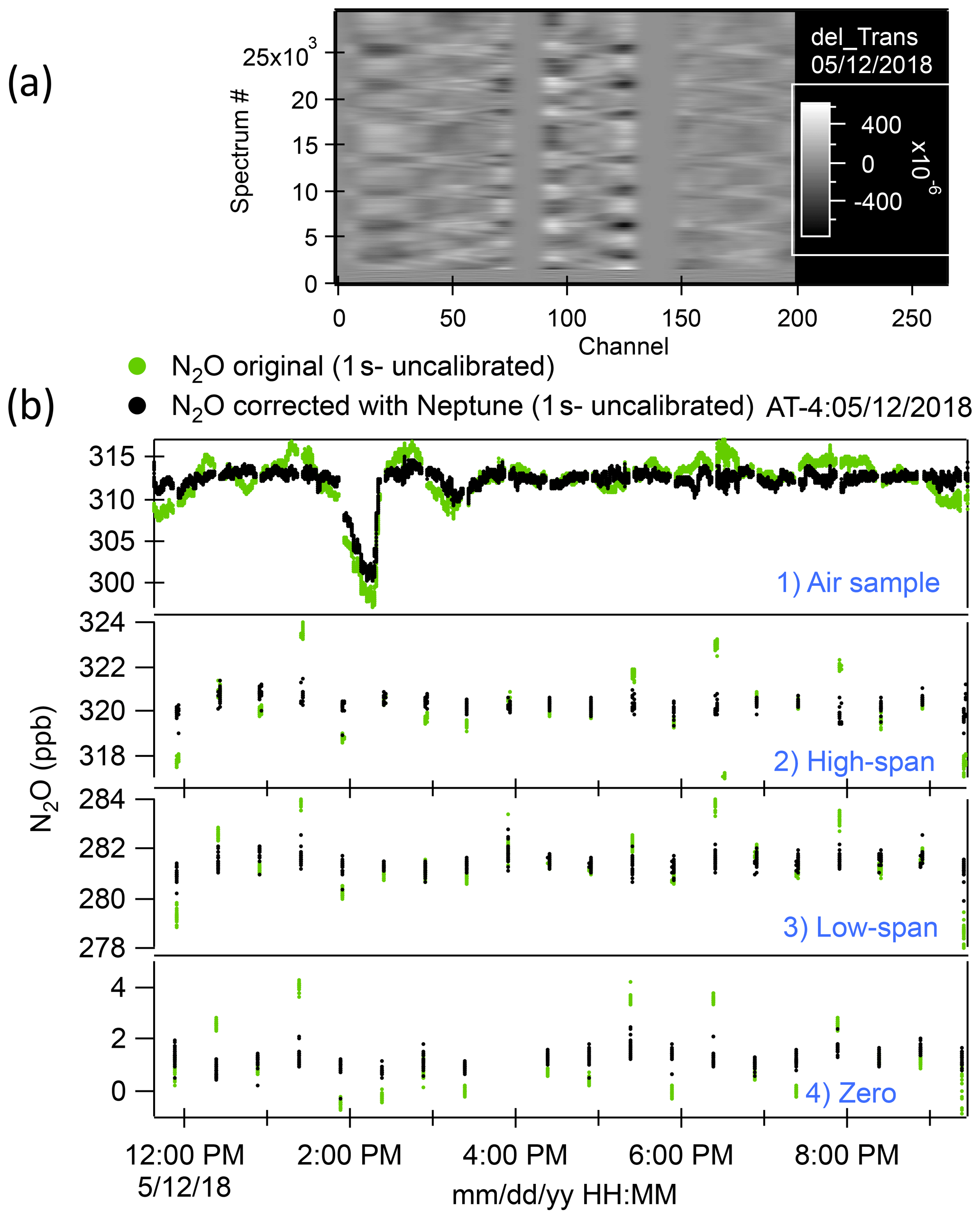
Figure 1 (a) A processed spectral array from the ATom-4 flight on 12 May 2018. “Channel” represents a point number in the spectra. Spectra have been grouped by type (i.e., calibration or ambient), with averages subtracted, absorption lines zeroed out (near channels 75, 140, and 225). This residual spectral array is then smoothed with a binomial filter where the filter width corresponds to the linewidth of the original spectra. Shifts in fringe phases during altitude changes are apparent. (b) Time series of ambient air samples and high-span, low-span, and zero calibrations for the same flight as (a). Green dots are the original N₂O data record. Black dots are the N₂O data corrected with Neptune (no calibration applied at this point).

Figure 2 (a) Comparisons between Neptune-corrected QCLS N₂O and (1) UCATS N₂O, (2) PANTHER N₂O, and (3) PFP N₂O for ATom-2 (orange circles), ATom-3 (green stars), and ATom-4 (blue squares). We used the 10 s averaged merged file to compare QCLS, UCATS, and PANTHER data. The PFP flask samples had longer sampling times (30 s to a few minutes). The 1:1 line is shown as a dashed line. (b) Comparisons between NOAA N₂O surface flask measurements and Neptune-corrected and airborne data from (1) QCLS N₂O, (2) UCATS N₂O, (3) PANTHER N₂O, (4) and PFP N₂O for ATom-2, -3, and -4, similar to (a1)–(a3). The solid line shows the 1:1 relationship + offset. For plots (b1)–(b4), the airborne data are the mean N₂O values within ± 5^∘ of latitude of each surface station and between 1 and 4 km.

3 Accuracy of N₂O measurements from QCLS

We evaluated N₂O mixing ratios measured by QCLS against three other instruments that measured N₂O on the NASA DC-8 aircraft during ATom. In addition, we compared the set of four airborne measurements to data from the flask sampling network at ground stations from the NOAA Global Monitoring Laboratory (GML, https://gml.noaa.gov/, last access: 10 December 2020) to evaluate the differences between the airborne data and the ground-based measurements in the NOAA reference network.

3.1 Comparison between airborne N₂O measurements

Measurements of N₂O on the DC-8 during ATom were obtained by four instruments: (i) the Unmanned Aircraft Systems Chromatograph for Atmospheric Trace Species (UCATS, Hintsa et al., 2021), (ii) the PAN and other Trace Hydrohalocarbon ExpeRiment (PANTHER; Moore et al., 2006; Wofsy et al., 2011), (iii) the Programmable Flask Package Whole Air Sampler (PFP; Montzka et al., 2019), and (iv) our 1 Hz QCLS.

We compared QCLS, PANTHER, and UCATS at 10 s intervals, as provided in the ATom merged file MER10_DC8_ATom-1.nc available at the Oak Ridge National Laboratory Distributed Active Archive Center (ORNL-DAAC, Wofsy et al., 2018, https://doi.org/10.3334/ORNLDAAC/1581, last access: 28 February 2021). The ATom file MER-PFP merged with the PFP sampling interval (also available in the above repository) was used to compare QCLS and PFP data. A one-to-one comparison between these instruments showed an approximately 1 ppb positive bias in N₂O mixing ratios from QCLS (see Fig. 2a1–a3). The 95 % confidence interval of the mean difference for each pair (95 % C.I.) was 0.75 ± 0.04 ppb between QCLS and PANTHER, 1.13 ± 0.03 ppb between QCLS and UCATS, and 1.18 ± 0.09 ppb between QCLS and PFP, respectively, for the full data set (ATom-2, -3, and -4). Information about the coefficients of the linear fit for each instrument comparison and the 95 % C.I. of the difference for each pair are shown in Table S2. The offset that QCLS N₂O shows against PFP N₂O coincides with the offset already reported by Santoni et al. (2014) during HIPPO in 2009–2011, which may be attributed to our calibration procedure. PFP flasks are considered the reference measurement on board as the flasks are analyzed with excellent precision and accuracy.

3.2 Comparison between airborne and surface measurements of N₂O

We evaluated the traceability of lower-troposphere N₂O mixing ratios by ATom by comparing the four airborne instruments with the surface measurements of N₂O from the NOAA flask sampling network. If a surface station was encountered within a latitude range of 5^∘ north and south with respect to the flight track during a flight, that surface station was used in the study.

The mean value of N₂O within that latitude grid of ± 5^∘ and at instrument altitudes of 1–4 km was compared with the mean N₂O observed at the surface station during the period ± 5 d relative to the flight (due to the non-daily frequency of flask samples). We chose the altitude range between 1 to 4 km to agree with the low free tropospheric conditions that characterized most of the selected ground stations. Information about the surface stations used here is shown in Table S3 of the Supplement.

The comparison of the whole data set (ATom-2, -3, -4) shows that, overall, QCLS and PANTHER overestimated N₂O mixing ratios with respect to the surface data by 1.37 ± 0.35 and 0.44 ± 0.51 ppb (95 % C.I.), respectively. In contrast, UCATS and PFP showed low bias with respect to the surface data: 0.27 ± 0.37 and 0.008 ± 0.34 ppb (95 % C.I.), respectively (Fig. 2b1–b4). Due to the excellent agreement between PFP and the surface stations and the consistent offset that QCLS showed against PFP and the stations, the QCLS N₂O data presented in the following sections of this publication were corrected by subtracting the offset with respect to the PFP data onboard in each deployment: 1.03 ± 0.13 ppb in AT-2, 1.49 ± 0.19 ppb in AT-3, and 1.18 ± 0.17 ppb in AT-4. The final official archive data file includes a new column where these corrections have been applied (N₂O_QCLS_ad).

These results show the very close comparability of the ATom airborne N₂O instruments (differences were < 0.5 ppb for UCATS and PANTHER instruments and 0 ppb in the case of PFP) relative to the surface stations and demonstrate the feasibility of using ATom N₂O measurements to evaluate the impact of stratospheric air and meridional transport of N₂O emissions on N₂O tropospheric column measurements over the ocean basins. In the following section, we define the boundary conditions that were used to evaluate that impact, which were based on the NOAA Greenhouse Gas Marine Boundary Layer Reference from the NOAA GML Carbon Cycle Group (NOAA/ESRL GML CCGG, https://gml.noaa.gov/, last access: 10 December 2020). The NOAA-MBL N₂O product is a synthetic latitude profile generated at 0.05 sine latitude and weekly resolution from individual flask measurements of marine boundary-layer surface stations distributed along the two ocean basins, and provides the scenario needed to evaluate the traceability of aircraft measurements relative to ground measurements at remote sites (https://gml.noaa.gov/ccgg/arc/?id=13, last access: 10 December 2020).

4 Results and discussion

The vertical profiles of N₂O from ATom provide a global overview of the N₂O distribution in the troposphere, with observations performed over the Pacific and Atlantic basins. For this study, we do not include data collected over and close to land. In ATom, N₂O ranged between 280 and 335 ppb over the oceans. In each season, the lowest N₂O mixing ratios are observed at high latitudes (HL, > 60^∘) in the UT/LS (8–12.5 km), in air transported downward from the stratosphere. The highest N₂O mixing ratios are found close to the Equator (30^∘ S–30^∘ N, 326 to 335 ppb), and extend along the tropospheric column up to 6 km. They are influenced by convective activity over the tropical regions (Kort et al., 2011; Santoni et al., 2014). At mid-latitudes (ML, 30–60^∘ N), tropospheric N₂O values range between 322 and 333 ppb. Tropospheric N₂O tends to increase towards northern latitudes as a result of higher anthropogenic emissions in the Northern Hemisphere relative to the Southern Hemisphere. More details on the variability of N₂O mixing ratios along the tropospheric column are described in Sect. S1.

We study the impact of N₂O sources and stratospheric air on the N₂O column based on the anomalies (enhancements and depletions) we observed in the airborne N₂O mixing ratios relative to the N₂O “background,” defined here as the NOAA-MBL product. We use the NOAA-MBL product to constrain a latitudinal gradient of N₂O mixing ratios at the surface for each deployment. These data have been widely used to estimate the N₂O background (Assonov et al., 2013; Nevison et al., 2011). More information about the NOAA-MBL product and the latitudinal gradient of their measurements is discussed in Sect. S2. This approach highlights the extra information that aircraft profiles can provide. Cross-sections of N₂O anomalies are shown in Fig. 3. The data describe the overall homogeneity of N₂O in the troposphere (30 % of the anomalies ranged between ± 0.5 ppb). We suppose that the ± 0.5 ppb interval accounts for the day-to-day and seasonal variability of N₂O. Episodes of N₂O depletion (< −0.5 ppb) that relate to the influence of stratospheric air are observed in 53.5 % of the aircraft samples during ATom-2 to -4, whereas episodes of N₂O enhancement (> 0.5 ppb) that relate to the contribution of N₂O sources account for 16.5 % of the calculated anomalies.

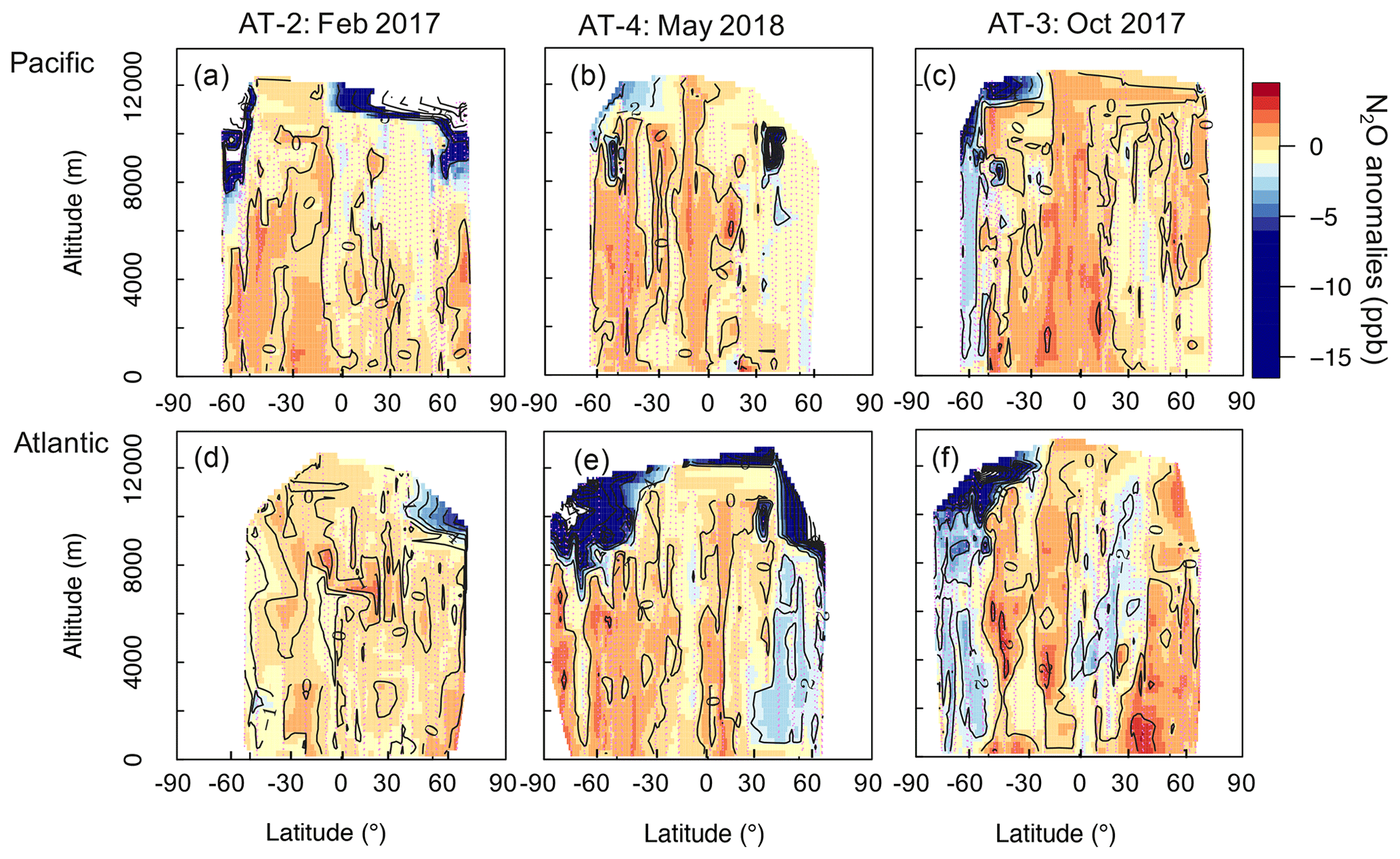
Figure 3 Cross-sections of N₂O anomalies (ppb) representing the differences between the airborne N₂O (10 s resolution) and the surface N₂O mixing ratios, interpolated to 0.25^∘ latitude and 250 m altitude for each deployment. Shown are the N₂O anomalies over (a)–(c) the Pacific and (d)–(f) the Atlantic, with each column representing a deployment (ordered by season: ATom-2, -4, and -3). The color scale ranges from −15 to 5 ppb. Values between −50 and −15 ppb, observed at the highest altitudes (> 10 km), are shown in white to allow better visualization of small changes in positive anomalies. Lilac dashed lines represent the flight tracks. Black contours are areas of N₂O anomalies.

Trajectories and associated surface influence functions were computed using the Traj3D model (Bowman, 1993) and wind fields from the National Center for Environmental Prediction Global Forecast System (NCEP GFS). Model trajectories were initialized at receptors spaced 1 min apart along the ATom flight tracks, followed backwards for 30 d, and reported at 3 h resolution. From these trajectories, we calculated the surface influence for each receptor point (footprints in units of concentration mixing ratio per emission flux; ppt nmol⁻¹ m² s). The footprint can be convolved with a known flux inventory of a nonreactive gas to calculate the expected enhancement/depletion of that gas for each receptor point.

4.1 Impact of stratospheric air on tropospheric N₂O mixing ratios during ATom

We observe the strongest depletions (> 5 ppb) in N₂O mixing ratios at high latitudes and altitudes, consistent with stratospherically influenced air (Fig. 3). Stratosphere–troposphere exchange processes allow stratospheric-depleted N₂O to be distributed throughout the troposphere. The NOAA surface network shows a seasonal minimum of N₂O 2–4 months later than the stratospheric polar vortex break-up season. This seasonal minimum is observed at the surface around May in the Southern Hemisphere and around July in the Northern Hemisphere (see Figs. S8 and S9) (see Nevison et al., 2011 and references therein). The enhanced downwelling of the Brewer–Dobson circulation (BDC) in late winter–spring reinforces the downward transport of stratospheric air depleted in N₂O throughout the free troposphere (1–8 km), as observed in October in the Southern Hemisphere (ATom-3, Fig. 3c and f) and in May in the North Atlantic (ATom-4, Fig. 3e). The N₂O depletion is likely the result of stratospheric air being moved downwards by the BDC and trapped by the polar vortex, with a more pronounced effect in the Southern Hemisphere, where the polar vortex is stronger. These results support previous work suggesting that downward transport of stratospheric air with low N₂O exerts a strong influence on the variance of tropospheric N₂O mixing ratios (Nevison et al., 2011; Assonov et al., 2013).

The impact of stratosphere-to-troposphere transport can be studied by combining information on tracers of stratospheric air such as ozone (O₃ from the NOAA – NO_yO₃; Bourgeois et al., 2020), sulfur hexafluoride (SF₆ from PANTHER), CFC₁₂ (from PANTHER), and carbon monoxide (CO from QCLS). These tracers are usually used either because they are strongly produced in the stratosphere (e.g., O₃) or because they are tracers of anthropogenic emissions in the troposphere with a strong stratospheric sink (e.g., CO, SF₆, and CFC₁₂). In addition, meteorological parameters such as potential vorticity (PV), the product of absolute vorticity and thermodynamic stability (PV was generated by GEOS5-FP for ATom), can be used to trace the stratosphere-to-troposphere transport.

Overall, the interhemispheric gradient of N₂O is much smaller than those of CO and SF₆ (Fig. 4), but the difference for each species is driven by larger anthropogenic emissions in the Northern Hemisphere. The tracer–tracer correlations shown in Fig. 4 show different patterns. The linear trend between N₂O and O₃ or CFC-12 highlights the role of depletion (N₂O and CFC-12) and production (O₃) in the stratosphere (Fig. 4a1, a4). When N₂O is plotted against the anthropogenic tracers CO and SF₆, two distinct trends are observed. Tropospheric N₂O can be identified as the horizontal band containing high N₂O (> 328 ppb) and variable CO and SF₆, whereas the vertical band with variable N₂O and small changes in CO and SF₆ is due to the mixing between tropospheric air and stratospheric air depleted in N₂O (Fig. 4a1–a3). The N₂O versus CO plot shows an L-shaped (bimodal) curve similar to those typically observed in O₃–CO correlations during stratosphere-to-troposphere airmass mixing events (Fig. 4a2, Krause et al., 2018). A quasi-vertical line in the N₂O–CO plot (i.e., constant CO) is indicative of a strong impact of stratospheric air, as the stratospheric equilibrium mixing ratio of CO is observed (Krause et al., 2018). The lower the CO background, the greater the influence of the stratospheric air during the airmass mixing (North Atlantic high latitudes in Fig. 4a2) and vice versa. A strong correlation is also indicative of rapid mixing between the two air masses. During ATom, the strongest impact of stratospheric air was observed in the Pacific mid- and high latitudes in February (ATom-2) and in the Atlantic in May (ATom-4, Fig. S11). At the North Pacific mid- and high latitudes (NMHL > 30^∘ N), we find a consistent linear relationship between N₂O and O₃, with a relatively constant N₂O $/$ O₃ slope (−0.05 to −0.04) during all seasons. Linear correlations between N₂O and CFC-12 highlight the dominant influence of stratospheric air that was depleted in these two substances in the range of mixing ratios observed at mid- and high latitudes (Fig. S11).

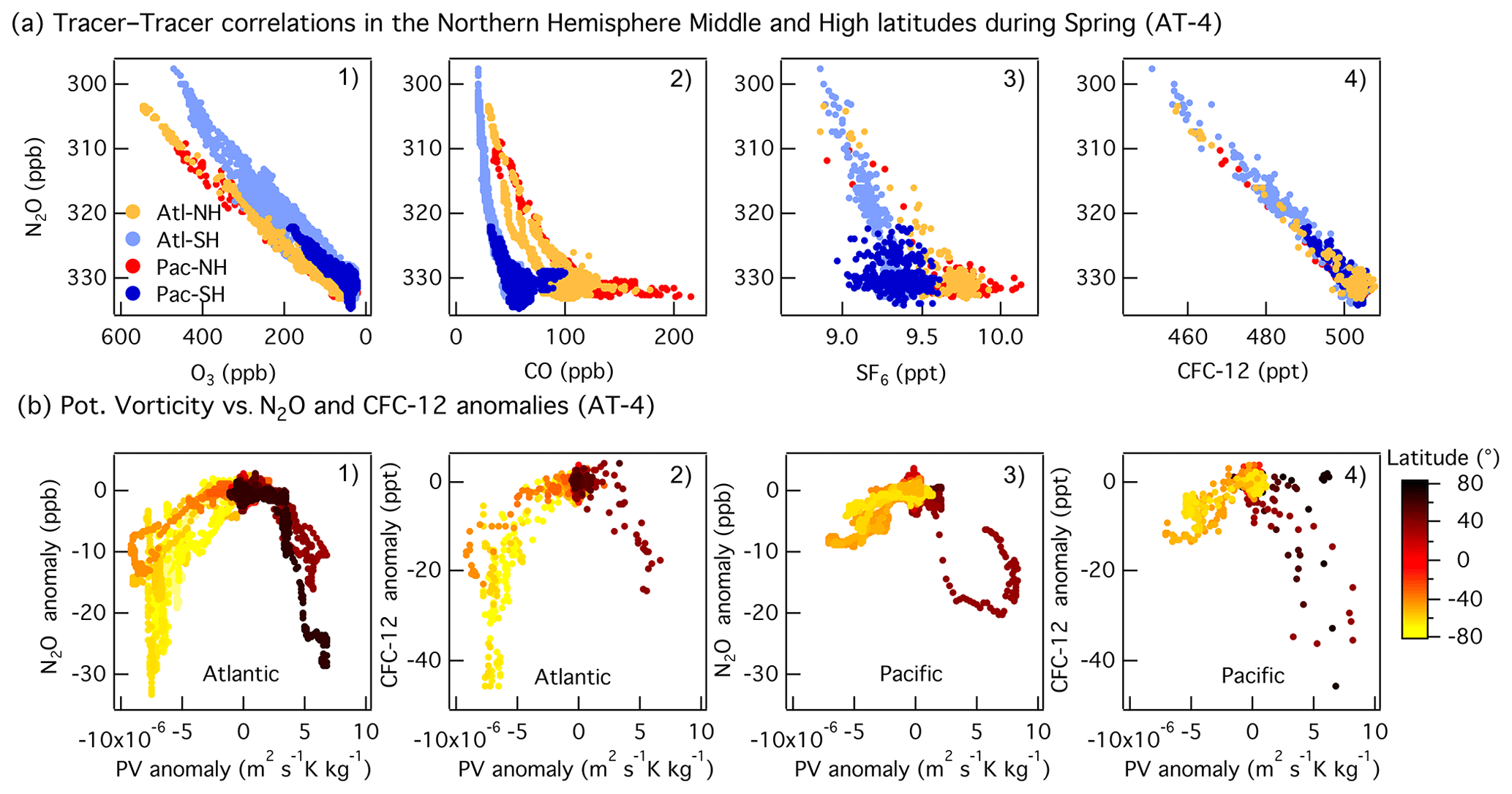
Figure 4 (a) Correlations between N₂O and O₃ (a1), CO (a2), SF₆ (a3), and CFC-12 (a4) at mid- and high latitudes (30–85^∘ N) during Northern Hemisphere spring (ATom-4). The data are colored as a function of the ocean basin and hemisphere: North Pacific mid–high latitudes (Pac-NH, > 30^∘ N) in red, South Pacific mid–high latitudes (Pac-SH, < 30^∘ S) in dark blue, South Atlantic mid–high latitudes (Atl-SH, < 30^∘ S) in light blue, and North Atlantic mid–high latitudes (Atl-NH, > 30^∘ N) in orange. Note that the N₂O and O₃ axes are reversed. (b) Correlations between anomalies in potential vorticity relative to its mean latitudinal distribution in the free troposphere (2–8 km) and anomalies in N₂O (b1, b3) and CFC-12 (b2, b4) as a function of latitude during spring (ATom-4) over the Pacific and Atlantic basins. Mid-latitudes are shown in orange in the SH and in light brown in the NH.

During spring, the mid-latitudes are strongly impacted by stratospheric air due to the occurrence of tropopause folds and cutoff lows to the south of the westerly subtropical jets (Hu et al., 2010 and references therein). The stronger depletion of N₂O mixing ratios observed over the Atlantic relative to the Pacific during spring is due to a greater number of deep stratosphere-to-troposphere transport events at mid-latitudes in the region between May and July (Fig. 3e; Cuevas et al., 2013 and references therein). Anomalies in PV relative to its mean latitudinal distribution in the free troposphere (2–8 km) highlight events involving the strong downward transport of stratospheric air. Negative PV, N₂O, CO, and CFC-12 anomalies (positive for O₃) describe the transport of stratospheric air into the troposphere in the SH, whereas positive PV and negative N₂O, CO, and SF₆ anomalies (positive for O₃) describe the downward transport of stratospheric air in the NH (Fig. 4b1–b4). The correlations between N₂O and PV and the similarities with CFC-12 indicate that stratosphere-to-troposphere exchange leads to variations in tropospheric N₂O of up to 10 ppb at the higher latitudes for the altitudes covered during the flights. This influence is notably larger than the 2–4 ppb enhancements associated with regional emissions (see below).

4.2 Impact of emissions on tropospheric N₂O mixing ratios during ATom

During ATom, episodes of positive N₂O anomalies relative to the surface station MBL reference occurred close to the equator (Fig. 3a–c) and in a few locations at mid-latitudes in both ocean basins across all seasons. We used the information from the vertical profiles, including back trajectories and correlated chemical tracers, to trace the origins of these enhancements. We investigated data on CO, CH₄, and CO₂ measured by QCLS and NOAA Picarro 2401 m; hydrogen cyanide (HCN), sulfur dioxide (SO₂), hydrogen peroxide (H₂O₂), and peroxyacetic acid (PAA) measured with the California Institute of Technology Chemical Ionization Mass Spectrometer (CIT-CIMS, Crounse et al., 2006; St. Clair et al., 2010); ammonium (NH${}_{\mathrm{4}}^{+}$), sulfate (SO${}_{\mathrm{4}}^{\mathrm{2}-}$), nitrate (NO${}_{\mathrm{3}}^{-}$), and organic aerosols (OA) from the Colorado University Aircraft High-Resolution Time-of-Flight Aerosol Mass Spectrometer (HR-AMS, DeCarlo et al., 2006; Canagaratna et al., 2007; Jimenez et al., 2019; Guo et al., 2021; Hodzic et al., 2020); NO_y from the NOAA NO_yO₃ four-channel chemiluminescence instrument (CL, Ryerson et al., 2019); CH₂Br₂, CH₃CN, benzene, and propane from the NCAR Trace Organic Gas Analyzer (TOGA, Apel et al., 2019); and atmospheric potential oxygen (APO ≈ O₂+1.1 × CO₂) from the NCAR Airborne Oxygen Instrument (AO2, Stephens et al., 2020).

We calculated the correlations between N₂O and the mentioned species in three layers (0–2000, 2000–4000, and 4000–6000 m). Correlation coefficients in each layer for a given profile were calculated using a minimum threshold of 15 data points per layer. These profiles show that many of the most prominent enhancements of N₂O are closely associated with pollutants such as HCN, CH₃CN, H₂O_2,, and other pollutants associated with combustion and photochemical air pollution. Some profiles show peaks that are closely correlated with SO₂ and enhanced PM1 particles, and vertical gradients were sometimes correlated with gradients of APO and HCN.

Several N₂O peaks are observed together with enhancements of H₂O₂ and PAA, which are primarily formed in chemical processes that occur in the atmosphere. For the altitude range 2–4 km, regressions produced r² > 0.7 for 16 profiles of N₂O vs. H₂O₂ and 15 profiles of N₂O vs. HCN (a tracer for combustion of biomass), but only three such profiles produced these strong associations for both H₂O₂ and HCN in common. Some of these profiles also showed correlated enhancements of SO₂ and NO (nine profiles with r² > 0.6). This result raises the question of whether globally significant production of N₂O may be occurring in heterogeneous reactions involving SO₂, NO redox chemistry, and HONO near to strong sources of reactive pollutants, which have been observed in heavily polluted atmospheres (Wang et al., 2020) and have been theorized to occur in the plumes of refineries or power plants (e.g., Pires and Rossi, 1997).

In most cases, because we were sampling in the middle of each ocean and not over the source regions, it was not possible to distinguish between the different sources that contributed to the observed N₂O enhancements. We also observed that the impacts of the different sources on N₂O mixing ratios were region dependent. Here, we describe, with some examples, the sources that contribute to the major N₂O enhancements observed during ATom by oceanic region, although we cannot precisely pinpoint the source processes.

4.2.1 N₂O enhancements over the Pacific

Episodes of N₂O enhancement were frequently observed at mid-latitudes in the southern Pacific Ocean, and these were linked by the associated footprints to emissions over the continents. In this region, N₂O enhancements are predominantly associated with air masses with enhanced H₂O₂, PAA, and CO. For example, consider Fig. 5, which shows data from profile 12, obtained at 49.5–50^∘ S and near the Date Line on 3 May 2018. A distinct peak in N₂O of amplitude 1 ppb at 1700 m altitude is significantly correlated with enhancements in CH₃CN. These associations and the footprints suggest a regional contribution from fuel types from the industrial zone of Australia (Fig. 5c), which is also supported by the aerosol characterization from PALMS (not shown for brevity). In this profile, close to the surface, the lowest QCLS N₂O mixing ratios agree with the NOAA MBL N₂O (dashed line in Fig. 5b). At higher altitudes (2.5–6 km), strong correlations between N₂O, H₂O₂, PAA, CO, and HCN but not SO₂ suggest the influence of biomass burning from central Australia (3–5 km) and South America (6 km) (Fig. 5b, middle and right-hand panels in Fig. 5c, and Fig. S11f). The relatively low mixing ratios of short-lived trace gases (PAA, H₂O₂, and PM1 aerosols with lifetimes ranging from hours to a few days) and the surface influence based on the back trajectories (Fig. S13a) indicate that most of these profiles sampled significantly aged air masses that were transported for extended periods over the South Pacific.

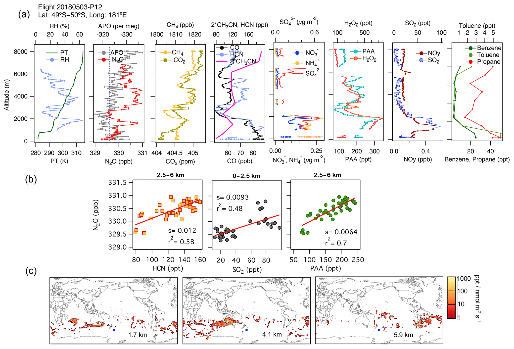
Figure 5 (a) Vertical profiles of potential temperature (PT), relative humidity (RH), N₂O, APO, CH₄, CO₂, CO, HCN, CH₃CN, NO${}_{\mathrm{3}}^{-}$, NH${}_{\mathrm{4}}^{+}$, SO${}_{\mathrm{4}}^{\mathrm{2}+}$, H₂O₂, PAA (CH₃C(O)OOH), SO₂, NO_y, benzene, toluene, and propane from profile 12, obtained on 3 May 2018. The dotted blue line in the plot of APO and N₂O represents the NOAA-MBL reference (N₂O-MBL) at the latitude of the flight. (b) Correlations between N₂O and HCN and PAA for altitudes between 2.5 and 6 km, and between N₂O and SO₂ for altitudes between 0 and 2.5 km, indicate an admixture of marine, biomass-burning, urban, and oil and gas industry contributions to N₂O mixing ratios (s represents the slope of the linear fit). (c) Footprint maps tracing surface regions that influence mixing ratios measured at the altitude ranges of 1–2, 2.5–5, and 5–7 km, respectively. Blue squares show sampling locations. Values below 3 ppt nmol⁻¹ m² s are not included. Note that the APO axes are reversed.

In the equatorial Pacific, episodes of N₂O enhancement were frequently associated with a mixture of potential marine, industrial, and biomass burning emissions. Atmospheric potential oxygen (APO) is primarily a tracer of oxygen exchange with the oceans, defined as deviations in the oxygen-to-nitrogen ratio (δ(O₂ $/$ N₂)) corrected for changes in O₂ due to terrestrial photosynthesis and respiration and for influences from combustion (Stephens et al., 1998),

$$\begin{array}{}\text{(1)}& \mathit{\delta }\mathrm{APO}=\mathit{\delta }\left({\mathrm{O}}_{\mathrm{2}}/{\mathrm{N}}_{\mathrm{2}}\right)+\mathrm{1.1}/X_{{\mathrm{O}}_{\mathrm{2}}}(X_{{\mathrm{CO}}_{\mathrm{2}}}-\mathrm{350}).\end{array}$$

Here, δ(O₂ $/$ N₂) is the deviation in the O₂ $/$ N₂ ratio (per meg), 1.1 is an approximation to the O₂ $/$ CO₂ ratio for photosynthesis and respiration, $X_{{\mathrm{O}}_{\mathrm{2}}}$ is the mole fraction of O₂ in dry air, and $X_{{\mathrm{CO}}_{\mathrm{2}}}$ is the mole fraction of CO₂ in the air sample (dry, µmol mol⁻¹). Since APO primarily tracks oxygen exchange between the ocean and the atmosphere, APO depletions can indicate marine N₂O emissions from areas with strong upwelling (Lueker et al., 2003; Ganesan et al., 2020). However, APO is also sensitive to pollution such as biomass burning and fossil fuel combustion (Lueker et al., 2001) and, because both N₂O and APO have meridional gradients resulting from many influences, correlations can result simply from sampling air transported from different latitudes. In ATom, nine profiles showed significant correlations (r² > 0.7) between N₂O and APO (or δ(O₂ $/$ N₂), which has lower measurement noise) for altitude bins 0–2 (8) and 2–4 km (1), with back trajectories indicating that they originated close to the west coast of North America and the Mauritanian coast as well as in the equatorial Pacific. The median slope of regressions of APO vs. N₂O for these profiles in ATom is −0.04 ppb per meg, and the mean is −0.05 (± 0.04, 1σ) ppb per meg – very similar to the range found by Ganesan et al. (2020) and Lueker et al. (2003) in coastal areas.

An example is shown in Fig. 6 for 1 May 2018. We observe a high correlation between N₂O and APO (r²=0.66) between 0 and 4 km altitude. At these altitudes we also see enhancements in dibromomethane (CH₂Br₂), a tracer of phytoplankton biomass (Liu et al., 2013 and references therein), consistent with a marine biological flux of halogenated VOCs (Asher et al., 2019), dimethyl sulfide (DMS), and methanesulfonic acid (MSA), the main particulate product of DMS oxidation in the MBL. However, on this flight, the footprints and the influence of the surface ocean (Fig. S12b) indicate that this N₂O gradient represents a difference between sampling a near-surface marine air mass from the south and a more continental air mass from the east at 4 km (Fig. 6a–c). Close to the surface, the lowest QCLS N₂O mixing ratios agree with the NOAA MBL N₂O at the origin of the air masses suggested by the footprints (25^∘ S, dashed red line in Fig. 6b), whereas the lowest QCLS N₂O mixing ratios at 4 km agree with the NOAA MBL N₂O (dotted blue line in Fig. 6b). Thus, the N₂O to APO correlation most likely represents the latitudinal and ocean–land gradients established for a combination of reasons, with higher APO and lower N₂O originating from higher southern latitudes away from continents. During this flight, there were particularly noticeable N₂O variations between 4 and 6 km height that appear to be related to biomass-burning plumes from fires occurring in Venezuela and the Caribbean, in agreement with simultaneous enhancements in CO and HCN mixing ratios (Fig. 6a, c and Fig. S12), and there was increasing SO₂ in the first 2 km, which was linked to oil and gas pollution sources near coastlines. The nature of these emissions was also confirmed by aerosol characterization using the PALMS instrument (figure not shown).

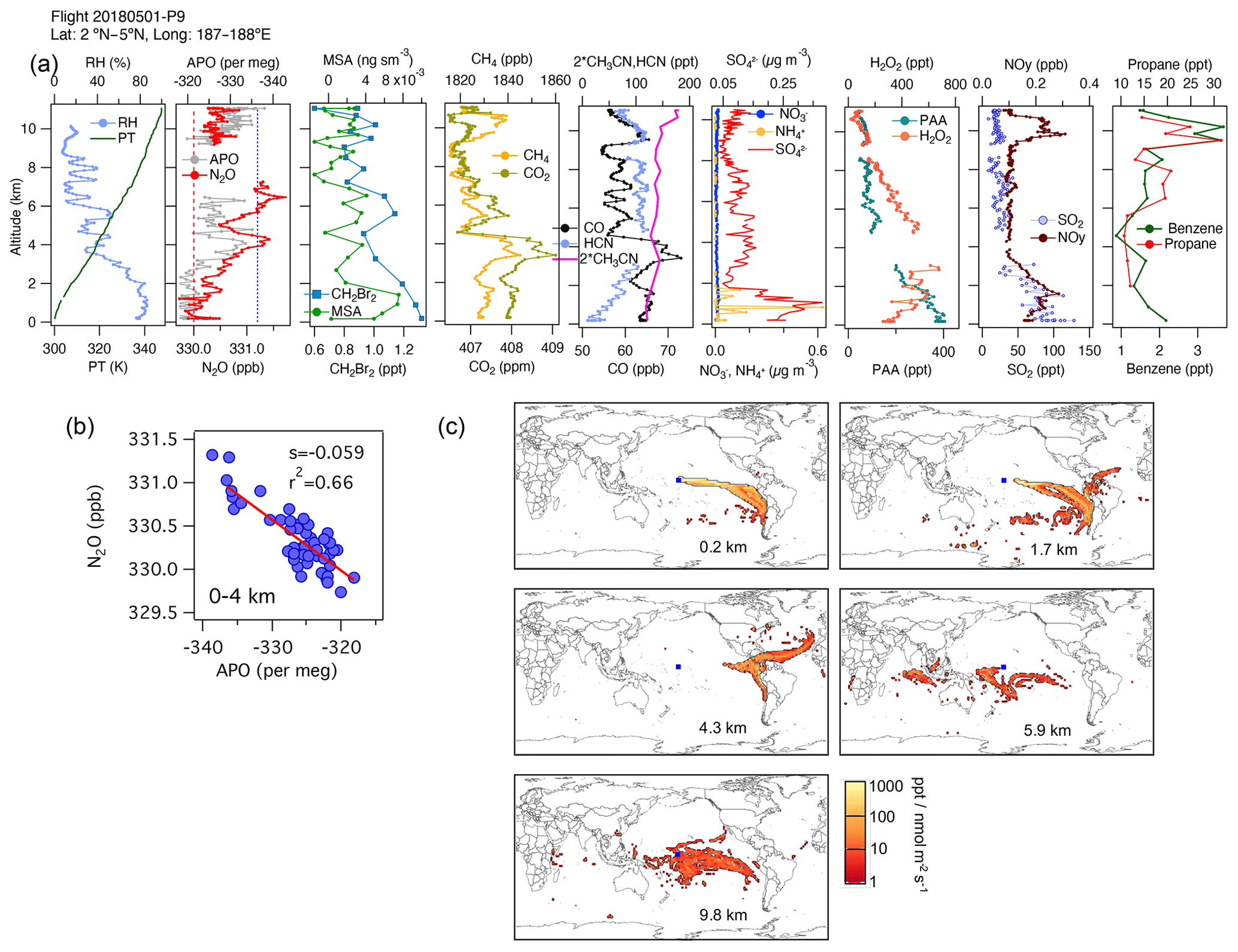
Figure 6 (a) Vertical profiles of PT, RH, and the tracers N₂O, APO, MSA, CH₂Br₂, CH₄, CO₂, CO, HCN, CH₃CN, NO${}_{\mathrm{3}}^{-}$, NH${}_{\mathrm{4}}^{+}$, SO${}_{\mathrm{4}}^{\mathrm{2}-}$, H₂O₂, PAA (CH₃C(O)OOH), SO₂, NO_y, benzene, toluene, and propane from profile 9 on 1 May 2018. The dotted blue line in the plot of APO and N₂O represents the NOAA-MBL reference (N₂O-MBL) at the latitude of the flight; the dashed red line shows the N₂O-MBL at the origin of the air masses suggested by the footprints (25^∘ S). (b) N₂O–APO correlations between 0 and 4 km that possibly describe the latitudinal gradient of N₂O (s represents the slope of the linear fit). (c) Footprint maps tracing surface regions that influence mixing ratios measured in the altitude ranges 0–2, 2–4, 3–5, 5–7, and 9–11 km, respectively. Blue squares show sampling locations. Values below 3 ppt nmol⁻¹ m² s are not included. Note that the APO axes are reversed to illustrate the negative correlation with N₂O.

4.2.2 N₂O enhancements over the Atlantic

Much more of a continental influence was observed during the Atlantic Basin ATom flights than during the Pacific flights. In the North Atlantic at around 30^∘ N during winter, we observe small enhancements of N₂O that contrast with the overall influence of stratospheric air on the tropospheric column (AT-2, Fig. 3d). The contribution is much higher during the fall season (AT-3, Fig. 3f). Several episodes of N₂O enhancement are associated with enhancements of CH₄, CO, and HCN. We also observe some episodes where N₂O increases while CO₂ decreases (figure not shown), which could reflect the accumulation of agricultural emissions over the summer or just greater sampling of Northern Hemisphere summer air masses, whereas increases of N₂O with CO are indicators of urban pollution and are, together with HCN, associated with a few episodes of biomass burning.

The influences of different regions on the N₂O mixing ratios over the Atlantic on 14 May 2018 are shown in Fig. 7. This profile shows the contributions to tropospheric N₂O from pollution transported down over the Mauritanian coast from Western Europe, biomass-burning emissions, urban and industrial emissions from southern Africa and the Middle East (between 1.5 and 3 km), and polluted air masses from South America and the west coast of Africa, which are mixed with the oceanic contribution to N₂O (∼ 10 km, Fig. 7a–c and Fig. S13). The aerosol characterization (from PALMS, not shown) indicates that mineral dust and biomass-burning emissions influence the atmospheric layer between 1 and 6 km in altitude, while oil combustion influences the layer below 4 km. At high altitudes, N₂O enhancements are caused by the interception of polluted air masses from South America and the west coast of Africa mixed with the oceanic contribution to N₂O (∼ 10 km). The N₂O:APO correlations for the feature between 1.5 and 3 km most likely represent APO depletion through industrial combustion, which is stoichiometrically consistent with the observed increases in CO₂ and CH₄ for this feature.

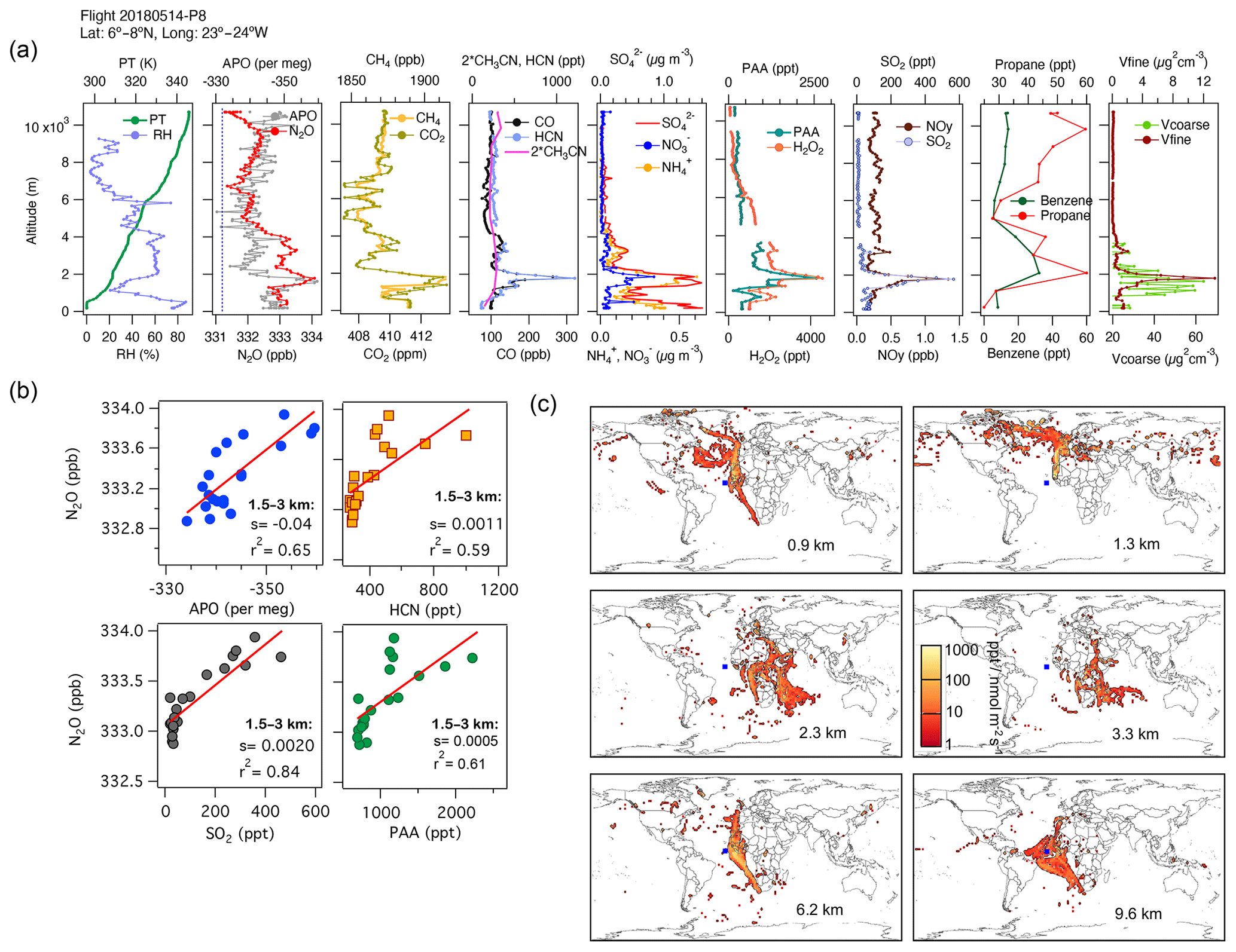
Figure 7 (a) Vertical profiles of PT, RH, the tracers N₂O, APO, CH₄, CO₂, CO, HCN, CH₃CN, NO${}_{\mathrm{3}}^{-}$, NH${}_{\mathrm{4}}^{+}$, SO${}_{\mathrm{4}}^{\mathrm{2}-}$, H₂O₂, PAA, SO₂, NO_y, benzene, and propane, and the volumes of coarse and fine particles from profile 8 on 14 May 2018. The dotted blue line in the plot of APO and N₂O represents the NOAA-MBL reference (N₂O-MBL) at the latitude of the flight. (b) Correlations between N₂O and APO, HCN, SO₂, and propane at altitudes of 1–3 km show possible contributions from marine upwelling, biomass burning, and the oil and gas industry, as supported by the footprints (s represents the slope of the linear fit). (c) Footprint maps tracing surface regions that influence mixing ratios measured in the altitude ranges 0–1, 2–4, 4–5, 5–7, and 7–10 km, respectively. The blue square shows the sampling location. Values below 3 ppt nmol⁻¹ m² s are not included. Note that the APO axes are reversed.

During ATom, we observed large contributions to the tropospheric N₂O over the Atlantic Ocean from Africa, along with some contributions from Europe and South America. During AT-2, we found strong correlations in the subtropical and tropical regions over the Atlantic between N₂O, H₂O₂, PAA, HCN, CO, CO₂, SO₂, OA, NH${}_{\mathrm{4}}^{+}$, and SO${}_{\mathrm{4}}^{\mathrm{2}-}$ at altitudes between 0 and 2.5 km, representing the combined influence of photochemistry ($r_{\mathrm{N}\mathrm{2}\mathrm{OvsPAA}}^{\mathrm{2}}=\mathrm{0.94}$), biomass-burning events from the Congo region ($r_{\mathrm{N}\mathrm{2}\mathrm{OvsHCN}}^{\mathrm{2}}=\mathrm{0.95}$), and the industrial production of N₂O from oil and gas emissions from the Niger River Delta in Africa ($r_{\mathrm{N}\mathrm{2}\mathrm{OvsSO}\mathrm{2}}^{\mathrm{2}}=\mathrm{0.84}$). An example is shown in Fig. 8 for 15 February 2017 (see also Fig. S12 and the land contribution in Fig. S13).

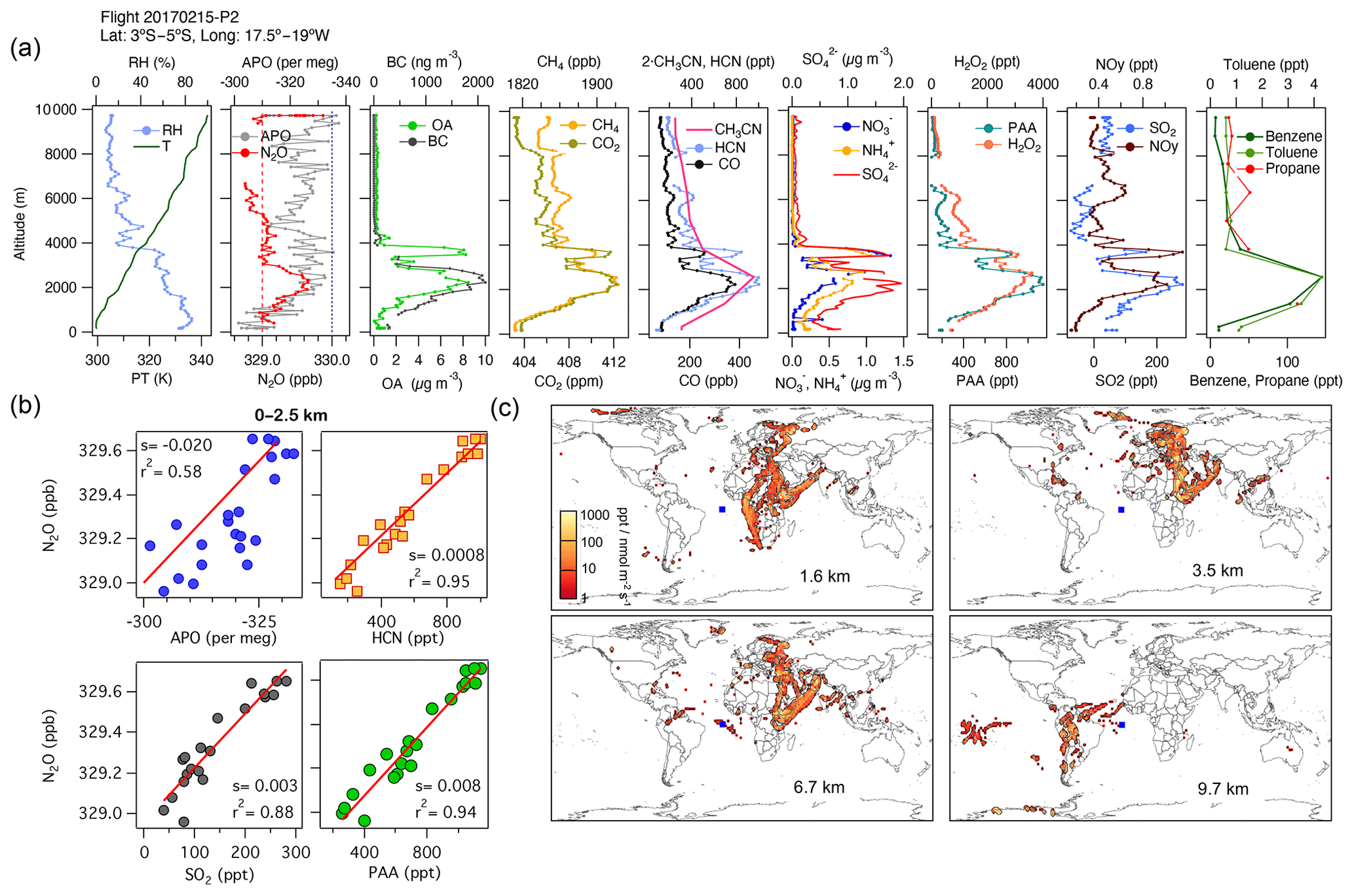
Figure 8 (a) Vertical profiles of PT, RH, and the tracers N₂O, APO, organic aerosols (OA), black carbon (BC), CH₄, CO₂, CO, HCN, CH₃CN, NO${}_{\mathrm{3}}^{-}$, NH${}_{\mathrm{4}}^{+}$, SO${}_{\mathrm{4}}^{\mathrm{2}+}$, H₂O₂, PAA, SO₂, NO_y, benzene, toluene, and propane from profile 2 on 15 February 2017. The dotted blue line in the plot of APO and N₂O represents the NOAA-MBL reference (N₂O-MBL) at the latitude of the flight, and the red dashed line shows the NOAA-MBL at the origin of the southern air masses shown by the footprints below 2 km (20^∘ S). (b) Correlations between N₂O and APO, HCN, and SO₂ for data observed below 2.5 km indicate an admixture of marine, biomass-burning, urban, and oil and gas industry contributions to N₂O mixing ratios (s represents the slope of the linear fit). (c) Footprint maps tracing surface regions that influence mixing ratios measured in the altitude ranges 0–2, 2–3, 3–4, and 4–7 km, respectively. Blue squares show sampling locations. Values below 3 ppt nmol⁻¹ m² s are not included in the footprint plot. Note that the APO axes are reversed.

To understand the origin of the enhancements in N₂O, we calculated the enhancement expected in the atmosphere based on monthly mean estimates of anthropogenic emissions from the Emissions Database for Global Atmospheric Research (EDGAR, http://edgar.jrc.ec.europa.eu/, last access: 5 February 2021). We convolved the calculated surface influence (footprint) with the inventory to calculate the N₂O enhancement expected for each receptor. We also calculated the contribution of each region and source sector to the overall enhancement. This allowed us to quantify the dominant sources for various layers within each profile. Each of the calculated enhancements was then compared to the enhancement in N₂O observed for the profiles. The observed N₂O enhancements were calculated relative to the NOAA MBL reference (Fig. 8a, dashed red line) for each 10 s observation, with background concentrations selected from locations close to the origin of the air mass as indicated by the surface influence (shown as dashed and dotted lines in the N₂O altitude profiles in Figs. 5–8). We also included 0.4 ppb of uncertainty for the observed enhancements based on our measurement precision.

Figure 9 N₂O enhancements estimated by EDGAR for the entire globe (gray polygons) and for the African region (blue polygons), and the observed QCLS-N₂O enhancement relative to the NOAA-MBL N₂O reference at the origin of the southern air masses shown by the footprints below 2 km for the profile 2017/02/15-P2 (20^∘ S, 329 ppb, shown in Fig. 8). QCLS-N₂O was observed every 10 s and receptors were calculated every 60 s.

The largest N₂O enhancement (peaking at 2 ppb at 2 km) observed over the Atlantic during ATom-2 (February 2017; Fig. 9) can be attributed to African agriculture, along with smaller but significant influences from Asia and Europe (0.5 ppb each at 2–4 km, Fig. S14). The observed and modeled N₂O enhancements agree within an order of magnitude for the profile, but the model underestimates the high-altitude (4–7 km) N₂O enhancement by < 1 ppb and overestimates the lower-altitude enhancement (2–4 km) by ∼ 1 ppb. This difference in N₂O enhancement could be due to a strong latitudinal gradient in N₂O across this profile or the timing of N₂O emissions sampled along this single profile compared to a monthly mean estimate from the inventory. Strong correlations between N₂O and HCN (r²=0.95), CO, and CH₃CN suggest that N₂O from burning emissions also contributes to the N₂O enhancement (Figs. 8 and S12). However, when we convolved the monthly mean fire contributions from the Global Fire Emissions Database (GFED, https://www.globalfiredata.org, last access: 5 February 2021) with the surface influence footprints (as described above), we found that the wildfire-produced N₂O is minimal for this profile (∼ 0.2 ppb), suggesting that fires of anthropogenic or urban origin might be the source of that contribution (Figs. 8a–c, 9, S12, and S13).

5 Conclusions

N₂O mixing ratios at 1 Hz were obtained during the NASA ATom airborne program by applying a new spectral retrieval method to account for the pressure and temperature sensitivity of quantum cascade laser spectrometers deployed on aircraft. This method improved the precision of our QCLS N₂O measurements by a factor of three (based on the standard deviation of calibration measurements), allowing us to provide N₂O measurements to the level of precision shown in previous aircraft missions.

The N₂O altitude profiles observed during ATom show that tropospheric N₂O variability is strongly driven by the influence of stratospheric air depleted in N₂O, especially at mid- and high latitudes. At high latitudes, our profiles showed a strongly depleted N₂O signal around the time of the vortex break-up season, persisting for several months. Combining the information from N₂O profiles and other chemical tracers such as CO, SF₆, O₃, and CFC-12, we traced the propagation of stratospheric air along the tropospheric column down to the surface. This transport dominates the N₂O seasonal cycle and creates the seasonal surface minima 2–3 months after the peak stratosphere–troposphere exchange in spring.

The high resolution of this data set (10 s) allowed us to study the factors influencing the enhancements in the N₂O tropospheric mixing ratios, which are associated with biomass burning and human activities such as urban and industrial emissions. The highest N₂O mixing ratios occur close to the Equator, where they extend throughout the tropospheric column. The strongest N₂O enhancements were observed close to the Equator and at a number of mid-latitude locations. We used the information given by the vertical profiles of N₂O and a variety of chemical tracers together with footprints computed every 60 s along the flight track to identify and trace the sources of these N₂O enhancements. N₂O enhancement events were more frequent in the Atlantic than in the Pacific.

Over the Atlantic, the co-occurrence of excess N₂O together with other pollutants suggested that industrial and urban N₂O emissions originating from distant locations such as western and southern Africa, the Middle East, Europe, and South America may be significantly greater than the emissions from biomass burning in Africa. This view is supported by our observations of a strong contribution to N₂O from oil and gas emissions from the Niger River Delta in Africa. The correlations observed between N₂O and SO₂ (r²=0.90) could possibly be used to estimate N₂O emissions from oil and gas.

Over the southern Pacific Ocean and the tropical Atlantic Ocean, we observed a significant number (> 12) of profiles where enhancements in N₂O were associated with increased H₂O₂ and PAA and notably less well correlated with HCN or CO. Since H₂O₂ and PAA are products of photochemical pollution, this observation raised the question of whether significant N₂O may be produced by heterogeneous processes involving HONO or NO_x reactions in acidic aerosols close to sources or in very heavily polluted areas. It is hard to draw a definite conclusion based on measurements obtained so far from the most active regions. Studies performed to address this question would have to be carried out directly in the polluted areas. Because agricultural activities do not have unique tracer signatures, we were not able to distinguish contributions from cultivated and natural soils to N₂O emissions from the ATom data. Previous airborne studies have observed these inputs using flights in agricultural areas (Kort et al., 2008) and at towers in these regions (e.g., Nevison et al., 2017; Miller et al., 2008).

Our study shows that airborne campaigns such as ATom can help trace the origins of biomass-burning and industrial emissions and investigate their impact on the variability of tropospheric N₂O, providing unique signatures in vertical profiles and with covariate tracers. We hope that the information provided by the global tropospheric N₂O profiles from the ATom mission will help better diagnose and reduce uncertainties in atmospheric chemical transport models for constraining the N₂O global budget.

Appendix A: List of frequently used symbols and acronyms

Description	Acronym
Atmospheric Potential Oxygen	APO
Atmospheric Tomography	ATom
California Institute of Technology – Chemical Ionization Mass Spectrometer	CIT-CIMS
CU Aircraft High-Resolution Time-of-Flight Aerosol Mass Spectrometer	HR-AMS
Global Monitoring Laboratory	GML
HIAPER Pole-to-Pole Observations	HIPPO
High Latitudes	HL
HIgh-resolution TRANsmission molecular absorption database	HITRAN
Marine Boundary Layer	MBL
Middle Latitudes	ML
Modern-Era Retrospective analysis for Research and Applications 2 model	MERRA2
National Center for Environmental Prediction Global Forecast System model	NCEP GFS
National Oceanic and Atmospheric Administration	NOAA
NCAR Airborne Oxygen Instrument	AO2
NOAA Halocarbons and other Atmospheric Trace Species Flask Sampling Program	NOAA-HATS
NOAA NOyO3 4-channel chemiluminescence	CL
Northern Hemisphere	NH
PAN and other Trace Hydrohalo-carbon ExpeRiment	PANTHER
Particle Analysis by Laser Mass Spectrometry instrument	PALMS
Potential Vorticity	PV
Principal Component Analysis	PCA
Programmable Flask Package Whole Air Sampler	PFP
Quantum Cascade Laser Spectrometer	QCLS
Southern Hemisphere	SH
Stochastic Time-Inverted Lagrangian Transport Model	STILT
Trace Organic Gas Analyzer	TOGA
Unmanned Aircraft Systems Chromatograph for Atmospheric Trace Species	UCATS
Upper Troposphere/Lower Stratosphere	UT/LS
World Meteorological Organization	WMO