Spectrometric measurements of atmospheric propane (C₃H₈)

We report measurements of atmospheric C₃H₈ from analysis of ground-based solar absorption spectra from the Jet Propulsion Laboratory (JPL) MkIV interferometer. Using the strong Q-branch absorption feature at 2967 cm⁻¹, we can measure C₃H₈ in locations where its abundance is enhanced by proximity to sources (e.g., large natural gas fields, megacities). A case study of MkIV C₃H₈ measurements from Fort Sumner, New Mexico, shows that amounts are strongly correlated with ethane (C₂H₆) and with back-trajectories from SE New Mexico and western Texas, where the Permian Basin oil and natural gas field is located. Measurements from JPL, California, also show large C₃H₈ enhancements on certain days but more correlated with CO than C₂H₆. From high-altitude balloon-borne MkIV solar occultation measurements, C₃H₈ was not detected at any altitude (5–40 km) in any of the 25 flights.

1 Introduction

Non-methane hydrocarbons such as C₃H₈ and C₂H₆ affect air quality, because their oxidation enhances tropospheric O₃ and aerosol pollution. They are also sensitive indicators of fugitive losses by the oil and natural gas industry and an important source of co-emitted methane (CH₄), which is a greenhouse gas. These fugitive losses appear to be underestimated in global inventories (Dalsøren et al., 2018).

Atmospheric C₃H₈ and C₂H₆ are entirely the result of emissions at the surface. In preindustrial times these came from geological seeps and wild fires, but in recent times these natural sources have been surpassed by emissions from fossil fuel production. The latter peaked in about 1970 and then declined due to stricter regulation of emissions from the oil and natural gas industry and automobiles. But in the past decade, this decreasing trend has reversed due to accelerated natural gas (NG) exploitation (Helmig et al., 2016).

C₃H₈ has a lifetime of about 2 weeks in summer and 8 weeks in winter (Rosado-Reyes and Francisco, 2007). This is mostly dictated by how fast it is being oxidized by reactions with hydroxyl radicals and chlorine atoms. Given this 2–8-week lifetime, a single strong source of propane has the potential to degrade air quality over most of the hemisphere.

Unprocessed in-the-ground “wet” natural gas is usually between 70 %–95 % CH₄, 1 %–15 % C₂H₆, 1 %–10 % C₃H₈, and 0 %–3 % C₄H₁₀. The last two gases are typically extracted to form liquified petroleum gas (LPG). In the Northern Hemisphere (NH) winter, LPG contains more C₃H₈, while in summer it contains more butane (C₄H₁₀), reducing variations in its vapor pressure.

LPG burns much more cleanly than fuel oil and is therefore increasingly used for heating and cooking, especially in rural areas that are not served by piped NG. LPG is also used to fuel commercial vehicles, and it is increasingly replacing CFCs as a refrigerant and as an aerosol propellant. As a result of extracting LPG from natural gas, the NG that is piped to our homes in urban areas is highly depleted in C₃H₈ and C₄H₁₀, as compared with wet NG.

To the best of our knowledge, there are no previous remote sensing measurements of C₃H₈, although in situ measurements exist. Dalsøren et al. (2018, Fig. 3b) show surface in situ C₃H₈ amounts below 50 ppt at Zeppelin station in Svalbard in summer 2011 but with values of 1 ppb in the winter and with peaks of up to 2.4 ppb. These C₃H₈ peaks are strongly correlated with C₂H₆ which reaches 3.4 ppb. Using in situ C₃H₈ data from multiple sites Helmig et al. (2016) show a large seasonal cycle in surface in situ C₃H₈ at high NH latitudes, reaching 1 ppb in winter with little in the Southern Hemisphere (SH). They also show increasing C₃H₈ over central and eastern US over the period mid-2009 to mid-2014 but no increase on the west coast.

Since C₃H₈ correlates with C₂H₆, both having NG as their main source, we also consider the previous measurements of C₂H₆, which has a lifetime of 2–8 months (4 times longer than propane). Angelbratt et al. (2011) reported a 0 %–2 % yr⁻¹ decline over the period 1996 to 2006 based on data from six NH FTIR sites. Franco et al (2015) reported a shallow minimum in C₂H₆ in the 2005–2010 period based on ground-based FTIR solar spectra above the Jungfraujoch scientific station. Helmig et al. (2016) report a minimum in atmospheric C₂H₆ in 2005–2010 based on in situ and remote measurements.

Franco et al. (2016) estimate a 75 % increase in North American C₂H₆ emissions between 2008 and 2014, and as a result they report a 3 %–5 % annual increase in column C₂H₆ at northern mid latitudes. They hypothesize that this increase is the result of the recent massive growth in the exploitation of shale gas and tight oil reservoirs in North America, where the drilling productivity began to grow rapidly after 2009.

2 Methods

2.1 MkIV instrument

The Jet Propulsion Laboratory (JPL) MkIV interferometer (Toon, 1991) is a high-resolution FTIR spectrometer built at JPL in 1984. It covers the entire 650–5650 cm⁻¹ range simultaneously in every spectrum with two detectors: a HgCdTe photoconductor covering 650–1800 cm⁻¹ and an InSb photodiode covering 1800–5650 cm⁻¹. For ground-based observations, a maximum optical path difference (OPD) of 117 cm is employed, providing a spectral resolution of 0.005 cm⁻¹. The MkIV is primarily a balloon instrument and has performed 25 flights since 1989, with the latest in 2019. Between balloon flights it makes ground-based observations. Since 1985 it has taken 5000 ground-based observations on 1200 different days from 12 different sites. For more detail, see tables in the following URL: https://mark4sun.jpl.nasa.gov/ground.html, last access: 20 June 2021.

2.2 Retrieval

The analysis of the MkIV spectra was performed with the GFIT (gas fitting) tool, which is a nonlinear least-squares spectral-fitting algorithm developed at JPL. GFIT has been previously used for the version 3 analysis (Irion et al., 2002) of spectra measured by the Atmospheric Trace Molecule Occultation Spectrometer, and it is currently used for analysis of Total Carbon Column Observing Network (TCCON) spectra (Wunch et al., 2011) as well as for MkIV spectra (Toon et al., 2016, 2018a, b). The entire package, including spectral fitting software, spectroscopic line lists, and software to generate a priori VMR $/$ T $/$ P profiles, is termed GGG.

GFIT scales the atmospheric gas volume mixing ratio (VMR) profiles to fit calculated spectra to those measured. For C₃H₈, a 5.4 cm⁻¹ wide fitting window centered on the Q-branch at 2967 cm⁻¹ was used. The atmosphere was discretized into 70 layers of 1 km thickness. C₃H₈ and four interfering gases (H₂O, CH₄, C₂H₆, HDO) were adjusted. Two frequency stretches were retrieved (telluric and solar). The spectral continuum was fitted as a straight line, and a zero-level offset was fitted. So that is a total of 10 simultaneously fitted scalars. In addition, the solar pseudo-transmittance was computed (but not adjusted).

The assumed temperature, pressure, and H₂O profiles were based on the National Centers for Environmental Prediction (NCEP) 6-hourly analyses for solar noon of each day. The a priori VMR profiles were based on NH mid-latitude profiles. This is the same scheme as used by the GGG TCCON analysis (Wunch et al., 2015), but here we apply it to the mid-IR MkIV spectra rather than the shortwave IR TCCON spectra.

To estimate the sensitivity of the retrieved C₃H₈ to uncertainties in the assumed a priori profiles of $T/P$ and interfering gases (especially H₂O, CH₄), we retrieve the post-2000 C₃H₈ a second time: using GGG2020, an updated version of the GGG code with improved a priori VMR $/$ T $/$ P profiles based on the GEOS-FP-IT analysis. The results, shown in Fig. B2, illustrate that this changes the retrieved C₃H₈ by less than 10 % with a bias of only 1.1 %.

2.3 Spectroscopy

It is clear from the infrared lab spectrum of C₃H₈ (Fig. 1), measured at Pacific Northwest National Laboratory (PNNL; Sharpe et al., 2004), that the feature at 2967 cm⁻¹, caused by various CH₂ and CH₃ stretching vibrational modes, is by far the strongest in the entire infrared. So for solar occultation spectrometry, this is by far the best choice. For thermal emission spectrometry from cold astronomical bodies such as Titan, however, these bands are not covered by Cassini/CIRS since the thermal Plank function of such bodies weakens rapidly above 2000 cm⁻¹. Thus, the much weaker bands below 1400 cm⁻¹ must be used (Sung et al., 2013).

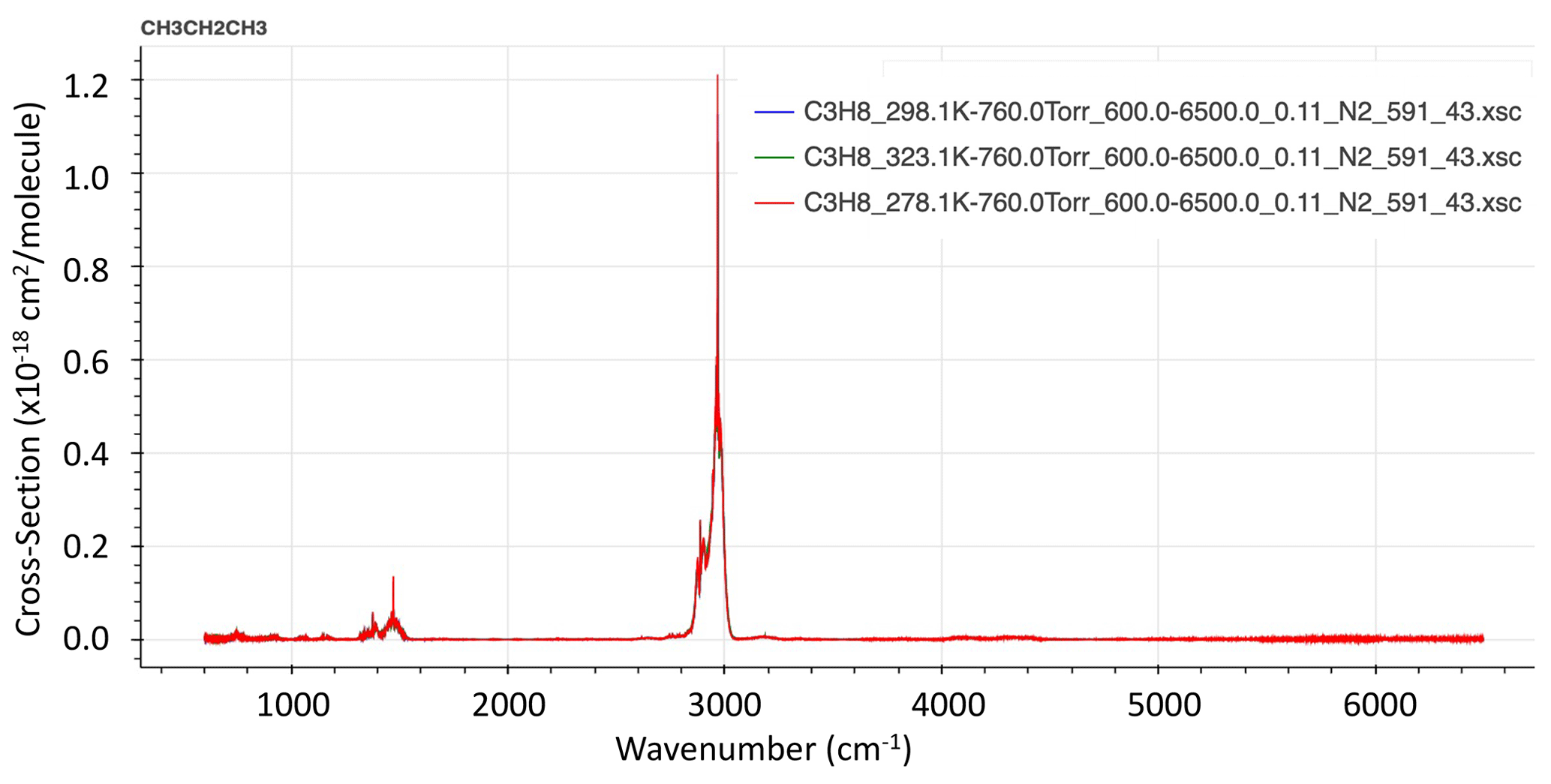
Figure 1 Infrared spectra of PNNL C₃H₈ absorption cross section at 323, 298, and 278 K (from hitran.org).

An empirical pseudo-line-list (EPLL) of C₃H₈ covering 2560–3280 cm⁻¹ was derived from the laboratory cross sections of Harrison and Bernath (2010). This is described in the following unpublished report: https://mark4sun.jpl.nasa.gov/data/spec/Pseudo/c3h8_pll_2560_3280.pdf, last access: 20 June 2021.

The use of an EPLL facilitates interpolation and extrapolation of the lab cross sections to $T/P$ conditions that were not measured in the lab. The fitting of the EPLL also checks the self-consistency of the lab cross-section spectra and provides an opportunity for us to correct for artifacts in the lab spectra (e.g., channeling, zero-level offsets, contamination, instrument line shape (ILS), although it must be stated that in this particular case the C₃H₈ lab spectra were of very high quality and comprehensive in terms of their coverage. For the interfering C₂H₆, an EPLL developed 8 years ago was used, based on lab measurements of Harrison et al. (2010), as described in the following report: https://mark4sun.jpl.nasa.gov/report/C2H6_spectroscopy_evaluation_2850-3050_cm-1.compressed.pdf, last access: 20 June 2021.

For other gases, the atm.161 line list was used, which is based on HITRAN 2016, with some empirical adjustments based on fits to lab spectra, especially for H₂O and CH₄. This is basically the same line lists (atm.161, pll.101) that are used by TCCON, but here we use them in the mid-infrared (MIR) rather than the shortwave infrared (SWIR).

Figure 2 shows an average spectral fit to the C₃H₈ window in ground-based MkIV spectra, obtained by fitting individual spectra and then averaging the results. The lower panel provides the full transmittance y range from 0 to 1. It can be seen that the main absorbers are CH₄ (orange) and H₂O (green). The C₃H₈ absorption (red) is difficult to discern, because it is so shallow. The lower-middle panel shows the same spectral fit but with the y scale zoomed into 0.95–1.00 transmittance, allowing the weak absorbers like C₃H₈ and C₂H₆ to be more easily seen. The “other” contributions (e.g., O₃) were included in the calculation but not adjusted. The C₃H₈ absorption is fairly flat at about 1 % depth, except for the Q-branch where it deepens to 2.5 %. Although the strongest C₂H₆ feature coincides with the C₃H₈ Q-branch, the former is much narrower and there are several additional C₂H₆ features in this window, so the spectrometric “cross-talk” between these two gases should be modest; we compute a Pearson correlation coefficient of −0.7 between the C₃H₈ and C₂H₆. Further discussion on this topic can be found in Appendix A. The upper-middle panel shows that the residuals (measured minus calculated transmittance) have some systematic features of ∼ 0.5 % in magnitude, especially in the vicinity of the H₂O line at 2966.0 cm⁻¹. The topmost panel shows the residuals to a fit performed without any C₃H₈ absorption lines. It looks surprisingly similar to the fit performed with C₃H₈ lines, such is the ingenuity of the spectral fitting algorithm in adjusting the H₂O, CH₄, and C₂H₆ to compensate for the missing C₃H₈. The overall rms residual in the no-C₃H₈ case is 0.3934 %, as compared with 0.3658 % when C₃H₈ is included. This is quite significant considering that residuals are dominated by the H₂O line at 2966.0 cm⁻¹ and are unaffected by whether C₃H₈ is included or not. The residuals in the topmost panel (d) are larger in the vicinity of the C₃H₈ Q-branch, 2967–2968 cm⁻¹, than those in panel (c).

Considering the weakness (and smoothness) of the C₃H₈ Q-branch in comparison with the residuals and the contributions of the other gases, we were at first skeptical that a useful C₃H₈ column measurement could be extracted from such spectral fits. But since the analysis of the MkIV spectra is highly automated, it took only a few hours to run the C₃H₈ window over all 5000 MkIV ground-based spectra.

3 Results

Table 1 lists the observation sites from where MkIV has made ground-based observations up to the end of 2019. The vast majority are from three sites: JPL, Mount Barcroft, and Fort Sumner.

Table 1 The 12 sites from where MkIV has made ground-based observations, along with the number of observations and observation days from each site, years of operations, their location, and terrain type. The unbold sites have the fewest observations (only 1 % of total) and are not included in Figs. 5–7 and A1 to reduced color ambiguity.

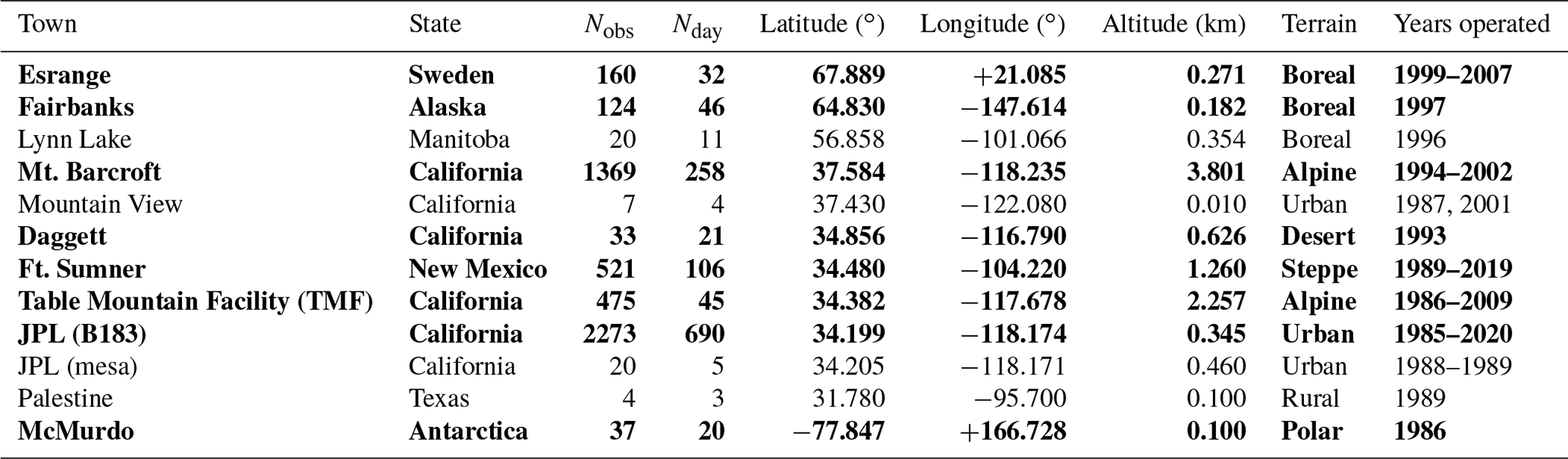
Figure 3 shows MkIV ground-based C₃H₈ columns, color-coded by site altitude. The data were filtered: only points with uncertainties <1.5×10¹⁶ molecules cm⁻² were plotted, reducing the number of plotted points from 5000 to 4700. The top panel (a) shows that at the high-altitude sites (Mt. Barcroft at 3.8 km is red; Table Mountain Facility at 2.26 km is orange) the retrieved C₃H₈ columns are centered around zero. Also, the data acquired in September 1986 from 0.1 km in Antarctica (dark blue) are centered around zero. Data acquired from Ft. Sumner, New Mexico, at 1.2 km (lime green) have large variations, from zero to nearly 8×10¹⁶ molecules cm⁻², as do the data from JPL at 0.35 km (cyan). Other sites with detectable C₃H₈ include Daggett, California (0.6 km); Esrange, Sweden (0.26 km) in the winter; Fairbanks, Alaska (0.2 km); and Mountain View, California, in late 1991. So C₃H₈ has only been measured by MkIV from Northern Hemisphere sites within the planetary boundary layer (PBL). Panels (b) and (c) show the same C₃H₈ columns but plotted versus year and day.

High C₃H₈ values (>4×10¹⁶ molecules cm⁻²) can occur at any time of year at JPL (cyan) but most commonly in late summer, as is the case for other pollutants, e.g., CO. This reflects the meteorology (stagnant conditions in the LA basin in summer with little replacement of polluted air with clean air from outside). Averaging kernels for these C₃H₈ measurements are discussed and illustrated in Appendix B. Suffice it to say here that they range from 0.9 to 1.4 and increase with altitude.

The reported uncertainties in our C₃H₈ column measurements are based on the rms fitting residuals compared with the sensitivity of the spectrum to C₃H₈ (Jacobians). At the highest site, Mt. Barcroft at 3.8 km (P=0.65 atm), where the interfering H₂O and CH₄ absorptions are relatively weak and narrow, the C₃H₈ column uncertainties are generally smaller than 10¹⁵ molecules cm⁻². But since the columns themselves are even smaller, no C₃H₈ is detected at Mt. Barcroft. At the lower-altitude sites such as JPL and Ft. Sumner, the increased interference from H₂O and CH₄ cause the C₃H₈ column uncertainties to be much larger, generally around 5×10¹⁵ molecules cm⁻² at low air mass and worsening rapidly toward higher air masses. But the C₃H₈ increases far more, allowing C₃H₈ to be detected at these low-altitude sites under polluted conditions, despite the poorer absolute uncertainties.

High C₃H₈ values are also seen at Ft. Sumner, New Mexico (lime green), especially in recent years. This was initially a surprise to us as this area has a very low population density, so we naively assumed that we would be measuring background levels of atmospheric pollutants here.

We know that the apparent variations in C₃H₈ are real, rather than artifacts, from their strong correlation with C₂H₆. Figure 4 compares column-averaged C₃H₈ mole fractions (top panels) with those of C₂H₆ (bottom panels), with the latter retrieved using different spectral lines than those shown in Fig. 2. These are the same total C₃H₈ columns shown in Fig. 3 but divided by the total column of all gases, which is inferred from the surface pressure. The resulting column-average mole fractions, denoted Xgas, are less sensitive to the site altitudes being different and more easily compared with in situ measurements being in units of mole fraction.

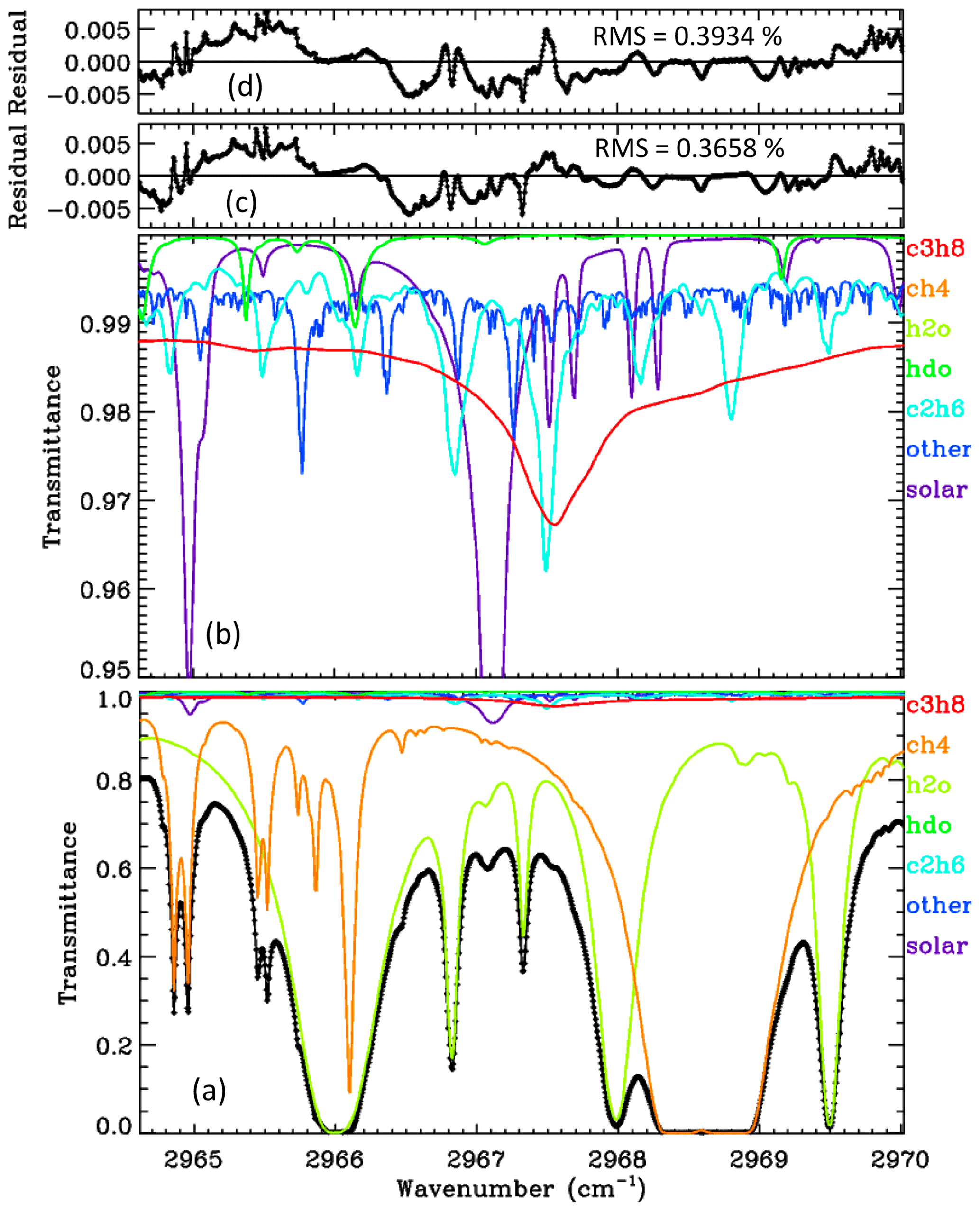
Figure 2 The average of 5000 ground-based MkIV spectral fits. Black diamonds represent the measured spectrum. Black line represents the fitted calculation. Colored lines represent the contributions of different gases. Panel (a) shows the full transmittance range. Panel (b) shows a zoomed-in view of the 0.95–1.00 range to clearly show the weak absorbers (C₂H₆, HDO, and the solar lines). Panel (c) shows residuals (measured minus calculated); these are generally below 0.5 %. Panel (d) shows the residuals when C₃H₈ is excluded from the calculation.

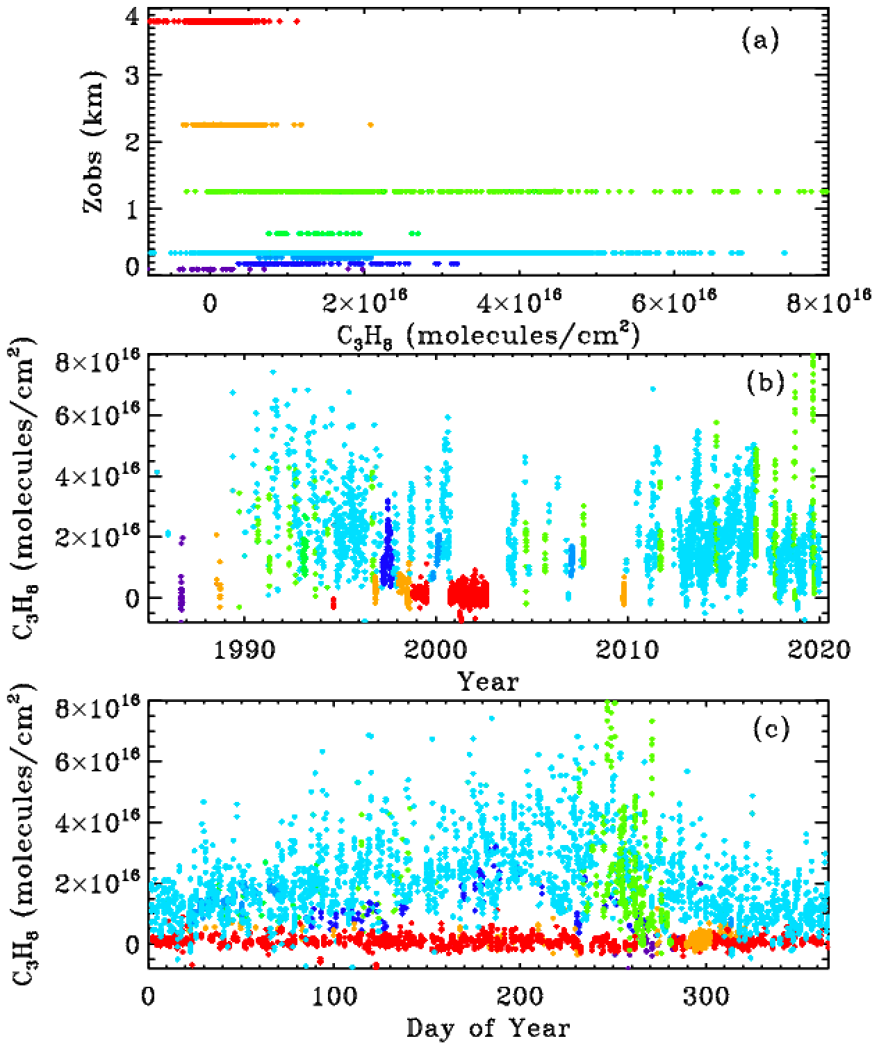
Figure 3 MkIV C₃H₈ column abundances from 8 out of 12 sites, color-coded by site altitude, as illustrated in panel (a): violet = 0.1 km (McMurdo); dark blue = 0.18 km (Fairbanks); light blue = 0.27 km (Esrange); cyan = 0.35 km (JPL); green = 0.63 km (Daggett); lime green = 1.2 km (Ft. Sumner); orange = 2.26 km (TMF); red = 3.8 km (Mt. Barcroft).

The upper and lower rows of Fig. 4 show the XC₃H₈ and XC₂H₆ time series, respectively, plotted versus year (left) and versus day of the year (right). The data were filtered such that only points with XC₃H₈ uncertainties <0.74 ppb and C₂H₆ uncertainties <0.10 ppb were plotted. This reduced the total number of points from 5000 to 4700, so only the best 94 % of the data are plotted. It is clear that at JPL (cyan) C₃H₈ has decreased since the 1990s, but at Ft. Sumner (lime green) it has increased over the past decade. The data from these two sites will be explored later.

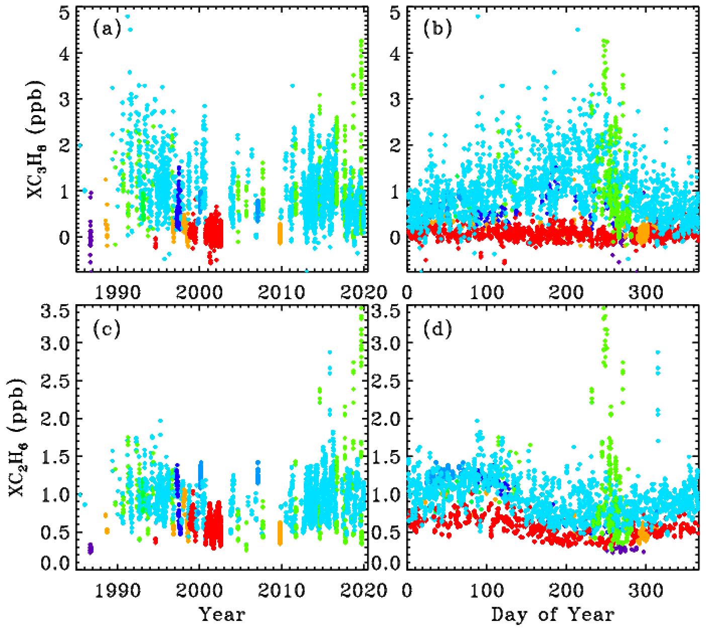
Figure 4 Top panels (a, b) show measurements of the column-averaged C₃H₈ mole fractions (XC₃H₈). Bottom panels (c, d) show XC₂H₆. Left-hand panels (a, c) show the variation with year. Right-hand panels (b, d) show the seasonal variation. Points are color-coded by observation site altitude, as in Fig. 3.

C₂H₆ is 4 times longer-lived than C₃H₈ and never goes to zero, because there is always a substantial free tropospheric C₂H₆ component, even in the SH, which varies seasonally: high in spring and low in fall. The Antarctic measurements (blue) are very low (0.2–0.3 ppb) and most probably even lower during the rest of the year, because days 250 to 300 represent the springtime peak not the fall. The highest C₂H₆ ever measured from JPL (cyan) was in late 2015 (day 314) as a result of the Aliso Canyon natural gas leak (Conley et al., 2016). This event is further discussed later and also in Appendix C.

Figure 5 shows the XC₂H₆ $/$ XC₃H₈ correlation plot for all sites. This uses the exact same data, filtering, and color-scheme as for Fig. 4. At JPL (cyan) the correlation is positive but weak. At Ft. Sumner, there are episodes of both gases being enhanced with a strong correlation. In fact, the highest VMRs of C₂H₆ were seen from Ft. Sumner, even more than from JPL during the Aliso Canyon gas leak in late 2015.

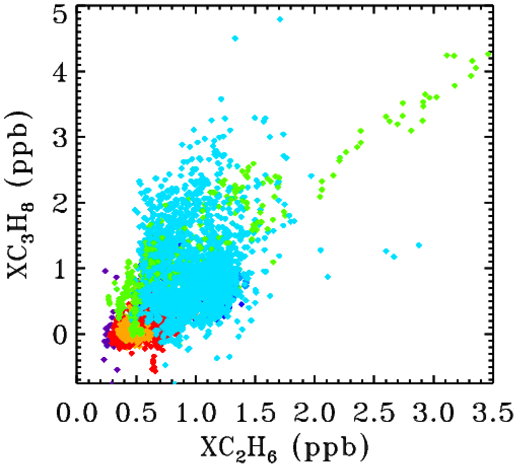
Figure 5 The correlation between XC₂H₆ and XC₃H₈ for all sites, color-coded by site altitude as in Fig. 3.

3.1 Averaging kernels

Figure 6 shows all kernels for the 5000 measurements presented in this paper, color-coded by site altitude (red = 3.8; orange = 2.2; lime green = 1.2; cyan = 0.35; blue <0.2 km) as in the main body of the paper. The kernels increase with altitude but with <40 % variation over the 0–30 km altitude range. Note that the kernels representing the 3.8 km site begin at P=0.7 atm, and the kernels representing the 2.2 km site begin at P=0.8 atm.

Figure 6 The 5000 averaging kernels for C₃H₈ are shown in the left-hand panels ((a), (c)) and those for C₂H₆ are shown in the right-hand panels ((b), (d)). Upper panels ((a), (b)) show all kernels color-coded by site altitude, as in Fig. 3. Lower panels ((c), (d)) show kernels for the low-altitude sites (0.25 to 0.50 km), which were all colored blue in the upper panels ((a) (b)) but are now color-coded by solar zenith angle (blue = 15^∘; green = 60^∘; red = 80^∘).

The lower panel shows the kernels for the low-altitude sites (mainly JPL). These points were all cyan in the upper panel, but in the lower panel they are color-coded by solar zenith angle (SZA). It is evident that the higher the SZA, the more uniform the kernels with altitude. The banding of the points in pressure space reflects the 1 km vertical grid on which the kernels were computed. The C₃H₈ kernels are also influenced by the H₂O column and temperature, but these are smaller effects than those of site altitude or SZA.

Figure 7 show the assumed a priori VMR profile used in the retrievals and in the computation of the kernels. Since GFIT performs profile scaling retrievals, with a very weak a priori constraint, the absolute values of the VMRs play no role; only the profile shape matters.

Figure 7 A priori C₃H₈ profile used in these retrievals.

3.2 Case study: ground-based measurements from Ft. Sumner, New Mexico

Ft. Sumner (34.48^∘ N, 104.22^∘ W; 1.2 km a.s.l.) is the location of the main NASA facility for the launch of stratospheric research balloons. It is located there due to the low population density and hence low risk of mishap. The MkIV instrument has performed balloon campaigns in Ft. Sumner 18 times in the past 30 years. Not all of these campaigns have resulted in a flight, but we have always taken ground-based observations to check that the MkIV instrument is correctly aligned and functional and to check that telemetry, commanding tasks, and the operation of other experiments do not degrade the MkIV performance.

We have taken 520 observations on 106 different days from Ft. Sumner (out of a total of 5000 observations and 1200 different days). We examine these observations to try to understand whether the large day-to-day C₃H₈ variations are real and, if so, what is causing them. We have already seen a correlation between XC₃H₈ and XC₂H₆ at all sites in Fig. 5, but many points are buried under others, especially at the low values of XC₃H₈ and XC₂H₆.

Figure 8 shows that between 1990 and 2005 there was a decrease in C₂H₆ and C₃H₈ measured in Ft. Sumner, by about a factor of 2 over 15 years. In recent years (since 2014), however, there has been a large increase in C₂H₆ and C₃H₈ measured at Ft. Sumner but only when the wind direction is from the SE quadrant (green–cyan colors). We see no increase associated with other wind directions (red, blue, orange, yellow, lime green).

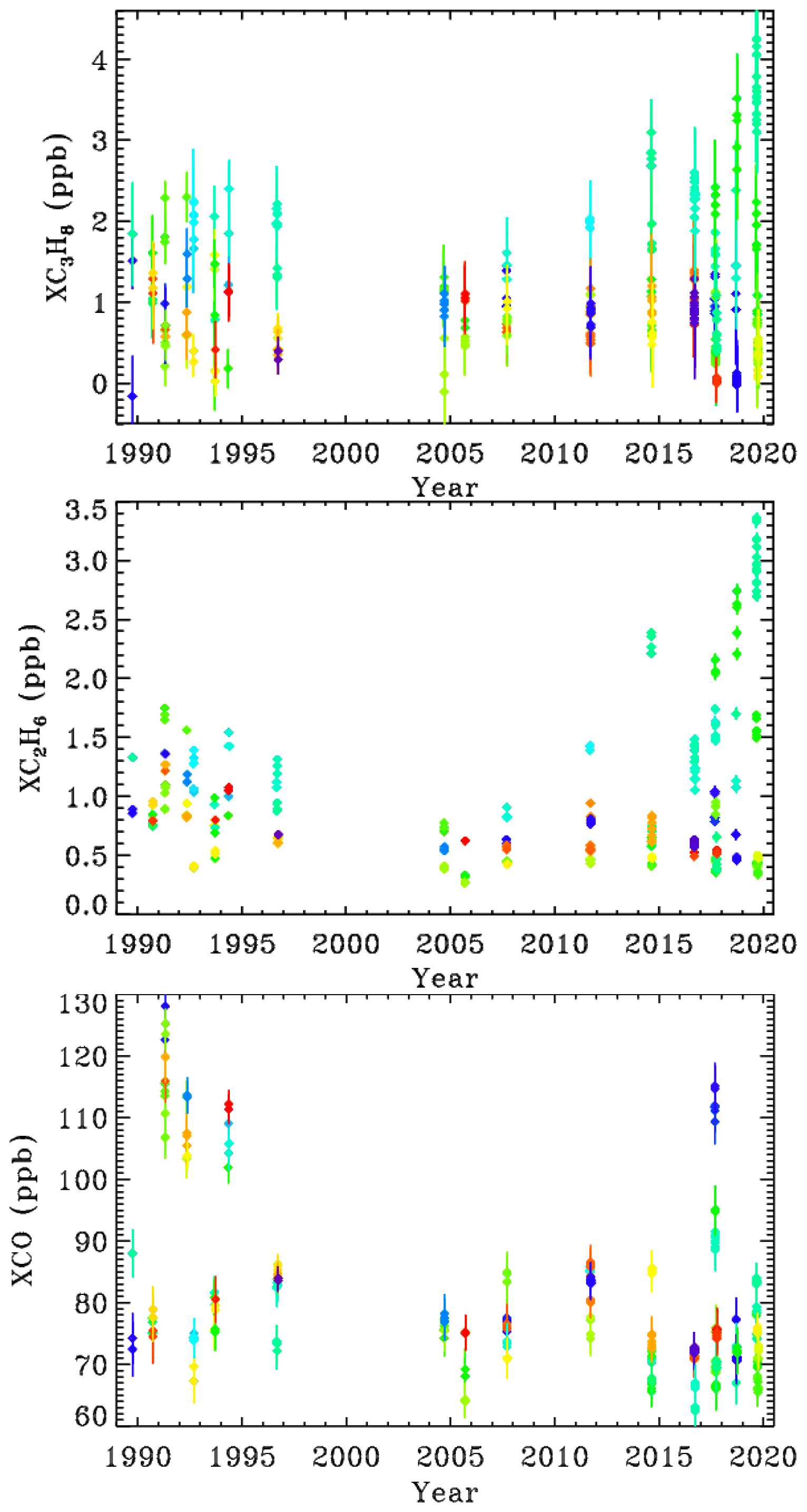
Figure 8 XC₃H₈, XC₂H₆, and XCO at Ft. Sumner. Since all the observations are made from the same altitude, it no longer makes sense to color-code by site altitude. So instead we color-code by mean bearing of the back-trajectory over the previous 36 h. Dark blue = 30^∘; light blue = 90^∘, cyan = 120^∘; green = 180^∘; lime green = 220^∘; orange = 300^∘; red = 350^∘. MkIV did not visit Ft. Sumner from 1997 to 2004, because it was performing high-latitude balloon flights from Alaska and Sweden.

At Ft. Sumner, CO has no correlation with wind direction nor with C₂H₆ or C₃H₈. The majority of days have a column-average CO of 75 ± 10 ppb. But there are occasional enhancements up to 120 ppb, likely due to large but distant fires. We do not pursue the Ft. Sumner CO data any further beyond proving that the C₃H₈ sources are different from those of CO.

CH₄ is also measured by MkIV. Over the 30-year measurement period, XCH₄ has grown from 1650 to 1850 ppb. This secular increase is much larger than any variation due to wind direction. So to be useful, the CH₄ data would have to be detrended, which is not simple given its nonlinear growth. Even within the past 4 years, the correlation of XCH₄ with XC₃H₈ was very weak. This is to be expected since the background abundance of CH₄ is more than 1000 times larger than C₃H₈, whereas wet NG is only 6 times richer in CH₄ than C₃H₈ (in the Permian Basin). So the NG-induced enhancement of CH₄, as a fraction of its atmospheric background level, will be much smaller than that of C₃H₈.

Figure 9 shows a XC₃H₈–XC₂H₆ scatter plot using just the Ft. Sumner data. Error bars are much larger for XC₃H₈ than for XC₂H₆. This is because the C₂H₆ transitions are stronger and form narrower features, both of which make the retrievals more precise and definitive, whereas most of the C₃H₈ absorption is smeared into a broad continuum which provides little information for a retrieval in which the continuum level is fitted. The C₂H₆ features used in the actual C₂H₆ retrieval are at 2976.6 and 2986.6 cm⁻¹ (not shown) and are 3–4 times stronger than those seen in Fig. 2.

Figure 9 The relationship between XC₃H₈ and XC₂H₆ at Ft. Sumner, color coded for wind direction as for Fig. 8.

The gradient of the fitted line is 0.78 ± 0.10, implying more C₃H₈ than C₂H₆. The Pearson correlation coefficient is 0.85, which is high considering the large error bars on the XC₃H₈, and the fact that the similarity of their Jacobians would imply an anticorrelation in their retrieved amounts (Appendix A). This tight relationship at Ft. Sumner suggests that the large variations in the C₃H₈ measurements are not an artifact. Since C₂H₆ can be easily and precisely measured by this technique, it is hard to imagine it being changed by a factor of 5 from day-to-day by an artifact. Much more likely the common variations in both C₃H₈ and C₂H₆ are real.

As already hinted, for each of the 106 observation days from Ft. Sumner, we ran hourly HYSPLIT back-trajectories (Stein et al., 2015; Rolph et al., 2017) that bracket the MkIV observation times and then interpolated linearly in time between the two bracketing trajectories. This provided a unique trajectory for each of the 520 observations from Ft. Sumner. The North American Regional Reanalysis (NARR) meteorology was selected, which covers North America at 32 km resolution. This is the highest-resolution meteorology that covers the entire 1989–2019 observation period. A trajectory altitude of 0.4 km over Ft. Sumner was selected, and these trajectories were extended to 36 h before the observations in 1 h steps. Figure 10 shows that the large variations of C₃H₈ are strongly correlated with wind direction. It is very clear that trajectories originating from the SE of Ft. Sumner carry more C₃H₈ than those from any other direction. A plot was made also for C₂H₆ but not shown due to its strong similarity to Fig. 10.

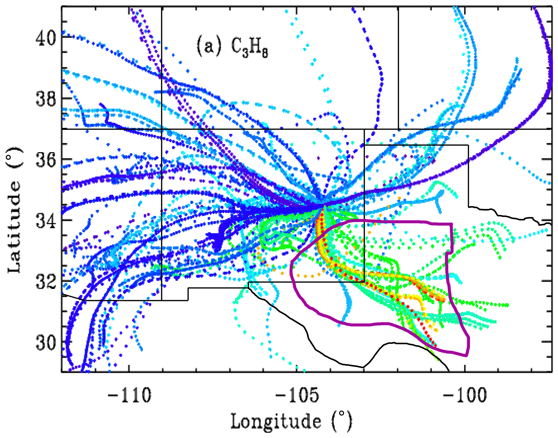
Figure 10 Hourly locations for the back-trajectories, color-coded by retrieved XC₃H₈. Blue = 0, green = 2, red = 4 ppb. Trajectories for which the XC₃H₈ uncertainty exceeded 0.74 ppb are excluded, resulting in only 373 out of 520 trajectories being shown. Ft. Sumner lies at 34.2^∘ N, 104.2^∘ W, which is close to the center of the figure at the confluence of all the back-trajectories. Each point represents a 1 h time step, so the wind speed is apparent from the separation of points. Winds from the west are typically stronger than those from the SE quadrant. Trajectories are underlaid by a map of New Mexico and neighboring states. The Permian Basin, encircled by the thick purple line, underlies SE New Mexico and much of western Texas. Many of the trajectories from the SE have spent more than 30 h over the Permian Basin.

We also made a scatter plot for CO (not shown) but there was no correlation between CO and wind direction or between CO and C₃H₈. This rules out the possibility that the enhanced C₃H₈ and C₂H₆ were somehow associated with distant urban pollution or wild fires.

This result leads to speculation on what might be enhancing C₂H₆ and C₃H₈ when the winds come from the SE sector. One of the biggest natural gas production fields in the US lies in the Permian Basin, which underlies the southeast corner of New Mexico and western Texas, as illustrated in Fig. 10. This region also includes processing plants where the heavier gases are stripped out of the wet NG, storage facilities for the resulting natural gas liquids (LPG + ethane + pentane), and pipelines. The Permian Basin is by far the largest “liquids-rich” (rich in heavy hydrocarbons) gas field in the USA (https://www.spglobal.com/platts/plattscontent/_assets/_images/latest-news/20191219-rig-count.jpg, last access: 20 June 2021). This would suggest that the enhanced C₂H₆ and C₃H₈ are the result of losses from NG production, although this cannot be proven with just one instrument at one site. We would need instruments upwind and downwind to make an accurate assessment of the fluxes.

The Permian Basin currently produces 16 billion cu. ft. per day of NG (https://www.eia.gov/petroleum/drilling/pdf/permian.pdf, last access: 20 June 2021) over an area of 220 000 km². The molar volume of an ideal gas at standard temperature and pressure (STP) is 22.4 L. One cubic foot (cu. ft.) is 28.3 L, so 16 billion cu. ft. is 20 billion moles of NG or 120×10³² molecules per day. Over an area of 220 000 km² or 2.2×10¹⁵ cm², this represents an average areal production of 55×10¹⁷ molecules cm⁻² d⁻¹. Assuming that the Permian Basin is 480 km wide, at an average low-level wind speed of 15 km h⁻¹, an air parcel will take 32 h (1.33 d) to traverse the basin, during which time 73×10¹⁷ molecules cm⁻² will have been extracted. Of this, 10 % will be C₃H₈ (Howard et al., 2015), so if all this production were released into the atmosphere we would expect a C₃H₈ column enhancement of 73×10¹⁶.

In air masses with trajectories from the SE, we see maximum C₃H₈ column enhancements of only 3×10¹⁶ molecules cm⁻², which suggests that only 4 % of the NG escapes into the atmosphere and that 96 % of the NG is successfully captured (or burned by flaring).

In the Permian Basin, NG is 13.7 % C₂H₆, and yet the observed ethane enhancements are slightly smaller than those of C₃H₈, suggesting that only ∼ 3 % of the NG escapes. Assuming a 3 % leak rate, there will also be an enhancement of CH₄ of about 14×10¹⁶ molecules cm⁻², but this represents only 0.4 % of the total CH₄ column above Ft. Sumner and will therefore be difficult to discern in the presence of other confounding factors (stratospheric transport, varying tropopause altitude, seasonal and longer-term changes). Of course, all this analysis assumes that the Permian Basin is a uniform emitter and that the back-trajectory wind speeds are accurate. There are likely hot spots with higher-than-average emissions and regions with little NG production.

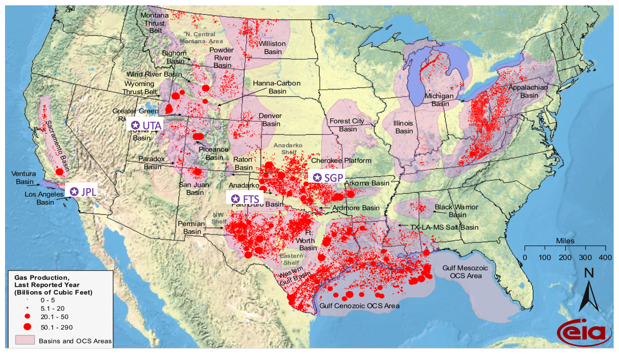
Figure 11 NG production in the lower 48 states of the USA in 2009. Data from the Energy Information Administration: https://www.eia.gov/oil_gas/rpd/conventional_gas.pdf, last access: 20 June 2021. Superimposed are the locations (purple pentangular star) of the four sites discussed in detail in this paper: Ft. Sumner in eastern New Mexico is labeled “FTS”. The JPL site in California is labeled “JPL”. The locations of the NOAA sites in Utah (UTA) and Oklahoma (SGP) are also included. The Permian Basin lies in the SE corner of New Mexico and western Texas.

A puzzle in our findings is that when both C₃H₈ and C₂H₆ are elevated, we measure 22 % more C₃H₈ than C₂H₆ (see Fig. 9). Yet independent assays of well-head wet NG find 33 % more C₂H₆ than C₃H₈ in the Permian Basin (Howard et al., 2015). So we have a 55 % discrepancy. We note that the C₂H₆ averaging kernel is 0.7 at the surface versus 0.9 for C₃H₈ (see Appendix B). So when these gases exceed their priors in the PBL, which is likely at high enhancements, both will be underestimated but C₂H₆ more so than C₃H₈. So this effect would cause the C₃H₈ $/$ C₂H₆ ratio to be 28 % higher, which explains half the 55 % problem. Another possibility is that the C₃H₈ coming from fugitive wet NG is augmented by leaks of LPG, stripped from wet NG. This would further enhance the C₃H₈ (and C₄H₁₀) with little C₂H₆ increase. Alternatively, there could be a systematic overestimate of the MkIV C₃H₈ due to a mundane multiplicative bias in the C₃H₈ spectroscopy. This would overestimate all the C₃H₈ measurements without degrading the strong correlation with C₂H₆ but seems unlikely.

3.3 Case study: ground-based measurements from JPL

The Jet Propulsion Laboratory (34.2^∘ N; 118.17^∘ W; 0.35 km altitude) lies at the northern edge of the Los Angeles (LA) basin. When winds are from the north (rare in summer), air quality is good. When conditions are stagnant (common in summer), pollutants accumulate, and so air quality is poor. C₃H₈ measured at JPL exhibits a very different behavior to that at Ft. Sumner. It decreases over time, exhibits little correlation with C₂H₆, and exhibits positive correlation with CO. Figure 12 illustrates these behaviors.

The left panels of Fig. 12 show XC₃H₈ time series measured from JPL, color coded by CO. The upper-left panel shows a large decrease in C₃H₈ from 1–3 ppb in 1990 to less than 1 ppb in 2019. This mirrors the decrease in CO over JPL (not shown) over the same period. The lower-left panel shows a large seasonal component to the C₃H₈, with a peak in late summer, when the air is most stagnant over JPL, allowing pollutants to accumulate. The highest C₃H₈ values appear red or orange (high CO), while the lowest appear blue (low CO), implying an association with CO. This is confirmed in the upper-right panel which plots C₃H₈ directly against CO. The right panels are color-coded by year. The C₃H₈ correlation is mostly a result of both gases having decreased over the 30-year record. But even within each year, there still remains a positive correlation. This does not necessarily mean that C₃H₈ and CO have the same source, but their sources are spatially coincident.

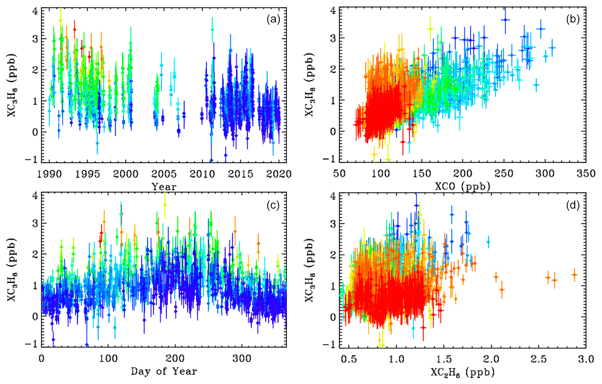
Figure 12 Column-average C₃H₈ above JPL. Left-hand panels ((a, c)) show the time series color-coded by XCO (red = 250, green = 130, blue = 100 ppb). Right-hand panels ((b, d)) show the relationship between XC₃H₈, XCO, and XC₂H₆ color-coded by year (blue = 1990; green = 2005; red = 2019).

The lower-right panel shows C₃H₈ plotted versus C₂H₆. There is a weak correlation at JPL. The high XC₂H₆ values exceeding 2.0 ppb were measured on day 314 of 2015 when JPL was downwind of the Aliso Canyon NG leak. Appendix C shows a HYSPLIT back-trajectory confirming this assertion. This spike can also be seen in Fig. 3. There is no C₃H₈ enhancement associated with the C₂H₆ spike, since processed NG was leaking from an underground storage facility, with the heavy hydrocarbons (e.g., C₃H₈, C₄H₁₀) having already been stripped out. A 2 % increase in column-averaged CH₄ was also noted in the plume of the Aliso Canyon leak, as shown in Appendix C.

California accounts for less than 1 % of total US natural gas production, and this has declined over the past 3 decades (https://www.eia.gov/state/analysis.php?sid=CA, last access: 20 June 2021). Although there is natural gas extraction in the LA basin, this is a small source compared with the Permian Basin. The local natural gas is only 3 % C₂H₆ and 0.3 % C₃H₈, (https://www.socalgas.com/stay-safe/pipeline-and-storage-safety/playa-del-rey-storage-operations, last access: 20 June 2021) and so cannot account for the approximately equal amounts of these gases measured at JPL by the MkIV. We speculate that the C₃H₈ measured at JPL comes mainly from LPG (e.g., used in “clean” commercial vehicles, BBQ grills, external heaters, etc.). We can certainly rule out the possibility that the C₃H₈ measured at JPL is the result of wild fires, since these have increased in recent years, whereas the C₃H₈ has decreased.

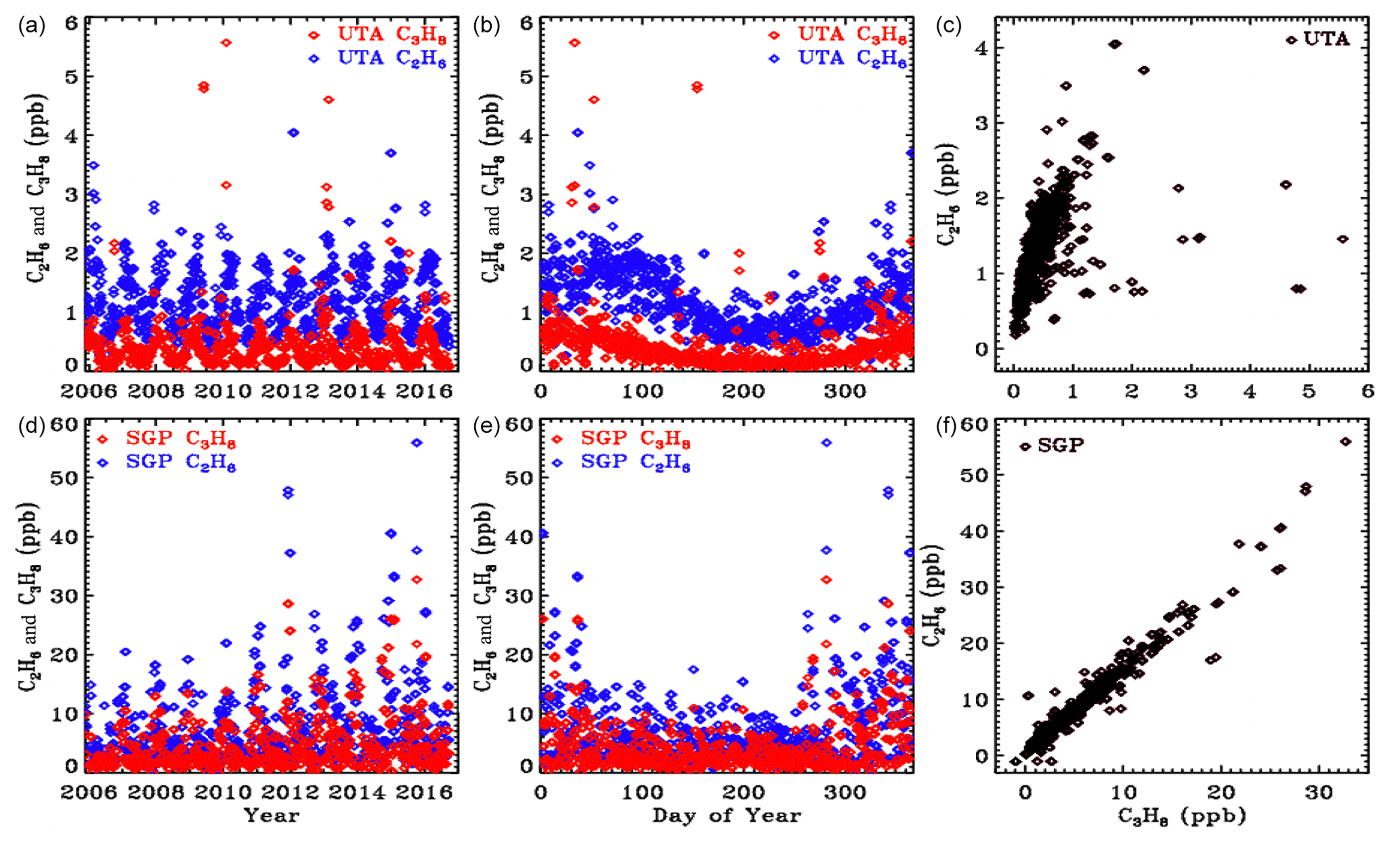
Figure 13 In situ flask measurements of C₃H₈ (red) and C₂H₆ (blue) from the NOAA ESRL GMD dataset (Helmig et al., 2009). Upper panels ((a), (b), (c)) show results from the UTA site. Lower panels ((d), (e), (f)) are from SGP. Note the factor 10 change in the y scale between the two sites. Left-hand panels ((a), (d)) plot data versus year to illustrate secular trends. Middle panels ((b), (e)) plot data versus day of year to more clearly see the seasonal cycle. Right-hand panels ((c), (f)) plot C₃H₈ versus C₂H₆.

3.4 Comparison with in situ measurements

First it should be pointed out that the column-average mole fractions that are derived from the column measurements will underestimate the gas amount in the PBL for gases like C₂H₆ and C₃H₈ that reside mainly in the PBL. For example, if C₃H₈ resides entirely between 1000 and 800 mbar, with none in the free troposphere or stratosphere, then the column-average values will be 5 times smaller than the actual mole fractions in the PBL. So direct comparisons of the remote and in situ mole fractions should be avoided. But their behavior as a function of year or season, or gas-to-gas correlations, can still be meaningfully compared. This effect is in addition to the effect of their averaging kernels being less than 1.0 at the surface, which was discussed earlier.

In situ C₃H₈ and C₂H₆ mole fractions from the Wendover, Utah (UTA), and Southern Great Plains, Oklahoma (SGP), sites were downloaded from the NOAA Global Monitoring Laboratory website: (https://www.esrl.noaa.gov/gmd/dv/data/, last access: 20 June 2021). These sites are the closest to Ft. Sumner. These are surface flask measurements covering the period 2006 to 2017. Figure 13 illustrates these data as a function of the year (left panels), the day of the year (middle panels), and the C₃H₈–C₂H₆ relationship (right panels). The upper panels cover the UTA site and the lower panels the SGP site. Note the factor 10 change in the y scale: there is 10 times more of these gases at SGP than at UTA. Looking at the map in Fig. 11, this is clearly because SGP lies immediately downwind of the Anadarko Basin oil and NG fields under the prevailing WSW winds. In contrast, the UTA site has no major upwind source.

These in situ measurements confirm that C₃H₈ is highly variable with large enhancements being associated with oil and NG production fields. At SGP the C₃H₈ $/$ C₂H₆ ratio is about 0.65. This is smaller than those measured by the MkIV, but NG in the Permian Basin is much wetter (richer in C₃H₈) than in the Anadarko Basin.

3.5 Balloon results

We also attempted to retrieve C₃H₈ from MkIV balloon solar occultation spectra. It was not detected in any flight, despite a very good sensitivity of 0.05 ppb above 5 km. This confirms that the C₃H₈ detected in ground-based measurements, reaching column-average mole fractions of up to 4 ppb, resides mostly in the PBL. The balloon launches are typically performed only under stable, quiescent, meteorological conditions with light surface winds. Such conditions preclude uplift of air from the PBL into the free troposphere, so that C₃H₈ stays confined to the PBL, which is opaque in limb paths due to aerosol and so cannot be probed in occultation. This does not preclude C₃H₈ rising up into the free troposphere at other times or in other places.

4 Summary and conclusions

We report measurements of atmospheric C₃H₈ by solar absorption spectrometry in the strong Q-branch region at 2957 cm⁻¹, using high-resolution IR spectra from the JPL MkIV interferometer. To the best of our knowledge, these are the first remote sensing measurements of atmospheric C₃H₈. The minimum detectable abundance is about 10¹⁶ molecules cm⁻², which is roughly equivalent to a column-average mole fraction of 0.5 ppb. This allows C₃H₈ to be measured in locations where its abundance is enhanced by proximity to sources (e.g., large gas fields, megacities) but not in clean locations (e.g., above the PBL or away from sources). We encourage such NDACC (Network for the Detection of Atmospheric Composition Change) and TCCON sites to examine their datasets for C₃H₈. Future improvements to the spectroscopy of the interfering gases, e.g., H₂O, CH₄, C₂H₆, and other CH-containing gases currently missing, might even provide for the detection of C₃H₈ from clean sites at background levels, allowing it to become a routine product of the NDACC and TCCON networks.

A case study of ground-based MkIV measurements from Ft. Sumner, New Mexico, shows increasing C₃H₈ and C₂H₆ amounts in the past decade on days when back-trajectories came from southeastern New Mexico and western Texas, where the Permian Basin oil and gas field is located. A case study of C₃H₈ measured at JPL shows a long-term decrease since 1990 by more than a factor of 2. It also shows a strong correlation with CO, a tracer of urban pollution. There is no significant correlation between C₃H₈ and C₂H₆ at JPL.

The MkIV measurements in the case studies are not particularly useful for determining the long-term global trends in C₃H₈ or C₂H₆, due to their close proximity to strong sources. In the case of Ft. Sumner, the source is the Permian Basin. In the case of JPL, the source is the Los Angeles urban area with a population of ∼ 15 million. These sources cause large meteorology-driven fluctuations that mask the longer-term trends.

From balloon measurements in solar occultation, propane was analyzed using the same window as for the ground-based measurements. It was not detected at any altitude in any of our 25 flights, despite a 0.05 ppb detection limit. This is presumably because under the stable atmospheric conditions that allow balloon launches, C₃H₈ stays confined to the PBL, which is opaque in the limb viewing geometry and so cannot be probed.

Appendix A: Correlations between retrieved parameters

We compute Pearson correlation coefficients (PCCs) from the a posteriori covariance matrix for each of the 5000 spectral fits. The upper panel of Fig. A1 shows the PCCs between retrieved C₃H₈ and C₂H₆. Points are plotted versus year with the same site-altitude-dependent coloring as in the other figures. The PCCs between C₃H₈ and C₂H₆ averages about −0.7, which means that they are fairly strongly anticorrelated. This is due to their overlapping absorption features at 2967.5 cm⁻¹. So as retrieved C₂H₆ increases, retrieved C₃H₈ will decrease and vice versa. The PCCs are closer to zero for the high-altitude sites (red and orange), presumably due to the reduced pressure broadening and H₂O causing the C₂H₂ and C₂H₆ absorption features to become more distinct. This anticorrelation could be reduced by use of a wider window to introduce additional C₂H₆ features that do not correlate with C₃H₈, but this would also encompass large residuals without adding any C₃H₈ information.

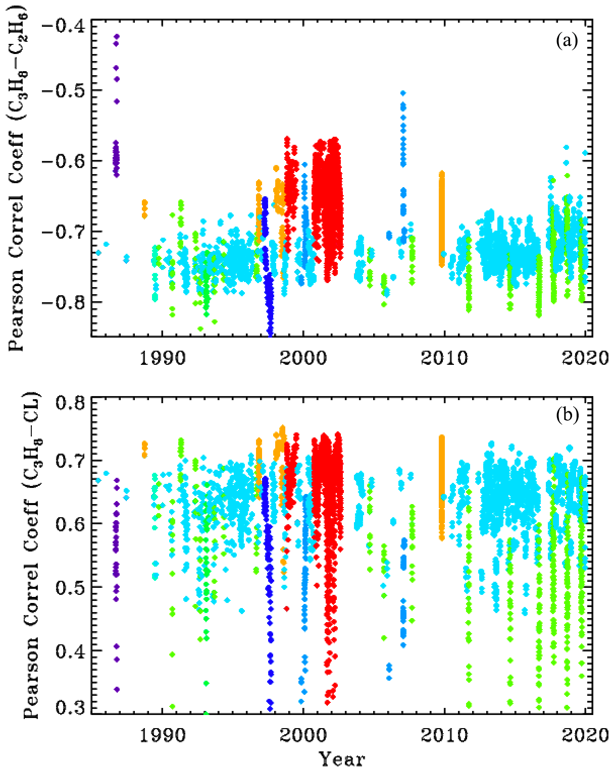
Figure A1 Pearson correlation coefficients between C₃H₈ and C₂H₆ (a) and between C₃H₈ and the continuum level (CL) (b).

The C₃H₈–CL correlations are about +0.65 at low SZA, decreasing at higher SZA as the H₂O and CH₄ absorptions black out the window. So the more C₃H₈ that is retrieved, the higher the continuum level has to be to match the measured spectrum, due to the fact that the C₃H₈ absorption spectrum has a broad continuum-like component beneath the Q-branch. The PCCs between C₃H₈ and the other retrieved parameters (e.g., H₂O, HDO, CH₄, continuum tilt, frequency shifts) were all much closer to zero than with C₂H₆ and CL.

The high PCC between C₃H₈ and C₂H₆ does not necessarily imply a large uncertainty in the C₃H₈. It just means that the large component of the C₂H₆ uncertainty gets projected onto the C₃H₈. Ditto for the CL. But provided the C₂H₆ and CL are well retrieved, their effect on the C₃H₈ will not dominate.

Appendix B: Sensitivity of retrieved C₃H₈ columns to assumed P, T, and H₂O profiles

The retrievals shown in the main body of the paper were performed using 6-hourly NCEP analyses of T, P, and H₂O, as used in the GGG TCCON analyses (Wunch et al., 2011). Due to the overlap of strong H₂O and CH₄ lines with the C₃H₈ Q-branch, we were concerned that small errors in the assumed T $/$ P $/$ H₂O/CH₄ priors might strongly influence the retrieved C₃H₈. We therefore re-retrieved C₃H₈ over the 2000–2020 period using the GEOS-FP-IT 3-hourly analyses, which forms the basis of the latest (GGG2020) TCCON analysis (Laughner et al., 2021). We would have done the entire analysis with the GEOS-FP-IT model except that it only supports the post-2000 time period.

Figure B1 compares the retrieved C₃H₈ columns with the two analysis methods: NCEP in the left panels and GEOS-FP-IT in the right panels. The results look very similar.

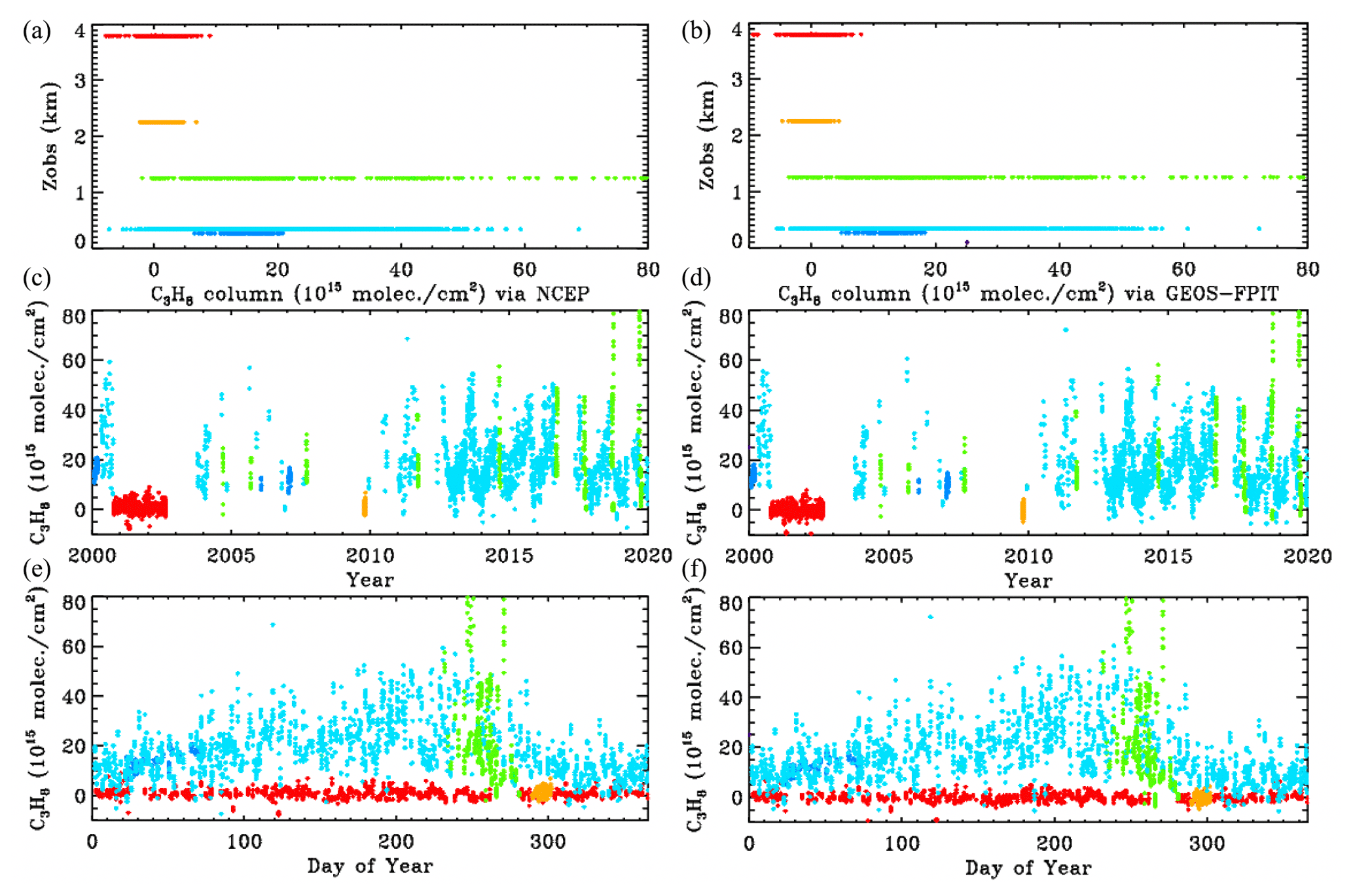
Figure B1 Retrieved vertical columns of C₃H₈ from 2000 to 2020 using two different atmospheric models. (a) NCEP a priori T $/$ P $/$ H₂O. (b) GEOS-FP-IT a priori T $/$ P $/$ H₂O. Points are color-coded by site altitude, as in Fig. 3.

Figure B2 examines more closely the C₃H₈ columns from the two analyses. In the upper panel the NCEP and GEOS-FP-IT columns are plotted against each other. The gradient is 1.011 ± 0.003 with NCEP producing slightly larger columns. The Pearson correlation coefficient is +0.979. The column differences, shown in the lower panel, are mostly less than 5×10¹⁵ and are centered around zero at all column amounts. So the choice of models and priors makes surprisingly little difference to the retrieved C₃H₈. This does not mean that the C₃H₈ is highly accurate. There are many things that are identical in the two analyses (e.g., spectroscopy, retrieval code, spectra), which could nevertheless contribute large errors to the retrieved C₃H₈.

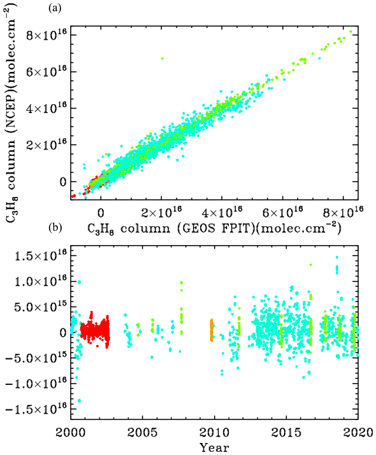
Figure B2 Comparing the C₃H₈ columns retrieved from the 6-hourly NCEP and the 3-hourly GEOS-FP-IT priors, color-coded by site altitude, as in Fig. 3. In the upper panel the columns are plotted against each other. In the lower panel their difference is plotted.

Appendix C: Aliso Canyon underground storage facility: gas leak in late 2015

Aliso Canyon underground storage facility (USF) is located 30 km NW of JPL. According to the 4 January 2016 Los Angeles Times, the NG leak began on 23 October 2015 and peaked on 28 November at 60 t CH₄ h⁻¹. By 22 December, the leak rate had decreased to 30 t h⁻¹ as the underground storage pressure dropped from the initial 2700 psi.

Large C₂H₆ amounts (3 times normal) were observed from JPL on 10 November (day 314) but with no enhancement of C₃H₈. HYSPLIT back-trajectories for this day indicate that the air arriving at JPL at 1000 m above ground was from the northwest and had passed over Aliso Canyon USF, confirming that the air over JPL was contaminated by the leak.

Most of the variation in column CH₄ and N₂O is associated with the stratospheric circulation. Old air masses from high latitudes are depleted in CH₄ and N₂O. To remove these effects and to be able to more clearly see changes driven by the troposphere, XCH₄ is plotted versus XN₂O, which is similarly affected by stratospheric circulation but not by tropospheric emissions. This creates a correlation with the lower-left points representing high-latitude stratospheric air masses and the upper-right low-latitude air masses.

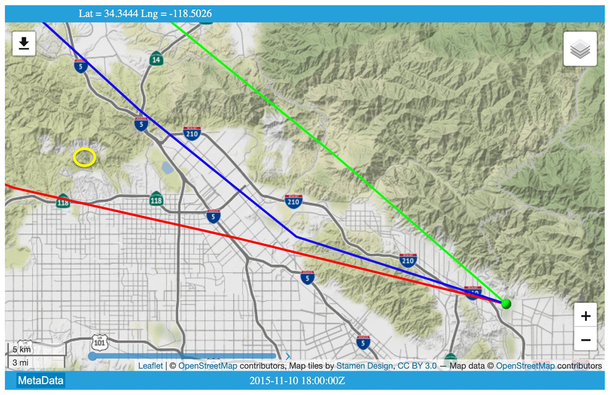
Figure C1 HYSPLIT back-trajectories for 10 November 2015 (day 314) when the highest ever C₂H₆ level was measured from JPL. Yellow oval (upper left) indicates the location of Aliso Canyon underground storage facility. Green ball (lower right) denotes JPL, at the convergence of trajectories arriving at 19:00, 20:00, and 21:00 UT. Trajectory calculation used the North American Model (NAM) 12 km resolution, hybrid sigma-pressure meteorology. © OpenStreetMap contributors 2020. Distributed under a Creative Commons BY-SA License.

Figure C2 Showing the relationship between CH₄ and N₂O at JPL during 2014–2017 color-coded by C₂H₆. Blue points represent low C₂H₆ level, whereas red represents the highest C₂H₆. The encircled points represent 10 November 2015, whose back-trajectory is shown in the previous figure.

The encircled points in Fig. C2 were measured on 10 November 2015, when JPL was downwind of the Aliso Canyon USF leak. This indicates XCH₄ enhancements of over 2 %, which probably represent more than 10 % enhancement in the PBL with no enhancement above. There is also a general tendency for higher CH₄ values when C₂H₆ is elevated on other days too, as seen from the dark blue points (low C₂H₆) being predominantly in the lower right of the figure and the greener points (higher C₂H₆) being located toward the upper left.