3-D tomographic observations of Rossby wave breaking over the North Atlantic during the WISE aircraft campaign in 2017

This paper presents measurements of ozone, water vapour and nitric acid (HNO₃) in the upper troposphere/lower stratosphere (UTLS) over North Atlantic and Europe. The measurements were acquired with the Gimballed Limb Observer for Radiance Imaging of the Atmosphere (GLORIA) during the Wave Driven Isentropic Exchange (WISE) campaign in October 2017. GLORIA is an airborne limb imager capable of acquiring both 2-D data sets (curtains along the flight path) and, when the carrier aircraft is flying around the observed air mass, spatially highly resolved 3-D tomographic data. Here, we present a case study of a Rossby wave (RW) breaking event observed during two subsequent flights 2 d apart. RW breaking is known to steepen tracer gradients and facilitate stratosphere–troposphere exchange (STE). Our measurements reveal complex spatial structures in stratospheric tracers (ozone and nitric acid) with multiple vertically stacked filaments. Backward-trajectory analysis is used to demonstrate that these features are related to several previous Rossby wave breaking events and that the small-scale structure of the UTLS in the Rossby wave breaking region, which is otherwise very hard to observe, can be understood as stirring and mixing of air masses of tropospheric and stratospheric origin. It is also shown that a strong nitric acid enhancement observed just above the tropopause is likely a result of NO_x production by lightning activity. The measurements showed signatures of enhanced mixing between stratospheric and tropospheric air near the polar jet with some transport of water vapour into the stratosphere. Some of the air masses seen in 3-D data were encountered again 2 d later, stretched to very thin filament (horizontal thickness down to 30 km at some altitudes) rich in stratospheric tracers. This repeated measurement allowed us to directly observe and analyse the progress of mixing processes in a thin filament over 2 d. Our results provide direct insight into small-scale dynamics of the UTLS in the Rossby wave breaking region, which is of great importance to understanding STE and poleward transport in the UTLS.

1 Introduction

The upper troposphere and lower stratosphere (UTLS) is the atmospheric region heavily influenced by both stratospheric and tropospheric air masses and is characterised by sharp gradients of many tracer concentrations in both vertical and horizontal directions. The composition of the UTLS plays a key role in stratosphere–troposphere exchange (STE) (Gettelman et al., 2011), and it has a large effect on radiative forcing (Forster and Shine, 1997; Riese et al., 2012) and hence on climate change.

Rossby wave (RW) activity (e.g. Salby, 1984) is one of the major processes that shapes the dynamics and structure of UTLS. In particular, RW breaking is known to steepen the tracer gradients and act as a horizontal transport barrier (McIntyre and Palmer, 1983, 1984) and facilitate STE (Waugh et al., 1994; Günther et al., 2008; Rolf et al., 2015). RW breaking events can transport wet polluted air masses from the troposphere into the lower stratosphere, which is important for the transport of ozone-depleting very short-lived substances and radiatively active substances into the lower stratosphere. The tendency of RW breaking events to create complex spatial distributions of tracers, such as very thin filamentary structures, has been known for some time both from theoretical work (Polvani and Plumb, 1992; Scott and Cammas, 2002) and studies combining modelling with in situ aircraft measurements (e.g. Waugh et al., 1994; Vogel et al., 2011; Konopka and Pan, 2012) or satellite data (Bacmeister et al., 1999; Pan et al., 2009). RW breaking plays an important role in the formation of the extratropical transition layer (ExTL; Shapiro, 1980; Kritz et al., 1991; Hoor et al., 2004), characterised by mixing of tropospheric and stratospheric air masses. Quantifying these mixing processes as well as modelling ExTL structure in general is still a major challenge (e.g. Hegglin et al., 2010). Observing RW breaking, as well as the related mixing and transport, remains difficult: satellite instruments have global coverage but typically lack resolution (vertical resolution in the UTLS is particularly problematic) for the characteristically small scales involved in wave breaking, while in situ observations from aircraft are very highly resolved and accurate, but their spatial coverage is limited to the flight path of the carrier aircraft. Aircraft-based limb sounders provide the very attractive middle ground between satellites and in situ measurements with better resolution than the former and much better spatial coverage than the latter.

In this paper, we present data acquired by the Gimballed Limb Observer for Radiance Imaging of the Atmosphere (GLORIA; Friedl-Vallon et al., 2014), an airborne imaging IR spectrometer. It can be used to retrieve temperature and volume mixing ratios (VMRs) of a number of tracers, including ozone, water vapour, nitric acid (HNO₃), trichlorofluoromethane (CFC-11), chlorine nitrate (ClONO₂) and peroxyacetyl nitrate (PAN), among others. Besides the 2-D slices of the atmosphere acquired by combining a set of atmospheric profiles along the aircraft flight path, GLORIA can be flown around an air volume to acquire a data set suitable for 3-D tomographic retrieval of temperature and trace gas concentrations (Ungermann et al., 2010). 3-D data products have measurement resolution better than 0.2 km vertically and 20 km horizontally. Filamentation and mixing are inherently 3-D processes; their full analysis requires dimensions of features in all spatial directions. These are immediately available when working with 3-D data, while in situ data often involve complex theory or model-based argumentation to compensate for the sparse measurements. Before this study, GLORIA 3-D retrievals were used to study internal gravity waves (Krisch et al., 2017).

The main focus of this case study is to determine to what extent the small-scale tracer structure of UTLS around the polar jet can be understood as a consequence of Rossby wave related stratosphere–troposphere exchange and how this structure is affected by mixing. The outcome of this investigation could further be used to constrain mixing in models as well as to gain insights into STE transport pathways.

The Wave Driven Isentropic Exchange (WISE) measurement campaign took place in Shannon, Ireland, in September–October 2017. A flight on 7 October (Fig. 1a) studied an early stage of a Rossby wave breaking event. Tomographic 3-D GLORIA observations of ozone and nitric acid were performed around a heavily meandered part of the polar jet, resulting in a unique data set with signatures of multiple vertically stacked filaments. The origins of the filaments were studied using backward trajectories computed by the Chemical Lagrangian Model of the Stratosphere (CLaMS; Pommrich et al., 2014). The same air mass was observed again during the subsequent flight on 9 October, in the late stage of the wave breaking event (Fig. 1b). This repeated measurement was used to directly observe mixing in progress by a match of air parcels and comparing the degree of mixing via tracer–tracer correlations. It is also shown that a strong nitric acid enhancement observed just above the tropopause could not have resulted from the descent of stratospheric air masses and is likely a result of NO_x production by lightning activity.

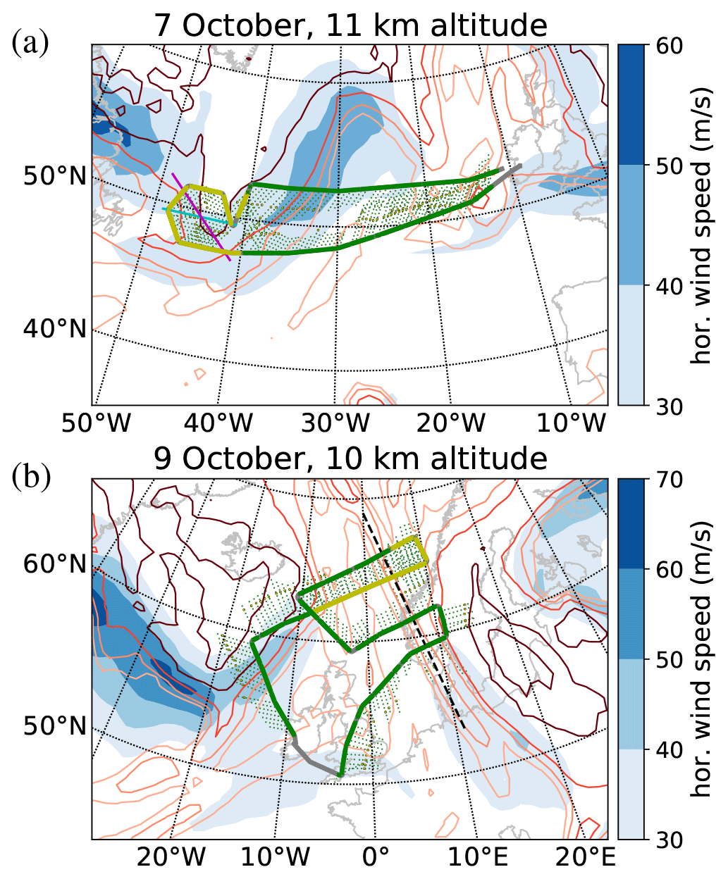
Figure 1 Synoptic situation during measurement flights. Flight track is shown in green for chemistry mode; yellow for dynamics mode measurements. Tangent points are depicted as green dots. Potential vorticity contours for 2, 4, 6 and 8 PVU, respectively, are shown in increasingly darker reddish colours. Magenta and cyan lines in panel (a) mark the position of cuts shown in Fig. 7; the dashed black line in panel (b) marks a filament with older air from the stratosphere (see Sect. 2.2 for discussion).

The paper is organised as follows. Section 2 briefly describes the GLORIA instrument and data analysis techniques as well as the meteorological situation during the two research flights discussed in this paper. Measurement results and analysis of the observed phenomena are presented in Sect. 3. The effects of Rossby wave breaking on the UTLS in the region around the polar jet are discussed in Sect. 3.1 by comparing the vicinity of the jet to surrounding areas in terms of filamentation and tracer correlations. Section 3.2 presents in depth analysis of the small-scale structure observed using 3-D reconstruction within the hexagonal flight pattern of the 7 October flight. Section 3.3 is dedicated to nitric acid–ozone correlation analysis and the origins of the nitric acid enhancement observed just above tropopause. Section 3.4 presents an analysis of the thin filament of stratospheric-tracer-rich air from the 9 October flight and mixing analysis based on air parcels observed during both flights. Finally, conclusions are given in Sect. 4. The appendices provide technical information about data retrieval methods, errors and validation.

2 Measurement and analysis techniques

2.1 GLORIA instrument and retrieval methods

The Gimballed Limb Observer of Air Radiance in the Atmosphere (GLORIA) is an airborne IR limb imager. It is a Michelson interferometer and acquires spectra in the 770 to 1400 cm⁻¹ range (Riese et al., 2005; Friedl-Vallon et al., 2014). Spectral resolution depends on measurement mode. The best possible spectral sampling of 0.0625 cm⁻¹ is achieved in the so-called “chemistry mode” used for retrieving a large number of trace species with often low mixing ratios. One full interferogram is recorded in about 13 s in this mode. In dynamics mode, spectral sampling is reduced to 0.2 cm⁻¹, but the faster acquisition rate of ≈ 5 s per interferogram allows for instrument panning; i.e. the observation direction with respect to aircraft heading alternates between 10 values from 45 to 135^∘. This is useful for observing dynamically complex structures from different directions. The measurements used for 3-D tomography are acquired in this mode.

The detector of the spectrometer is a 2-D array with 128 × 48 effective pixels and 4^∘ × 1.5^∘ field of view in vertical and horizontal directions, respectively. In limb observation geometry, the instrument looks in a close-to-horizontal direction. Infrared radiation along any line of sight comes mostly from the lowest-altitude point on that line of sight (called the “tangent point”). That way, a large range of altitudes can be recorded with the 2-D detector in a single interferogram. This setup also allows for very high vertical resolution of up to 200 m of the retrieved atmospheric quantities. Limb observers can, however, only provide detailed information on the air masses at and below flight altitude. The WISE measurement campaign discussed here was conducted with the German High Altitude and Long Range Research Aircraft (HALO) at flight altitudes up to 15 km. All retrieved data are limited by this altitude.

Best resolution is achieved when the aircraft is flying around the observed air mass in a close-to-circular flight pattern and also panning the instrument (dynamics mode). Due to practical considerations, the actual tomography-optimised flight paths are typically hexagonal and around 400 km in diameter (Ungermann et al., 2010).

Both 2-D and 3-D retrievals are performed by means of inverse modelling, using the Jülich Rapid Spectral Simulation Code version 2 (JURASSIC2). The radiative transfer model (Hoffmann et al., 2008) (employed as the forward model) uses the emissivity growth approximation method (Weinreb and Neuendorffer, 1973; Gordley and Russell, 1981) and the Curtis–Godson approximation (Curtis, 1952; Godson, 1953). The Levenberg–Marquardt algorithm (Marquardt, 1963) and conjugate gradient solver (Hestenes and Stiefel, 1952) are used for inverse modelling. For more information about 3-D tomography implementation, refer to Ungermann et al. (2010, 2011) and Krasauskas et al. (2019). In general, 3-D tomographic retrievals are computationally expensive, typically requiring a few hundred CPU core hours to complete.

The tomographic retrieval combines data from measurements taken over a period of 1 h and 45 min. Some locations are observed from one direction in the beginning of this period and then again from another angle near the end of it. If there is significant change in the measured parameters during that time, these observations will no longer agree. This problem is solved by introducing advection compensation (Ungermann et al., 2011). The main idea of the approach is as follows. We choose a time t_v for which the retrieval will be valid (16:50 UTC in this case, approximately the middle of the measurement time window). As is the case with most instruments, GLORIA retrieval data are provided on a discrete grid. If a measurement was taken at a time t_m, one can relate all required atmospheric parameters (temperature, trace gas concentrations) at each grid point at time t_m to the actual retrieved quantities (atmospheric parameters at time t_v) by advecting grid points at time t_m to time t_v and reinterpolating. In practice, this advection is not performed for every t_m but only for a number of preset values, and then temporal interpolation is used.

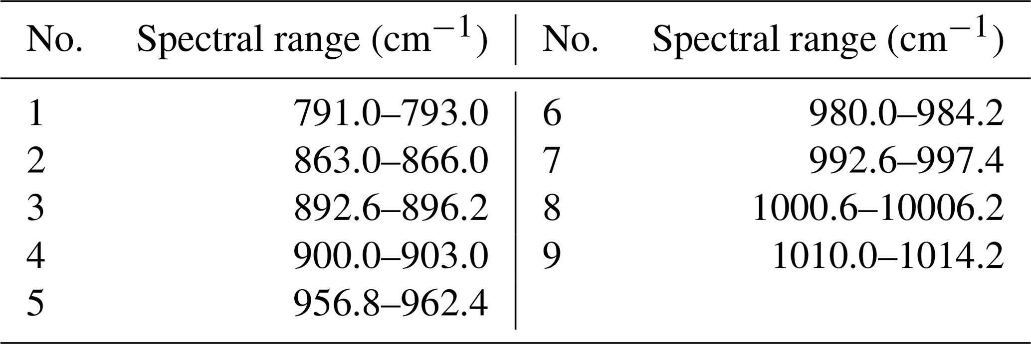
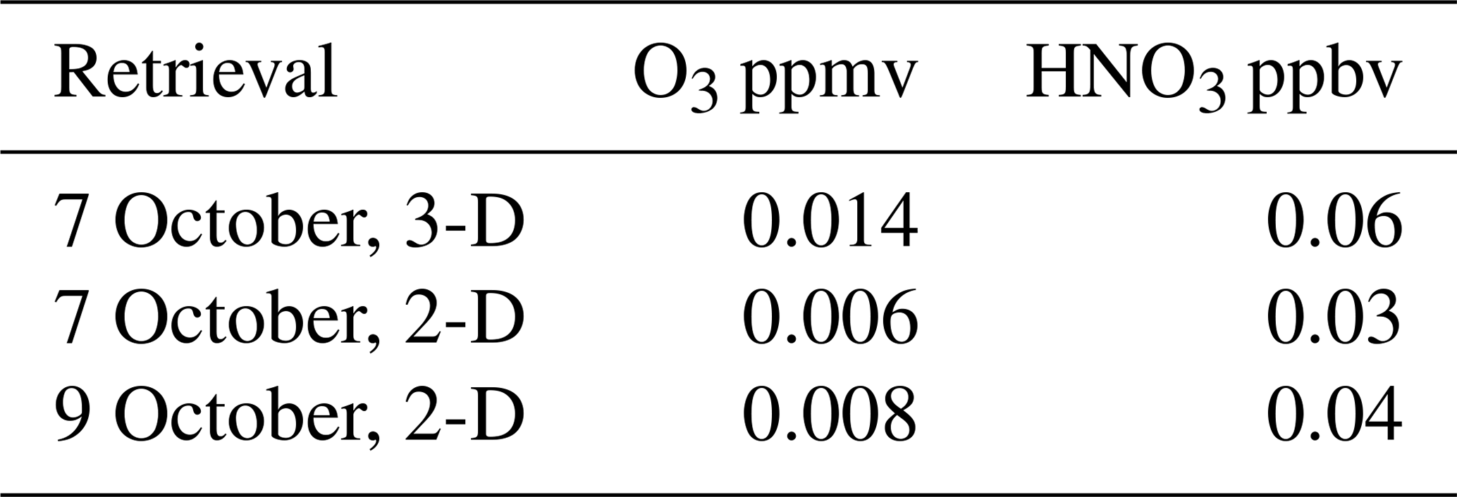
The 3-D retrievals of ozone and nitric acid (HNO₃) shown in this paper were performed using radiances from the spectral windows given in Table 1. The a priori data for air temperature and pressure were taken from the European Centre for Medium-Range Weather Forecasts (ECMWF; Dee et al., 2011) operational analyses. Whole Atmosphere Community Climate Model (WACCM; e.g. Garcia et al., 2007) data were chosen as a priori for ozone and HNO₃.

Table 1 Spectral windows for 3-D retrieval.

2.2 Measurement flights

On 7 October 2017, an onset of a Rossby wave breaking event was predicted over the western part of North Atlantic using ECMWF forecast products. A research flight was planned to probe the UTLS above the polar jet (Fig. 1a). The HALO aircraft took off from Shannon, Ireland, at around 12:30 UTC and landed just after 20:00 UTC. The GLORIA instrument performed well and measured for the whole duration of the flight. These measurements were used for 1-D retrievals, and the resulting profiles were combined into a 2-D data product (curtain) along the flight path.

A hexagonal flight pattern in the Rossby wave breaking region itself was flown between 16:00 and 17:45 UTC, allowing for a 3-D tomographic analysis of the volume. Due to the limited aircraft range, flying a full hexagon this far from the operating base was not possible; hence, only five sides were flown. Also, after flying two of the five sides, HALO climbed from the altitude of 13.4 to around 13.9 km. For best results and easier processing, one would wish to avoid climbing in the middle of the tomographic data acquisition. In this case, however, flying at the higher altitude was not possible earlier due to the weight of the remaining fuel. Also the benefits of flying the last three hexagon sides higher and hence observing a wider altitude range were deemed more important. This choice was further motivated by the presence of optically thick clouds at low altitudes. In parts of the hexagon, cloud tops reached to almost 10.5 km altitude, thereby restricting the altitude range available for retrieval. Another complication for producing 3-D data was the high wind speeds of the polar jet, reaching more than 40 m s⁻¹, resulting in significant advection of air masses during the measurement acquisition time (see Sect. 2.1 for a solution to this particular problem). The measured air masses could be successfully reconstructed in 3-D despite these challenges. The tomographic retrieval is complemented by 2-D data (curtains of profiles obtained from 1-D retrievals) of the region immediately east of the hexagon, which also proved to be of interest.

By 9 October 2017, the wave breaking event was at its final stage and most of the air masses that were present in the hexagon flown 2 d before were stretched into a thin filament extending from 70^∘ N, 0^∘ E, to 51^∘ N, 12^∘ E. This filament can be seen as an elongated 2 PVU contour in Fig. 1b and is highlighted by a dashed black line. A research flight on 9 October was flown to investigate the late stage of this RW breaking by measuring this filament. The aircraft crossed the filament a total of four times during this flight, as seen in Fig. 1b. The flight lasted from 08:30 to 17:00 UTC. In this paper, we present only 2-D data products from this flight.

2.3 Backward trajectories

Backward-trajectory calculations from CLaMS (Pommrich et al., 2014) were used for measurement data analysis. CLaMS back-trajectory calculations are very well suited to analyse the detailed transport pathway of an air parcel in the UTLS and were applied to a variety of problems such as transport in the tropics as well as STE processes (e.g. Ploeger et al., 2012; Vogel et al., 2014; Li et al., 2018). The model was driven by winds obtained from ECMWF operational analysis data. An air parcel was placed at each grid point of the GLORIA data product, and the trajectories of these parcels were traced back for up to 1 month. Mixing and chemical processes, which are normally included in the 3-D version of CLaMS model, are not used for backward-trajectory calculations. One of the main uses of backward trajectories was to determine the stratosphere residence time of the observed air parcels. The maximum potential vorticity gradient tropopause (Kunz et al., 2011) was used to define stratospheric and tropospheric regions along the calculated backward trajectories. This tropopause definition is based on the product of isentropic PV gradients and wind speed. It is well suited for our study, as it is generally in good agreement with chemical discontinuity in trace gas distributions.

3 Results and discussion

3.1 Filamentation and mixing near and away from the polar jet

The results presented in this section are based on the GLORIA 2-D data products. They were generated along most parts of both flights considered in this work (Fig. 1). The measured volume mixing ratios of ozone, water vapour and nitric acid for the 7 October flight are presented in Fig. 2. The retrieved values are shown as functions of time and altitude, but it is important to remember that the GLORIA 2-D curtains do not represent a vertical cut through the atmosphere along the flight path but a slant curtain. At flight altitude, the data shown represent the atmosphere ∼10 km to the right of the aircraft, while at lowest altitude this distance increases to up to 250 km. The locations of the tangent points of the observations are shown in Fig. 1a. The missing data in Fig. 2 are due to aircraft manoeuvres and optically thick clouds. In the cases where clouds are present, atmospheric properties can only be retrieved in the regions above cloud tops. The retrieval of 2-D data was also performed for the hexagonal part of the flight path (from 16:15 to 17:42 UTC) for consistency, even though the 3-D data were available for that part of the flight. 2-D data products are valid at the measurement acquisition time indicated in the plots.

Figure 2 (a–c) 7 October H₂O, O₃ and HNO₃ 2-D GLORIA data along the flight path in Fig. 1a. (d) Stratosphere residence time (yellow for ≥30 d). Isentropes – dashed lines; 2 and 4 PVU contours – thick solid lines; thermal tropopause – dots.

Generally, water vapour has high volume mixing ratios in the extratropical troposphere and is much less abundant in the stratosphere due to freeze-out in particular around the tropical tropopause (e.g. Schiller et al., 2009). O₃ and HNO₃ are more abundant in the stratosphere, where their abundances are controlled by photochemistry, and less abundant in the troposphere. Generally, these two gases have a compact positive correlation in the deep stratosphere. The correlation is attributed mostly to source and sink regions being similar for the two gases and not a result of chemical interactions between them (Sect. 3.3; Popp et al., 2009). Retrievals generally confirm this generally expected behaviour but also show heavily filamented structures in all the tracers presented here. There is a clear positive correlation between ozone and nitric acid: ozone-rich air masses tend to have high nitric acid concentrations, and vice versa. One can also see negative correlation between water vapour and ozone (or, alternatively, between water vapour and nitric acid), especially around 16:15 and 18:30 UTC, where the H₂O structure shows more filamentation. This suggests that the whole structure was formed by STE: air parcels rich in ozone and nitric acid (old air) come from higher up in the stratosphere, while wet air masses have relatively recently resided in the troposphere (young air).

The origins of the filaments were investigated using CLaMS backward-trajectory calculations. The typical mix-down timescale (i.e. time needed for the mixing to erase all structure) for the Rossby wave surf zone in the lower stratosphere is of the order of 1 month (Juckes and McIntyre, 1987). Hence, in this region, one may expect small-scale ozone-poor structures to be a consequence of transport of ozone-poor tropospheric air across the dynamical tropopause within the last month. Based on this reasoning, we plotted the air parcel residence time in the stratosphere (i.e. time spent above the maximum potential vorticity gradient tropopause) of each stratospheric air parcel observed by GLORIA (Fig. 2d). There is good agreement between young air masses in Fig. 2d and ozone-poor and HNO₃-poor air in GLORIA retrieval (Fig. 2b, c). Almost all ozone-rich (>0.25 ppmv) air masses, including thin filaments, have stayed in the stratosphere for more than 1 month. Younger air, conversely, is almost always ozone poor. Also, wet air filaments correspond to young air masses from the troposphere that can be seen best around 16:15 UTC, 10–13 km altitude; 17:50 UTC, 11.5 km altitude and 18:40 UTC, 13–14 km altitude. Unfortunately, the air mass within the hexagonal flight pattern (16:15 to 17:42 UTC) was very dry; significant water vapour structures could only be found around the very edges of the hexagon and were advected outwards while this pattern was flown. The 3-D tomographic water vapour retrieval was therefore not performed.

HALO took off from Ireland, which was, at the time of the flight (7 October), south of the polar jet and therefore not directly affected by air masses of the polar UTLS, the polar jet and Rossby waves that shape it. One can clearly see the jet (in wind speed) and Rossby waves (in PV) in Fig. 1a. Conversely, the western part of the flight, including the hexagonal flight pattern, is directly on top of the polar jet and therefore heavily influenced by it and the RW surf zone. To illustrate this difference, we divided the observed air masses into those “near polar jet” (we defined these as air masses observed at locations west of 30^∘ W and with PV > 1 PVU at 11 km altitude) and “away from the jet” (all the rest). The locations of observation for these air masses are shown in yellow and orange, respectively, in Fig. 3. The PV at 11 km is plotted there as well and shows Rossby waves. The polar jet is located on the edges of the high-PV area (see Fig. 1). The backward-trajectory calculations show the position of the observed air parcels 3 d before observation. We see that the air masses “away from the jet” (black) came from lower latitudes and did not travel as far around the pole. The air found near the jet (red) has stayed near the jet for the last 3 d at least. The air parcels measured on 7 October as a rather compact group were stretched through a long portion of polar jet on the other side of the pole just 3 d ago. These air masses were brought together by strong wind shear and subsequently transported far away by the strong westerlies of the jet. Note as well that the original positions of “near-jet” air look especially dispersed around a breaking Rossby wave at 140^∘ W. Such a sparse group of air parcels could only be brought into a compact group by strong wind shear and stirring in the breaking RW. This difference in air mass origin explains why most of the filamentation in trace gas structure can be seen between 15:10 and 19:10 UTC (“near-jet” air). The origins of air inside the hexagonal flight pattern will be studied in more detail in Sect. 3.2.

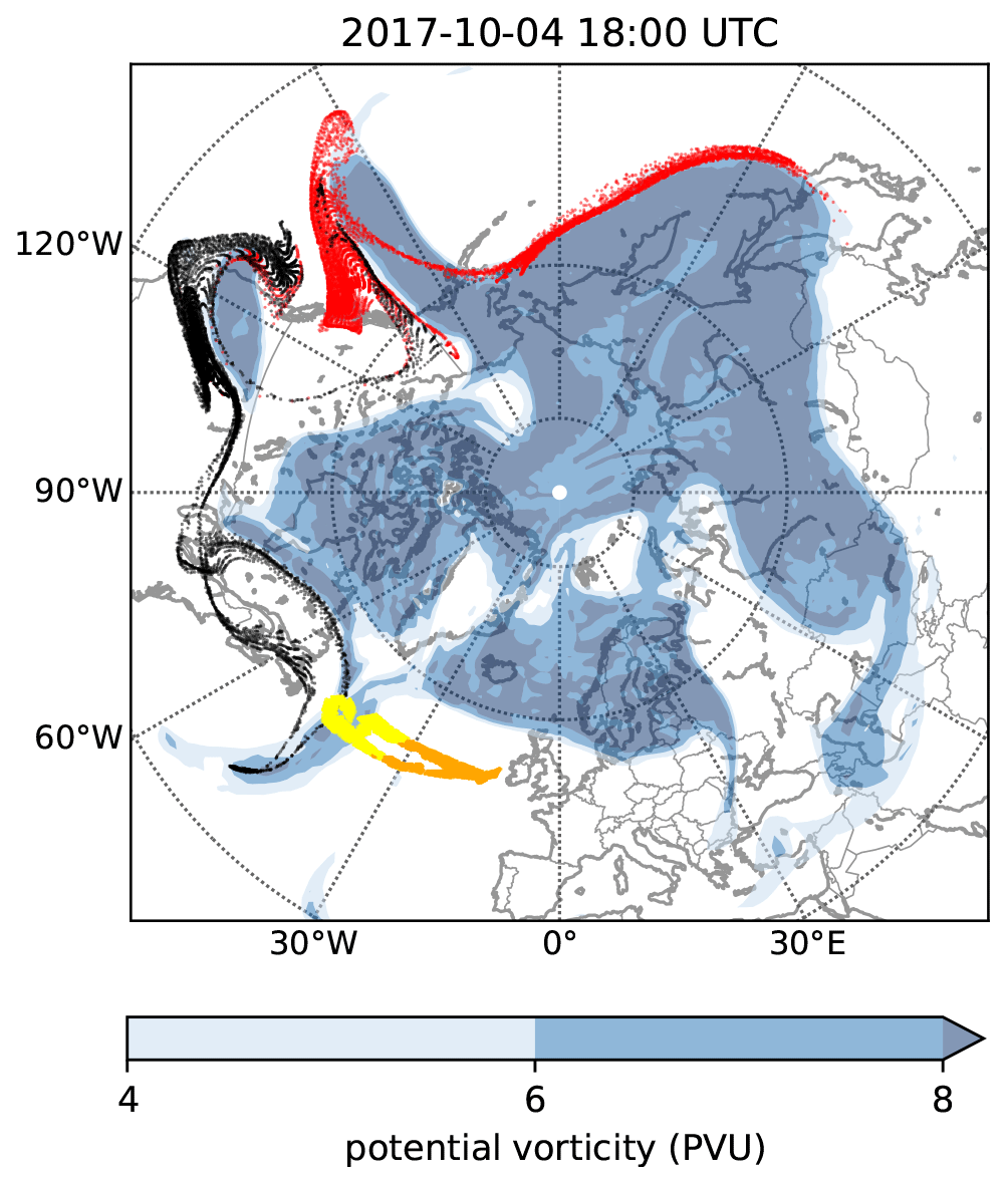
Figure 3 Air mass origin plot for the retrieved 2-D data. Horizontal cut at 11 km altitude 3 d before measurement flight is shown. Locations of GLORIA observations on 7 October: yellow – near polar jet (west from 30^∘ W, PV > 1 PVU); orange – away from jet (all the rest). The positions of “yellow” air parcels 3 d before measurement are shown in red; those of “orange” air parcels are in black.

To highlight the effect of RW breaking, we provide separate O₃–H₂O tracer–tracer plots for near-jet air masses (Fig. 4a) and the rest (Fig. 4b). We designate air parcels as stratospheric if they contain less than 10 ppm water vapour and tropospheric if they have less than 0.1 ppm ozone. Air parcels that fall into neither of these two categories are typically products of mixing between stratospheric and tropospheric air (Proffitt et al., 1990; Hoor et al., 2002; Pan et al., 2004). When compared to in situ measurements, GLORIA data have lower spatial resolution, making it more difficult to identify individual mixing lines, but they have better spatial coverage, allowing us to see a more complete picture of mixing across a range of altitudes. In the eastern part of the flight, there is evidence of some mixing but only between end members with relatively low values of both ozone and water vapour. This indicates that stratospheric air masses do not penetrate far into the troposphere, and vice versa. Since in situ observations represent a more spatially limited data set (black dots), two separate mixing lines can be discerned there. The “western” part of the flight, close to the polar jet, shows evidence of more vigorous mixing. The air mass with around 0.2 ppmv O₃ and 30 ppmv H₂O could only have originated from a substantially deeper STE than that needed to explain the ozone–water vapour structure of the eastern part of the flight. As the aircraft stayed in the stratosphere for the whole western part of the flight, all in situ data show stratospheric signatures.

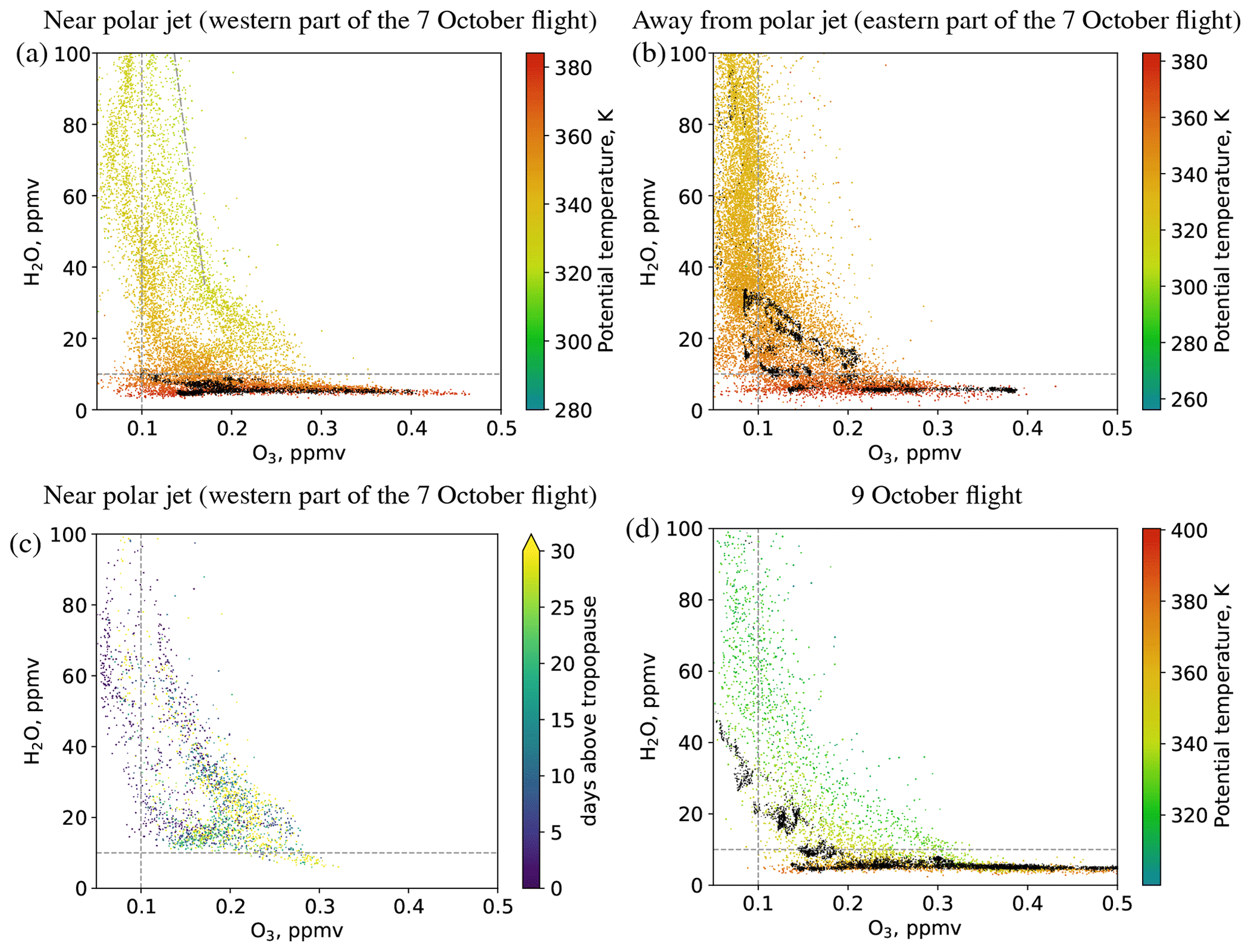
Figure 4 Ozone–water vapour tracer–tracer correlations. Black dots represent in situ measurements at flight altitude. O₃ was measured by FAIRO (Zahn et al., 2012); H₂O – by FISH (Meyer et al., 2015). The dashed grey lines mark 0.1 and 10 ppmv values of ozone and water vapour, respectively, as discussed in the main text. In panels (a, b, d), GLORIA measurements are colour coded in potential temperature. In panel (c), only stratospheric air parcels below θ=350 K are shown; all stratosphere residence times greater than or equal to 30 d are depicted in the same colour.

A particularly interesting feature in the western part of the flight is a distinct branch of wet (>20 ppmv water) air with potential temperatures consistent with the upper troposphere in this region and enhanced ozone (>0.15 ppmv), suggesting an influx of stratospheric (or partially mixed with stratospheric) air into relatively low levels and intense mixing. This feature was studied in detail using backward trajectories. Figure 4c shows the stratosphere residence time for all air parcels observed in the stratosphere below 350 K potential temperature level during the western part of the flight. Firstly, it is notable that majority of the air observed in this region seems to be mixed to some degree. This is evident both from the general position of air parcels in tracer–tracer space and the strong variation of stratosphere residence times within the tracer–tracer space structures, suggesting different origins. Also, points with more than 40 ppmv water and more than 10 ppmv ozone seem to be arranged in mixing lines. The line highlighted in Fig. 4a appeared in the observations between 18:15 and 18:25 UTC (a 160 km long flight stretch). All measurements from that part of the flight below 330 K potential temperature and below 150 ppmv water vapour are shown in Fig. 5a. This correlation suggests that an air mass with stratospheric residence times above 10 d and water vapour below 40 ppmv, which was itself a result of earlier mixing, descended close to the tropopause and became the more stratospheric end member for another mixing event with wet air of the upper troposphere. This is supported both by the very different stratosphere residence times of this air mass to the rest of the mixing line and the fact that the line lacks clear extension into lower water vapour values (see Fig. 4a). Figure 5 shows the backward trajectories for this “more stratospheric end member” (blue lines) and the rest of the mixing line (defined by water vapour between 40 and 100 ppmv, orange lines). The trajectories indicate that the more stratospheric air parcels were advected as a very tight group since a Rossby wave breaking (RWB) event 8 d before the measurement brought them together, the group had not been as tight at earlier times. Some of these parcels come from higher up in the stratosphere, some from the planetary boundary layer (PBL) as recently 20 d before our measurement, but the group seems to be well mixed at the time of measurement. The rest of mixing line was only brought together during the RWB event 3 d before measurement and the mixing was clearly ongoing when observed. These results could be used to roughly constrain the mixing time scale in this region of UTLS. A more detailed analysis, using mixing schemes in the numerical models, would be required to give tighter, more robust bounds and to account for possible differences in wind shear or for influence of air masses not observed by GLORIA. However, our results seem to indicate that 8 d were enough for mixing to run its course, while 3 d were not.

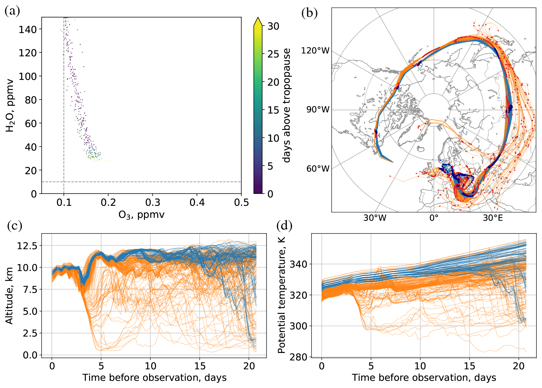
Figure 5 Panel (a) shows ozone–water vapour tracer–tracer correlation for 7 October flight below 330 K potential temperature. Colour scale shows stratosphere residence time; tropospheric air parcels are included with zero residence time. The remaining panels show backward trajectories for air parcels from (a) air with less than 40 ppmv H₂O and residence time above 10 d (blue), and air with 40 to 100 ppmv H₂O (orange). Trajectories in panel (b) have markers every 24 h (red for orange trajectories; dark blue for blue) and are plotted for 10 d in total.

The O₃–H₂O correlation for the 9 October flight (Fig. 4d) has a line indicating deeper mixing than the rest of the flight and similar to the line in the 7 October flight we discussed in the previous paragraph (Fig. 4a). This is not surprising and supports the previous result, since many of the air masses seen during the 9 October flight come from the area observed on 7 October around the hexagonal flight pattern. The relative lack of purely tropospheric air masses is due to high clouds that prevented measurements in the troposphere (see Sect. 3.4 and Fig. 13).

The combinations of ozone and water vapour concentrations observed by GLORIA during this flight are generally compatible with in situ observations during previous campaigns. For example, the air parcels indicating intense mixing, like the ones with 0.27 ppmv O₃, 20 ppmv H₂O or 0.2 ppmv O₃, 50 ppmv H₂O are within the range of values observed near Fairbanks, Alaska, during the POLARIS campaign in 1997 (Pan et al., 2009).

3.2 3-D tomography of filamentation near the polar jet

In this section, we study the origin of the air inside the hexagonal tomographic flight pattern on 7 October (see Fig. 1a). The flight pattern is shown, together with a 3-D plot of ozone results, in Fig. 6. The results of the tomographic retrieval for ozone and nitric acid (HNO₃) are presented in detail as vertical 2-D cuts through the measured volume in Fig. 7. There is, as before, a clear positive correlation between the two trace gases. A more detailed look into this correlation is presented in Sect. 3.3.

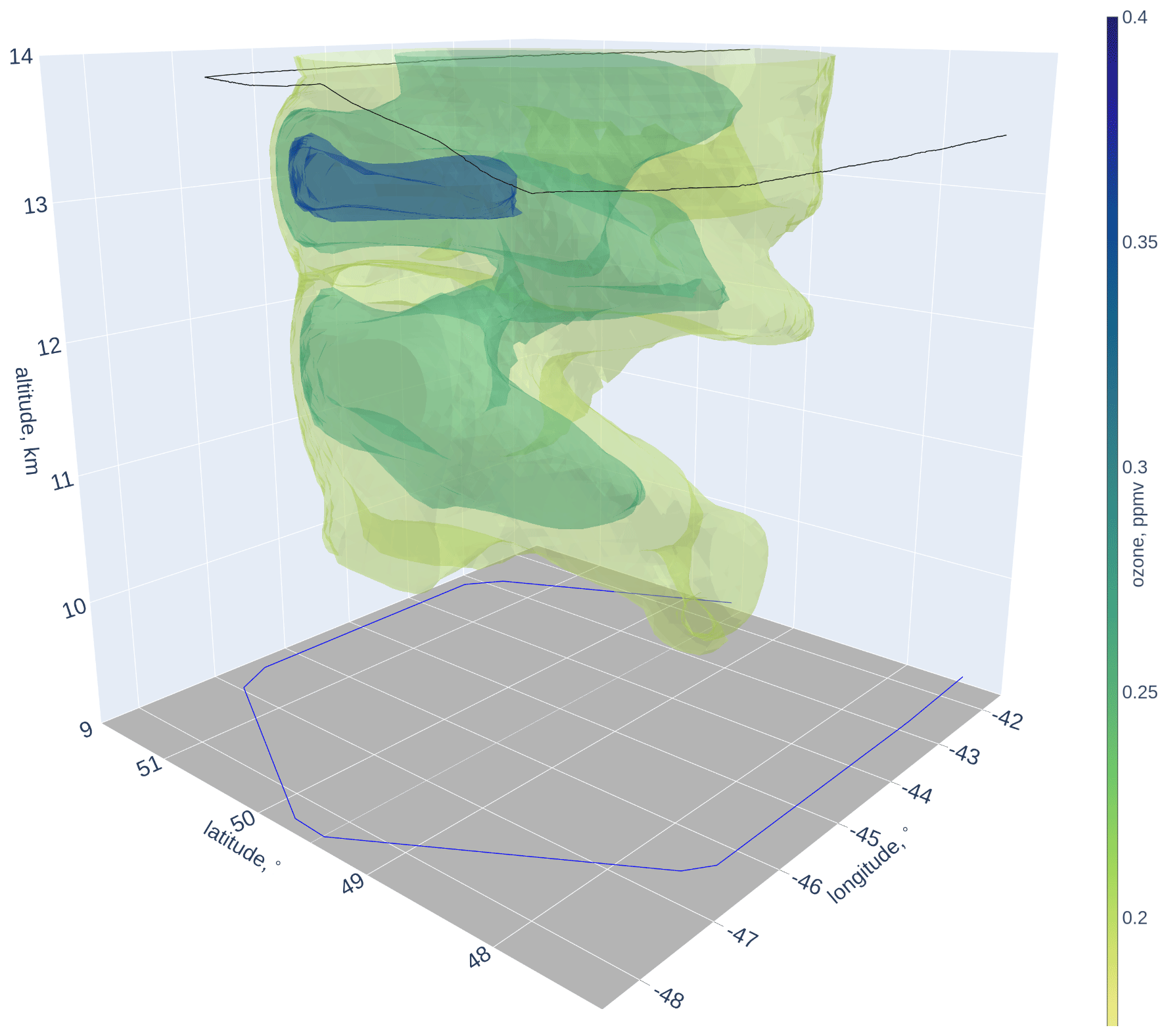
Figure 6 3-D plot of tomographic retrieval of ozone VMR. The flight track is represented by a thin black line; a horizontal projection of the flight track is represented by a thin blue line.

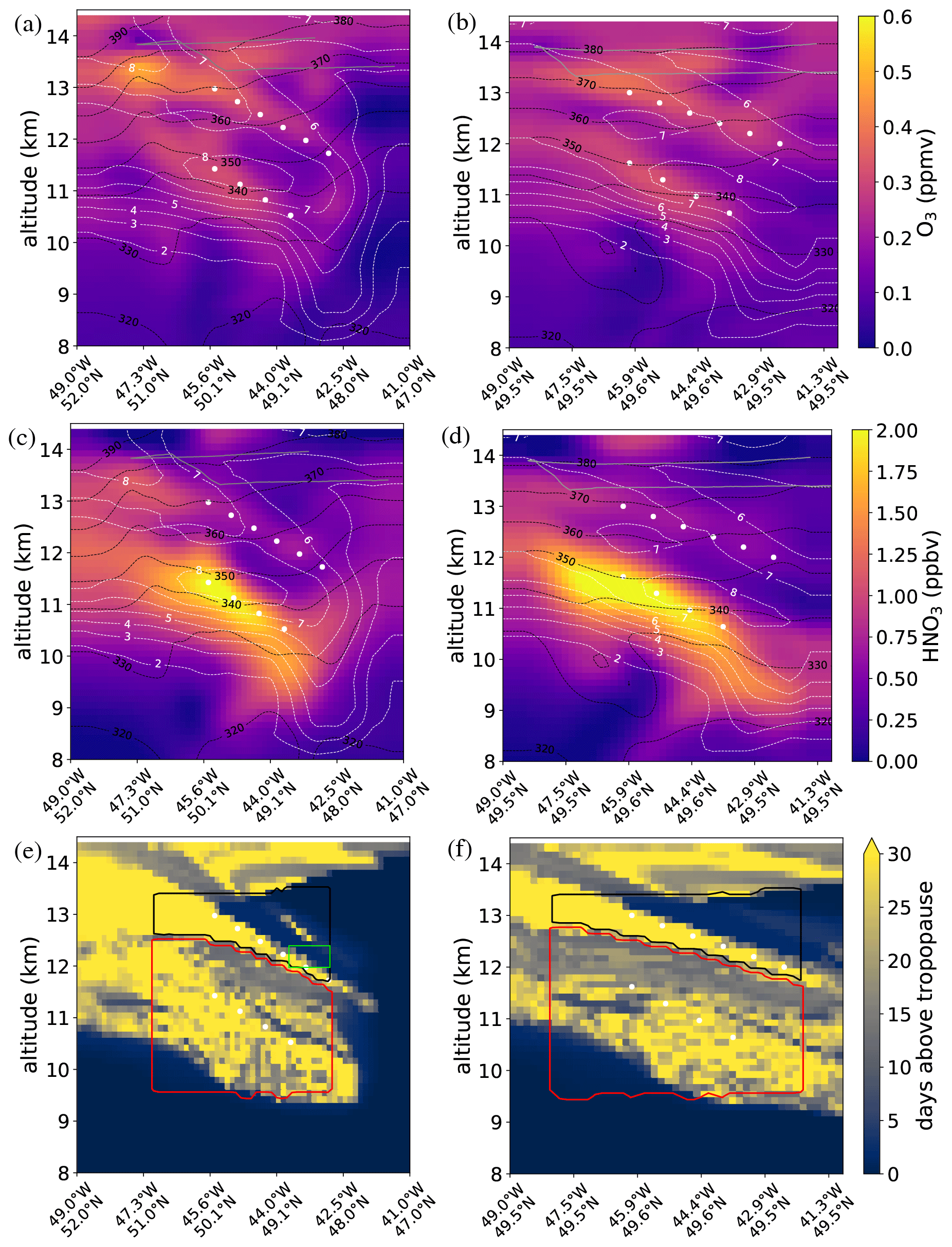
Figure 7 Panels (a–d) show vertical cuts through 3-D tomographic retrieval and corresponding air mass origin plots. The solid grey line shows the projection of flight path onto the displayed cut; dashed black lines indicate isentropes, labelled in K; dashed white lines indicate PV isosurfaces, labelled in PVU. Panels (e–f) show air residence time in the stratosphere; black and red lines show the position of air parcels for which backward trajectories were calculated. Their previous positions are depicted, with those same colours, in Fig. 8. Positions of vertical cuts are shown in Fig. 1a: left panels – magenta; right panels – cyan. White dots mark filaments (see Sect. 3.2).

Figure 7 also shows a complex structure of thin filaments (layers) of younger and older air in the lower stratosphere (LS). As in the previous section, we use backward trajectories to determine the “age” (time spent above dynamical tropopause) of each stratospheric air parcel observed by GLORIA (Fig. 7e, f). The two older air filaments (marked with white dots) that are the main features of both ozone and nitric acid retrievals can be identified with the two filaments of air that have stayed in the stratosphere for more than 30 d. Younger air masses can be seen in between the two filaments as well as above them. The boundary between older stratospheric air and the troposphere at 10–11 km altitudes is also reflected in the retrieval. For ozone, in particular, values higher than approximately 0.25 ppmv within the hexagonal flight pattern are mostly measured for air parcels that stayed in the stratosphere for more than 30 d. The accuracy and resolution of the retrieval decreases away from the centre of the hexagonal flight pattern, which is the likely reason for the “smearing out” of the filaments at around 48^∘ N, 42.5^∘ W.

The panels of Fig. 7 with GLORIA data also show potential temperature isolines, derived from GLORIA temperature retrieval and ECMWF pressure data. The major filaments are almost uniform in nitric acid and especially ozone structure, despite the fact that they are not isentropic. This suggests that diabatic processes or turbulence due to Rossby wave breaking were involved in their formation. The arrangement of tracer filaments and potential vorticity with respect to potential temperature surfaces shows that scale breakdown has occurred: although the filaments remain quasi-horizontal, they can subsequently be erased by mixing along isentropes, making the effective horizontal length scales shorter (≈100 km around the upper filament).

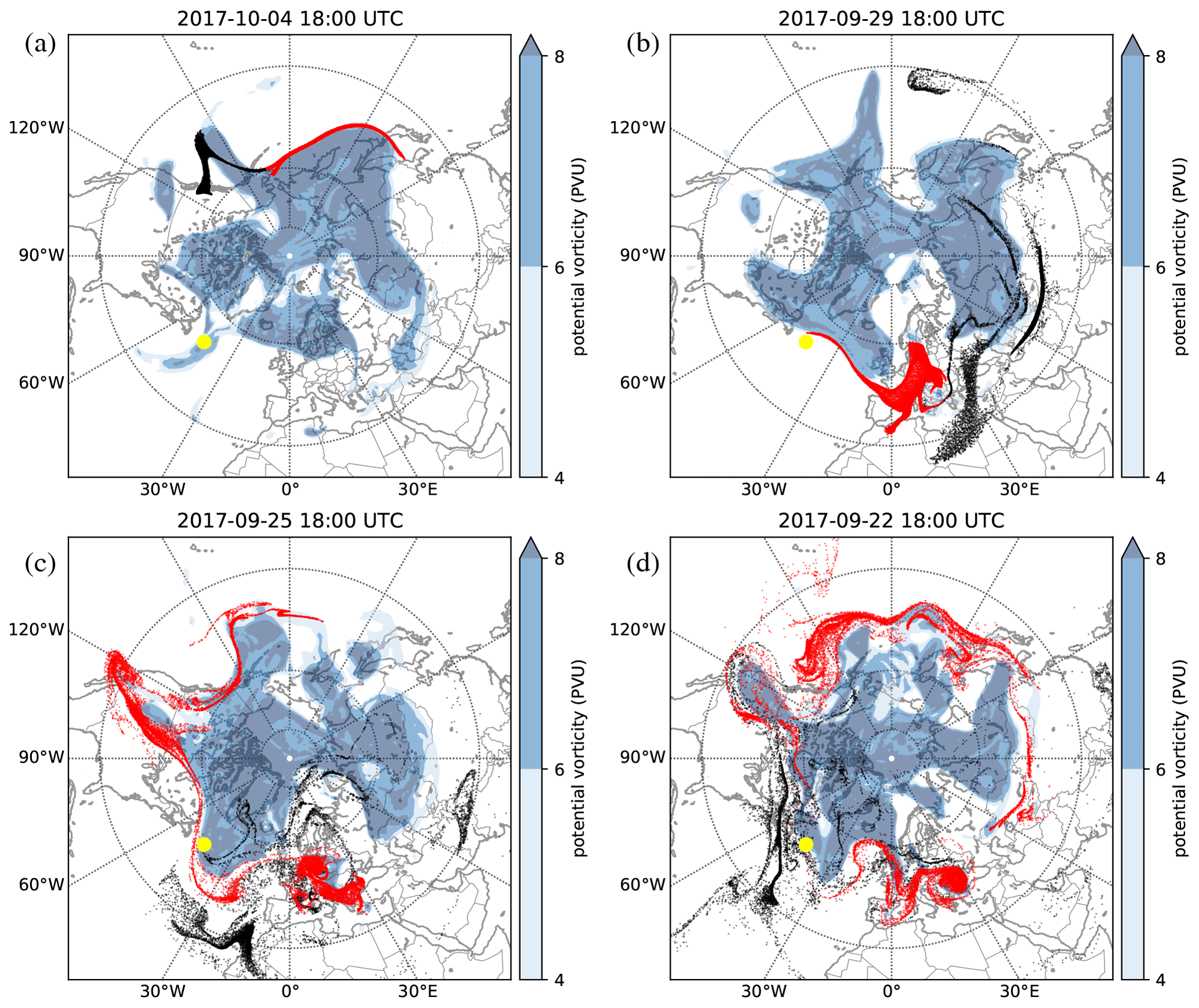
Figure 8 Origins of observed air parcels. Panels show horizontal cuts at 11 km altitude. Potential vorticity is shown in shades of blue. The location where air parcels were observed by means of GLORIA 3-D tomography on 7 October is shown in yellow (they form a small disc). The parcel locations at the dates indicated for each panel are shown in black and red. We further distinguish those into red (those that were east of 165^∘ W on 4 October 18:00 UTC) and black (the remaining ones).

A more detailed look into the backward trajectories allows us to trace the origin of each major filament and explain most of the observed ozone structure in terms of planetary wave activity. Figure 8a shows that air masses sampled by the 3-D retrieval on 7 October (location highlighted in yellow) come from an elongated region along the polar jet (edge of the high-PV region). Specifically, the air masses right on top of the jet at different altitudes were observed. Air parcels in the jet tend to stay confined to it but are subject to extreme vertical wind shear. In the observed altitude range, the wind speed of the jet decreases rapidly with altitude; thus, air masses from low altitudes have travelled a longer distance around the pole. This can be confirmed in Fig. 7e–f: the “red” air parcels of Fig. 8 were observed below the “black” ones. A breaking Rossby wave can be seen around 140^∘ W on 4 October. The “black” group of air parcels was brought together by this breaking event. One can already see them as a relatively compact group on 4 October, but the panel from 29 September shows that they in fact come from very different locations west of the breaking wave (this is shown with explicit trajectory examples in Fig. 9). The old and young air structures seen in the areas encircled in black in Fig. 7e–f are hence a consequence of this event: the young air masses (they are roughly 3 d old, as the event happened 3 d ago) entered the stratosphere because of the event, and older air masses were completely reshaped. In a similar fashion, another Rossby wave breaking event around 8 d prior to measurement (29 September) created the other prominent young air filament (seen at the top of the region marked by red contours in Fig. 7e–f), with most of the air entering from the troposphere over western Europe. Most of the remaining air masses observed by GLORIA below 12 km can be traced back to a third wave breaking event on 25 September (Fig. 8c). One can then see that the RW breaking is the dominant process for tracer structure genesis in this region, with most of the old versus young air structure formed by it. The 3-D data set could further be compared to models (such as CLaMS) with full mixing implementation enabled to evaluate the performance of such implementations and help to determine the model mixing parameters that would be appropriate for the extratropical UTLS, but this is outside the scope of the paper.

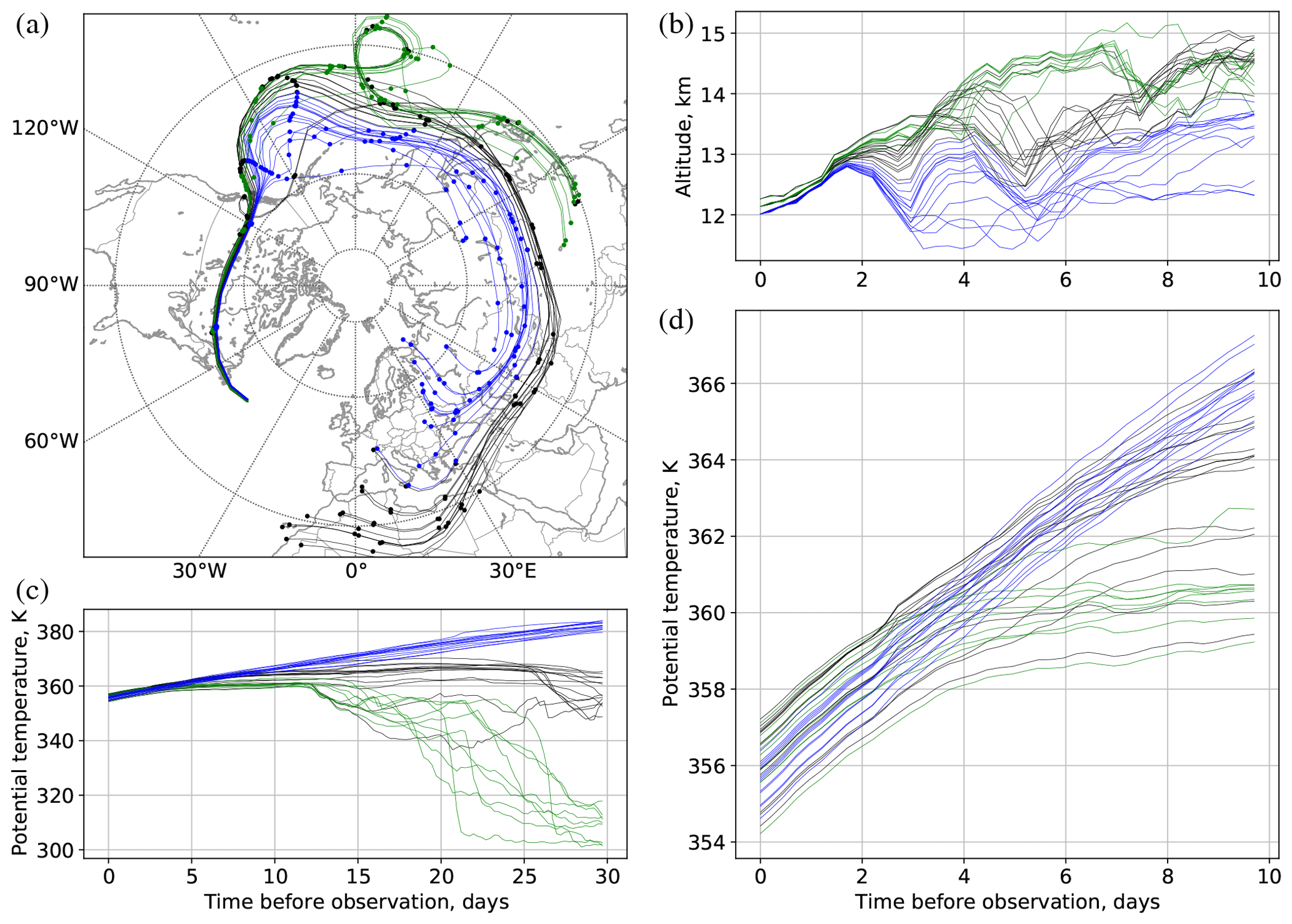
Figure 9 The backward trajectories for some of the air parcels found within 50 km from 48.5^∘ N, 43.5^∘ W, at altitudes between 12 and 12.4 km. We distinguish between groups of air parcels that have descended (blue), ascended (green) and remained at similar potential temperature levels (black) over the last 30 d before observation on 7 October. Panel (a) shows horizontal trajectories with circular markers every 24 h, (b) altitude and (c, d) potential temperature.

To demonstrate the effect of an RWB event more explicitly, Fig. 9 shows the very different trajectories of some of the air parcels observed in a small cylindrical volume 100 km in diameter and 400 m high shown as a green rectangle in Fig. 7e. Trajectories of three groups of air parcels coming from very different potential temperature levels are shown. The RWB event around 3 d before observation can be seen both as a slight disturbance in potential temperature and as trajectories from very different locations coming together around that time to form an air mass that was eventually observed by GLORIA. Although the potential temperature changes due to RWB are small, these events cause significant changes in altitude that, in a high-wind-shear environment around the polar jet, dramatically alter air parcel trajectories and long-term potential temperature trends.

Figure 10 gives further insight into the vertical transport of observed air parcels, the origin of these parcels and troposphere-to-stratosphere transport (TST) pathways. Figure 10a shows the temperature of tropopause crossing. Figure 10b shows the origin of air parcels in terms of potential temperature change. We can distinguish between the two old air filaments that have descended from the stratosphere (black circles) that match the retrieved old air structures, the air in between and to the southeast of the filaments that has been isentropically transported into the stratosphere and has less stratospheric tracers, and the turbulent troposphere below ≈9.5 km with low ozone and nitric acid values. The young air filament just above the upper filament marked in circles has been displaced during a Rossby wave breaking event. Its signature can be seen in Fig. 7a between the upper old air filament marked with white circles and a small old air blob at 43.5^∘ W, around 13 km altitude. Figure 10c shows the distribution of potential temperatures at which the observed air parcels entered the stratosphere (maximum potential vorticity gradient tropopause was used to determine the entry point) and the origin of these parcels¹. It demonstrates two distinct TST pathways. The first pathway is direct isentropic transport from the TTL to the extratropical stratosphere. The air travelling via this pathway enters the stratosphere at high potential temperature values, corresponding to a peak in Fig. 10c above 355 K. This pathway plays a major role, as expected for this region (Holton et al., 1995; Pan et al., 2009). The second pathway is via the lower potential temperature levels and corresponds to the second peak in the same figure between 330 and 350 K. Both air from TTL and air vertically uplifted from extratropical troposphere enters via this pathway. Our observations show that this potential temperature range does indeed contain the most strongly mixed air (see Fig. 4). Although a significant fraction of air entering the stratosphere had been in the PBL within the last 60 d (dotted red line in Fig. 10c), only a small part of it has not travelled through the TTL since then (dotted blue line in the same figure). This explains low water vapour VMRs in the region of the hexagonal flight pattern (Fig. 2, 16:15 to 17:42 UTC). Finally, Fig. 10d shows where the air that has entered the stratosphere has experienced strongest uplift. One can clearly see that the uplift in the tropics dominates; TST from extratropical upper troposphere involves a lot of air uplifted in the tropics and, in some cases, mixed with extratropical air masses.

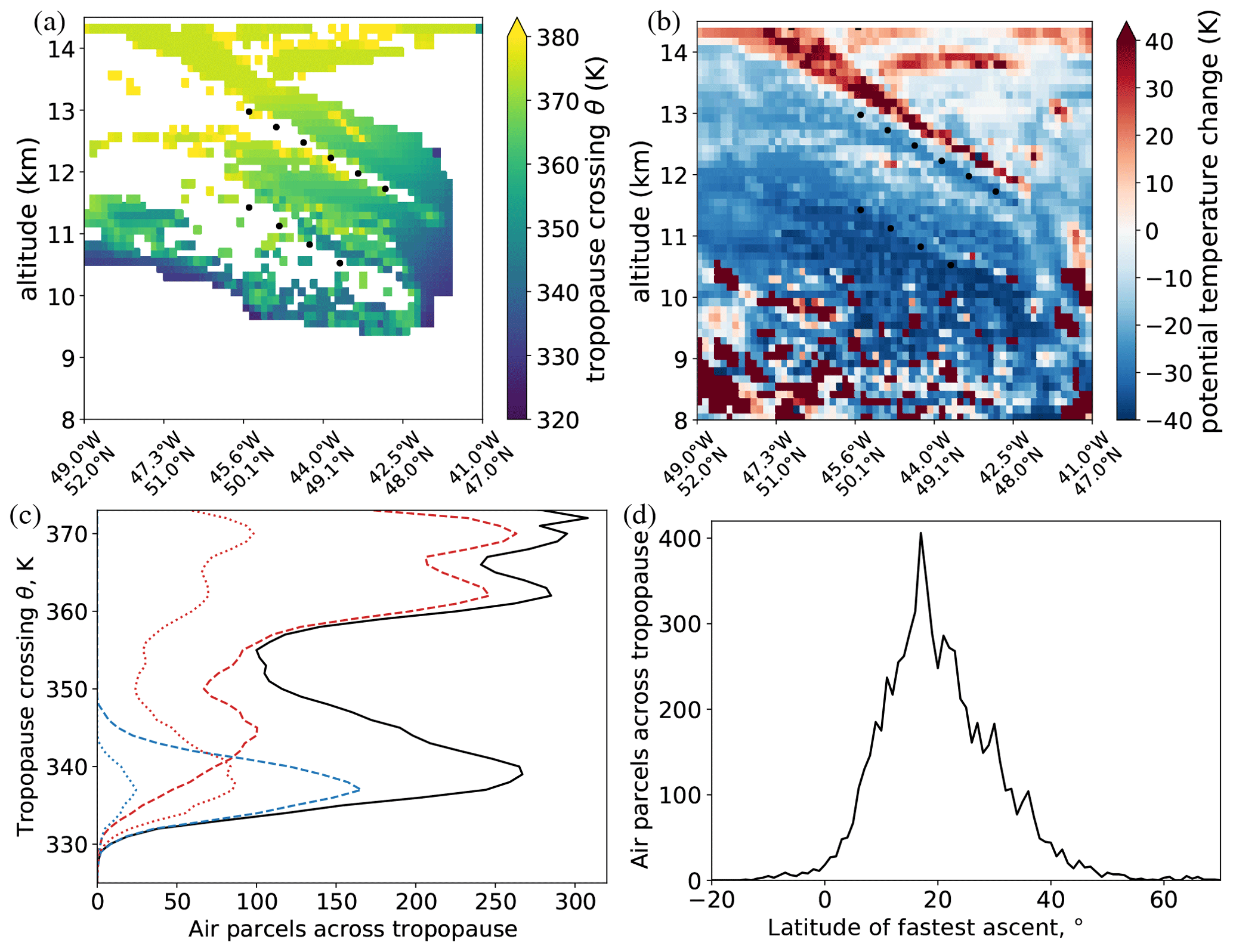
Figure 10 Panel (a) shows the potential temperature of tropopause crossing for the parcels that crossed tropopause within the last month. Panel (b) shows the change in potential temperature of observed air parcels within the last month. Black circles in panels (a) and (b) mark retrieved old air filaments; they are at the same positions as the white circles in Fig. 7. Panel (c) shows the distribution of potential temperature of tropopause crossing for the observed air parcels (black line). Other lines show how many of these parcels have been to TTL within last 30 d (dashed red line), extratropics below 330 K potential temperature within the last 30 d (dashed blue line), PBL within the last 60 d (dotted red line) and PBL within the last 60 d but not TTL (dotted blue line). All lines show the 5 K running mean. Panel (d) shows the latitude of fastest ascent (over 1 d) in potential temperature for the parcels shown in panel (c).

3.3 Origins of nitric acid enhancement above the tropopause

Nitric acid (HNO₃) is produced in the stratosphere (mainly from NO_x) and removed in the troposphere by washout. Hence, tropospheric HNO₃ mixing ratios can be as low as 0.1 ppbv or less. Due to the similarity of their source and sink regions, HNO₃ and O₃ typically display a very compact relationship within the stratosphere. Popp et al. (2009) give a simple linear relation between the two gases, which typically holds within 15 % in the stratosphere for ozone concentrations higher that 150 ppbv:

$$\begin{array}{}\text{(1)}& {\mathrm{HNO}}_{\mathrm{3}}=(\mathrm{0.00256}\pm \mathrm{0.000154}){\mathrm{O}}_{\mathrm{3}}-(\mathrm{0.0922}\pm \mathrm{0.0886})\mathrm{ppbv}.\end{array}$$

The tracer–tracer correlation of ozone and nitric acid for the 3-D tomographic retrieval is shown in Fig. 11. We can distinguish between several types of air masses in this tracer–tracer space. There is a HNO₃-poor tropospheric branch (HNO₃ < 0.2 ppbv), which consists solely of air parcels located below the dynamical tropopause (around 330 K here). A “deep stratospheric” branch conforms to the relationship of Eq. (1) within the prescribed ±15 % tolerance and consists mainly of air parcels above 360 K potential temperature. Air along the flight path falls into this category based on both GLORIA and in situ measurement data. Most of observed stratospheric air parcels have slightly enhanced HNO₃ values (between +15 % and +50 % HNO₃ compared to Eq. 1). Finally, there is the air mass with strongly enhanced HNO₃ values around the tropopause, clearly seen in Fig. 7. It has >1.25 ppbv HNO₃ and potential temperature of 330–350 K. Evidence of mixing between this air mass and its surroundings can be seen as linear structures in Fig. 11.

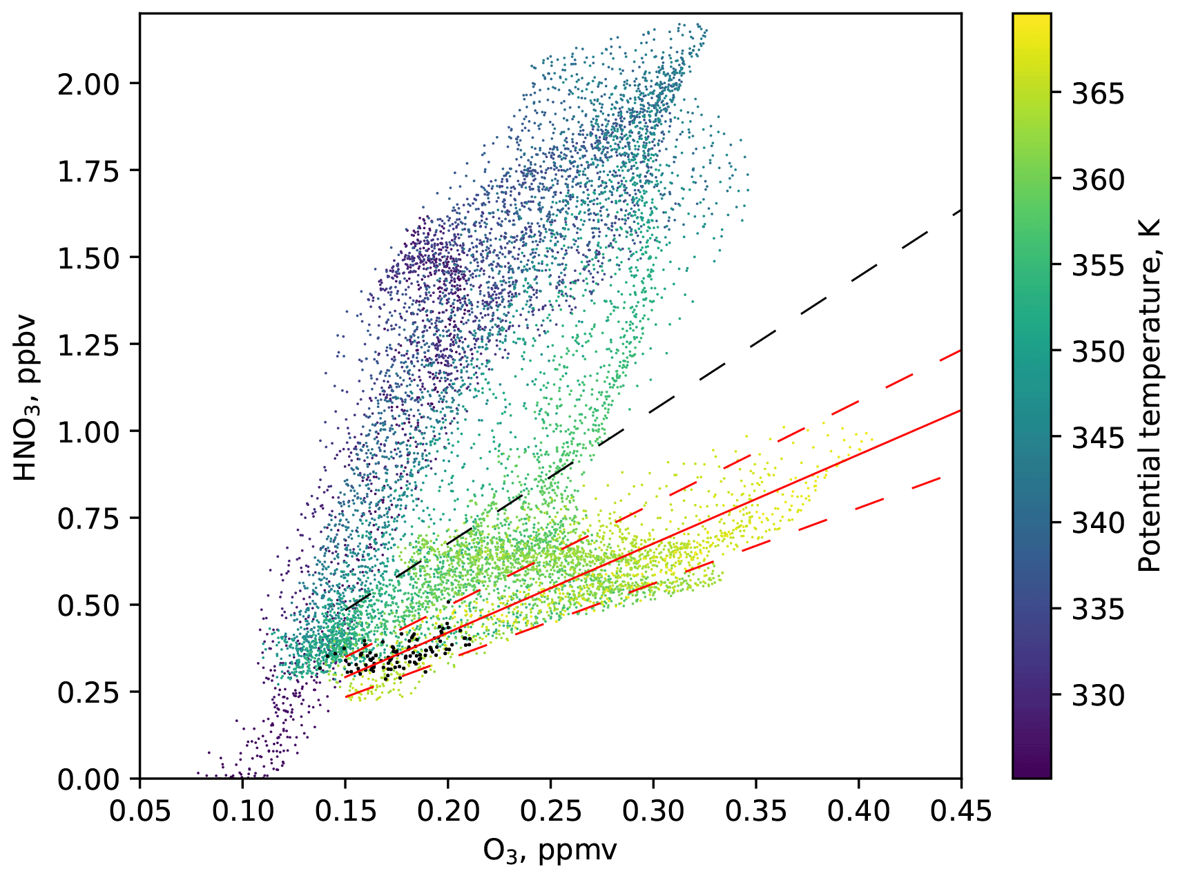
Figure 11 Ozone–nitric acid tracer–tracer correlation. Solid red line represents linear relationship of ozone and nitric acid typical for the stratosphere. Dashed red lines indicate the ±15 % HNO₃ compared to that relationship; dashed black line indicates +50 % HNO₃. Black dots represent in situ measurement data (see Appendix C for details); dots of the shown colour scale represent GLORIA data. Maximum potential vorticity gradient tropopause was used here.

It is clear from the argument above that the strong HNO₃ enhancement seen in Fig. 7b–c at the altitude of around 11.5 km could not be a consequence of STE alone. The most important tropospheric source of HNO₃ is conversion from NO_x, which, in turn, is produced mostly by fossil fuel burning (24 Tg N yr⁻¹), biomass burning (8 Tg N yr⁻¹), soil emissions (12 Tg N yr⁻¹) and lightning ((9 Tg N yr⁻¹)) (Price et al., 1997; Nesbitt et al., 2000). All of these sources, except for lightning, release NO_x into the boundary layer, where its lifetime is often below 1 d (Tie et al., 2001), and any HNO₃ produced is subject to washout. Therefore, despite lower total emissions, lightning is the most important source of NO_x in the upper troposphere (Zhang et al., 2000, 2003).

Backward trajectories were used to investigate whether the air masses with enhanced HNO₃ values could have been influenced by lightning. The air parcels observed on 7 October only came into proximity of significant lightning activity around 8 d before the measurement. That was also the time when the structures around the enhanced HNO₃ air masses were formed; i.e. it is the earliest time when the measured air parcels constituted a relatively compact group (Fig. 8). Figure 12 shows the positions of the air parcels with more than 2 ppbv HNO₃ and other air parcels observed by GLORIA on 29 September and the map of lightning activity that day. We see that some of the observed air parcels came into close proximity to the lightning strikes over France, Germany, Belgium and the Netherlands. They are both located below 5 PVU (close to the tropopause) and close by horizontally: the separation of the order of 100 km is small considering that these air masses were traced back almost all the way around the pole over 8 d. A large proportion of these air parcels are HNO₃ rich, and conversely, a significant proportion of HNO₃-rich air is located close to the lightning activity. Also, the time of 8 d between NO_x emission and HNO₃ measurement would have been sufficient for NO_x to HNO₃ conversion based on, e.g. Jaeglé et al. (1998). It is therefore possible that the highest HNO₃ values observed on 7 October were due to lightning. The lightning positions were obtained from very-low-frequency (VLF) radio observations (https://lightningmaps.org, last access: 10 November 2020; Narita et al., 2018).

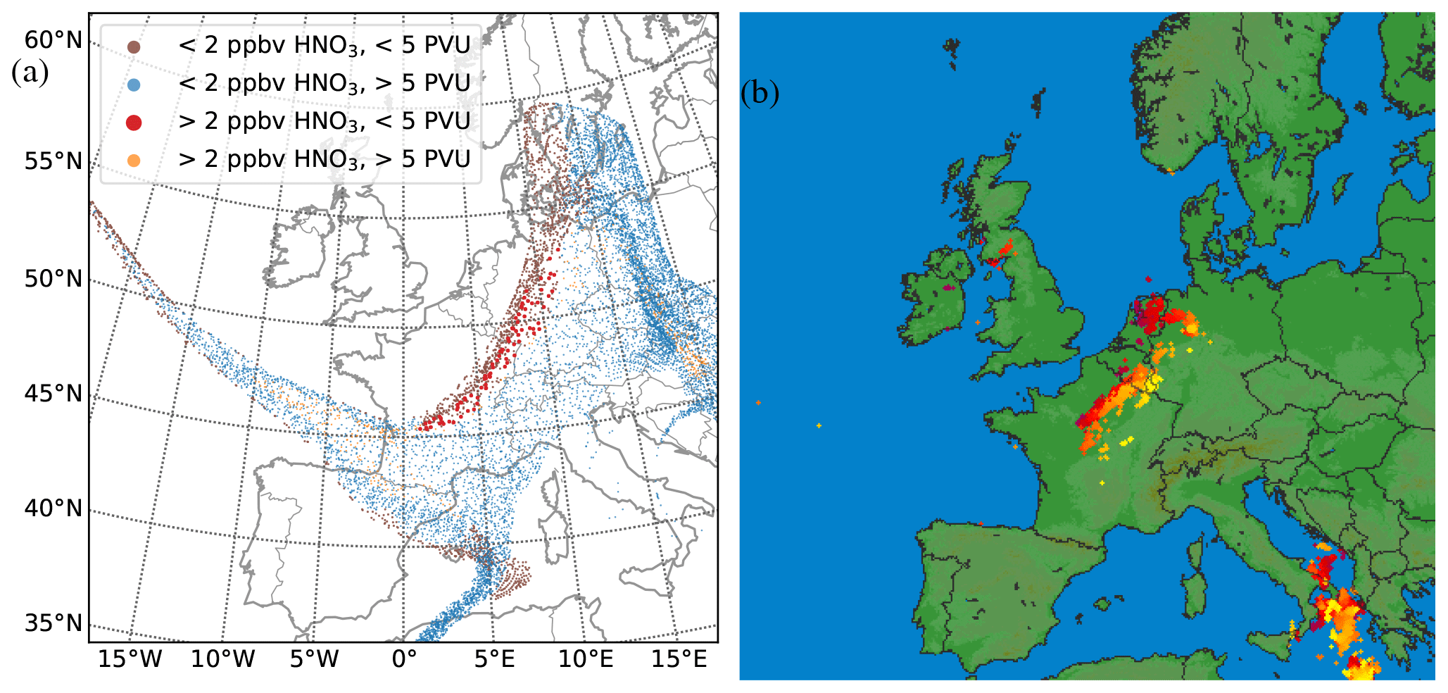
Figure 12 Panel (a) shows the positions of air parcels observed as part of the 7 October 3-D retrieval on 29 September 18:00 UTC (8 d before measurement). Air parcel colouring: brown – less than 2 ppbv HNO₃, less than 5 PVU; light blue – less than 2 ppbv HNO₃, more than 5 PVU; red (larger markers) – more than 2 ppbv HNO₃, less than 5 PVU; orange – more than 2 ppbv HNO₃, more than 5 PVU. HNO₃ VMRs considered are from the 7 October 3-D retrieval. Panel (b) shows lightning strikes between 29 September 18:00 UTC and 30 September 00:00 UTC in the area, based on very-low-frequency (VLF) radio observations. Lightning strikes are indicated by purple-to-yellow colour scale, depending on their time of occurrence within the given period.

3.4 The thin filament of the 9 October flight

The breaking Rossby wave event seen on 7 October was observed again during a flight on 9 October. No measurements suitable for tomography were taken during this flight, and the 2-D data for O₃, HNO₃ and H₂O are shown in Fig. 13. ECMWF forecasts before the flight led us to expect that the breaking wave would be stretched into a thin filament, shown as the 2 PVU contour in Fig. 1b extending from 70^∘ N, 0^∘ E, to 51^∘ N, 12^∘ E (dashed black line). The filament was crossed twice in both directions and can indeed be seen as old air structures around 11:00 and 14:00 UTC. The old air (ozone- and nitric-acid-rich) parts of the filament are very thin (some are only around 35 km across). The air mass that filled the hexagon (400 km in diameter) on 7 October was also stretched into a filament of 30 km thickness in its narrowest parts. Using backward trajectories, the air parcels that were measured both as part of the tomographic 3-D retrieval on 7 October and 2-D retrieval on 9 October were identified. They are highlighted by horizontal green hatches in Fig. 13.

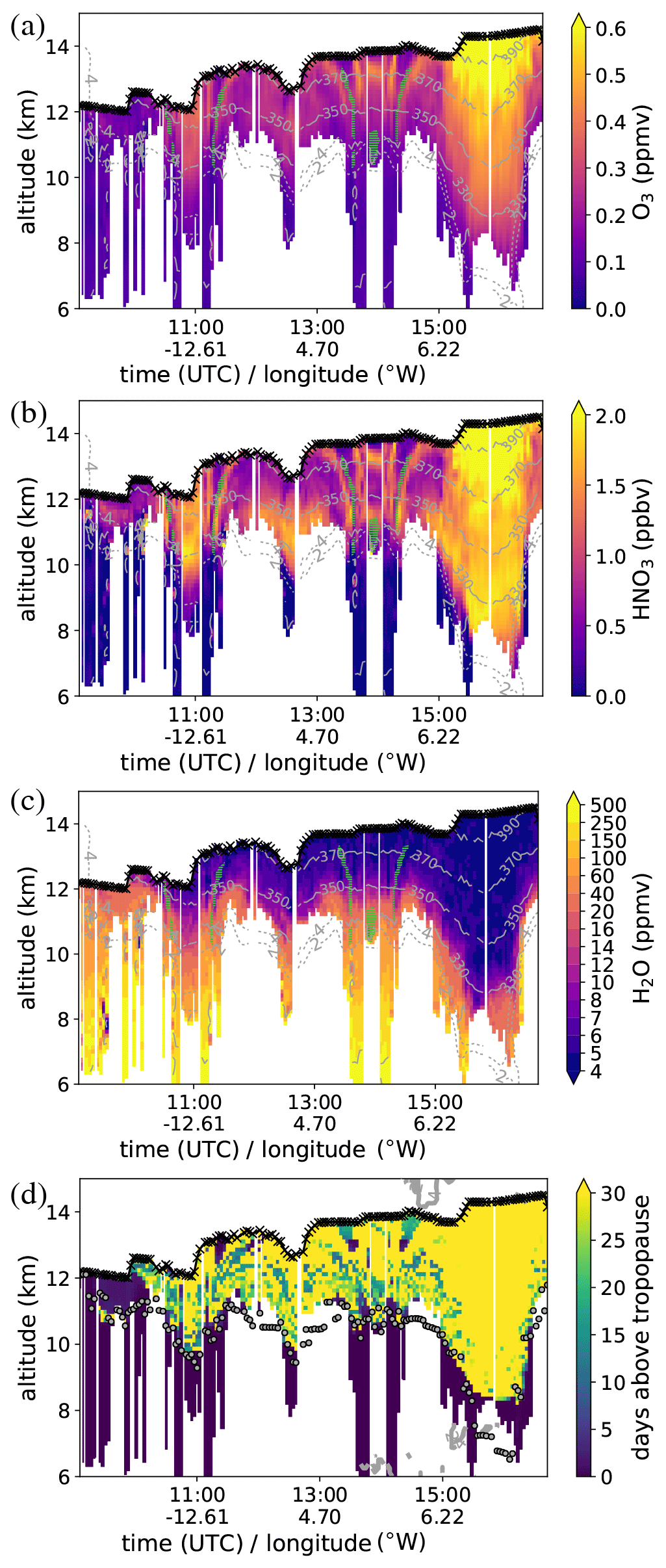
Figure 13 2-D data from the 9 October flight. Ozone (a), nitric acid (b) and water vapour (c) retrievals with stratosphere residence time plot (d) for the same air parcels. Isentropes are shown as thin solid lines; 2 and 4 PVU contours are shown as thick dashed lines. Green hatches represent air parcels observed by GLORIA on 7 October.

As before, a plot showing the stratosphere residence time is provided in Fig. 13d. Note the qualitatively different nature of younger air structures compared to previous plots of this sort and lack of filamentation in this region, generally less affected by planetary waves. The only young air structures that significantly exceed the instrument resolution are found around the filament originating from a breaking Rossby wave. A O₃–HNO₃ tracer–tracer plot for the air parcels observed in both flights is shown in Fig. 14. The general positive correlation between O₃ and HNO₃ and the enhanced HNO₃ values remain in the retrieval of 9 October. Slightly more parcels show tropospheric ozone and nitric acid values; these could be strongly diluted by tropospheric air or a result of collocation inaccuracies. The maximum concentrations of both tracers are now slightly lower, and there are more air samples with tracer concentrations closer to the mean values for the filament (e.g. more air parcels around 0.17 ppmv of ozone and 0.65 ppbv of nitric acid), while the distinct outlying branches, such as the highest HNO₃ enhancement and the purely stratospheric branch (around solid red line), are noticeably subdued. The latter branch also appears to be shifted towards the middling values of both tracers and is closer to the black line in Fig. 14. This is evidence of mixing, as tracer concentrations in all samples approach their average values. It is remarkable, however, that such a thin filament preserved the general tracer–tracer structure of an air mass of completely different shape, and that relatively little tropospheric influence is seen.

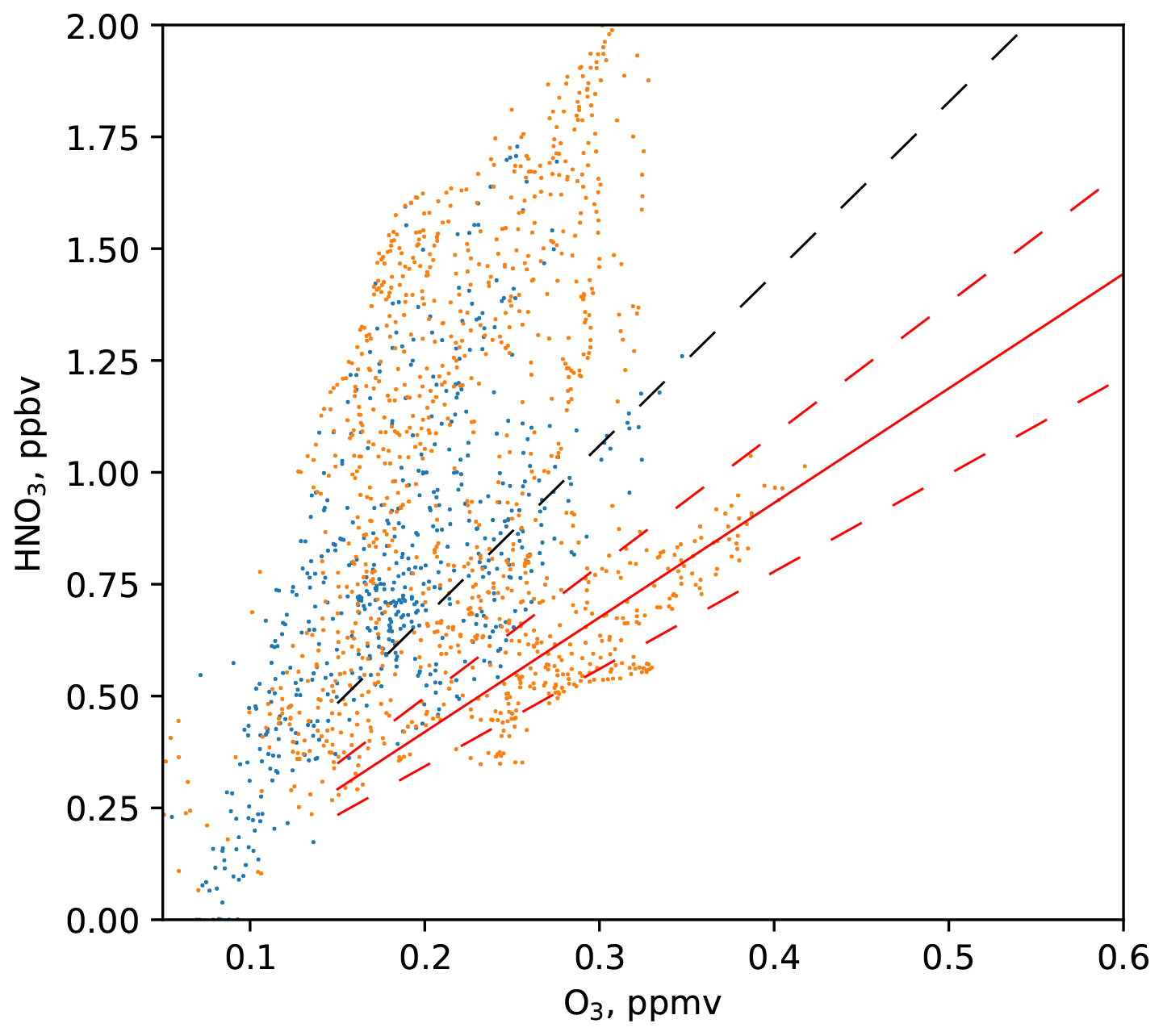
Figure 14 Ozone–nitric acid tracer–tracer correlation for air parcels observed in both flights. Tracer concentrations measured on 7 October (3-D tomographic retrieval) are shown in orange; those measured on 9 October are in blue. The solid red line represents linear relationship of ozone and nitric acid typical for the stratosphere. Dashed red lines indicate the ±15 % HNO₃ compared to that relationship; the dashed black line indicates +50 % HNO₃.

To further investigate the evolution of the air parcels observed on both flights, we determined the HNO₃ values in the hexagon based on the 9 October retrieval performed 2 d later. Air parcels from the 9 October 2-D data product were traced back to the hexagon. Each grid point inside the hexagon was assigned the HNO₃ volume mixing ratio of the closest back-traced parcel. If no parcel was traced back to a particular point within 100 km horizontally or 0.4 km vertically, the HNO₃ volume mixing ratio was deemed undetermined. One vertical cut through the HNO₃ reconstruction obtained in this manner is shown in Fig. 15, with a cut through the actual 3-D retrieval from 7 October shown for comparison. We can see that the tracer structure obtained by back tracing reflects many of the features in the tomographic retrieval, just with a lot lower resolution, since the 3-D retrieval grid has far more points than the number of air parcels that could be traced back to the 3-D retrieval volume from the observations 2 d later. The contrast (i.e. the difference between the highest and lowest HNO₃ VMRs) is lower for the back-traced data, suggesting that some mixing took place between the flights. This comparison demonstrates, however, that the thin filament, although clearly irreversibly separated from air masses around the polar jet, is still not fully mixed and “remembers” its past.

Figure 15 (a) HNO₃ volume mixing ratios on a vertical cut inside the hexagonal flight pattern based on back-traced 9 October measurements. (b) HNO₃ volume mixing ratios from the 7 October tomographic 3-D retrieval on the same vertical cut for comparison.

4 Conclusions

The UTLS in the Rossby wave surf zone is a highly interesting region of the atmosphere characterised by sharp gradients and fine structure of the tracer distributions that are very challenging to observe directly. Mixing in the Rossby wave surf zone has a major role on stratosphere–troposphere exchange (STE). Previous studies have shown that cross-tropopause transport into the extratropical lower stratosphere occurs mainly above the Atlantic and Pacific oceans and is most likely driven by Rossby wave breaking events (e.g. Kunz et al., 2015; Vogel et al., 2016). A Rossby wave breaking event was observed with the GLORIA instrument during two research flights 2 d apart. Both standard 2-D data sets and 3-D tomographic data of trace gas volume mixing ratios were acquired. Signs of enhanced mixing between stratospheric and tropospheric air parcels were seen near the polar jet with some transport of water vapour into the stratosphere. Mixing line analysis with the help of backward trajectories gave some indication on what the mixing timescales in this region could be. The observations performed in the first flight showed complex vertical structure in stratospheric tracers (ozone and nitric acid) with heavy filamentation, related to several Rossby wave breaking events 3 to 8 d before observation. With the help of CLaMS backward-trajectory calculations, much of the observed tracer structure can be understood as stirring and mixing of air masses of tropospheric and stratospheric origins. There are still unexpected aspects: for instance, the filaments were not only slanted in space but also stretched across different potential temperature levels. Therefore, even though these filaments were still sharply defined in the tracer structure and not strongly mixed, they could subsequently be erased by isentropic mixing. The backward-trajectory calculations revealed large amounts of air with histories indicative of horizontal transport from the lower-latitude troposphere and matching tracer signatures were found in the observations. Air masses from the extratropical troposphere were located mostly at the lowest altitudes of the observed part of the stratosphere. However, we found strongly uplifted (by more than 10 K) filaments, closely related to Rossby wave breaking events, and their histories were consistent with the measured tracer content. Just above the tropopause, nitric acid was enhanced by far more than could be explained by descent of air from the deep stratosphere. It is demonstrated in our study that NO_x production by lightning activity was a likely cause of this nitric acid enhancement. In the late stage of the RW breaking event, a filament containing air masses rich in stratospheric tracers became very long and thin (horizontal width was down to 30 km at some altitudes) and was advected away from the polar jet. Some of the air masses of the filament were observed during both flights (7 and 9 October) and showed a reduced contrast in tracer VMRs in the second flight indicating some mixing of the filament with its immediate surroundings, but the tracer structures seen during the first flight were still traceable in the data from the second. This direct observation of mixing provides a valuable data set for validation of mixing implementations in models.

A direct comparison of the full 3-D structure to model data in such detail would not have been possible with any other observational technique. Airborne observation of a significant number of air parcels twice with 2 d in between the measurements was also possible only due to the altitude range of GLORIA data and the unique 3-D capability of the instrument.

Appendix A: GLORIA retrieval technique

The GLORIA tomographic retrieval works by combining the JURASSIC2 fast radiative transfer model (Hoffmann et al., 2008; Ungermann et al., 2010) with an iterative inverse modelling scheme. The main idea of this scheme can be presented as follows. Let vector y represent a set of GLORIA radiance measurements and let vector x represent a discrete representation of the state of the atmosphere to be retrieved. In practice, x would contain assumed temperature and trace gas concentration values for each point in the retrieval grid. Using the forward model, one can calculate a vector F(x) – a simulation of the radiances GLORIA would measure if the atmosphere were indeed in the state x. Then the retrieval works by iteratively minimising the following quantity, which we call the cost function

$$\begin{array}{}\text{(A1)}& \begin{array}{rl}J\left(\mathit{x}\right)& ={\left(\mathit{F}\left(\mathit{x}\right)-\mathit{y}\right)}^T{\mathbf{S}}_{\mathit{ϵ}}^{-\mathrm{1}}\left(\mathit{F}\left(\mathit{x}\right)-\mathit{y}\right)+\\ & {\left(\mathit{x}-{\mathit{x}}_{\mathrm{a}}\right)}^T{\mathbf{S}}_{\mathrm{a}}^{-\mathrm{1}}\left(\mathit{x}-{\mathit{x}}_{\mathrm{a}}\right).\end{array}\end{array}$$

The first term in the sum measures how strongly the simulated measurements F(x), i.e. what GLORIA would measure if atmosphere state were x, differs from the actual measurement y. The covariance matrix ${\mathbf{S}}_{\mathit{ϵ}}^{-\mathrm{1}}$ contains information about the instrument accuracy. Large values of this term would mean that state x is unlikely, as it does not agree with the measurements.

The second term in the sum measures how well x fits our general knowledge of the atmosphere. Here, x_a is the a priori atmospheric state. A climatology, or low-resolution model data, can be used for this purpose. An atmospheric state that deviates very strongly from the a priori state is considered unlikely. The covariance matrix ${\mathbf{S}}_{\mathrm{a}}^{-\mathrm{1}}$ is typically non-diagonal; its purpose is not only to rule out atmospheric states that differ from the a priori state but also to suppress states that are discontinuous, have sharp jumps in atmospheric quantities or are otherwise unphysical. We construct this matrix to represent the exponential covariance. For two points in the atmosphere with the Cartesian coordinates $(x,y,z)$ and $(x^{\prime },y^{\prime },z^{\prime })$, respectively (z-coordinate vertical), the exponential covariance between the values of an atmospheric quantity at these points is

$$\begin{array}{}\text{(A2)}& \begin{array}{rl}& C\left((x,y,z),(x^{\prime },y^{\prime },z^{\prime })\right)=\\ & {\mathit{\sigma }}^{\mathrm{2}}\exp \left[-\sqrt{{\displaystyle \frac{{\left(x-x^{\prime }\right)}^{\mathrm{2}}}{L_{\mathrm{h}}^{\mathrm{2}}}}+{\displaystyle \frac{{\left(y-y^{\prime }\right)}^{\mathrm{2}}}{L_{\mathrm{h}}^{\mathrm{2}}}}+{\displaystyle \frac{{\left(z-z^{\prime }\right)}^{\mathrm{2}}}{L_{\mathrm{v}}^{\mathrm{2}}}}}\right].\end{array}\end{array}$$

Hence, σ describes the magnitude the expected departure from the a priori values for an atmospheric quantity, and L_h, L_v determine the typical length scales of structures in horizontal and vertical directions, respectively. The relevant parameters for the retrieval in this paper are given in Table A1.

Table A1 Regularisation parameters for 3-D retrieval.

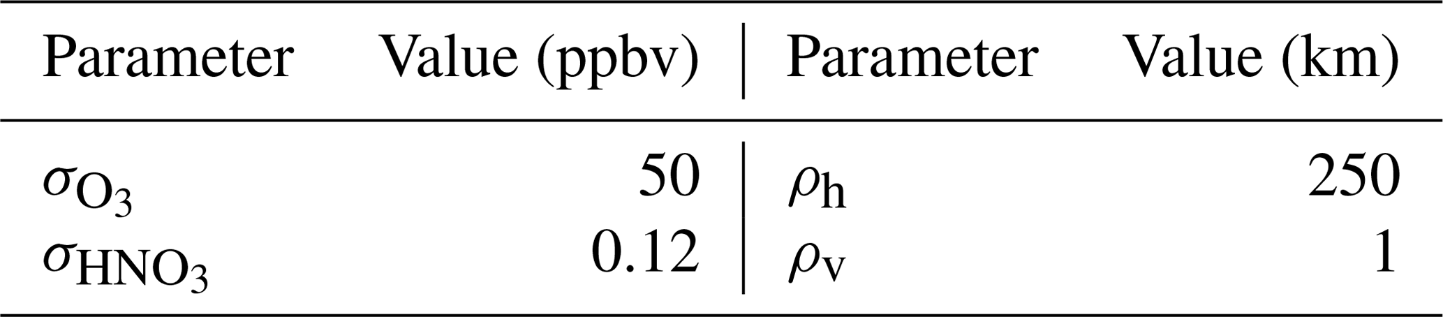
The standard deviations ${\mathit{\sigma }}_{{\mathrm{O}}_{\mathrm{3}}}$ and ${\mathit{\sigma }}_{{\mathrm{HNO}}_{\mathrm{3}}}$ were obtained by computing the standard deviation of in situ data for each tracer (shown in Appendix C for result validation). The ratio of horizontal and vertical correlation lengths ρ_h / ρ_v was set to 250, as this was estimated to be a typical aspect ratio for lower stratosphere (Haynes and Anglade, 1997) and also seems to match the aspect ratios of structures that form in CLaMS backward-trajectory runs (Sect. 3.2). The final values of ρ_h and ρ_v were then selected to optimise the resolution of the retrieval.

Appendix B: Tomographic retrieval error estimation

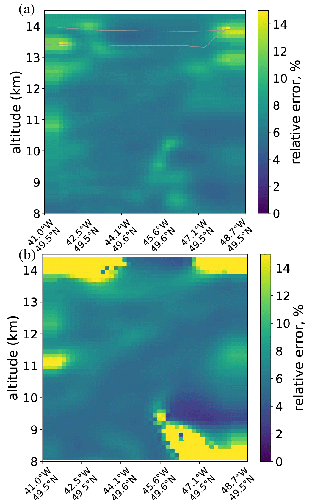
The data quality and expected errors of tomographic retrieval differ depending on the position of the point where these errors are calculated with respect to the flight path (hexagonal part of pattern). The relative errors for HNO₃ and O₃ were estimated for each point on the retrieval grid using a Monte Carlo based technique (Ungermann, 2013; Krasauskas et al., 2019). The particular error estimate calculated here includes measurement error and error due to inaccuracies of the retrieval method but does not include errors due to imprecise knowledge of atmospheric parameters (pressure, CO₂ concentration, etc.) that are required for retrieval and taken from external sources, mostly models.

Results of the calculation are presented as a vertical cut through the retrieved 3-D volume (Fig. B1). The same cut as in Fig. 7 (left) was used. One can confirm that, as expected, the data quality is best under the centre of the hexagonal flight pattern and quickly gets worse just outside the hexagon. Ozone retrieval around the flight path itself also seems problematic and should be interpreted with care. The average error values for measurements at 11 to 12 km altitude with horizontal distance of up to 200 km from the centre of the hexagonal flight pattern are given in Table B1. The table also contains estimates for linear retrievals at the same altitude range. They were estimated from the instrument noise and retrieval method uncertainties in a linear manner described in Ungermann et al. (2012).

Figure B1 3-D tomography relative error, Monte Carlo estimate: (a) ozone; (b) nitric acid.

Table B1 Average measurement error for 11 to 12 km altitude.

Appendix C: Tomographic retrieval validation using in situ instrument data

To validate the 3-D data products, we have performed a comparison with in situ measurements. During WISE ozone volume mixing ratio were measured by the Fast Airborne Ozone instrument (FAIRO; Zahn et al., 2012). The Atmospheric Nitrogen Oxides Measuring System (AENEAS; Ziereis et al., 2004) was also on board and provided NO_y and NO data products. In the UTLS, one can generally identify the total reactive nitrogen as the sum of volume mixing ratios of the following gases (ignoring the ones with typically much lower VMRs):

$$\begin{array}{}\text{(C1)}& {\mathrm{NO}}_y\approx \mathrm{NO}+{\mathrm{NO}}_{\mathrm{2}}+{\mathrm{HNO}}_{\mathrm{3}}+\mathrm{PAN}+{\mathrm{ClONO}}_{\mathrm{2}}.\end{array}$$

The volume mixing rations of NO₂, PAN and ClONO₂ are all typically at least 1 order of magnitude lower than that of HNO₃ considering the latitude and season of observation. PAN and ClONO₂ can be obtained from GLORIA data, and NO₂ is a relatively well-mixed tracer which we estimated based on WACCM model data. HNO₃ can hence be derived from AENEAS data for GLORIA validation purposes.

The comparison of GLORIA data and the in situ instruments is presented in Fig. C1. There are two important considerations that have a significant effect on the quality of a match to in situ data that can expected. Firstly, GLORIA measures trace gas concentrations along its line of sight, with a vertical resolution of about 200 m and horizontal resolution of 20 km. Since the whole line of sight (for usable measurements) is actually below the flight altitude, the highest-altitude data available cannot be regarded as measured from the aircraft location but rather from the location centred around ≈100 m below the aircraft and ≈10 km to the side of it. The result is imperfect spatial coincidence between GLORIA and in situ data, which can introduce biases into the comparison in the areas of high tracer gradients. Secondly, the GLORIA data product is valid for 16:50 UTC, while the in situ data are valid for the measurement time (see advection compensation description in Sect. 2.1). The data in Fig. C1 are corrected for this discrepancy in the sense that GLORIA data are provided for the actual air masses that the aircraft was flying through and not for the locations with respect to ground that were sampled. By 16:50 UTC, however, many of these air masses, especially the ones from the beginning of the flight, were advected outside of the best-resolved area of the hexagonal flight path (i.e. there were few overlapping measurements of these air parcels). This has a negative effect on data quality there. The errors for air further below flight altitude and closer to the centre of the hexagon should therefore be more accurate.

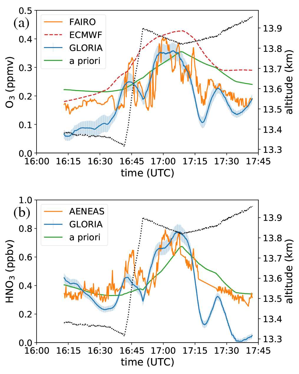
Figure C1 Comparison to in situ instrument data along the flight path. A priori data are from the WACCM model. Refer to the main text regarding details on in situ instruments and data.

Appendix D: Additional synoptic maps

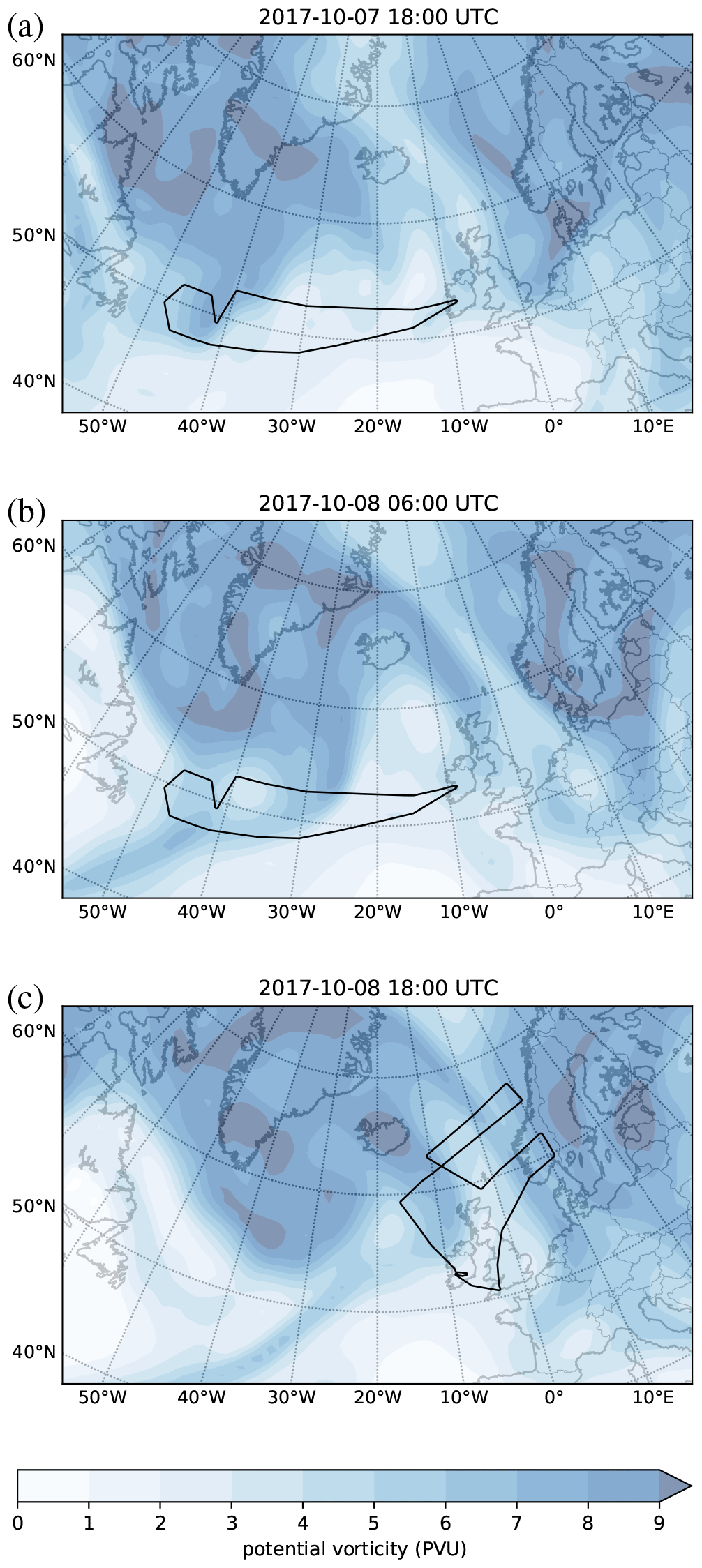
Figure D1 Potential vorticity at 340 K potential temperature level, 7–8 October. Black lines show flight paths.

Figure D2 Potential vorticity at 340 K potential temperature level, 9 October. Black lines show flight paths.