Role of oceanic ozone deposition in explaining temporal variability in surface ozone at High Arctic sites

Dry deposition is an important removal mechanism for tropospheric ozone (O₃). Currently, O₃ deposition to oceans in atmospheric chemistry and transport models (ACTMs) is generally represented using constant surface uptake resistances. This occurs despite the role of solubility, waterside turbulence and O₃ reacting with ocean water reactants such as iodide resulting in substantial spatiotemporal variability in O₃ deposition and concentrations in marine boundary layers. We hypothesize that O₃ deposition to the Arctic Ocean, having a relatively low reactivity, is overestimated in current models with consequences for the tropospheric concentrations, lifetime and long-range transport of O₃. We investigate the impact of the representation of oceanic O₃ deposition to the simulated magnitude and spatiotemporal variability in Arctic surface O₃.

We have integrated the Coupled Ocean-Atmosphere Response Experiment Gas transfer algorithm (COAREG) into the mesoscale meteorology and atmospheric chemistry model Polar-WRF-Chem (WRF) which introduces a dependence of O₃ deposition on physical and biogeochemical drivers of oceanic O₃ deposition. Also, we reduced the O₃ deposition to sea ice and snow. Here, we evaluate WRF and CAMS reanalysis data against hourly averaged surface O₃ observations at 25 sites (latitudes > 60^∘ N). This is the first time such a coupled modeling system has been evaluated against hourly observations at pan-Arctic sites to study the sensitivity of the magnitude and temporal variability in Arctic surface O₃ on the deposition scheme. We find that it is important to nudge WRF to the ECMWF ERA5 reanalysis data to ensure adequate meteorological conditions to evaluate surface O₃.

We show that the mechanistic representation of O₃ deposition over oceans and reduced snow/ice deposition improves simulated Arctic O₃ mixing ratios both in magnitude and temporal variability compared to the constant resistance approach. Using COAREG, O₃ deposition velocities are in the order of 0.01 cm s⁻¹ compared to ∼ 0.05 cm s⁻¹ in the constant resistance approach. The simulated monthly mean spatial variability in the mechanistic approach (0.01 to 0.018 cm s⁻¹) expresses the sensitivity to chemical enhancement with dissolved iodide, whereas the temporal variability (up to ±20 % around the mean) expresses mainly differences in waterside turbulent transport. The mean bias for six sites above 70^∘ N reduced from −3.8 to 0.3 ppb with the revision to ocean and snow/ice deposition. Our study confirms that O₃ deposition to high-latitude oceans and snow/ice is generally overestimated in ACTMs. We recommend that a mechanistic representation of oceanic O₃ deposition is preferred in ACTMs to improve the modeled Arctic surface O₃ concentrations in terms of magnitude and temporal variability.

1 Introduction

Tropospheric ozone (O₃) is the third most important greenhouse gas and a secondary air pollutant negatively affecting human health (Nuvolone et al., 2018) and plant growth (Ainsworth et al., 2012) due to its oxidative character. O₃ shows a large spatiotemporal variability due to its relatively short lifetime (3–4 weeks) in the free troposphere compared to other greenhouse gases. Its main sources are chemical production and entrainment from the stratosphere. Its main sinks are chemical destruction and deposition to the Earth's surface (Young et al., 2018; Tarasick et al., 2019). Understanding the Arctic O₃ budget is of particular interest because its remote location implies that anthropogenic sources and sinks are generally absent. This implies that these Arctic O₃ observations allow us to determine large-scale trends in tropospheric O₃ (Helmig et al., 2007b; Gaudel et al., 2020; Cooper et al., 2020). In the Arctic, routine tropospheric O₃ observations indicate an increasing trend up to the early 2000s which has been leveling off (Oltmans et al., 2013; Cooper et al., 2014) or decreasing at individual sites (Cooper et al., 2020) in the last decade. This upward trend can be attributed to increased emissions of precursors in the midlatitudes (Cooper et al., 2014; Lin et al., 2017), but stratosphere-to-troposphere transport may also have played a role (Pausata et al., 2012). Local emissions of precursors are expected to become an important source of Arctic O₃ concentrations due to the warming Arctic climate and increasing local economic activity (Marelle et al., 2016; Law et al., 2017). This underlines the need for understanding the sources and sinks of Arctic tropospheric O₃ and to accurately representing them in atmospheric chemistry and transport models (ACTMs).

On the global scale, dry deposition accounts for ∼ 25 % of the total sink term (Lelieveld and Dentener, 2000) in ACTM simulations and is especially important for the O₃ budget in the atmospheric boundary layer (ABL). Dry deposition in ACTMs is often represented as a resistance in series approach (Wesely, 1989). Herein, the total resistance r_t consists of three serial resistances: the aerodynamic resistance (r_a) representing turbulent transport to the surface, the quasi-laminar sublayer resistance (r_b) representing diffusion close to the surface and the surface resistance (r_s) expressing the efficiency of removal by the surface. The dry-deposition velocity (V_d) is then evaluated as the reciprocal of r_t. The r_a term mainly depends on the stability of the atmosphere and friction velocity (u_*) (Padro, 1996; Toyota et al., 2016). The r_b term also scales with u_* and varies with the diffusivity of the chemical species (Wesely and Hicks, 2000). Low-solubility gases like O₃ have a high r_s, in comparison to the relatively small r_a+r_b term, which dominates the magnitude of the O₃ dry-deposition velocity ($V_{\mathrm{d},{\mathrm{O}}_{\mathrm{3}}}$). Thus, accurately representing the surface uptake efficiency of O₃ is crucial. During episodes of low wind speeds, the r_a+r_b term can pose an additional restriction on the exchange of O₃ with oceans (Fairall et al., 2007).

Observed O₃ deposition to oceans (e.g., Chang et al., 2004; Clifford et al., 2008; Helmig et al., 2012) and coastal waters (e.g., Gallagher et al., 2001) is relatively slow (∼ 0.01–0.1 cm s⁻¹). However, oceanic O₃ is relevant for the global O₃ deposition budget due to the large surface area of water bodies (Ganzeveld et al., 2009; Hardacre et al., 2015). Recent experimental and modeling studies indicate the spatiotemporal variability in oceanic O₃ uptake efficiency (Ganzeveld et al., 2009; Helmig et al., 2012; Luhar et al., 2018). However, most ACTMs often use a constant O₃ surface uptake efficiency of 2000 cm s⁻¹ to water bodies, proposed by Wesely (1989), resulting in a simulated ocean $V_{\mathrm{d},{\mathrm{O}}_{\mathrm{3}}}$ of ∼ 0.05 cm s⁻¹. The observed $V_{\mathrm{d},{\mathrm{O}}_{\mathrm{3}}}$ shows a larger variability including also a dependency on wind speed and sea surface temperature (SST) (Helmig et al., 2012). The turbulence-driven enhancement by wind speed (Fairall et al., 2007) is complemented by a strong chemical enhancement of oceanic O₃ deposition associated with its chemical destruction through the oxidation of ocean water reactants such as dissolved iodide and dissolved organic matter (DOM) (Chang et al., 2004). Mechanistic O₃ deposition representations in models include the physical and biogeochemical drivers of the exchange of O₃ in surface waters (Fairall et al., 2007, 2011; Ganzeveld et al., 2009; Luhar et al., 2017, 2018). Dissolved iodide is deemed to be the main reactant of O₃ in surface waters (Chang et al., 2004) and therefore often applied in these representations. Some studies only consider dissolved iodide as a reactant (Luhar et al., 2017; Pound et al., 2020), whereas Ganzeveld et al. (2009) also included DOM as one reactant contributing to the chemical enhancement of oceanic O₃ deposition. These mechanistic deposition representations appeared to be crucial for O₃ dry-deposition modeling, the marine ABL O₃ concentrations and the potentially involved feedback mechanisms such as the release of halogen compounds as a function of O₃ deposition (Prados Roman et al., 2015).

Up until now, earlier studies on global-scale oceanic O₃ deposition (Ganzeveld et al., 2009; Luhar et al., 2017) evaluated monthly mean surface O₃ observations (Pound et al., 2020). The implementation of these mechanistic exchange methods in ACTMs, in particular the method proposed by Luhar et al. (2018) using a two-layer model representation (compared to a bulk layer version by Ganzeveld et al., 2009), results in a ∼ 50 % reduction in the global mean $V_{\mathrm{d},{\mathrm{O}}_{\mathrm{3}}}$ which affects the tropospheric O₃ burden (Pound et al., 2020). The mechanistic representation in Pound et al. (2020) especially results in a simulated decrease in $V_{\mathrm{d},{\mathrm{O}}_{\mathrm{3}}}$ to cold polar waters with relatively low reactivity. Simulated $V_{\mathrm{d},{\mathrm{O}}_{\mathrm{3}}}$ can be as low as 0.01 cm s⁻¹ compared to the commonly applied $V_{\mathrm{d},{\mathrm{O}}_{\mathrm{3}}}$ of 0.05 cm s⁻¹ in the constant surface uptake resistance approach (Pound et al., 2020). However, the hypothesized deposition reduction to cold waters is expected to substantially affect Arctic ABL O₃ concentrations on relatively short timescales (sub-monthly) and potentially improve operational Arctic O₃ forecasts, e.g., the air quality forecasts by the Copernicus Atmosphere Monitoring Service (CAMS) (Inness et al., 2019).

The evaluation of simulated oceanic O₃ deposition in the Arctic is hampered by a lack of O₃ ocean–atmosphere flux observations and consequently relies on a comparison of simulated and observed surface O₃ concentrations not only regarding the magnitude but in particular the temporal variability. We hypothesize that on synoptic timescales these concentrations are controlled by temporal variability in the main physical drivers of oceanic O₃ deposition, e.g., atmospheric and waterside turbulence mainly as a function of wind speed. Chemical enhancement of, e.g., iodide to O₃ deposition is anticipated to control the long-term (months) baseline level of $V_{\mathrm{d},{\mathrm{O}}_{\mathrm{3}}}$ more associated with anticipated long-term (e.g., seasonal) changes in ocean water biogeochemical conditions (Sherwen et al., 2019). This evaluation of Arctic spatiotemporal O₃ concentrations aims to better understand the role of ocean and sea ice deposition as a potentially important but also uncertain sink impacting Arctic air pollution (Arnold et al., 2016). Furthermore, the projected opening of the Arctic Ocean, as a result of climate change, urges us to improve our understanding of Arctic Ocean–atmosphere exchange.

We aim to identify and quantify the impact of a mechanistic representation of O₃ deposition in explaining observed hourly Arctic surface O₃ concentrations, both in terms of magnitude and temporal variability. A mesoscale coupled meteorology–atmospheric chemistry model is evaluated against a large dataset of pan-Arctic O₃ observations at a high-resolution (hourly) timescale for the end of summer 2008. Using a much higher spatial and temporal resolutions compared to other global modeling studies, we aim to evaluate to what extent the role of spatiotemporal variability in O₃ deposition explains observed surface O₃ concentrations particularly regarding temporal variability. We also indicate the role of meteorology in simulating these O₃ concentrations by nudging the simulated synoptic conditions towards an atmospheric reanalysis dataset.

2 Methods

2.1 Regional coupled meteorology–chemistry model

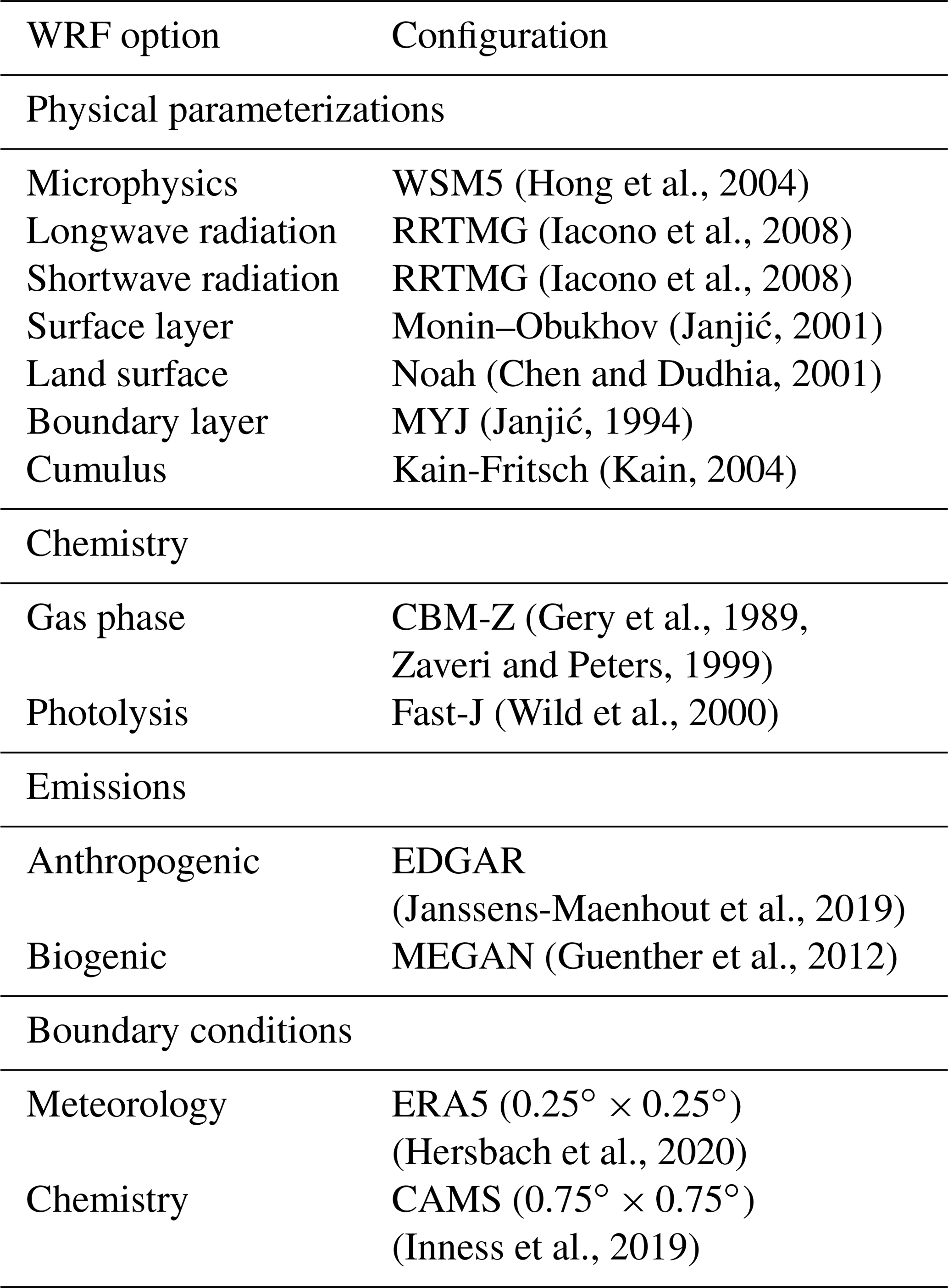
We use the Weather Research and Forecasting model (v4.1.1) coupled to chemistry (Chem) (Grell et al., 2005) and optimized for Polar regions (Hines and Bromwich, 2008). Polar-WRF-Chem (hereafter WRF) is a non-hydrostatic mesoscale numerical weather prediction and atmospheric chemistry model used for operational and research purposes. Figure 1 shows the selected study area including the locations of surface O₃ observational sites selected for this study (more information in Sect. 2.5). WRF is set up with a polar projection centered at 90^∘ N, 250 × 250 horizontal grid points (30 × 30 km resolution) and 44 vertical levels up to 100 hPa, with a finer vertical grid spacing in the ABL and lower troposphere. The simulation period is 8 August to 7 September 2008 including 3 d of spin-up. This end-of-summer 2008 period is chosen (1) to limit the role of active halogen chemistry during springtime (Pratt et al., 2013; Thompson et al., 2017; Yang et al., 2020) and (2) the additional availability of O₃ observations in the High Arctic over sea ice from the Arctic Summer Cloud Ocean Study (ASCOS) campaign (Paatero et al., 2009). The ECMWF ERA5 meteorology (0.25^∘ × 0.25^∘) (Hersbach et al., 2020) and CAMS reanalysis chemistry (0.75^∘ × 0.75^∘) (Inness et al., 2019) products are used for the initial and boundary conditions. Boundary conditions, SSTs and sea ice fractions are updated every 3 h to these reanalysis products to allow for the sea ice retreat during the simulation. Other relevant parameterization schemes and emission datasets have been listed in Table A1 and are mostly based on Bromwich et al. (2013).

Figure 1 WRF domain including sea ice and snow cover at the start of the simulation. Locations with surface observations O₃ are indicated in green (High Arctic), magenta (Remote) and cyan (Terrestrial) (see Sect. 2.5). The drifting path of the ASCOS campaign during the simulation is indicated with the black line.

2.2 Nudging to ECMWF ERA5

The first WRF simulation, without any adjustments to O₃ deposition, indicated that WRF was misrepresenting the temporal variability in surface O₃ observations, most prominently starting from a few days into the simulation. We hypothesize that this misrepresentation is caused by deviations in the synoptic conditions in the free-running WRF simulation. This was confirmed with a comparison of simulated and satellite observed wind speeds above oceans at a spatial resolution of 0.25^∘ × 0.25^∘ (Wentz and Meissner, 2004). To overcome the impact of this deficiency on our O₃ study, nudging is applied to ensure an optimal model evaluation with observations. Hence, WRF is nudged every 3 h to the ECMWF ERA5 specific humidity, temperature and wind fields in the free troposphere with nudging coefficients of 1 × 10⁻⁵, 3 × 10⁻⁴ and 3 × 10⁻⁴ s⁻¹, respectively.

2.3 Representation of ocean–atmosphere gas exchange

The Coupled Ocean-Atmosphere Response Experiment (COARE) (Fairall et al., 1996) has been developed to study physical exchange processes (sensible heat, latent heat and momentum) at the ocean–atmosphere interface. Later, COARE has been extended to include the exchange of gaseous species such as O₃, dimethyl sulfide (DMS) and carbon dioxide (CO₂) (Fairall et al., 2011). Many studies have used the COARE Gas transfer algorithm (COAREG) in combination with eddy-covariance measurements to study the effects of wind speed and sea state on ocean–atmosphere gas exchange (e.g., Helmig et al., 2012; Blomquist et al., 2017; Bell et al., 2017; Porter et al., 2020). Furthermore, the COAREG algorithm has also been previously used in global O₃ modeling studies (Ganzeveld et al., 2009). The choice for COAREG is further motivated by the consistent coupling with other species such as DMS.

Here we use COAREG version 3.6, which is extended with a two-layer scheme for surface resistance compared to the previous version described by Fairall et al. (2007, 2011). The two-layer scheme is similar to Luhar et al. (2018) building upon a first application of a one-layer version of COAREG by Ganzeveld et al. (2009). In that study, chemical enhancement of ocean O₃ deposition by its reaction with iodide was considered using a global climatology of ocean surface water concentrations of nitrate serving as a proxy for oceanic iodide concentrations (I${}_{\mathrm{aq}}^{-}$). Besides nitrate, satellite-derived chlorophyll-α concentrations have been used as a proxy for I${}_{\mathrm{aq}}^{-}$ (Oh et al., 2008). Since then, alternative parameterizations of oceanic I${}_{\mathrm{aq}}^{-}$ have been proposed (e.g., MacDonald et al., 2014) using SST as a proxy for this reactant. In COAREG, chemical reactivity of O₃ with I${}_{\mathrm{aq}}^{-}$ is present through the depth of the oceanic mixing layer. O₃ loss by waterside turbulent transfer is negligible in the top water layer (few micrometers), but is accounted for in the underlying water column. The waterside turbulent transfer term is especially relevant for relatively cold waters because the chemical enhancement term is then relatively low (Fairall et al., 2007; Ganzeveld et al., 2009; Luhar et al., 2017). The last two important waterside processes that determine the total O₃ deposition are molecular diffusion and solubility of O₃ in seawater which both depend on the SST. In Appendix B we list the formulation of the air side and waterside resistance terms in the COAREG routine applied in this study and show the sensitivity to the environmental factors wind speed, SST and I${}_{\mathrm{aq}}^{-}$ for typical Arctic conditions.

The COAREG algorithm is coupled such that WRF provides the meteorological and SST input for the COAREG routine. In turn, the COAREG calculated ocean–atmosphere exchange velocities are used in the WRF model to calculate the oceanic O₃ deposition flux replacing the default oceanic O₃ deposition fluxes calculated by the Wesely (1989) scheme reflecting use of the default constant r_s of 2000 s m⁻¹. For grid boxes with fractional sea ice cover, COAREG replaces the Wesely deposition scheme for the fraction that is ice free. Note that in this study, only O₃ ocean–atmosphere exchange is represented by COAREG not having modified simulations of ocean–atmosphere exchange of other compounds (e.g., DMS).

Moreover, we apply the monthly mean I${}_{\mathrm{aq}}^{-}$ distribution by Sherwen et al. (2019) (0.125^∘ × 0.125^∘ resolution) which applies a machine learning approach, namely the random forest regressor algorithm (Pedregosa et al., 2011), using various physical and chemical variables such as SST, nitrate, salinity and mixed layer depth. This distribution replaces the previously applied I${}_{\mathrm{aq}}^{-}$ estimations only using SST (Chance et al., 2014; MacDonald et al., 2014). At high latitudes, these I${}_{\mathrm{aq}}^{-}$ distributions are highly uncertain due to the limited number of observations. The choice for Sherwen et al. (2019) is motivated by the most accurate representation of observed I${}_{\mathrm{aq}}^{-}$ by the introduction of other predictors besides SST. Furthermore, this product will be further updated with newly available measurements. Figure C1 shows the spatial distribution of I${}_{\mathrm{aq}}^{-}$ used in the calculation of the O₃ deposition velocities. Using the Sherwen et al. (2019) distribution for August/September we found I${}_{\mathrm{aq}}^{-}$ concentrations ranging between 30 and 80 nM for the open oceans up to 130 nM in coastal waters. In MacDonald et al. (2014) and Chance et al. (2014), I${}_{\mathrm{aq}}^{-}$ is solely a function of SST which leads to I${}_{\mathrm{aq}}^{-}$ in the order of 5 to 50 nM and thus low reactivity and O₃ deposition velocities.

2.4 Deposition to snow and ice

Reported atmosphere–snow gas exchange spans a wide range of observed O₃ deposition velocities. Some studies even report episodes of negative deposition fluxes (emissions) over snow or sea ice (Zeller, 2000; Helmig et al., 2009; Muller et al., 2012). Clifton et al. (2020a) recently summarized observed O₃ deposition velocities to snow having a range of −3.6 to 1.8 cm s⁻¹ with most of the observations indicating a deposition velocity between 0 and 0.1 cm s⁻¹ for multiple snow-covered surfaces (e.g., grass, forest and sea ice). Generally, O₃ concentrations in the interstitial air of the snowpack are lower than in the air above making the snowpack not a direct source of O₃ in terms of emissions (Clifton et al., 2020a). However, the emissions of O₃ precursors from the snowpack can enhance O₃ production in the very stable atmosphere above the snowpack (Clifton et al., 2020a). Helmig et al. (2007a) investigated the sensitivity of a global chemistry and tracer transport model to the prescribed O₃ deposition velocity and found the best agreement between modeled and observed O₃ concentrations at four Arctic sites by applying deposition velocities in the order of 0.00–0.01 cm s⁻¹. Following Helmig et al. (2007a) we have increased the O₃ surface uptake resistance (r_s) for snow and ice land use classes to 10⁴ s m⁻¹. This corresponds to total deposition velocities of ≤ 0.01 cm s⁻¹, which is a reduction of ∼ 66 % compared to the Wesely deposition routine that is the default being applied in WRF (Grell et al., 2005).

2.5 Observational data of surface ozone

The new modeling setup, including nudging to ECMWF ERA5 and the revised O₃ deposition to snow, ice and oceans, is evaluated against observational data of pan-Arctic surface O₃ concentrations. We expect that the different representation of O₃ deposition mostly affects O₃ concentrations in the ABL. Therefore, we evaluate our simulations against hourly averaged surface O₃ observations from 25 measurement sites above 60^∘ N. These sites are further categorized in three site selections: “High Arctic”, “Terrestrial” and “Remote”. High Arctic refers to sites having latitudes > 70^∘ N and for which we expect that the deposition footprint is a combination of ocean and sea ice (e.g., Helmig et al., 2007b). The Terrestrial sites are located below 70^∘ N and show a clear diurnal cycle in observed O₃. Sites are characterized as Terrestrial when the average observed minimum nighttime mixing ratio is > 8 ppb smaller than the average observed maximum daytime mixing ratio during the ∼ 1 month of simulation. This criterion is based on a preparatory analysis of the observational data, footprint and site characteristics. The Remote sites have been identified as such based on their location below 70^∘ N and showing no clear diurnal cycle in O₃ concentrations. The analysis also includes the observations during the Arctic Summer Cloud Ocean Study (ASCOS) campaign, when the icebreaker Oden was located in the Arctic sea ice (Tjernström et al., 2012). In total, 25 surface O₃ measurement sites are included (Fig. 1), of which 6, 8 and 11 sites are characterized as High Arctic, Remote and Terrestrial sites, respectively. A full list of available measurement sites is available in Table D1.

2.6 Overview of performed simulations

In total, we perform two simulations. The first WRF simulation (NUDGED) is a run with the setup described in Sect. 2.1 and nudged with the synoptic conditions to the ECMWF ERA5 product as described in Sect. 2.2. The second simulation (COAREG) includes also includes the adjustments to the O₃ deposition to oceans as described in Sect. 2.3 and the O₃ deposition to snow and ice as described in Sect. 2.4. Furthermore, we also compare our results with the state-of-the-art CAMS global reanalysis data product (Inness et al., 2019). This product has a temporal resolution of 3 h, a spatial resolution of 0.75^∘ × 0.75^∘ and does not include a mechanistic representation of ocean–atmosphere O₃ exchange. CAMS assimilates satellite observations of O₃ but it does not assimilate O₃ observations from radiosondes or in situ measurement sites such as the 25 sites used in the evaluation presented here. This implies that lower-tropospheric O₃ is weakly constrained by observations in this CAMS product making an accurate model representation of the sources and sinks important. We opted to include the CAMS reanalysis data as another tool to study Arctic surface O₃ and to address potential limitations in its model setup. Moreover, CAMS is being widely used for air quality forecasts and assessments but also to constrain regional-scale modeling experiments such as presented in this study. Therefore, an analysis of the performance of the CAMS reanalysis data might also benefit future Arctic air quality assessments.

3 Results

3.1 Dry-deposition budgets and distribution

Figure 2a and b show the mean deposition velocities for the NUDGED and COAREG runs, respectively. As expected, in the NUDGED run (Fig. 2a) the mean $V_{\mathrm{d},{\mathrm{O}}_{\mathrm{3}}}$ to oceans is in the order of 0.05 cm s⁻¹. Furthermore, the spatial distribution shows a relatively low heterogeneity and no increase in deposition velocities towards the warmer waters. The COAREG run (Fig. 2b) provides a mean $V_{\mathrm{d},{\mathrm{O}}_{\mathrm{3}}}$ in the order of 0.01 cm s⁻¹ for the Arctic Ocean > 70^∘ N up to 0.018 cm s⁻¹ for oceans with high I${}_{\mathrm{aq}}^{-}$ concentrations (Fig. C1). Simulated oceanic O₃ deposition is elevated in coastal waters (e.g., Baltic Sea and around the Bering Strait) with I${}_{\mathrm{aq}}^{-}$ concentrations reaching up to 130 nM compared to 30–50 nM for the open Arctic Ocean waters (Fig. C1). This highlights the sensitivity of the COAREG scheme to chemical enhancement with dissolved iodide.

Figure 2 Spatial distribution of the mean simulated O₃ deposition velocity to snow/ice and oceans (cm s⁻¹) for the (a) NUDGED and (b) COAREG simulations and (c) temporal variation in O₃ deposition velocity (cm s⁻¹) for the NUDGED (red) and COAREG (green) simulations. The red and green markers in (a) and (b) indicate the location of the time series shown in (c). To give an indication of the sea ice extent, the white contours show the sea ice fraction of 0.5 at the start of the simulation.

Figure 2c shows the temporal variability in $V_{\mathrm{d},{\mathrm{O}}_{\mathrm{3}}}$ for one of the grid boxes, which is in terms of temporal variability representative of the whole domain. The temporal variability in the NUDGED run is mainly governed by temporal variability in r_a. During episodes with high wind speeds (> 10 m s⁻¹), r_a becomes so small that it is negligible over the constant surface uptake resistance of 2000 s m⁻¹, corresponding to a maximum $V_{\mathrm{d},{\mathrm{O}}_{\mathrm{3}}}$ of 0.05 cm s⁻¹. During episodes with low wind speeds (< 5 m s⁻¹), reduced turbulent transport poses some additional restriction on O₃ removal with increasing r_a, which reduces the $V_{\mathrm{d},{\mathrm{O}}_{\mathrm{3}}}$ to ∼ 0.04 cm s⁻¹. In the COAREG run, temporal variability in $V_{\mathrm{d},{\mathrm{O}}_{\mathrm{3}}}$ is also governed by wind speeds that control the waterside turbulent transport of O₃ in seawater besides atmospheric turbulent transport. For high wind speeds, the waterside turbulent transport increases (Fig. B1) and more O₃ is transported through the turbulent layers. For our simulation, we found that the temporal variability in O₃ deposition due to waterside turbulent transport can be up to ±20 % around the mean. Only during episodes of very low wind speeds (< 2.5 m s⁻¹) does the r_a+r_b term pose an additional restriction on O₃ deposition in the COAREG run. Overall, the $V_{\mathrm{d},{\mathrm{O}}_{\mathrm{3}}}$ to oceans in the COAREG run is reduced by ∼ 60 %–80 % compared to the NUDGED run. The mean $V_{\mathrm{d},{\mathrm{O}}_{\mathrm{3}}}$ to snow and ice is reduced by ∼ 66 %, from ∼ 0.03 cm s⁻¹ in the NUDGED run to ∼ 0.01 cm s⁻¹ in the COAREG run.

Table 1 Mean simulated O₃ deposition velocity (±standard deviation) (cm s⁻¹) and total simulated deposition budget (Tg O₃ yr⁻¹) for the NUDGED and COAREG runs to water, snow/ice and land each representing 37 %, 15 % and 48 % of the total surface area, respectively. The standard deviation gives an indication of the spatiotemporal variability in simulated O₃ deposition velocities.

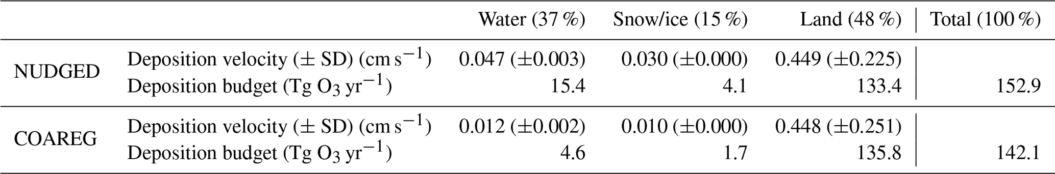
The temporal evolution in oceanic O₃ deposition velocities simulated by the COAREG run appears to be on the low side of observed $V_{\mathrm{d},{\mathrm{O}}_{\mathrm{3}}}$ and of that simulated elsewhere (e.g., Chang et al., 2004; Oh et al., 2008; Ganzeveld et al., 2009). Chang et al. (2004) showed that $V_{\mathrm{d},{\mathrm{O}}_{\mathrm{3}}}$ can increase by a factor of 5 with wind speed increasing from 0 to 20 m s⁻¹. Luhar et al. (2017) (their Fig. 7) shows a wide range of observed and simulated sensitivities to wind speed. Observations from the TexAQS06 summer campaign in the Gulf of Mexico show a large sensitivity to 10 m wind speeds even though the model seems unable to capture these high deposition velocities at high wind speeds (Luhar et al., 2017). However, Luhar et al. (2017) also shows that for the GasEx08 campaign in the cold Southern Ocean the sensitivity of observed and simulated $V_{\mathrm{d},{\mathrm{O}}_{\mathrm{3}}}$ to 10 m wind speeds is very limited. This limited sensitivity is most accurately represented by the modified two-layer reactivity scheme compared to the older one-layer scheme due to a more limited interaction between chemical reactivity and waterside turbulent transport (Luhar et al., 2017). Furthermore, the variability around the mean presented in Table 1 (0.012 ± 0.002 cm s⁻¹) seems to correspond to the Oh et al. (2008) (0.016 ± 0.0015 cm s⁻¹) 1-month simulation including O₃ removal by I${}_{\mathrm{aq}}^{-}$. In this study we show the intra-monthly variability in oceanic O₃ deposition, which is expected to be relatively low compared to the seasonal variability which will also be driven by temporal changes in solubility and reactivity due to the seasonal changes in SST and I${}_{\mathrm{aq}}^{-}$.

By estimating the total deposition flux for the water, snow/ice and land surfaces we can quantify the total simulated O₃ deposition budget (Table 1) for the Arctic modeling domain. Land, not covered with snow or ice, is the dominant surface type for this specific domain setup in summer with 48 %. Combined with a relatively high simulated $V_{\mathrm{d},{\mathrm{O}}_{\mathrm{3}}}$ of ∼ 0.45 cm s⁻¹, this is the most important sink, in terms of deposition, of simulated O₃ with ∼ 135 Tg O₃ yr⁻¹. The simulated O₃ deposition budget to water bodies, covering 37 % of the total surface area, contributes ∼ 10 % in the NUDGED run (15.4 Tg O₃ yr⁻¹) to the total O₃ deposition sink. In the COAREG run, this reduces to only ∼ 3 % (4.6 Tg O₃ yr⁻¹) of the total O₃ deposition sink. Simulated O₃ deposition to snow and ice, covering 15 % of the total surface area, is the least important deposition sink removing 4.1 and 1.7 Tg O₃ yr⁻¹ in the NUDGED and COAREG runs, respectively.

3.2 Simulated and observed monthly mean surface ozone

Figure 3 shows the spatial distribution in the simulated mean surface O₃ mixing ratios overlain with the observed mean surface O₃ mixing ratios. In the NUDGED and COAREG runs (Fig. 3a and b, respectively) we find similar surface O₃ mixing ratios of ∼ 15–20 ppb over the Russian, Canadian and Alaskan landmasses. Over Scandinavia, slightly higher surface O₃ mixing ratios of ∼ 20–25 ppb are simulated due to more anthropogenic emissions of precursors in the EDGAR emission inventory and advection of O₃ and its precursors from outside the domain. As expected, we find a limited effect of reduced deposition to water and snow/ice to the simulated mean O₃ mixing ratios over land. In general, the model appears to simulate the mean observed surface O₃ mixing ratios for the Remote and Terrestrial sites (all sites < 70^∘ N) generally well without clear positive or negative bias. Due to the altitude effect, relatively high surface O₃ concentrations are simulated over Greenland even though the deposition velocity to snow and the surrounding oceans is of similar magnitude (∼ 0.01 cm s⁻¹).

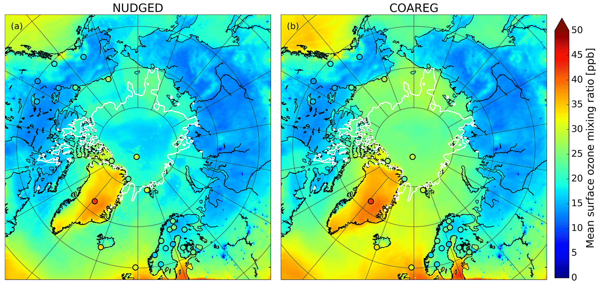
Figure 3 Spatial distribution of the simulated mean surface O₃ mixing ratio (ppb) for the (a) NUDGED and (b) COAREG runs. The filled circles indicate the mean observed ozone mixing ratios (ppb) for the simulated period. To indicate the sea ice extent, the white contours show the sea ice fraction of 0.5 at the start of the simulation.

The reduced O₃ deposition to water and snow/ice surfaces, comparing the NUDGED and COAREG simulation results (Sect. 3.1, Table 1), appears to be limited in terms of relative changes in $V_{\mathrm{d},{\mathrm{O}}_{\mathrm{3}}}$ and the total simulated O₃ deposition budget. However, these relatively small changes do substantially affect the simulated spatial distribution of surface O₃ mixing ratios over oceans and sea ice as indicated in Fig. 3. We find that the NUDGED run (Fig. 3a) systematically underestimates the mean observed surface O₃ mixing ratios for the High Arctic sites (all sites > 70^∘ N) by ∼ 5–10 ppb, which appears to be caused by an overestimated deposition to ocean, snow and ice surfaces, also further substantiated by the following analysis of temporal variability in O₃ concentrations (Sect. 3.3). Over the Arctic sea ice and oceans the ABL is typically very shallow and atmospheric turbulence is relatively weak. This suppresses vertical mixing and entrainment of O₃-rich air from the free troposphere. Dry deposition of O₃ to the ocean or snow/ice surfaces appears to be an important removal mechanism that has a large impact on O₃ concentrations in these shallow ABLs (Clifton et al., 2020b) both in terms of magnitude but also temporal variability (see Sect. 3.4). In the COAREG run, surface O₃ mixing ratios over oceans and Arctic sea ice have increased by up to 50 %. Furthermore, the reduced deposition to snow/ice has also clearly affected simulated surface O₃ mixing ratios over Greenland. Most importantly, the negative bias in simulated surface O₃ mixing ratios is reduced in the COAREG run with respect to the NUDGED run (see Sect. 3.3).

3.3 Simulated and observed hourly surface ozone

In this section we show how the application of the revised deposition scheme improves the model prediction scores of surface O₃ concentrations reflected in a comparison of the simulated and observed hourly surface O₃ mixing ratios at the three site selections (High Arctic, Remote and Terrestrial). To our knowledge, this is the first time such an oceanic O₃ deposition scheme coupled to a meteorology–chemistry model has been evaluated against a large dataset of hourly surface O₃ observations. Figure 4 shows a comparison between observed and simulated hourly surface O₃ mixing ratios subdivided into the three site selections: High Arctic, Remote and Terrestrial. As expected, for the High Arctic sites (Fig. 4, top row) we find that the NUDGED run is underestimating the observed surface O₃ mixing ratios with a mean bias of −3.8 ppb, which is also consistent with the findings in Fig. 3, where the NUDGED run appears to underestimate surface O₃ mixing ratios in the High Arctic region. The COAREG run, having a reduced O₃ deposition sink to oceans and snow/ice appears to better represent the surface O₃ observations with a slight positive bias of 0.3 ppb. The mean absolute error (MAE) in the COAREG run is reduced to 4.7 ppb from 6.4 ppb for the NUDGED run. Furthermore, we find that the CAMS reanalysis data also underestimate surface O₃ in the High Arctic with a bias of −5.0 ppb and an MAE of 6.8 ppb. Note that the performance for the WRF runs and CAMS reanalysis product varies for each observational site, which is further examined in Sect. 3.4.

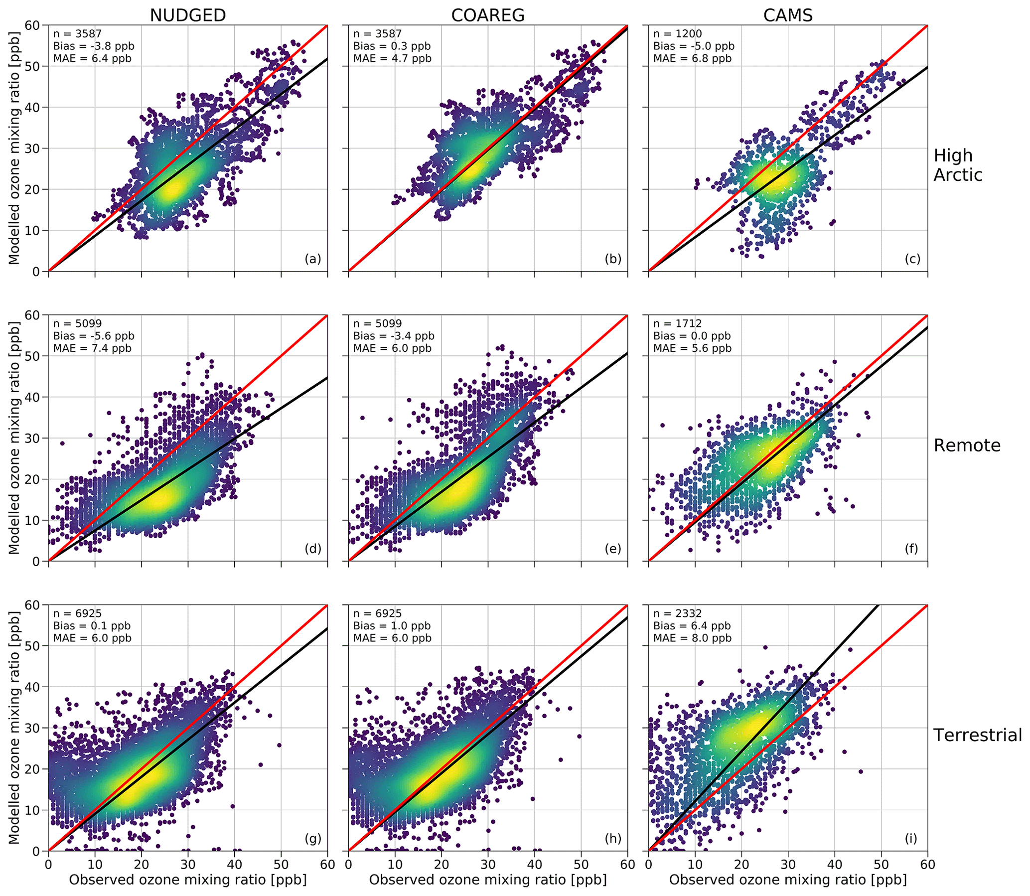
Figure 4 Comparison of the hourly observed and simulated ozone mixing ratios (ppb) for the NUDGED (a, d, g) and COAREG (b, e, h) runs and CAMS data (c, f, i) for the High Arctic (a–c), Remote (d–f) and Terrestrial (TE) (g–i) sites. The red line indicates the 1 : 1 line and the black line indicates the ordinary least squares regression line through the origin. The number of data points (n), bias (ppb) and mean absolute error (MAE) (ppb) are shown in the top left corner. The colors represent the multivariate kernel density estimation with yellow colors having a higher density.

For the Remote sites (Fig. 4, middle row), having no clear diurnal cycle in surface O₃, we again find an improvement by including the mechanistic ocean deposition routine and reduced snow/ice deposition. This improvement appears to be most pronounced for coastal sites like Stórhöfði (63.4^∘ N, 20.3^∘ W) and Inuvik (68.4^∘ N, 133.7^∘ W) with a reduction in the MAE of 32 % and 19 %, respectively (not shown here). Overall, the improvement for the COAREG compared to the NUDGED run in the Remote site selection is not as significant compared to the High Arctic sites, also because of the larger role of O₃ deposition to land and vegetation, which remained unchanged in this study. We find that the CAMS data show the best performance for the Remote sites with no bias and with an MAE of 5.6 ppb.

For the Terrestrial sites (Fig. 4, bottom row), having a clear diurnal cycle in surface O₃, the WRF runs slightly overestimate the observed surface O₃ mixing ratios with mean biases of 0.1 and 1.0 ppb for the NUDGED and COAREG runs, respectively. Reducing the O₃ deposition to oceans and snow/ice increases the bias, but the MAE of 6.0 ppb remains unchanged. The CAMS reanalysis data appear to perform worst for the Terrestrial sites with a bias of 6.4 ppb and an MAE of 8.0 ppb. This might be explained by the lower spatial and temporal resolution of CAMS specifically at these sites having a relatively strong diurnal cycle in ABL dynamics, O₃ deposition to vegetation and O₃ concentrations. Also a misrepresentation of emissions of precursor emissions and concentrations and the O₃ deposition to vegetation (Michou et al., 2005; Val Martin et al., 2014) might explain some of the differences.

3.4 Temporal variability of surface ozone in the High Arctic

In Sect. 3.3 we have shown how revising the O₃ deposition scheme to oceans and snow/ice can improve the model's capability to represent the observed hourly surface O₃ mixing ratios, especially for the High Arctic sites. In this section we show how the NUDGED and COAREG runs and CAMS represent the temporal variation in High Arctic surface O₃ observations, focusing on 6 out of the 25 measurement sites. These six High Arctic sites have been selected due to their deposition footprint being dominated by transport over, and deposition to, ocean and sea-ice-covered surfaces. Figure 5 shows the observed and simulated surface O₃ time series for ASCOS, Summit, Villum, Zeppelin, Barrow and Alert. Furthermore, Table 2 shows the model skill indicators for the High Arctic sites. These skill indicators include the mean absolute error (MAE) that represents the systematic error, the standard deviation of observation minus model prediction σ_o−p that represents the random error, and the Pearson R correlation coefficient (R) that represents the degree of correlation.

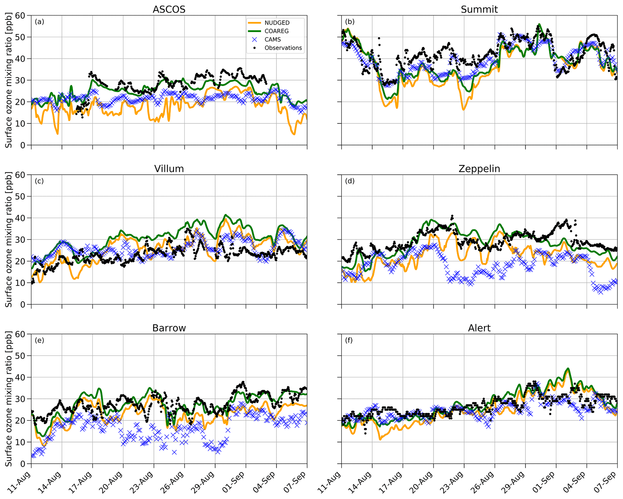
Figure 5 Temporal evolution of hourly surface O₃ mixing ratios (ppb) for the NUDGED (yellow) and COAREG (green) runs, CAMS data (blue crosses) and observations (black dots) at ASCOS (∼ 87.4^∘ N, ∼ 6.0^∘ W), Summit (72.6^∘ N, 38.5^∘ W), Villum (81.6^∘ N, 16.7^∘ W), Zeppelin (78.9^∘ N, 11.9^∘ E), Barrow (71.3^∘ N, 156.6^∘ W) and Alert (82.5^∘ N, 62.3^∘ W).

Table 2 MAE (ppb), σ_o−p (ppb) and Pearson R correlation coefficient (R) (–) for the NUDGED and COAREG runs and CAMS reanalysis data at the ASCOS, Summit, Villum, Zeppelin, Barrow and Alert observational sites. The lowest model error and highest correlation have been made bold for every site.

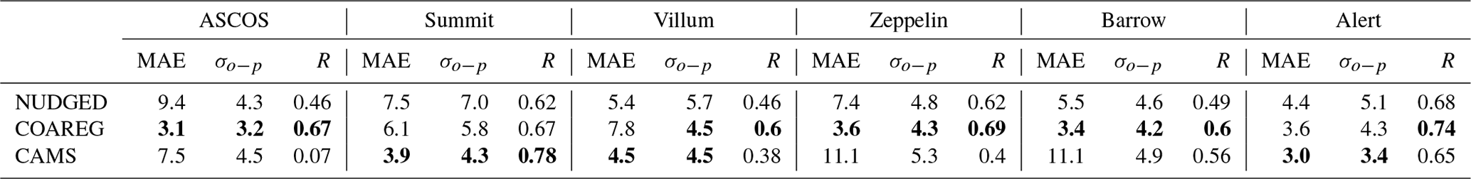
The observations at ASCOS (Fig. 5a) show a sudden increase in surface O₃ mixing ratios from 20 to over 30 ppb around the 17 August due to advection of relatively O₃-rich air during a synoptically active period (Tjernström et al., 2012). Only the COAREG run appears to be able to simulate a similar increase in surface O₃, while NUDGED and CAMS show a minor increase in simulated surface O₃. From the 17 August onwards, the observations show mixing ratios between 25 and 35 ppb. The WRF simulations indicate advection of air over ocean and ice surfaces during this time period (not shown here). In the COAREG simulation, with less deposition to these surfaces, surface O₃ mixing ratios are less depleted. Only the COAREG run is able to represent these observed mixing ratios with a bias of −2.0 ppb, whereas NUDGED and CAMS are clearly biased towards lower mixing ratios.

At Summit (Fig. 5b), we find a large temporal variability in observed surface O₃ between 30 and 55 ppb. From the 11 August onwards we find a decreasing trend in observed surface O₃ down to 30 ppb before increasing to 40 ppb around the 17 August. All models capture this specific event in terms of temporal variability even though NUDGED and COAREG are still biased at the observed minimum of 30 ppb. Furthermore, we find that the CAMS reanalysis data represent this specific period very well, also in terms of magnitude. At Summit, the increase in surface O₃ in the COAREG run relative to the NUDGED run mostly reflects the reduction in deposition to snow and ice due to the prevailing katabatic wind flow (Gorter et al., 2014). During episodes with low wind speeds the ABL becomes very stable and shallow during which deposition to snow and ice becomes an important process in removing O₃ in the ABL. In the period between the 14 and 26 August this reduction in deposition can increase the surface O₃ mixing ratios of up to 10 ppb (e.g., 23 August). In contrast, during episodes with higher wind speeds and deeper ABLs the reduced O₃ deposition to snow hardly affects the simulated surface O₃ concentrations. Interestingly, we find that the NUDGED and COAREG simulations show a larger negative bias (∼ 5–10 ppb) during the period with low wind speeds and shallow ABLs. Over the entire simulated period, CAMS performs best at Summit, with an MAE of 3.9 ppb, followed by COAREG, with an MAE of 6.1 ppb.

Villum (Fig. 5c) is the only site for which the NUDGED and COAREG runs as well as the CAMS reanalysis data all systematically overestimate the observed mixing ratios, especially later into the simulation. The observations show an increase in O₃ mixing ratios from 10 to 20 ppb in the first 3 d of the simulation, whereafter it remains between 20 and 30 ppb with relatively low temporal variability compared to some of the other sites (e.g., Summit, Barrow). Both the NUDGED and COAREG runs simulate mixing ratios of up to 40 ppb, and CAMS simulates maximum surface O₃ mixing ratios of 35 ppb. In terms of representing the magnitude of surface O₃ mixing ratios CAMS performs best with an MAE of 4.5.

Zeppelin (Fig. 5d) and Barrow (Fig. 5e) show similar behavior in terms of observation–model comparison. For both locations the CAMS reanalysis data systematically underestimate observed O₃ mixing ratios with a biases > 10 ppb. In the NUDGED run the bias equals −6.9 and −4.6 ppb for Zeppelin and Barrow, respectively. In the COAREG run the bias is reduced to −1.0 and −0.2 ppb for Zeppelin and Barrow, respectively. This reduction in bias is, together with ASCOS, the largest among the six High Arctic sites and shows the large sensitivity to the representation of O₃ deposition. At Barrow, the dominant wind directions during the simulation period are NW–NE reflecting a footprint mostly from the Arctic sea ice and ocean. Especially in the period from the 23 August onward, the COAREG run is very accurate in representing the magnitude as well as the temporal variability in observed surface O₃. During this period, the NUDGED run simulates surface O₃ mixing ratios of up to 5 ppb lower due to the overestimated deposition to oceans and sea ice. At both sites, the model performance of COAREG is in the same order of magnitude, with an MAE, σ_o−p and R of 3.5 ppb, 4.2 ppb and 0.65, respectively.

At Alert (Fig. 5f), we find a relatively steady increase in observed surface O₃ from 20 ppb at the start of the simulation to 30 ppb at the end of the simulation. The temporal variability, both in observed and simulated surface O₃, appears to be lower compared to some of the other High Arctic sites. Again, the statistical parameters such as MAE, σ_o−p and R improve in the COAREG run with respect to the NUDGED run. At Alert, we find that CAMS has the lowest MAE and σ_o−p of 3.0 and 3.4 ppb, respectively.

The model performance in terms of temporal variability in surface O₃ observations is diagnosed by using the Pearson R correlation coefficient. The model performance improved for all six sites in the COAREG run with respect to the NUDGED run. The COAREG simulation performs best for five out of the six observational sites in terms of Pearson R correlation coefficient and is only outperformed by CAMS at Summit. Overall, we find that coupling the WRF model to the mechanistic COAREG ocean–atmosphere exchange representation decreases the MAE and σ_o−p for all High Arctic sites except for Villum by better representing the magnitude of, but also temporal variability in observed surface O₃. The CAMS reanalysis data perform well for some locations (e.g., Summit, Alert), while for Zeppelin and Barrow the discrepancy is among the largest we found in the observation–model comparison.

4 Discussion

This study demonstrates the impact of a mechanistic representation of ocean–atmosphere O₃ exchange to simulate the magnitude and temporal variability of hourly surface O₃ concentrations in the Arctic at 25 sites. We show that the modeled sensitivity of the surface O₃ concentrations to the representation of O₃ to ocean, ice and snow surfaces is high, even though the total deposition budget is an order of magnitude smaller than the deposition budget to land and vegetation. Using a mechanistic oceanic O₃ deposition representation and reduced O₃ deposition to snow and ice greatly reduced the negative bias in surface O₃, especially in the High Arctic. Furthermore, the temporal variability in surface O₃ was also better represented by the mechanistic representation of oceanic O₃ deposition also accounting for temporal variations in the driving processes of oceanic O₃ deposition such as waterside turbulent transport. This analysis also shows a discrepancy in the representation of simulated O₃ at sites having a terrestrial footprint (e.g., Norway, Sweden, Finland). However, the model representation of O₃ deposition to vegetation and land, including diurnal and seasonal variability (Lin et al., 2019), is beyond the scope of this study. To find out whether the implementation of a mechanistic representation of oceanic O₃ deposition specifically affects the variability of surface O₃ at certain timescales, we have performed an additional wavelet analysis (Torrence and Compo, 1998). For the six High Arctic sites we found that ∼ 55 %–70 % of the simulated and observed signal is present at timescales > 4 d representing the longer timescales and synoptic variability in wind speeds and vertical and horizontal mixing conditions. Interestingly, we found that the observations show more variability compared to the model simulations at timescales of hours, arguably due to the misrepresentation of some sub-grid processes. We do not find any clear indication that the implementation of COAREG significantly affects the variability of surface O₃ at High Arctic sites at a specific timescale.

The COAREG scheme has been developed and validated against eddy-covariance measurements over mostly subtropical waters (Bariteau et al., 2010; Helmig et al., 2012) and has been applied to study the effects of wind speed and sea state on ocean–atmosphere gas transfer (Blomquist et al., 2017; Bell et al., 2017; Porter et al., 2020). We do expect that these main drivers, i.e., waterside turbulent transfer and chemical enhancement with dissolved iodide, also control oceanic O₃ deposition at high latitudes. Indirect evaluation of oceanic O₃ deposition through a comparison of surface O₃ observations instead of direct oceanic O₃ flux measurements indicates that including this mechanistic representation of O₃ deposition improves both the modeled magnitude and temporal variability in surface O₃ observations. However, a lack of oceanic O₃ deposition flux measurements hampers the direct model evaluation of the high-latitude O₃ deposition flux. This is expected to be soon resolved by getting access to O₃ flux observations collected in the Multidisciplinary drifting Observatory for the Study of Arctic Climate (MOSAiC) 1-year field campaign.

Furthermore, we have reduced the deposition to snow and ice following Helmig et al. (2007a) and Clifton et al. (2020a). The results of Helmig et al. (2007a) also motivated follow-up observational and modeling studies aiming at the development of more mechanistic representations of O₃ deposition to snow-/ice-covered surfaces. For example, efforts have been made to simulate O₃ dynamics in and above the snowpack using a 1D model setup to explain observations of O₃ and NO_x concentrations measured above and inside the Summit snowpack (Van Dam et al., 2015). This 1D modeling study suggested the role of aqueous-phase oxidation of O₃ with formic acid in the snowpack (Murray et al., 2015). Comparable 1D modeling studies focused on assessing the role of catalytic O₃ loss via bromine radical chemistry in the snowpack interstitial air (Thomas et al., 2011; Toyota et al., 2014). However, these studies mainly addressed the role of some of this snowpack chemistry in explaining, partly observed, O₃ concentrations and not so much on snow–atmosphere O₃ fluxes and derived deposition rates that would corroborate the inferred very small O₃ deposition rates by Helmig et al. (2007a). Clifton et al. (2020a) summarized that accurate process-based modeling of O₃ deposition to snow requires a better understanding of the underlying processes and dependencies. An eddy-covariance system that has been deployed as part of the MOSAiC campaign will further enhance our understanding of O₃ deposition in shallow ABLs at high latitudes (Clifton et al., 2020b).

In this study we used the COAREG transfer algorithm version 3.6, which is extended with a two-layer scheme for surface resistance compared to the previous versions (Fairall et al., 2007, 2011) and is similar to Luhar et al. (2018). Our WRF simulations excluded the additional role of chlorophyll, dissolved organic matter (DOM) or other species such as DMS on chemical enhancement of O₃ in surface waters. Experimental studies have shown that DMS, chlorophyll or other reactive organics may enhance the removal of O₃ at the sea surface (Chang et al., 2004; Clifford et al., 2008; Reeser et al., 2009; Martino et al., 2012). The global modeling study by Ganzeveld et al. (2009) included a chlorophyll–O₃ reactivity that increased linearly with chlorophyll concentration as a proxy for the role of DOM in oceanic O₃ deposition. Including this reaction substantially enhances O₃ deposition to coastal waters such that actually observed O₃ deposition to these coastal waters is well reproduced (Ganzeveld et al., 2009). Other studies such as Luhar et al. (2017) and Pound et al. (2020) ignored the potential role of DOM–O₃ chemistry in oceanic O₃ deposition. Luhar et al. (2018), who did not explicitly consider coastal waters, even suggested that including such a reaction deteriorates the comparison with O₃ flux observations above open oceans. To test the sensitivity of our model setup to other reactants in the surface water we have performed an additional sensitivity analysis including the chlorophyll–O₃ and DMS–O₃ reactions from Ganzeveld et al. (2009). Oceanic chlorophyll concentrations have been retrieved from the 9 × 9 km resolution MODIS chlorophyll-α dataset available at https://modis.gsfc.nasa.gov/data/dataprod/chlor_a.php (last access: 14 August 2020). Chlorophyll-α concentrations are typically < 3 mg m⁻³ for open oceans and up to 25 mg m⁻³ for coastal waters. For oceanic DMS concentrations, we use the monthly climatology from Lana et al. (2011). The sensitivity study with chlorophyll as an additional reactant indicated a slight increase (up to 5 %) in deposition to coastal waters with chlorophyll concentrations of up to 25 mg m⁻³. However, the resulting effect on surface O₃ concentrations was not significant due to the large fraction of oceans with very low (< 3 mg m⁻³) chlorophyll-α concentrations. Also, the reactions with oceanic DMS appear to be weak due to relatively low DMS concentrations in August/September. These sensitivity studies indicate that I${}_{\mathrm{aq}}^{-}$ is the main driver of chemical reactivity of O₃ in the Arctic Ocean in summer. However a potential sensitivity of these reactants on Arctic O₃ deposition could be expected especially in the spring to summer transition following algal blooms (Stefels et al., 2007; Riedel et al., 2008).

We nudged the WRF model to the ECMWF ERA5 reanalysis product to ensure a fair model evaluation with observations due to a better representation of the synoptic conditions. This indicated the important role of the model representation of meteorology, e.g., the advection of polluted air and mixing/entrainment of O₃ in the ABL, in representing the observed surface O₃ concentrations. The model evaluation was set up at a resolution of 30 × 30 km, which is in the order of the ERA5 reanalysis data (0.25^∘ × 0.25^∘) used for initial conditions, boundary conditions and nudging. Here, we opted for a 30 km grid spacing because we expect that the main drivers of tropospheric O₃ (chemical production and destruction, stratosphere–troposphere transport, dry deposition, mixing and advection processes) can be sufficiently resolved at this grid spacing especially over the relatively homogeneous ocean, ice and snow surfaces. However, we do realize that such a coarse grid spacing may have hampered representing local air flow phenomena such as katabatic winds (Klein et al., 2001), which could explain some of the mismatch at sites like Villum (Nguyen et al., 2016). Another justification for the 30 km grid spacing was to limit computational time and to have a large enough domain to cover the entire region above 60^∘ N to conduct a large pan-Arctic evaluation while at the same time having all observational sites far enough from the domain boundaries to limit the effect of the imposed meteorological and chemical boundary conditions.

In general, the relatively scarce Arctic observations limit evaluation of modeling studies and extrapolation of these results for the Arctic summer to other seasons and lower latitudes. In this case, this includes the uncertainty in the magnitude and distribution of driving factors of oceanic O₃ deposition such as I${}_{\mathrm{aq}}^{-}$ or DOM. New I${}_{\mathrm{aq}}^{-}$ measurements at high latitudes, for example those performed during the year-round MOSAiC expedition, will be very useful to better constrain the global I${}_{\mathrm{aq}}^{-}$ distributions as well as mechanistic oceanic O₃ deposition representations. Measurements of O₃ concentrations and deposition fluxes to the Arctic Ocean can assist us to better constrain these modeling setups in terms of magnitude and temporal variability and can potentially indicate the sensitivity to other environmental factors such as wind speed in waters with low reactivity. Furthermore, including the role of halogen chemistry (Pratt et al., 2013; Thompson et al., 2017) might give an indication of the combined role of halogens and oceanic deposition in removing O₃ and explaining the magnitude and temporal variability of O₃ concentrations in the High Arctic.

5 Conclusions

The mesoscale meteorology–chemistry model Polar-WRF-Chem was coupled to the Coupled Ocean-Atmosphere Response Experiment Gas transfer algorithm (COAREG) to allow for a mechanistic representation of ocean–atmosphere exchange of O₃. This scheme represents the effects of molecular diffusion, solubility, waterside turbulent transfer and chemical enhancement of O₃ uptake through its reactions with dissolved iodide. The COAREG scheme replaces the constant surface uptake resistance approach often applied in ACTMs. Furthermore, we have increased the modeled O₃ surface uptake resistance to snow and ice. In total, two simulations were performed: (1) a default WRF setup nudged to ERA5 synoptic conditions (NUDGED) and (2) a WRF setup with adjustments to O₃ surface uptake resistance as described above (COAREG). Furthermore, the CAMS global reanalysis data product has also been included in the presented evaluation of High Arctic surface O₃. This CAMS product is widely used in air quality assessments and to constrain regional-scale modeling experiments. This provides additional information on the quality of the CAMS data products but also on potential issues in the representation of O₃ sources and sinks, e.g., oceanic and snow/sea ice deposition, for the High Arctic. The modeling approach was set up for 1 month at the end of summer 2008 and evaluated against hourly surface O₃ at 25 sites for latitudes > 60^∘ N including observations over the Arctic sea ice as part of the ASCOS campaign.

Using the mechanistic representation of ocean–atmosphere exchange, O₃ deposition velocities were simulated in the order of 0.01 cm s⁻¹ compared to ∼ 0.05 cm s⁻¹ in the constant surface uptake resistance approach. In the COAREG run, the spatial variability (0.01 to 0.018 cm s⁻¹) in the mean O₃ deposition velocities expressed the sensitivity to chemical enhancement with dissolved iodide. The temporal variability of O₃ deposition velocities (up to ±20 % around the mean) is governed by surface wind speeds and expressed differences in waterside turbulent transport. Using the mechanistic representation of ocean–atmosphere exchange reduced the total simulated O₃ deposition budget to water bodies by a factor of 3.3 compared to the default constant ocean uptake rate approach and the increase in surface uptake resistance to snow and ice reduced the deposition budget by a factor of 2.4.

Despite the fact that O₃ deposition to oceans, snow and ice surfaces only constitutes a small term in the total O₃ deposition budget (> 90 % of the deposition is to land), we find a substantial sensitivity to the simulated surface O₃ mixing ratios. In the COAREG run, the simulated mean monthly surface O₃ mixing ratios have increased by up to 50 % in the typically shallow Arctic ABL above the oceans and sea ice relative to the NUDGED run. The mechanistic representation of O₃ deposition to oceans resulted in a substantially improved representation of surface O₃ observations, especially for the High Arctic sites with latitudes > 70^∘ N. The NUDGED run underestimated the observed surface O₃ mixing ratios with a bias of −3.8 ppb, whereas the COAREG run had a bias of 0.3 ppb. The evaluation of the WRF runs at individual High Arctic sites showed that using the mechanistic representation of O₃ deposition to oceans results in a better representation of surface O₃ observations both in terms of magnitude and temporal variability. Similar to the NUDGED run, CAMS underestimated High Arctic observed surface O₃ with a bias of −5.0 ppb indicating that the representation of the deposition removal mechanism to oceans and snow/ice in CAMS might also be overestimated and should be reconsidered.

This study highlights the impact of a mechanistic representation of oceanic O₃ deposition on Arctic surface O₃ concentrations at a high (hourly) temporal resolution. It mostly corroborates the findings of global-scale studies (e.g., Ganzeveld et al., 2009; Luhar et al., 2017; Pound et al., 2020) and recommends that the representation of O₃ deposition to oceans and snow/ice in global- and regional-scale ACTMs should be revised. This revision is needed not only to better quantify the O₃ budget at the global scale, but also to better represent the observed magnitude and temporal variability of surface O₃ at the regional scale. In addition, explicit consideration of the mechanisms involved in O₃ removal by the oceans (and sea ice/snowpack) are essential to also evaluate the role of potentially important feedback mechanisms and future trends in and the role of O₃ in Arctic climate change as a function of declining sea ice cover, increasing emissions and changes in oceanic biogeochemical conditions. On the regional scale, this study also has implications for methods to quantify future trends in Arctic tropospheric O₃, Arctic air pollution and climate in a period of declining sea ice and increasing local emissions of precursors.

Appendix A: WRF physical and chemical parameterization schemes.

(Hong et al., 2004)(Iacono et al., 2008)(Iacono et al., 2008)(Janjić, 2001)(Chen and Dudhia, 2001)(Janjić, 1994)(Kain, 2004)Gery et al., 1989Zaveri and Peters, 1999(Wild et al., 2000)(Janssens-Maenhout et al., 2019)(Guenther et al., 2012)(Hersbach et al., 2020)(Inness et al., 2019)

Table A1 WRF physical and chemical parameterization schemes.

Appendix B: Formulation of the air side and waterside resistance terms

The exchange velocity, in this case deposition, of ozone ($V_{\mathrm{d},{\mathrm{O}}_{\mathrm{3}}}$) (m s⁻¹) is calculated from the waterside resistance (r_w) (s m⁻¹) and air side resistance terms (r_a+r_b) (s m⁻¹) as follows:

$$\begin{array}{}\text{(B1)}& V_{\mathrm{d},{\mathrm{O}}_{\mathrm{3}}}={\displaystyle \frac{\mathrm{1}}{\mathit{\alpha }{r}_{\mathrm{w}}+r_{\mathrm{a}}+r_{\mathrm{b}}}}.\end{array}$$

Here, α (–) is the dimensionless solubility of O₃ in sea water calculated from SST (K) following Morris (1988) as

$$\begin{array}{}\text{(B2)}& \mathit{\alpha }={\mathrm{10}}^{-\mathrm{0.25}-\mathrm{0.013}(\mathrm{SST}-\mathrm{273.16})},\end{array}$$

and the waterside resistance term (r_w) is calculated as

$$\begin{array}{}\text{(B3)}& r_{\mathrm{w}}=(a\cdot D{)}^{-\mathrm{1}/\mathrm{2}}{\displaystyle \frac{\mathrm{\Psi }{K}_{\mathrm{1}}\left({\mathit{\xi }}_{\mathit{\delta }}\right)\sinh \mathit{\lambda }+K_{\mathrm{0}}\left({\mathit{\xi }}_{\mathit{\delta }}\right)\cosh \mathit{\lambda }}{\mathrm{\Psi }{K}_{\mathrm{1}}\left({\mathit{\xi }}_{\mathit{\delta }}\right)\cosh \mathit{\lambda }+K_{\mathrm{0}}\left({\mathit{\xi }}_{\mathit{\delta }}\right)\sinh \mathit{\lambda }}}.\end{array}$$

Here, a (s⁻¹) is the chemical reactivity of O₃ with I${}_{\mathrm{aq}}^{-}$ calculated with the second-order rate coefficient (M⁻¹ s⁻¹) from Magi et al. (1997) and the I${}_{\mathrm{aq}}^{-}$ concentrations (M) from Sherwen et al. (2019):

$$\begin{array}{}\text{(B4)}& a=k\cdot \left[I_{\mathrm{aq}}^{-}\right]=\exp \left({\displaystyle \frac{-\mathrm{8772.2}}{\mathrm{SST}}}+\mathrm{51.5}\right)\cdot \left[I_{\mathrm{aq}}^{-}\right].\end{array}$$

In Eq. (B3), D (m² s⁻¹) is the molecular diffusivity of O₃ in ocean water and is calculated from the kinematic viscosity ν (m² s⁻¹) and the waterside Schmidt number (S_cw) (–) as

$$\begin{array}{}\text{(B5)}& D={\displaystyle \frac{\mathit{\nu }}{S_{\mathrm{cw}}}}={\displaystyle \frac{\mathit{\mu }}{\mathit{\rho }}}/\left[\sqrt{\mathrm{44}/\mathrm{48}}\cdot \exp \left(-\mathrm{0.055}\cdot \mathrm{SST}+\mathrm{22.63}\right)\right],\end{array}$$

where μ (kg m⁻¹ s⁻¹) is the dynamic viscosity of seawater and ρ (kg m⁻³) is the density of seawater.

Finally, the air side resistance terms (r_a+r_b) (s m⁻¹) of the deposition velocity in Eq. (B1) are calculated as

$$\begin{array}{}\text{(B6)}& r_{\mathrm{a}}+r_{\mathrm{b}}=\left[C_{\mathrm{d}}^{-\mathrm{1}/\mathrm{2}}+\mathrm{13.3}{S}_{\mathrm{c}}^{\mathrm{1}/\mathrm{2}}-\mathrm{5}+{\displaystyle \frac{\log \left(S_{\mathrm{c}}\right)}{\mathrm{2}\mathit{\kappa }}}\right]/u_{*,\mathrm{a}},\end{array}$$

where C_d (–) is the momentum drag coefficient, S_ca (–) is the Schmidt number for ozone in the atmosphere, κ is the von Kármán constant (0.4) and $u_{*,\mathrm{a}}$ (m s⁻¹) is the friction velocity in the atmosphere. The r_a+r_b term is typically in the order of 100 s m⁻¹ (Fairall et al., 2011).

Compared to COAREG version 3.1 (Fairall et al., 2007, 2011), COAREGv3.6 is extended with a two-layer scheme based on Luhar et al. (2018). This extension is included in the second term of the waterside resistance term (Eq. B3). Here, $\mathrm{\Psi }=\sqrt{\mathrm{1}+(\mathit{\kappa }{u}_{*,\mathrm{w}}{\mathit{\delta }}_m/D)}$, ${\mathit{\xi }}_{\mathit{\delta }}=\sqrt{\mathrm{2}ab({\mathit{\delta }}_m+bD/\mathrm{2})}$ and $\mathit{\lambda }={\mathit{\delta }}_m\sqrt{a/D}$ with $b=\mathrm{2}/\left(\mathit{\kappa }{u}_{*,\mathrm{w}}\right)$. This part of the equation is a function of the chemical reactivity a (s⁻¹) (Eq. B4), the waterside friction velocity $u_{*,\mathrm{w}}$ (m s⁻¹), the molecular diffusivity of O₃ in ocean water (Eq. B5) and δ_m (m) representing the depth of the interface between the top water layer and the underlying turbulent layer. In this study we have applied ${\mathit{\delta }}_m=c_{\mathrm{0}}\sqrt{D/a}$ with c₀=0.4 based on Luhar et al. (2018). K₀(ξ_δ) and K₁(ξ_δ) are the modified Bessel functions of the second kind of order 0 and 1, respectively. For more information on the derivation of the formulas, please visit Fairall et al. (2007, 2011) and Luhar et al. (2018).

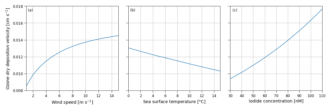
Figure B1 Sensitivity of the ozone dry-deposition velocity from COAREG to the environmental factors 10 m wind speed (m s⁻¹) (a), sea surface temperature (^∘C) (b) and sea surface iodide concentration (nM) (c) using typical values of 10 m wind speed, sea surface temperature and iodide concentration of 5 m s⁻¹, 5 ^∘C and 60 nM, respectively. Note that the sensitivity to sea surface temperature does not include effects of increasing reactivity but mostly represents the effect of reduced solubility (Eq. B2).

Figure B1 shows the sensitivity of the COAREG routine coupled to WRF to the environmental factors wind speed, SST and iodide concentration. The sensitivity to wind speeds (Fig. B1a) expresses the role of waterside turbulent transport and aerodynamic resistance. For low wind speeds waterside turbulent transport is limited and therefore limits the exchange of O₃ from the atmosphere to the ocean. At high wind speeds, the dry deposition of O₃ is limited by chemical reactivity of O₃ with I${}_{\mathrm{aq}}^{-}$ at typical Arctic SSTs of 5 ^∘C and I${}_{\mathrm{aq}}^{-}$ concentrations of 60 nM (see also Fig. C1). At very low wind speeds (< 2.5 m s⁻¹) the aerodynamic resistance poses an extra restriction on the ocean–atmosphere exchange of O₃. The sensitivity to SST (Fig. B1b) mostly represents the role of solubility (Eq. B2) with warmer waters having a lower solubility. In contrast to Luhar et al. (2018), the SST is not used to calculate the I${}_{\mathrm{aq}}^{-}$ concentrations and does therefore not show a positive correlation. The sensitivity to I${}_{\mathrm{aq}}^{-}$ (Fig. B1c) represents the role of chemical enhancement which is stronger than the generally compensating effect of solubility in warmer waters for typical Arctic conditions.

Appendix C: Spatial distribution of oceanic iodide

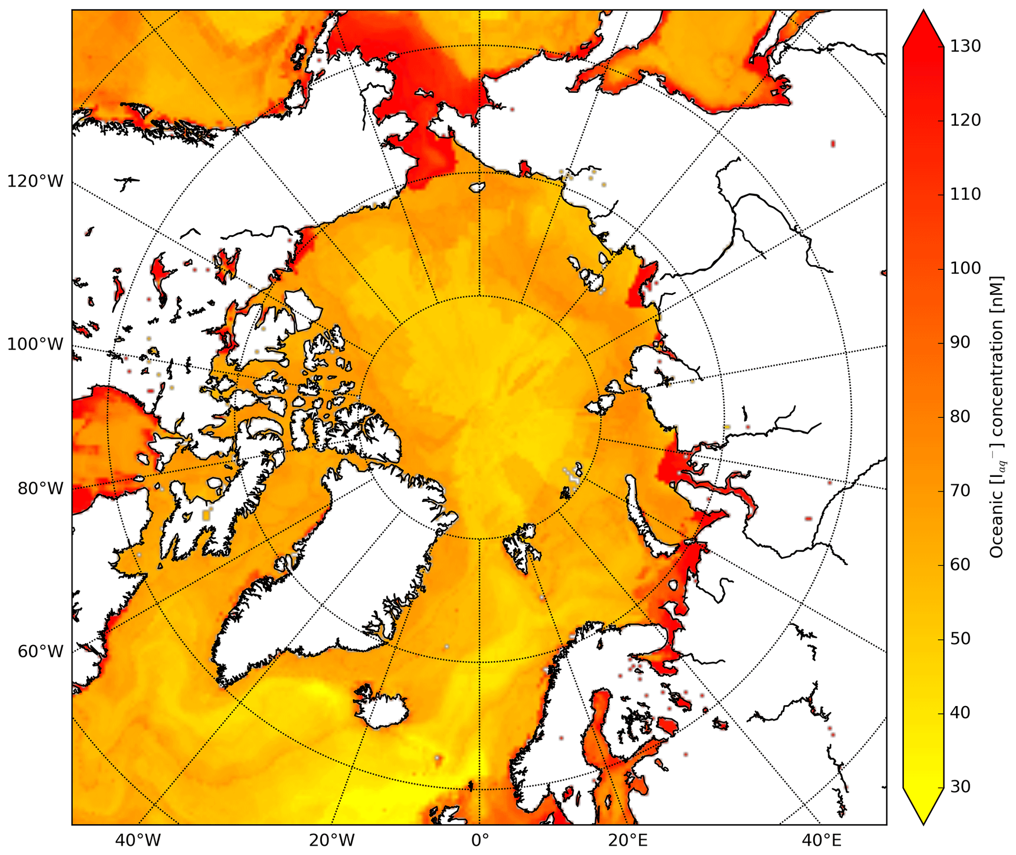
Figure C1 Spatial distribution of Sherwen et al. (2019) oceanic iodide concentrations (nM) at the start of the simulation.

Appendix D: Surface ozone measurement sites

Table D1 Surface ozone measurement sites subdivided in the“High Arctic”, “Remote” and “Terrestrial” site selections.