the Creative Commons Attribution 4.0 License.
the Creative Commons Attribution 4.0 License.
 | 12 Aug 2020
Evaluation of nitrogen oxides (NOx) sources and sinks and ozone production in Colombia and surrounding areas
Johannes G. M. Barten
Laurens N. Ganzeveld
Auke J. Visser
Rodrigo Jiménez
Maarten C. Krol
In Colombia, industrialization and a shift towards intensified agriculture have led to increased emissions of air pollutants. However, the baseline state of air quality in Colombia is relatively unknown. In this study we aim to assess the baseline state of air quality in Colombia with a focus on the spatial and temporal variability in emissions and atmospheric burden of nitrogen oxides (NOx = NO + NO2) and evaluate surface NOx, ozone (O3) and carbon monoxide (CO) mixing ratios. We quantify the magnitude and spatial distribution of the four major NOx sources (lightning, anthropogenic activities, soil biogenic emissions and biomass burning) by integrating global NOx emission inventories into the mesoscale meteorology and atmospheric chemistry model, namely Weather Research and Forecasting (WRF) coupled with Chemistry (collectively WRF-Chem), at a similar resolution (∼25 km) to the Emission Database for Global Atmospheric Research (EDGAR) anthropogenic emission inventory and the Ozone Monitoring Instrument (OMI) remote sensing observations. The model indicates the largest contribution by lightning emissions (1258 Gg N yr−1), even after already significantly reducing the emissions, followed by anthropogenic (933 Gg N yr−1), soil biogenic (187 Gg N yr−1) and biomass burning emissions (104 Gg N yr−1). The comparison with OMI remote sensing observations indicated a mean bias of tropospheric NO2 columns over the whole domain (WRF-Chem minus OMI) of 0.02 (90 % CI: [−0.43, 0.70]) ×1015 molecules cm−2, which is <5 % of the mean column. However, the simulated NO2 columns are overestimated and underestimated in regions where lightning and biomass burning emissions dominate, respectively. WRF-Chem was unable to capture NOx and CO urban pollutant mixing ratios, neither in timing nor in magnitude. Yet, WRF-Chem was able to simulate the urban diurnal cycle of O3 satisfactorily but with a systematic overestimation of 10 parts per billion (ppb) due to the equally large underestimation of NO mixing ratios and, consequently, titration. This indicates that these city environments are in the NOx-saturated regime with frequent O3 titration. We conducted sensitivity experiments with an online meteorology–chemistry single-column model (SCM) to evaluate how WRF-Chem subgrid-scale-enhanced emissions could explain an improved representation of the observed O3, CO and NOx diurnal cycles. Interestingly, the SCM simulation, showing especially a shallower nocturnal inversion layer, results in a better representation of the observed diurnal cycle of urban pollutant mixing ratios without an enhancement in emissions. This stresses that, besides application of higher-resolution emission inventories and model experiments, the diurnal cycle in boundary layer dynamics (and advection) should be critically evaluated in models such as WRF-Chem to assess urban air quality. Overall, we present a concise method to quantify air quality in regions with limited surface measurements by integrating in situ and remote sensing observations. This study identifies four distinctly different source regions and shows their interannual and seasonal variability during the last 1.5 decades. It serves as a base to assess scenarios of future air quality in Colombia or similar regions with contrasting emission regimes, complex terrain and a limited air quality monitoring network.
- Article
(2114 KB) - Full-text XML
- BibTeX
- EndNote


Nitrogen oxides (NOx = NO + NO2) are one of the main precursors of lower atmospheric ozone (O3). Exposure to NOx has an adverse effect on human health on an acute and long-term basis (Panella et al., 2000; Wolfe and Patz, 2002). In addition, O3 is toxic to humans (WHO, 2003) and can also reduce agricultural yields (Ashmore and Marshall, 1998). Therefore, accurate monitoring and predictions of surface concentrations of these air pollutants are key. Especially in densely populated regions, air pollution has been a major concern and is expected to even have larger impacts in the future due to the continuous urbanization and increasing emissions from, for example, traffic.
Anthropogenic NOx is produced in combustion processes and is an indicator of industrial activity and transportation and other anthropogenic activities like biomass burning and agricultural activities. Anthropogenic sources add up to ∼70 % (∼50 % industrial activity or transportation and ∼20 % biomass burning) of the total global annual NOx emissions (Lamarque et al., 2010). In addition to anthropogenic sources, natural sources contribute to total nitrogen budgets. NO emissions from soils add up to ∼12 %–20 % of the global NOx emissions on a yearly basis (Bradshaw et al., 2000; Ganzeveld et al., 2002a; Jaeglé et al., 2005; Vinken et al., 2014). Lightning emissions are estimated to contribute, on average, 10 %–18 % to the global yearly NOx emissions (Pickering et al., 2016). In the tropics (35∘ N–35∘ S), anthropogenic activities (7.81 Tg N yr−1), biomass burning (8.28 Tg N yr−1), soil emissions (5.44 Tg N yr−1) and lightning discharges (6.33 Tg N yr−1) all contribute an approximately equal fraction to the total NOx emission budget (Bond et al., 2002). A modeling study in the tropics must therefore provide accurate estimates of all these source categories.
In Colombia, where the economy is thriving after a period of civil war (Vargas et al., 2015), further industrialization and intensified agriculture have already resulted in – and are expected to further increase – NOx emissions (Ganzeveld et al., 2010). Previously, Grajales and Baquero-Bernal (2014) aimed to assess the air quality of Colombia with a relatively coarse () 3D global model (Goddard Earth Observing System – GEOS-Chem), whereas other studies focused mostly on the air pollution of other compounds in cities using local emission inventories (Zárate et al., 2007; Kumar et al., 2016; González et al., 2018). Currently, there is a lack of understanding of the baseline state of air quality in Colombia on a regional scale. Following on from this, an application of inventories of the different sources of NOx (and other pollutants) and covering both Colombia and its surrounding upwind areas can give valuable information about the current state of air quality in Colombia. This is also essential for determining how air quality might change in the future, e.g., due to further urbanization and land-use changes, such as the conversion to oil palm (Vargas et al., 2015).
Up until now, Colombia had not had an air quality monitoring network covering the entire country. Current measurement sites are mainly located in or near the major cities. The rural areas, which are now undergoing rapid land-use changes, do not have air quality stations nearby. This makes air quality monitoring for the whole country a challenging task. The use of satellite data for observing species like NO2 and formaldehyde (CH2O) is a valuable tool for filling the gaps and evaluating air quality in remote regions (Bailey et al., 2010; Kim et al., 2009; Webley et al., 2012). However, satellite retrievals in the tropics are often limited by the presence of clouds.
During the last decades, computational advances have increased the possibility of conducting more detailed meteorology and air quality studies (Bauer et al., 2015). The recognition of the effects of the chemical composition of the atmosphere on meteorology has stimulated the development of online coupled meteorology–chemistry models (Baklanov et al., 2014). Nowadays, these models can be run for a large range of temporal and spatial scales. Not only the models, but also global emission inventories, have considerably improved in spatial resolution during the last decades (González et al., 2018). Even though they may not provide enough spatial detail and heterogeneity for local-scale (<1 km) studies, e.g., to compare with in situ observations, they have provided essential information regarding emissions for regional-scale (∼20 km) studies (Saide et al., 2012; Ghude et al., 2013). In this study, rather than using high-resolution urban emission inventories (e.g., González et al., 2018), we will demonstrate the importance of boundary layer mixing and advection in the comparison of simulated and observed in situ measurements.
The primary objective of this study is to assess the current baseline state of air quality in Colombia, diagnosed with a focus on NOx, using global emission inventories in a regional atmospheric chemistry model resolving the atmospheric chemistry and meteorology at a resolution comparable to that of the emission inventories and the remote sensing observations. Furthermore, we evaluate surface NOx, O3 and CO mixing ratios in urban regions. We are aware that concerns about air quality in Colombia are generally not limited to smog photochemistry mainly involving O3–NOx–volatile organic compounds (VOCs) chemistry. Actually, high concentrations of particulate matter might pose the largest risk to public health in many Colombian urban areas (Kumar et al., 2016). However, in this study we focus on NOx as an insightful metric to assess the spatial and temporal patterns in air quality in this region, given its role in O3 photochemistry, and the availability of remote sensing observations for being integrated with a bottom-up model analysis. In this study we use the Weather Research and Forecasting model coupled with Chemistry (WRF-Chem; Grell et al., 2005). The model outcomes will be compared to in situ measurements and satellite retrievals to address the performance of the model both at the surface and integrated over the troposphere. This evaluation of surface and total column – using a highly resolving coupled meteorology–air quality model and including the identification of different NOx sources – seeks to fill the gaps between local-scale (González et al., 2018; Zárate et al., 2007; Kumar et al., 2016) and larger-scale studies (Grajales and Baquero-Bernal, 2014). This study also includes an evaluation of the interannual and seasonal variability of air pollution for the different source regions during the last 1.5 decades. This analysis is not only useful for addressing the representativeness of the performed simulation and identifying the baseline state of air quality in Colombia but also justifying the potential use of the modeling system, such as WRF-Chem, in assessing future changes in air quality using future anthropogenic emission and land-use change scenarios (e.g., Ganzeveld et al., 2010).
2.1 Model: WRF-Chem
In this study we use WRF-Chem (Grell et al., 2005) version 3.7.1. WRF is a nonhydrostatic mesoscale numerical weather prediction model used for operational and research purposes. Figure 1 shows the WRF-Chem domain, including cities and regions that we refer to in this research.
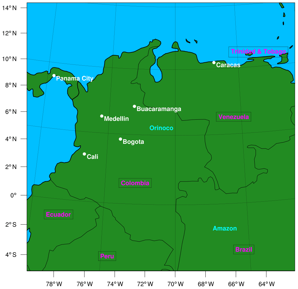
Figure 1WRF-Chem domain including countries (pink), major cities (white) and regions (blue).
Table 1WRF-Chem physical and chemical parametrization schemes.
The simulation was set up for one domain with a spatial resolution of 27 km centered at 4.89∘ N, 71.07∘ W. The entire domain consists of 100 grid points in both the north–south and the east–west direction, with 60 vertical levels – in a sigma coordinate system – up to 50 hPa. The simulation length is 1 month (also given technical constraints on conducting much longer integrations with WRF-Chem), with a spin-up time of 24 h, covering the whole month of January 2014. The selection of this study period is motivated by the fact that January is the dry season in Colombia during which the loss of remote sensing data due to presence of clouds is minimized (see Sect. 3.1.1). In addition, in Sect. 5 we show how the selected study period can be put into the context of the baseline state of air quality in Colombia using the interannual and seasonal variability in emission sources inferred from the remote sensing observations. The European Centre for Medium-Range Weather Forecasting (ECMWF) ERA-Interim product provides us with the meteorological initial and boundary conditions. The chemical initial and boundary conditions are constrained with the Copernicus Atmosphere Monitoring Service (CAMS) near-real-time data set. The boundary conditions are updated every 6 h on a spatial resolution of 0.4∘ (∼44 km) with 60 vertical model levels. For January 2014, boundary conditions of O3, NOx, CO, SO2 and CH2O are available. For tropospheric chemistry, the Carbon-Bond Mechanism version Z (CBM-Z) chemical scheme (Gery et al., 1989; Zaveri and Peters, 1999) is used here because it has been successfully implemented and tested in similar studies (Gupta and Mohan, 2015). Additional parametrization schemes used in this research are listed in Table 1.
2.2 Emission inventories
Anthropogenic emissions are described by the Emission Database for Global Atmospheric Research (EDGAR) data set for greenhouse gases (Janssens-Maenhout et al., 2019) and nonmethane volatile organic compounds (NMVOCs) (Huang et al., 2017). Emission estimates are gridded on a resolution. EDGAR emissions are monthly estimates implying constant emissions over the whole simulation. In this study we use the EDGAR data set coupled with the Hemispheric Transport of Air Pollution (HTAP; collectively EDGAR–HTAP) emission inventory updated for 2010. EDGAR–HTAP uses nationally reported emissions combined with regional scientific inventories. For this research we assumed that 95 % of the total anthropogenic emission of NOx is emitted as NO and 5 % as NO2 (Carslaw, 2005). Volatile organic compounds (VOCs) speciation is according to Archer-Nicholls et al. (2014). In densely populated urban areas, the anthropogenic emissions are dominated by vehicular emissions (Dodman, 2009). These emissions have a clear diurnal and weekly variation in contrast to emissions from the industry sector (Streets et al., 2003). Zárate et al. (2007) estimated traffic emission factors for Bogotá using in situ measurements and inverse modeling techniques. To account for this diurnal and weekly variation, we multiply the EDGAR emissions with the hourly and daily emission factors presented by Zárate et al. (2007).
The Global Fire Emissions Database version 4 (GFEDv4) data set (Randerson et al., 2015) provides us with the biomass burning emissions. GFED is available on a spatial resolution of , approximately the same size as the WRF-Chem grid cells. Biomass burning NOx emissions are assumed to be completely in the form of NO.
Natural emissions of VOCs from terrestrial ecosystems are considered in this study using the Model of Emissions of Gases and Aerosols from Nature version 2.1 (MEGAN2.1) (Guenther et al., 2012). Biogenic emissions are updated on-line using the WRF-Chem simulated surface temperature, soil moisture, leaf area index and photosynthetically active radiation. MEGAN also provides estimates of soil biogenic NO emissions.
The lightning–NOx parametrization scheme (Price and Rind, 1992), embedded in WRF-Chem, is used to account for NOx emissions by lightning. For this study we used an intracloud : cloud-to-ground (IC:CG) ratio of 2 : 1 constant over the whole domain, with a flash rate factor of 0.1. For each lightning flash (both for IC and CG strikes), it is assumed that 250 moles of NO are emitted (Miyazaki et al., 2014). It has to be noted that in an initial simulation, using standard WRF-Chem settings (flash rate factor =1.0 and 500 moles of NO per strike), resulted in a significant overestimation of the lightning emissions (see Sect. 4.1; Bradshaw et al., 2000; Miyazaki et al., 2014; Murray, 2016). The settings we used resulted in a 20-fold decrease in lighting emissions compared to standard WRF-Chem settings.
3.1 Satellite retrievals
Observational data on the distribution of NO2 are retrieved from the Ozone Monitoring Instrument (OMI) on board the National Aeronautics and Space Administration (NASA) Aura satellite (Levelt et al., 2006). OMI measures, among other pollutants, NO2 column densities (Boersma et al., 2007) with daily, global coverage. The pixel size of 24×13 km2 may be coarse for particular applications, such as assessing urban pollution, but is suitable for assessing contrasts in regional-scale air quality with apparent contrasting emission regimes. In addition, the resolution of the OMI observations is also comparable to the resolution of the anthropogenic emission inventory.
In this research we use the Quality Assurance for Essential Climate Variables (QA4ECV) NO2 data product (Boersma et al., 2018). The measured slant columns – the tilted path directly from the Sun through the atmosphere to the surface and back to the satellite – are converted to vertical columns using air mass factors (AMFs; –) by the following:
where VCD and SCD are the vertical column density and the slant column density (molecules cm−2), respectively. The AMFs define the relation between slant column and the vertical column above a pixel based on external information on, for example, surface albedo, scattering, clouds and the vertical distribution of NO2 (Boersma et al., 2011). The vertical distributions of NO2 in the QA4ECV product, which are used to calculate the AMFs, are simulated by the TM5-MP global chemistry transport model at a resolution of (Williams et al., 2017).
3.1.1 Filtering
We follow the data filtering recommendations by the QA4ECV consortium. The presence of clouds (cloud radiance fraction >0.5) led to the omission of 63 % of OMI NO2 data. Figure 2 shows the amount of OMI data per WRF-Chem grid cell after filtering the observations of January 2014. Especially above mountainous regions, where we also find the main urban areas of Bogotá and Medellín, there is a lack of available data due to the continuous presence of clouds. This limits the quality of the measurements, which increases the uncertainty in the averaged tropospheric NO2 column (Boersma et al., 2018). On average, 9 data points per grid cell are available for this specific domain in January 2014 but with a large spatial heterogeneity. Some areas have >20 data points and others only have two valid observations in this month.
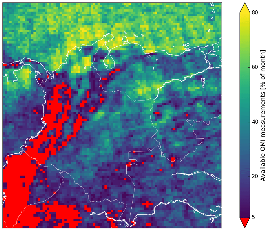
Figure 2Spatial distribution of the available OMI measurements in January 2014 after filtering was applied.
3.1.2 AMF recalculation
The AMF depends on assumptions of the state of the atmosphere and surface (e.g., surface albedo, cloud fraction and vertical distribution of NO2) at the specific moment and location of a satellite observation (Lorente et al., 2017). This vertical sensitivity is described by an averaging kernel, which describes the relationship between the true column and the estimated, or retrieved, column (Boersma et al., 2016). High-resolution models such as WRF-Chem are expected to better represent the spatial gradients in NO2 profiles compared to coarse-scale global models such as GEOS-Chem or TM5-MP. Consequently, we can expect WRF-Chem to better resolve strong enhancements in tropospheric NO2 VCDs in densely populated areas. Using grid sizes comparable to the size of such large urban areas is a major advantage of this procedure (Krotkov et al., 2017). The application of the averaging kernel is shown to reduce systematic representativeness errors for a satellite–model comparison (Boersma et al., 2016). We can recalculate the AMFs based on the a priori concentration profile xa (from the TM5-MP model), and the concentration profile in the high-resolution model, xm, in this study of WRF-Chem (Boersma et al., 2016) is as follows:
where M(xa) is the tropospheric AMF used in the retrieval, Al are the elements of the averaging kernel for each l vertical layer and M′(xm) is the recalculated AMF. In a next step, the new VCDs can be calculated by dividing the SCDs (retrieved by the satellite) with the recalculated AMFs (Eq. 1).
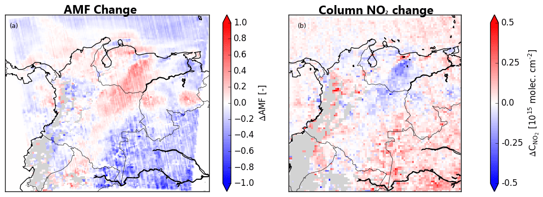
Figure 3Spatial distribution of (a) the AMF difference (recalculated minus QA4ECV standard product; ΔAMF; –) in January 2014 based on the WRF-Chem simulation and (b) the subsequent effect on the NO2 column difference (recalculated minus QA4ECV standard product; ; 1015 molecules cm−2) on the WRF-Chem grid.
Figure 3 shows the difference in AMFs and the subsequent effect on the tropospheric NO2 columns for the WRF-Chem domain. On average, we find a mean decrease in AMF of 0.05, with a standard deviation of 0.15. Regarding inferred changes in the VCD due to this recalculation of AMFs, we find a mean increase in the VCD of 0.02×10¹⁵ molecules cm−2 (∼3 % of the average VCD) and a standard deviation of 0.07×10¹⁵ molecules cm−2. Above cities (e.g., Caracas, Bogotá and Medellín), we mostly find a decrease in AMFs (Fig. 3a) and, consequently, an increase in VCD (Fig. 3b). This indicates that there is more NO2 present near the surface in WRF-Chem compared to TM5. This is consistent with our expectation that WRF-Chem better captures the processes that occur at a scale below that are not resolved by TM5, such as the localized urban emissions. Furthermore, we find increases in VCD (0.5×10¹⁵ molecules cm−2) above the Amazon region. Decreases in VCD (Fig. 3b) are found mostly across the border from Colombia to Venezuela, better known as the Orinoco region (Fig. 1). This reflects a higher abundance of NO2 higher up in the troposphere from lightning sources, which are potentially underestimated by the global TM5 model (Silvern et al., 2018), combined with less NO2 near the surface. We also find two isolated hot spots of decreases in VCDs in southern Venezuela which correlate well with the topography within the WRF-Chem domain, which is less well resolved in the coarser resolution of TM5. Despite locally significant changes in VCDs, a domain average of 0.6×10¹⁵ molecules cm−2 indicates that the difference in the NO2 a priori profiles of TM5, compared to those in WRF-Chem, does not lead to domain-wide significant changes in VCDs.
3.1.3 Comparison of OMI and WRF-Chem
In WRF-Chem we calculate the tropospheric NO2 column by integrating from the surface to the tropopause, which is determined to be approximately the 50th model level (∼90 hPa; ∼17 km). This level is determined based on the average temperature profile (from surface to 50 hPa) of the complete simulation. Furthermore, to assess the daily differences in the total NO2 columns from OMI and WRF-Chem, we need to cosample their data points. For Colombia, OMI passes around 17:00–19:00 UTC (13:00 local time – LT). Grid points with no, or only one, measurement after filtering (see Fig. 2) will be completely discarded. In this way we aim to have a reliable comparison between WRF-Chem and OMI, which enables us to determine systematic biases in the regions dominated by different emission sources.
3.2 In situ data
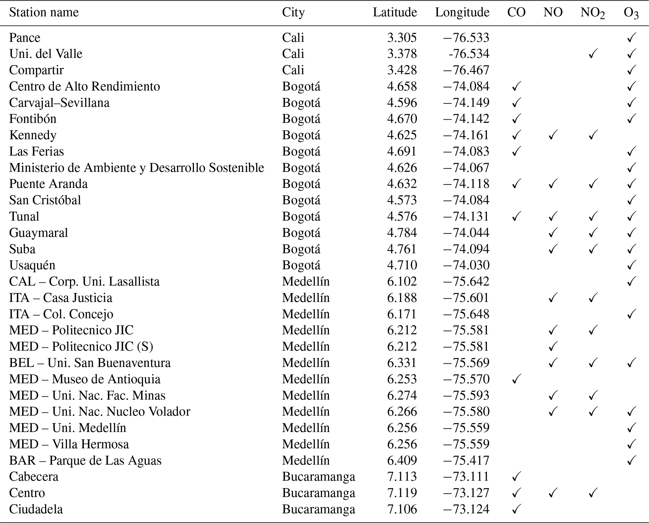
To further evaluate the model, observational data from air quality monitoring stations in Colombia are used. These include 30 stations confined to four cities in Colombia, namely Bogotá, Bucaramanga, Cali and Medellín (see Fig. 1). Observational data consist of 1-hourly averaged CO, NO, NO2 and O3 concentrations. The complete availability and locations of the station within the WRF-Chem domain can be found in Table A1. The data and information on the measurements are publicly available at http://sisaire.ideam.gov.co/ideam-sisaire-web/ (last access: 30 July 2020). In this paper we only show the results of Bogotá because the comparisons for the other cities show similar results. Even on the still coarse resolution of the current WRF-Chem simulations, we expect that the evaluation of the temporal variability in simulated and observed concentrations indicates how well the model captures some of the key drivers of atmospheric pollution.
4.1 Nitrogen emission budgets and distribution
First of all, we identify the major sources of NOx within the domain of this study. The anthropogenic and biomass burning emissions are prescribed using their inventories whereas soil NO and lightning NOx emissions are explicitly simulated in WRF-Chem. Some large cities contribute dominantly to the total NOx emissions (Fig. 4a). Total emissions are of the order of 200–1000 kg N km−2 per month for the Colombian cities. However, the largest NOx emissions, according to the EDGAR inventory, are found in and around Caracas, Venezuela. All of these emissions can be attributed to anthropogenic emissions as reflected by a ∼100 % contribution of anthropogenic emissions to the total emissions as shown in Fig. 4b. Another major source of NOx is found in the southeast of the domain, with values ranging up to 100 kg N km−2 per month. In this region, with land cover dominated by rainforest, large convective systems are present that generate thunderstorms with associated lightning NOx emissions. They appear to be the most important emissions in this region (Fig. 4b) because anthropogenic and biomass burning emissions are mostly absent (with some exceptions near rivers). Biomass burning and soil biogenic emissions seem to be the most prominent sources of NOx across the Colombian–Venezuelan border (Fig. 4b), in the Orinoco region, in our model study. This region is dominated by savanna-type grasslands which emit a relatively high amount of soil NOx but also have a high probability of catching fire. NOx emissions in these regions are up to 1 or 2 orders of magnitude smaller compared to anthropogenic emissions but, on the other hand, cover a larger area.
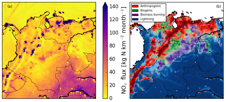
Figure 4Spatial distribution of (a) the total NOx flux (kg N km−2 per month) in January 2014 and (b) the dominant emission source per grid cell over land. In panel (b) the saturation of the color indicates the percentage of the total NOx flux coming from the dominant emission source and increasing to 100 % for the darkest colors.
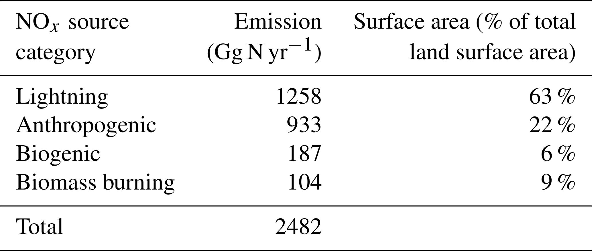
Lightning NOx emissions are the most dominant emission sources over land in 63 % of all grid cells, followed by anthropogenic (22 %), biomass burning (9 %) and biogenic (6 %) emissions (Fig. 4b). Since we use four different emission inventories, all with their own estimates and uncertainties, the distinct contrasts in the spatial distribution of emission sources will be key for determining the spatially heterogeneous biases in satellite retrievals compared to WRF-Chem. From budget calculations integrating over the whole domain, and using these January emissions to infer a NOx emission budget expressed per year (see Table 2), we also find that lightning NOx is the largest source in absolute terms, followed by anthropogenic, biogenic and biomass burning, respectively.
Table 2Total NOx emissions in the WRF-Chem domain per source category using January 2014 emissions to infer yearly total NOx emissions (Gg N yr−1). The percentage of surface area over land where the emission source is dominant is also indicated.
4.2 WRF-Chem and OMI comparison
To assess whether WRF-Chem is able to reproduce filtered and recalculated NO2 VCDs satisfactorily, we checked for the spatial and frequency distributions for both WRF-Chem and OMI (see Fig. 5). For WRF-Chem we found a wide range of column densities (Fig. 5a). We found very low VCDs ( molecules cm−2) over the Caribbean Sea and across the eastern border of Colombia into Venezuela. High VCDs in WRF-Chem are simulated above the major Colombian cities and in the northeastern part of the domain ( molecules cm−2), while the highest VCDs are simulated above the city of Caracas with values up to 8×10¹⁵ molecules cm−2. Similar to WRF-Chem, we found the lowest VCDs over the Caribbean Sea in OMI (Fig. 5b). Also, we found the highest VCDs above major cities – most pronounced for Caracas and Medellín – but the magnitude of the OMI-observed VCD ( molecules cm−2) is much smaller compared to WRF-Chem. In OMI we find low VCDs above the Amazon rainforest.
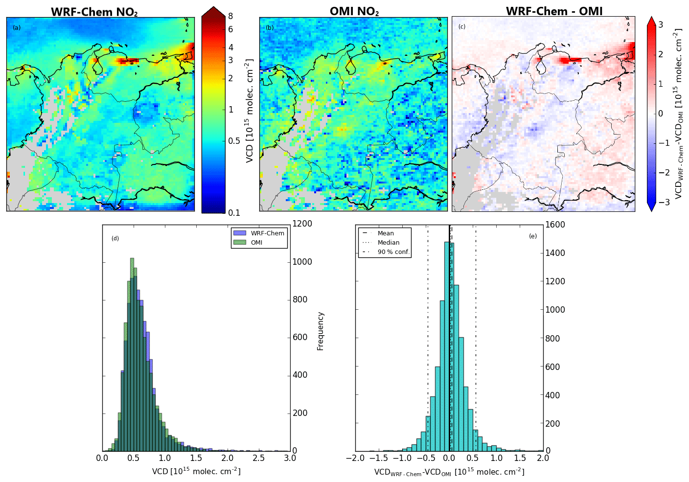
Figure 5Spatial distribution of averaged cosampled NO2 vertical column densities (VCDs; 1015 molecules cm−2) for (a) WRF-Chem, (b) OMI recalculated retrievals and (c) the absolute difference (WRF-Chem minus OMI) between the two and (d) the frequency distribution of both WRF-Chem and OMI over the whole domain and (e) the distribution of the absolute difference between the two per grid point, including mean (broken line), median (dotted line) and 90 % confidence interval (broken and dotted line).
The large WRF-Chem VCDs ( molecules cm−2) we find in the northeastern part of the domain (Fig. 5c) seem to mostly reflect the role of the imposed CAMS boundary conditions. High mixing ratios of NO2 are found in the lowest CAMS model layers advected into the WRF-Chem domain by the prevailing easterlies. High VCDs are not seen in the OMI retrievals where we only find a small plume coming from Trinidad and Tobago that is transported westward. The model's overestimation of the VCD above Caracas might be due to an overestimation of anthropogenic emissions, but this is not supported by a systematic major overestimation above cities (for example, we find no overestimation above Panama City or Bucaramanga). However, the EDGAR emission inventories are based on the year of 2010, when the Venezuelan economy was still at its highest (Wang and Li, 2016). After 2010, the Venezuelan economy and oil production declined strongly (Wang and Li, 2016) and therefore emissions of pollutants have also likely decreased substantially. Lastly, we find a systematic overestimation in the WRF-Chem simulated VCD above the Amazon rainforest. Even though the model overestimation is small in absolute terms ( molecules cm−2), it is quite substantial relative to the background mixing ratios. In this region, soil NOx release is small, anthropogenic activities are hardly present and there are no known sources of biomass burning during January 2014. Also the role of advection from outside the model domain by the prevailing easterly winds seems to be limited as indicated by lower VCDs at the easternmost grid cells. Consequently, overestimation in the simulated VCDs is most likely due to the simulated major influence of lightning NOx emissions in this region (Fig. 4b), even though they have already been significantly reduced relative to the standard settings (see Sect. 2.2). However, we have to take into account that the OMI retrievals used for this comparison are near the detection limit and reflect those conditions when cloud formation, and therefore lightning production is less active, resulting in very low VCDs. In contrast, the cosampled WRF-Chem columns might reflect simulated cloud cover resulting in production of NO by lightning. Nonetheless, the question of whether lightning production was actually present or if it could not be picked up by OMI, which is less sensitive to the presence of NO2 below the clouds, remains unanswered.
Remarkably, we find a region with systematic underestimations ranging from the center of Colombia to the northeastern border with Venezuela (the Orinoco region). In this region, there is no presence of major cities, and lightning NOx emissions are small. The discrepancy we find might be due to missing agricultural or biomass burning emissions. Localized enhancements observed in OMI ( molecules cm−2) might also be caused by biomass burning emissions since enhanced soil NOx is expected to result in a more homogeneous enhancement of VCDs over a larger area with smaller intensities. We find that this intensity of biomass burning is not picked up by the WRF-Chem simulation using the GFED biomass burning inventory.
Figure 5d shows, for both WRF-Chem and OMI, the frequency distribution in the NO2 VCD. We find that both model-simulated and observed VCDs show similar distributions, peaking at approximately the same VCD. However, WRF-Chem shows more outliers, especially regarding the simulation of high NO2 VCDs. The 90 % confidence interval of the WRF-Chem simulated VCDs is molecules cm−2, while for OMI the 90 % confidence interval is molecules cm−2, with medians of 0.59×10¹⁵ and 0.56×10¹⁵ molecules cm−2, respectively.
We find the median and mean of the absolute overestimation by WRF-Chem to be 0.02×10¹⁵ and 0.09×10¹⁵ molecules cm−2, respectively (Fig. 5e). The 90 % confidence interval equals molecules cm−2. The distribution is approximately Gaussian, with a standard deviation of 0.53×10¹⁵ molecules cm−2 but somewhat left-skewed indicating an overestimation by WRF-Chem. This confirms the finding that WRF-Chem is able to produce on average good estimations for vertical NO2 columns above Colombia. However, over- and underestimations can be significant, e.g., larger than the ∼10 % uncertainty in monthly averaged OMI VCDs over polluted regions (Boersma et al., 2018) due to numerous factors in both the model setup and the characteristics of the retrievals.
4.3 Surface-mixing ratios
Figure 6 shows the model-simulated and observed temporal evolution in NOx and O3 over the whole simulation period. WRF-Chem represents the lower limit (generally midday) of observed NOx mixing ratios but is unable to simulate the observed maxima (generally morning rush hour) up to 200 ppb for particular events. Regarding O3, WRF-Chem resembles the upper limit of observed mixing ratios (∼40 ppb) during daytime but is unable to reproduce the observed low (<5 ppb) nighttime mixing ratios.
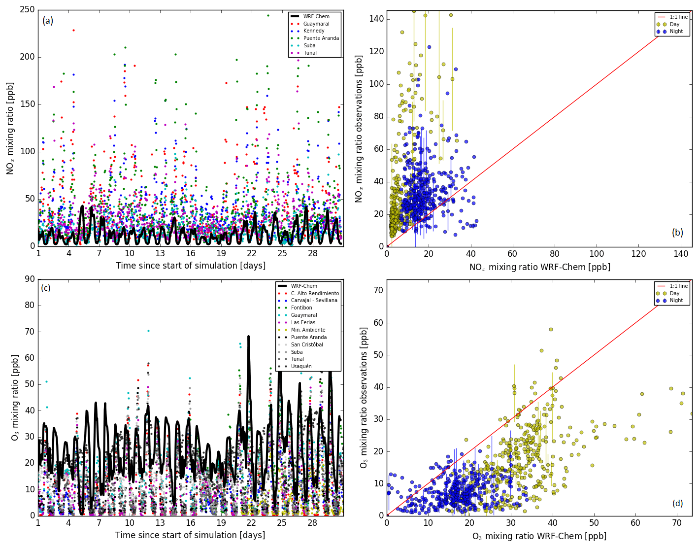
Figure 6Temporal evolution of (a) NOx and (c) O3 mixing ratios (ppb) in Bogotá for WRF-Chem (black solid line) and all available observational stations (colored points). Scatterplots of the WRF-Chem output compared with averaged (b) NOx and (d) O3 mixing ratios (ppb) from the stations are split into day (yellow) and night (blue). The error bars indicate the standard deviation of the observational data from randomly sampled points (not all standard deviations are shown for visual purposes).
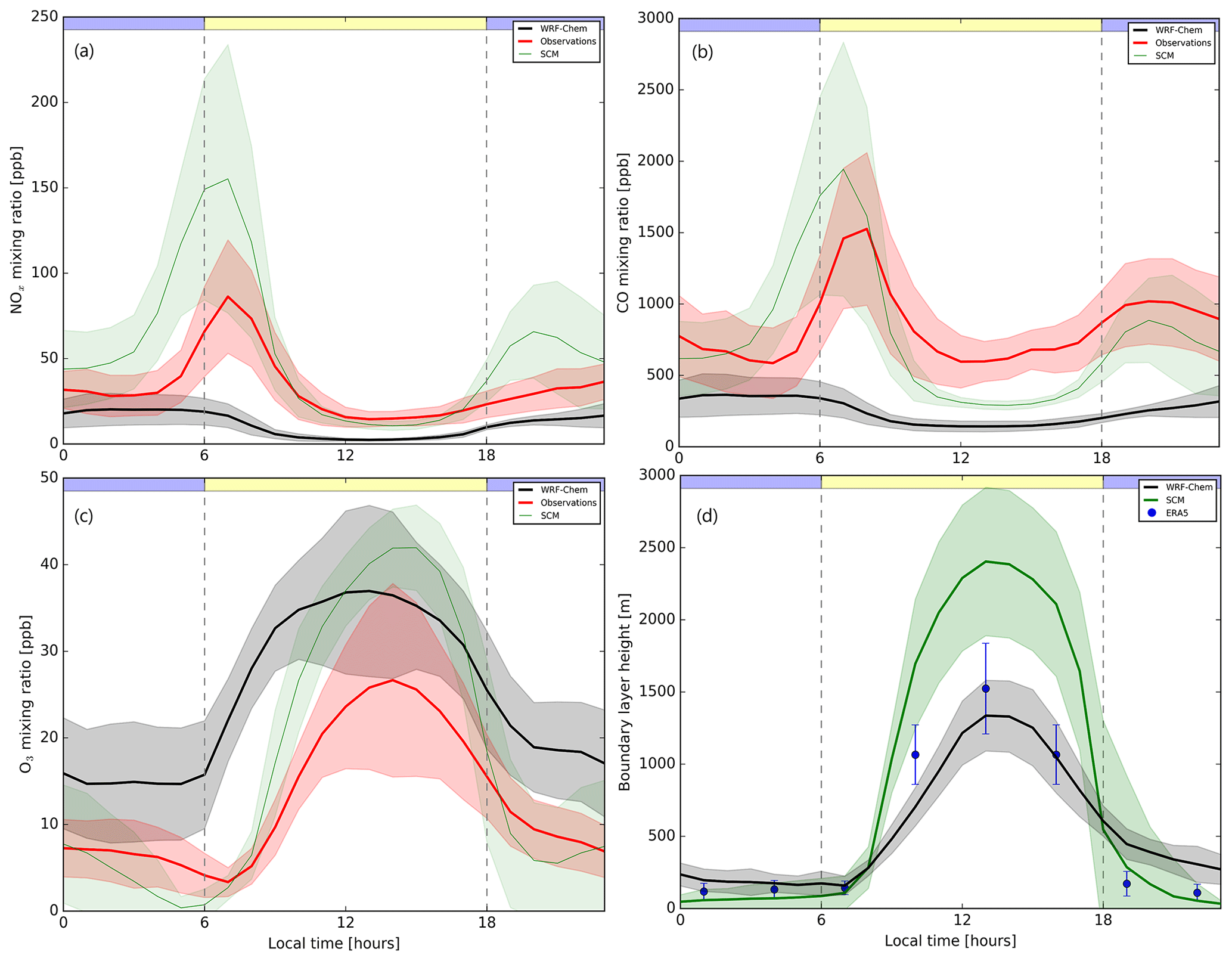
Figure 7Averaged diurnal cycle of (a) NOx, (b) CO and (c) O3 mixing ratios (ppb) and (d) boundary layer height (m) in Bogotá for WRF-Chem (black solid line), averaged observational data (red solid line), SCM (green solid line) and ERA5 reanalysis data (blue dots). The black, red and green shadings and blue error bars indicate the 30 d standard deviation of WRF-Chem, observations, SCM and ERA5, respectively. The vertical lines and blue (night) and yellow (day) shading indicate daytime and nighttime.
We retrieve January's averaged diurnal cycles in NOx, CO and O3 surface mixing ratios (Fig. 7a–c) by removing the significant spread in the observed surface mixing ratios and by averaging the day-to-day variation in both the model and observations. Regarding simulated NOx, the average nocturnal mixing ratios are 20 ppb, with some day-to-day variation (standard deviation =10 ppb), and a minimum of 2 ppb during daytime but with less day-to-day variation (Fig. 7a). The observations reach peak mixing ratios around 07:00 LT, during which vehicular emissions during rush hour are mixed in a shallow boundary layer that increases NOx mixing ratios to 85 ppb on average. After rush hour, mixing ratios decrease due to decreasing emissions, increasing boundary layer height and decreasing NOx lifetime. It is interesting to note that there does not seem to be a clear signal for the evening rush hour in the NOx measurements and simulation.
The averaged diurnal cycle of CO in WRF-Chem shows a similar pattern to that of NOx (Fig. 7b). WRF-Chem shows daytime mixing ratios of ∼150 ppb (well above the rural background-mixing ratios of 100 ppb) and ∼350 ppb during nighttime, while the surface measurements show a significantly larger variation. Averaged surface measurements during rush hour exceed CO mixing ratios of 1500 ppb. Some measurement stations even report mixing ratios above 3000 ppb. Even though nighttime emissions are mixed over a smaller boundary layer, we find that WRF-Chem underestimates surface mixing ratios of CO by a factor of 4 during rush hour and by a factor of 2 for nighttime conditions. These ratios are similar to the NOx ratios in Fig. 7a. Since CO has a relatively long lifetime compared to that of NOx, we argue that observed differences regarding simulated and observed CO mixing ratios reflect issues regarding the representativity of the WRF-Chem grid simulated pollutant levels, including the representation of emissions and online-simulated meteorological conditions relative to the footprint of the surface observations.
We find that for WRF-Chem most of the NOx is present as NO2, with NO mixing ratios being very close to 0 ppb (not shown here). In contrast, the observations show that most of the NOx is present as NO. For WRF-Chem we find a [NO]∕[NO2] ratio of ∼0.32 (±0.13) during the daytime and ∼ 0.07 (±0.04) during nighttime, while for the surface measurements these ratios are ∼1.11 (±0.40) and ∼0.89 (±0.38), respectively. The observations that show that a high [NO]∕[NO2] ratio might be indicative of a location close to local sources, e.g., roads. The abundant fresh NO emissions at these locations quickly react with O3 to form NO2. The surplus NO, however, pushes the [NO]∕[NO2] ratio up. Indeed, a simulated underestimation by WRF-Chem of 10 ppb NO during the nighttime is consistent with a simulated overestimation of 10 ppb O3 (Fig. 7c). We also find that in WRF-Chem, the formation of O3 immediately starts at 06:00 LT (sunrise), while for the observations we find the lowest mixing ratios at 07:00 LT due to the extra NO titration caused by the rush hour. Nonetheless, it seems that chemical production and destruction rates of O3 and other processes contributing to the overall magnitude and diurnal cycle in O3, e.g., entrainment and deposition, are well captured by WRF-Chem considering the similar shape and amplitude of the diurnal cycle.
To test the hypothesis that the model–data mismatch over Bogotá is caused by too coarse a model resolution or a misrepresentation of emissions, we conducted additional experiments with a single-column chemistry–meteorological model (SCM), also being previously applied for an analysis of observations of the plume of pollution downwind of the city of Manaus (Brazil; Kuhn et al., 2010). The SCM simulates, similar to WRF-Chem, atmospheric chemistry processes online, including anthropogenic and natural emissions, gas-phase chemistry, wet and dry deposition, and turbulent and convective tracer transport as a function of meteorological and hydrological drivers, surface cover and land-use properties (Ganzeveld et al., 2002b, 2008). For these urban area simulations with the SCM we have modified the surface cover properties by prescribing surface roughness at 1 m, assuming a reduced vegetation fraction of 0.6 using a city area albedo of 0.18, and nudged the SCM meteorology with wind speed, moisture and temperature profiles from the WRF-Chem simulation. The SCM is also nudged with long-lived tracers such as O3, NOx and CO above the boundary layer using WRF-Chem mixing ratios. Finally, we also used the same emissions, including diurnal cycle, as in the WRF-Chem simulation.
Using these settings in the SCM results in the simulated January average diurnal cycles in NOx and CO, which is quite different from WRF-Chem but in better agreement with the observations in terms of 30 d average diurnal cycles, maximum early morning peak and daytime minimum mixing ratios of NOx and CO (Fig. 7a–b). The skewed O3 diurnal cycle (Fig. 7c) is also better reproduced compared to WRF-Chem although the overestimation of the maximum afternoon mixing ratios is larger. Figure 7d shows a comparison of the SCM, WRF-Chem simulated and the ERA5 reanalysis boundary layer height for the grid point resembling the location of Bogotá. The SCM shows a substantially deeper daytime maximum boundary layer with more day-to-day variation compared to WRF-Chem and ERA5 reanalysis data. The SCM also simulates a relatively fast afternoon transition to suppressed nocturnal mixing conditions reflected by a nocturnal inversion layer, which agrees well with the ERA5 boundary layer height being shallower than that simulated by WRF-Chem. Interestingly, the SCM simulation results in a better representation of the observed diurnal cycle of urban pollutant mixing ratios, especially regarding the observed early morning maximum CO and NOx and minimum O3 concentrations, without requiring the hypothesized enhancement in emissions. This stresses that, besides the application of higher-resolution emission inventories and model experiments, the diurnal cycle in boundary layer dynamics (and advection) should be critically evaluated in models such as WRF-Chem which, however, would then also require urban boundary layer structure measurements.
The integration of global emission inventories in a highly resolved coupled meteorology–air quality model (WRF-Chem), with roughly the same spatial scale, allowed us to assess the state of – and contribution by – different sources to the air quality in Colombia and neighboring countries as diagnosed with a focus on NOx. We identified four major sources of NOx in Colombia which were implemented in WRF-Chem partly through emission inventories (anthropogenic and biomass burning) and partly through emission models (soil NO and lightning). Using January's emissions to infer a NOx emission budget expressed per year, we found that lightning NOx emissions are the main source for the domain applied in this study, with 1258 Gg N yr−1. These are followed by, respectively, anthropogenic (933 Gg N yr−1), soil biogenic (187 Gg N yr−1) and biomass burning (104 Gg N yr−1) emissions. Figure 8 shows the averaged VCDs over the regions dominated by one of the four emissions classes (Fig. 4b). Figure 8a shows the yearly trends in OMI NO2 VCDs. The domain averaged anthropogenic- or lightning-dominated regions seem to have relatively low interannual variability. The biogenic- and biomass-burning-dominated regions show the most interannual variability which also seem to correlate with the El Niño years (https://origin.cpc.ncep.noaa.gov/products/analysis_monitoring/ensostuff/ONI_v5.php, last access: 30 July 2020), with the exception of 2015. Colombia is relatively warm and dry during the El Niño years (Córdoba-Machado et al., 2015). Figure 8a indicates that biogenic- and biomass-burning emissions might have increased during El Niño years as reflected by January's higher monthly mean VCDs above those regions. To further put the findings of the combined WRF-Chem and OMI VCDs for January 2014 in context, Fig. 8b shows the seasonal variability in OMI NO2 VCDs. We find that biogenic, biomass burning and anthropogenic emissions show a maximum at the end of the dry season (March). For biogenic and biomass burning this is most likely caused by increased emissions, while for the domain dominated by anthropogenic emissions this is most likely caused by advection of NOx emitted by biogenic or biomass burning sources located upwind. For lightning, NO2 VCDs we find a maximum in August or September. We find that this is caused by an increase in NO2 VCDs in the southeastern part of the domain (the Amazon region), not shown here. The large standard deviation in the biomass burning NO2 VCDs again indicates the large interannual variability. Based on this further analysis of the long-term trends in OMI NO2 VCDs, we argue that the 2014 simulation and remote sensing data analysis is a reasonably good approximation of the baseline state of air quality in Colombia, at least regarding NOx. However, we have to take into account the interannual and seasonal variability in NOx emissions in interpreting the OMI data and WRF-Chem results.
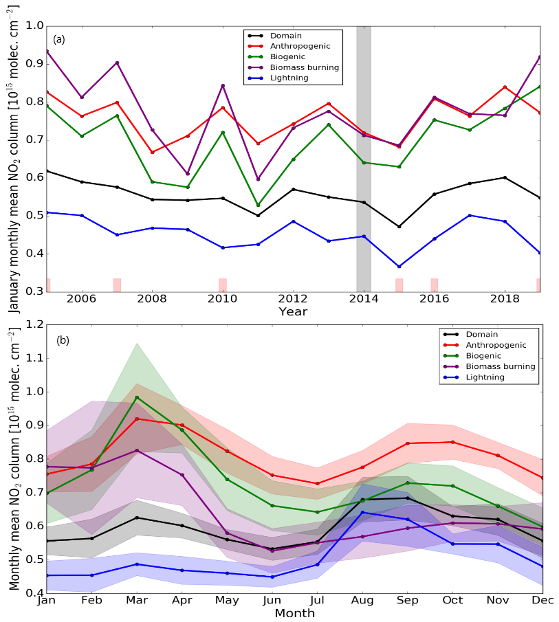
Figure 8(a) January's monthly averaged NO2 vertical column densities (1015 molecules cm−2) retrieved from OMI for 2005–2019 for the whole domain (black), regions with dominating anthropogenic (red), biogenic (green), biomass burning (yellow) and lightning (blue) emissions. The gray vertical bar highlights the WRF-Chem simulated year 2014. The red bars indicate El Niño years (2005, 2007, 2010, 2015, 2016 and 2019). (b) Monthly averaged OMI NO2 vertical column densities (1015 molecules cm−2) for 2005–2019. The shadings indicate ±1 standard deviation.
The top-down validation approach, using satellite retrievals, is a valuable tool for evaluating air quality in remote regions (Bailey et al., 2010; Webley et al., 2012) with a missing network of air quality monitoring in both urban and rural sites. The daily global coverage and retrievals of NO2 by OMI (Levelt et al., 2006) were used to assess the quality of all emission inventories over the whole domain. However, 63 % of the data are lost for this specific model setup, mainly due to the continuous presence of clouds. Thus, longer simulation times have to be considered in the tropics compared to midlatitudes. The vertical distribution of NOx within a modeling environment is key for identifying discrepancies in a top-down validation approach using satellite retrievals. It has to be recognized that the satellite sensitivity is reduced towards the surface (Boersma et al., 2016), inducing enhanced differences between observed and modeled profiles. However, this can be overcome by replacing a priori TM5 profiles with those from the applied model (Boersma et al., 2016).
In contrast to the bottom-up validation approach, where WRF-Chem showed a significant underestimation of NOx compared to the in situ measurements, we found that WRF-Chem does not systematically underestimate urban VCDs. This suggests that the problem is indeed bound to the representativeness of WRF-Chem with respect to subgrid-scale emissions and other processes and not so much to the magnitude of anthropogenic emissions. The underestimation by WRF-Chem in the Orinoco region, where biogenic and biomass burning emissions make up a great part of the emission budget, indicates an underestimation of biomass burning emissions. Biogenic emissions are expected to show a more homogeneous distribution over a larger area with less pronounced peak emissions.. Therefore, they are also not expected to explain VCDs over the 2×10¹⁵ molecules cm−2 we found in OMI retrievals. This connects to the findings of Grajales and Baquero-Bernal (2014), who concluded that high VCDs in this region are most likely related to biomass burning, which is apparently underestimated by the emission inventory we applied in this study. Soil NO emissions might be underestimated due to the missing anthropogenic term (fertilizer and manure application; Visser et al., 2019). However, enhanced soil NO emissions due to the use of fertilizer is estimated to only contribute ∼1.3 % to the total soil NO flux in the global chemistry–climate model, namely ECHAM/MESSy Atmospheric Chemistry (EMAC) model, (∼2.8∘) for this domain (Ganzeveld et al., 2010). Furthermore, the simulated soil biogenic NO flux (187 Gg N yr−1) from MEGAN is in the range between the total soil NO flux (230 Gg N yr−1) and the NO flux at the top of the canopy (105 Gg N yr−1) estimated by EMAC.
We find a large area with overestimations of modeled VCDs in the region dominated by lightning NOx emissions. These findings are in contrast with Grajales and Baquero-Bernal (2014), who found in their study with the GEOS-Chem modeling system that, in remote regions without biomass burning, there is an underestimation of modeled VCDs. Our study indicates that lightning NOx emissions are a major source of NOx, which might explain the discrepancy in the study by Grajales and Baquero-Bernal (2014) in which this source was not considered. Also, the use of WRF-Chem, with a spatial resolution approximately the same size as the OMI observations, can be advantageous over coarser models such as GEOS-Chem used by Grajales and Baquero-Bernal (2014). Further attention is required, not only regarding the lightning NOx parametrization scheme but also regarding the model representation of convection and clouds, either in follow-up studies on atmospheric NOx over Colombia or other regions where lightning is a dominant source of NOx. This study does not aim to provide comprehensive estimates of any of the emission sources using OMI data. Rather, we show the potential use of satellite data in a region with a limited air quality monitoring network to determine the regional-scale air quality and NOx source regions. The use of cloud-covered OMI observations to get a more comprehensive estimate of lightning NOx emissions (Beirle et al., 2010; Pickering et al., 2016) would make a very interesting follow-up study.
The air quality monitoring network in Colombia is limited to four major cities. This implies that the validation is limited to urban areas where anthropogenic emissions are the dominant source of pollution. A comparison with in situ data showed that WRF-Chem systematically underestimates urban surface mixing ratios of NOx and CO. The surface observations showed a clear signal of morning rush hour emissions with average observed NOx mixing ratios up to 90 ppb and single observations not rarely exceeding 150 ppb. Similar to González et al. (2018), who focused on O3 dynamics in Manizales (a medium-sized Andean city), we find an overestimation of O3 by WRF-Chem both during the nighttime and daytime. For Manizales, NOx measurements were not available (González et al., 2018) and were proposed to explain most of the inferred discrepancies between the observed and simulated O3 mixing ratios. In this study we found that the underestimation of NO by ∼10 ppb translates to an overestimation of ∼10 ppb O3. Even though O3 production and destruction seems to be well captured by WRF-Chem, local emission inventories, including a more detailed spatial resolution around cities, can provide the extra detail needed for a subgrid-scale analysis of the interactions between local-scale emissions, chemistry, mixing and the resulting pollutant concentrations (González et al., 2018). However, as shown in Sect. 4.3, a nested domain with local, high-resolution emission inventories might not be the main solution for properly simulating urban pollutant concentrations. EDGAR emissions, as included in WRF-Chem but then applied in the SCM simulations, resulted in averaged diurnal cycles of O3, CO and NOx that agreed reasonably well with the observed diurnal cycles. The main difference was that the SCM simulations were especially showing differences regarding the nocturnal inversion compared to WRF-Chem.
One of the regions that is currently undergoing major land-use changes is the Orinoco. Its traditional agriculture and extensive grazing is shifting rapidly towards a more intensified production of food, biofuels and rubber (Lavelle et al., 2014). Especially oil palm, which is one of the world's most rapidly expanding crops (Fitzherbert et al., 2008), is becoming more and more dominant in the Orinoco region (Vargas et al., 2015). Also, urbanization in Colombia is continuously increasing (Samad et al., 2012). Ongoing and anticipated future transformation of both rural and urban areas, in combination with expected increases in temperature and changes in the hydrological cycle, imply changes in emission budgets that will affect air quality in the future. Further consistent coupling of land-use classes with emission representations may provide valuable information of the future-predicted air quality in Colombia. This includes anthropogenic, biomass burning, biogenic and lightning emissions, which apparently all having a generally dominant role in atmospheric NOx cycling in different regions of Colombia.
This study presented an analysis of the baseline state of air quality in Colombia, focusing on NOx as the main metric. Using a highly resolved coupled meteorology–air quality model (WRF-Chem), with roughly the same scale as both global emission inventories and satellite retrievals (OMI), allowed us to identify sources of pollution and the baseline state of air quality in Colombia. The main findings illustrate that, within the modeling domain, lightning (1258 Gg N yr−1), anthropogenic (933 Gg N yr−1), soil biogenic (187 Gg N yr−1) and biomass burning emissions (104 Gg N yr−1) all contribute to the total nitrogen emission budget. Especially the spatial distribution, clearly identifying regions with different dominating NOx sources, shows the importance of providing good estimates of each individual NOx source. The top-down validation approach, using OMI retrievals, indicated a mean bias of NO2 vertical column densities (VCDs) of 0.02×10¹⁵ molecules cm−2, which is <5 % of the mean column, with a 90 % confidence interval of molecules cm−2. The VCDs in the Amazon region are overestimated in WRF-Chem, even after an already strongly reduced production efficiency, with respect to the low cloud-free VCDs in OMI which are operating near the detection limit. This is a region where lightning NOx emissions are the only significant source of NO2. Additionally, the comparison indicates that GFED biomass burning emissions are potentially underestimated for January 2014 since OMI showed some strong enhancements in NO2 that are not being reproduced by WRF-Chem. The biomass burning emission inventory shows some presence of wildfires in that region, but the model only produces estimates of VCDs of molecules cm−2, compared to OMI VCDs of up to 2×10¹⁵ molecules cm−2, in regions where it is known to have significant biomass burning sources. Air mass factors (AMFs) were recalculated based on the vertical distribution of NO2 within WRF-Chem with respect to the coarse () a priori profiles for a more consistent model–satellite comparison. An analysis of the past 1.5 decades of OMI NO2 VCD data showed that the selected simulation period is representative of the baseline state of air quality in Colombia but that interannual and seasonal variability have to be taken into account when interpreting the OMI data and WRF-Chem simulations. The interannual variability in NO2 columns over the different source regions can be attributed to specific events such as the El Niño–Southern Oscillation (ENSO), whereas the seasonal variability shows a strong enhancement of NO2 VCDs above biogenic and biomass burning regions at the end of the dry season.
The bottom-up validation approach, using air quality monitoring stations in urban areas, showed that WRF-Chem, at the relative coarse resolution, does not reproduce these observations given the role of large heterogeneity in the emissions and other processes that determine pollution levels. The application of the anthropogenic EDGAR emission inventory ( resolution) in WRF-Chem resulted in a simulated underestimation of NOx and CO mixing ratios with respect to the local urban surface measurements. However, WRF-Chem was able to simulate the diurnal amplitude in O3 reasonably well for all urban locations. It seems that the underestimation of ∼10 ppb O3 during both the day- and nighttime can be attributed to the underestimation of NO by ∼10 ppb. Additional sensitivity simulations were performed with a single-column model (SCM), which showed an especially shallower nocturnal inversion layer compared to that simulated in WRF-Chem. This resulted in a better representation of the observed diurnal cycle of the urban pollutant mixing ratio without the hypothesized enhancement in emissions. This indicated that, besides the use of local emissions inventories in highly resolved modeling systems, it is also essential to carefully assess the role of boundary layer dynamics, in particular the representation of nocturnal mixing conditions, in evaluating simulations of pollutant concentrations.
In this study we presented a concise method, integrating both in situ and remote sensing observations with a mesoscale modeling system, to arrive at a quantification of air quality in regions with a limited measurement network to cover the large spatial heterogeneity in air pollution source distribution. Results obtained in this study provide insight into the baseline state of air quality in Colombia, which is essential for applying the presented combined modeling and measurement approach to also assess how air quality will further change due to future industrialization and land-use changes.
Table A1Available air quality monitoring stations including city, location and measured compounds. Note that JIC – Jaime Isaza Cadavid and S – semiautomatic equipment.
OMI data, in situ data and WRF-Chem output and scripts for recalculating the tropospheric AMFs are available upon request.
JGMB and LNG designed the experiment. JGMB performed the WRF-Chem simulations, and LNG performed the single-column model simulations. JGMB performed the analysis and wrote the paper, with contributions from all coauthors.
The authors declare that they have no conflict of interest.
We greatly appreciate the two anonymous reviewers for their critical and constructive comments. Their effort has contributed to major improvements in this paper. Furthermore, the authors acknowledge Oscar Julian Guerrero Molina from the Instituto de Hidrología, Meteorología y Estudios Ambientales (IDEAM) for providing us with air quality monitoring data. We acknowledge WRF-Chem developers and emission inventory (EDGAR, MEGAN and GFED) developers. We also acknowledge the QA4ECV consortium for making OMI NO2 data publicly available. We are thankful for Folkert Boersma's input to the OMI analysis.
This paper was edited by Jason West and reviewed by two anonymous referees.
Archer-Nicholls, S., Lowe, D., Utembe, S., Allan, J., Zaveri, R. A., Fast, J. D., Hodnebrog, Ø., Denier van der Gon, H., and McFiggans, G.: Gaseous chemistry and aerosol mechanism developments for version 3.5.1 of the online regional model, WRF-Chem, Geosci. Model Dev., 7, 2557–2579, https://doi.org/10.5194/gmd-7-2557-2014, 2014. a
Ashmore, M. R. and Marshall, F.: Ozone impacts on agriculture: an issue of global concern, in: Adv. Bot. Res., 29, 31–52, 1998. a
Bailey, J. E., Dean, K. G., Dehn, J., Webley, P. W., Power, J., Coombs, M., and Freymueller, J.: Integrated satellite observations of the 2006 eruption of Augustine Volcano, U.S. Geol. Surv. Prof. Pap., 1769, 481–506, 2010. a, b
Baklanov, A., Schlünzen, K., Suppan, P., Baldasano, J., Brunner, D., Aksoyoglu, S., Carmichael, G., Douros, J., Flemming, J., Forkel, R., Galmarini, S., Gauss, M., Grell, G., Hirtl, M., Joffre, S., Jorba, O., Kaas, E., Kaasik, M., Kallos, G., Kong, X., Korsholm, U., Kurganskiy, A., Kushta, J., Lohmann, U., Mahura, A., Manders-Groot, A., Maurizi, A., Moussiopoulos, N., Rao, S. T., Savage, N., Seigneur, C., Sokhi, R. S., Solazzo, E., Solomos, S., Sørensen, B., Tsegas, G., Vignati, E., Vogel, B., and Zhang, Y.: Online coupled regional meteorology chemistry models in Europe: current status and prospects, Atmos. Chem. Phys., 14, 317–398, https://doi.org/10.5194/acp-14-317-2014, 2014. a
Bauer, P., Thorpe, A., and Brunet, G.: The quiet revolution of numerical weather prediction, Nature, 525, 47–55, 2015. a
Beirle, S., Huntrieser, H., and Wagner, T.: Direct satellite observation of lightning-produced NOx, Atmos. Chem. Phys., 10, 10965–10986, https://doi.org/10.5194/acp-10-10965-2010, 2010. a
Boersma, K. F., Eskes, H. J., Veefkind, J. P., Brinksma, E. J., van der A, R. J., Sneep, M., van den Oord, G. H. J., Levelt, P. F., Stammes, P., Gleason, J. F., and Bucsela, E. J.: Near-real time retrieval of tropospheric NO2 from OMI, Atmos. Chem. Phys., 7, 2103–2118, https://doi.org/10.5194/acp-7-2103-2007, 2007. a
Boersma, K. F., Eskes, H. J., Dirksen, R. J., van der A, R. J., Veefkind, J. P., Stammes, P., Huijnen, V., Kleipool, Q. L., Sneep, M., Claas, J., Leitão, J., Richter, A., Zhou, Y., and Brunner, D.: An improved tropospheric NO2 column retrieval algorithm for the Ozone Monitoring Instrument, Atmos. Meas. Tech., 4, 1905–1928, https://doi.org/10.5194/amt-4-1905-2011, 2011. a
Boersma, K. F., Vinken, G. C. M., and Eskes, H. J.: Representativeness errors in comparing chemistry transport and chemistry climate models with satellite UV–Vis tropospheric column retrievals, Geosci. Model Dev., 9, 875–898, https://doi.org/10.5194/gmd-9-875-2016, 2016. a, b, c, d, e
Boersma, K. F., Eskes, H. J., Richter, A., De Smedt, I., Lorente, A., Beirle, S., van Geffen, J. H. G. M., Zara, M., Peters, E., Van Roozendael, M., Wagner, T., Maasakkers, J. D., van der A, R. J., Nightingale, J., De Rudder, A., Irie, H., Pinardi, G., Lambert, J.-C., and Compernolle, S. C.: Improving algorithms and uncertainty estimates for satellite NO2 retrievals: results from the quality assurance for the essential climate variables (QA4ECV) project, Atmos. Meas. Tech., 11, 6651–6678, https://doi.org/10.5194/amt-11-6651-2018, 2018. a, b, c
Bond, D. W., Steiger, S., Zhang, R., Tie, X., and Orville, R. E.: The importance of NOx production by lightning in the tropics, Atmos. Environ., 36, 1509–1519, 2002. a
Bradshaw, J., Davis, D., Grodzinsky, G., Smyth, S., Newell, R., Sandholm, S., and Liu, S.: Observed distributions of nitrogen oxides in the remote free troposphere from the NASA global tropospheric experiment programs, Rev. Geophys., 38, 61–116, 2000. a, b
Carslaw, D. C.: Evidence of an increasing NO2∕NOx emissions ratio from road traffic emissions, Atmos. Environ., 39, 4793–4802, 2005. a
Chen, F. and Dudhia, J.: Coupling an advanced land surface–hydrology model with the Penn State–NCAR MM5 modeling system. Part I: model implementation and sensitivity, Mon. Weather Rev., 129, 569–585, 2001. a
Córdoba-Machado, S., Palomino-Lemus, R., Gámiz-Fortis, S. R., Castro-Díez, Y., and Esteban-Parra, M. J.: Influence of tropical Pacific SST on seasonal precipitation in Colombia: prediction using El Niño and El Niño Modoki, Clim. Dynam., 44, 1293–1310, 2015. a
Dodman, D.: Blaming cities for climate change? An analysis of urban greenhouse gas emissions inventories, Environ. Urban., 21, 185–201, 2009. a
Dudhia, J.: Numerical study of convection observed during the winter monsoon experiment using a mesoscale two-dimensional model, J. Atmos. Sci., 46, 3077–3107, 1989. a
Fitzherbert, E. B., Struebig, M. J., Morel, A., Danielsen, F., Brühl, C. A., Donald, P. F., and Phalan, B.: How will oil palm expansion affect biodiversity?, Trends Ecol. Evol., 23, 538–545, 2008. a
Ganzeveld, L., Lelieveld, J., Dentener, F., Krol, M., Bouwman, A., and Roelofs, G.-J.: Global soil-biogenic NOx emissions and the role of canopy processes, J. Geophys. Res.-Atmos., 107, ACH 9-1–ACH 9-17, https://doi.org/10.1029/2001JD001289, 2002a. a
Ganzeveld, L., Lelieveld, J., Dentener, F., Krol, M., and Roelofs, G.-J.: Atmosphere–biosphere trace gas exchanges simulated with a single-column model, J. Geophys. Res.-Atmos., 107, ACH 8-1–ACH 8-21, https://doi.org/10.1029/2001JD000684, 2002b. a
Ganzeveld, L., Eerdekens, G., Feig, G., Fischer, H., Harder, H., Königstedt, R., Kubistin, D., Martinez, M., Meixner, F. X., Scheeren, H. A., Sinha, V., Taraborrelli, D., Williams, J., Vilà-Guerau de Arellano, J., and Lelieveld, J.: Surface and boundary layer exchanges of volatile organic compounds, nitrogen oxides and ozone during the GABRIEL campaign, Atmos. Chem. Phys., 8, 6223–6243, https://doi.org/10.5194/acp-8-6223-2008, 2008. a
Ganzeveld, L., Bouwman, L., Stehfest, E., van Vuuren, D. P., Eickhout, B., and Lelieveld, J.: Impact of future land use and land cover changes on atmospheric chemistry–climate interactions, J. Geophys. Res.-Atmos., 115, D23301, https://doi.org/10.1029/2010JD014041, 2010. a, b, c
Gery, M. W., Whitten, G. Z., Killus, J. P., and Dodge, M. C.: A photochemical kinetics mechanism for urban and regional scale computer modeling, J. Geophys. Res.-Atmos., 94, 12–956, 1989. a, b
Ghude, S. D., Pfister, G. G., Jena, C., van der A, R., Emmons, L. K., and Kumar, R.: Satellite constraints of nitrogen oxide (NOx) emissions from India based on OMI observations and WRF-Chem simulations, Geophys. Res. Lett., 40, 423–428, 2013. a
González, C., Ynoue, R., Vara-Vela, A., Rojas, N., and Aristizábal, B.: High-resolution air quality modeling in a medium-sized city in the tropical Andes: Assessment of local and global emissions in understanding ozone and PM10 dynamics, Atmos. Pollut. Res., 9, 934–948, 2018. a, b, c, d, e, f, g
Grajales, J. F. and Baquero-Bernal, A.: Inference of surface concentrations of nitrogen dioxide (NO2) in Colombia from tropospheric columns of the ozone measurement instrument (OMI), Atmósfera, 27, 193–214, 2014. a, b, c, d, e, f
Grell, G. A. and Freitas, S. R.: A scale and aerosol aware stochastic convective parameterization for weather and air quality modeling, Atmos. Chem. Phys., 14, 5233–5250, https://doi.org/10.5194/acp-14-5233-2014, 2014. a
Grell, G. A., Peckham, S. E., Schmitz, R., McKeen, S. A., Frost, G., Skamarock, W. C., and Eder, B.: Fully coupled “online” chemistry within the WRF model, Atmos. Environ., 39, 6957–6975, 2005. a, b
Guenther, A. B., Jiang, X., Heald, C. L., Sakulyanontvittaya, T., Duhl, T., Emmons, L. K., and Wang, X.: The Model of Emissions of Gases and Aerosols from Nature version 2.1 (MEGAN2.1): an extended and updated framework for modeling biogenic emissions, Geosci. Model Dev., 5, 1471–1492, https://doi.org/10.5194/gmd-5-1471-2012, 2012. a
Gupta, M. and Mohan, M.: Validation of WRF/Chem model and sensitivity of chemical mechanisms to ozone simulation over megacity Delhi, Atmos. Environ., 122, 220–229, 2015. a
Hong, S.-Y., Noh, Y., and Dudhia, J.: A new vertical diffusion package with an explicit treatment of entrainment processes, Mon. Weather Rev., 134, 2318–2341, 2006. a
Huang, G., Brook, R., Crippa, M., Janssens-Maenhout, G., Schieberle, C., Dore, C., Guizzardi, D., Muntean, M., Schaaf, E., and Friedrich, R.: Speciation of anthropogenic emissions of non-methane volatile organic compounds: a global gridded data set for 1970–2012, Atmos. Chem. Phys., 17, 7683–7701, https://doi.org/10.5194/acp-17-7683-2017, 2017. a
Jaeglé, L., Steinberger, L., Martin, R. V., and Chance, K.: Global partitioning of NOx sources using satellite observations: Relative roles of fossil fuel combustion, biomass burning and soil emissions, Faraday Discuss., 130, 407–423, 2005. a
Janjić, Z. I.: Nonsingular Implementation of the Mellor-Yamada Level 2.5 Scheme in the NCEP Meso Model, Ncep Office Note, 437, 61 pp., 2002. a
Janssens-Maenhout, G., Crippa, M., Guizzardi, D., Muntean, M., Schaaf, E., Dentener, F., Bergamaschi, P., Pagliari, V., Olivier, J. G. J., Peters, J. A. H. W., van Aardenne, J. A., Monni, S., Doering, U., Petrescu, A. M. R., Solazzo, E., and Oreggioni, G. D.: EDGAR v4.3.2 Global Atlas of the three major greenhouse gas emissions for the period 1970–2012, Earth Syst. Sci. Data, 11, 959–1002, https://doi.org/10.5194/essd-11-959-2019, 2019. a
Kim, S.-W., Heckel, A., Frost, G., Richter, A., Gleason, J., Burrows, J., McKeen, S., Hsie, E.-Y., Granier, C., and Trainer, M.: NO2 columns in the western United States observed from space and simulated by a regional chemistry model and their implications for NOx emissions, J. Geophys. Res.-Atmos., 114, D11301, https://doi.org/10.1029/2008JD011343, 2009. a
Krotkov, N. A., Lamsal, L. N., Celarier, E. A., Swartz, W. H., Marchenko, S. V., Bucsela, E. J., Chan, K. L., Wenig, M., and Zara, M.: The version 3 OMI NO2 standard product, Atmos. Meas. Tech., 10, 3133–3149, https://doi.org/10.5194/amt-10-3133-2017, 2017. a
Kuhn, U., Ganzeveld, L., Thielmann, A., Dindorf, T., Schebeske, G., Welling, M., Sciare, J., Roberts, G., Meixner, F. X., Kesselmeier, J., Lelieveld, J., Kolle, O., Ciccioli, P., Lloyd, J., Trentmann, J., Artaxo, P., and Andreae, M. O.: Impact of Manaus City on the Amazon Green Ocean atmosphere: ozone production, precursor sensitivity and aerosol load, Atmos. Chem. Phys., 10, 9251–9282, https://doi.org/10.5194/acp-10-9251-2010, 2010. a
Kumar, A., Jiménez, R., Belalcázar, L. C., and Rojas, N. Y.: Application of WRF-Chem model to simulate PM10 concentration over Bogota, Aerosol Air Qual. Res., 16, 1206–1221, 2016. a, b, c
Lamarque, J.-F., Bond, T. C., Eyring, V., Granier, C., Heil, A., Klimont, Z., Lee, D., Liousse, C., Mieville, A., Owen, B., Schultz, M. G., Shindell, D., Smith, S. J., Stehfest, E., Van Aardenne, J., Cooper, O. R., Kainuma, M., Mahowald, N., McConnell, J. R., Naik, V., Riahi, K., and van Vuuren, D. P.: Historical (1850–2000) gridded anthropogenic and biomass burning emissions of reactive gases and aerosols: methodology and application, Atmos. Chem. Phys., 10, 7017–7039, https://doi.org/10.5194/acp-10-7017-2010, 2010. a
Lavelle, P., Rodríguez, N., Arguello, O., Bernal, J., Botero, C., Chaparro, P., Gómez, Y., Gutiérrez, A., del Pilar Hurtado, M., Loaiza, S., Pullido, S. X., Rodríguez, E., Sanabria, C., Velásquez, E., and Fonte, S. J.: Soil ecosystem services and land use in the rapidly changing Orinoco River basin of Colombia, Agr. Ecosyst. Environ., 185, 106–117, 2014. a
Levelt, P. F., van den Oord, G. H., Dobber, M. R., Malkki, A., Visser, H., de Vries, J., Stammes, P., Lundell, J. O., and Saari, H.: The ozone monitoring instrument, IEEE T. Geosci. Remote, 44, 1093–1101, 2006. a, b
Lorente, A., Folkert Boersma, K., Yu, H., Dörner, S., Hilboll, A., Richter, A., Liu, M., Lamsal, L. N., Barkley, M., De Smedt, I., Van Roozendael, M., Wang, Y., Wagner, T., Beirle, S., Lin, J.-T., Krotkov, N., Stammes, P., Wang, P., Eskes, H. J., and Krol, M.: Structural uncertainty in air mass factor calculation for NO2 and HCHO satellite retrievals, Atmos. Meas. Tech., 10, 759–782, https://doi.org/10.5194/amt-10-759-2017, 2017. a
Miyazaki, K., Eskes, H. J., Sudo, K., and Zhang, C.: Global lightning NOx production estimated by an assimilation of multiple satellite data sets, Atmos. Chem. Phys., 14, 3277–3305, https://doi.org/10.5194/acp-14-3277-2014, 2014. a, b
Mlawer, E. J., Taubman, S. J., Brown, P. D., Iacono, M. J., and Clough, S. A.: Radiative transfer for inhomogeneous atmospheres: RRTM, a validated correlated-k model for the longwave, J. Geophys. Res.-Atmos., 102, 16–682, 1997. a
Morrison, H., Thompson, G., and Tatarskii, V.: Impact of cloud microphysics on the development of trailing stratiform precipitation in a simulated squall line: Comparison of one- and two-moment schemes, Mon. Weather Rev., 137, 991–1007, 2009. a
Murray, L. T.: Lightning NOx and impacts on air quality, Curr. Pollut. Rep., 2, 115–133, 2016. a
Ott, L. E., Pickering, K. E., Stenchikov, G. L., Allen, D. J., DeCaria, A. J., Ridley, B., Lin, R.-F., Lang, S., and Tao, W.-K.: Production of lightning NOx and its vertical distribution calculated from three-dimensional cloud-scale chemical transport model simulations, J. Geophys. Res.-Atmos., 115, D04301, https://doi.org/10.1029/2009JD011880, 2010. a
Panella, M., Tommasini, V., Binotti, M., Palin, L., and Bona, G.: Monitoring nitrogen dioxide and its effects on asthmatic patients: Two different strategies compared, Environ. Monit. Assess., 63, 447–458, 2000. a
Pickering, K. E., Bucsela, E., Allen, D., Ring, A., Holzworth, R., and Krotkov, N.: Estimates of lightning NOx production based on OMI NO2 observations over the gulf of Mexico, J. Geophys. Res.-Atmos., 121, 8668–8691, 2016. a, b
Price, C. and Rind, D.: A simple lightning parameterization for calculating global lightning distributions, J. Geophys. Res.-Atmos., 97, 9919–9933, 1992. a, b
Randerson, J., van der Werf, G., Giglio, L., Collatz, G., and Kasibhatla, P.: Global Fire Emissions Database version 4 (GFEDv4), ORNL DAAC, Oak Ridge, Tennessee, USA, 2015. a
Saide, P. E., Spak, S. N., Carmichael, G. R., Mena-Carrasco, M. A., Yang, Q., Howell, S., Leon, D. C., Snider, J. R., Bandy, A. R., Collett, J. L., Benedict, K. B., de Szoeke, S. P., Hawkins, L. N., Allen, G., Crawford, I., Crosier, J., and Springston, S. R.: Evaluating WRF-Chem aerosol indirect effects in Southeast Pacific marine stratocumulus during VOCALS-REx, Atmos. Chem. Phys., 12, 3045–3064, https://doi.org/10.5194/acp-12-3045-2012, 2012. a
Samad, T., Lozano-Gracia, N., and Panman, A.: Colombia urbanization review: amplifying the gains from the urban transition, World Bank Publications, https://doi.org/10.1596/978-0-8213-9522-6, 2012. a
Silvern, R., Jacob, D., Travis, K., Sherwen, T., Evans, M., Cohen, R., Laughner, J., Hall, S., Ullmann, K., Crounse, J. D., Wennberg, P. O., Peischl, J., and Pollack, I. B.: Observed NO/NO2 ratios in the upper troposphere imply errors in NO–NO2–O3 cycling kinetics or an unaccounted NOx reservoir, Geophys. Res. Lett., 45, 4466–4474, 2018. a
Streets, D. G., Bond, T., Carmichael, G., Fernandes, S., Fu, Q., He, D., Klimont, Z., Nelson, S., Tsai, N., Wang, M. Q., Woo, J.-H., and Yarber, K. F.: An inventory of gaseous and primary aerosol emissions in Asia in the year 2000, J. Geophys. Res.-Atmos., 108, 8809, https://doi.org/10.1029/2002JD003093, 2003. a
Tie, X., Madronich, S., Walters, S., Zhang, R., Rasch, P., and Collins, W.: Effect of clouds on photolysis and oxidants in the troposphere, J. Geophys. Res.-Atmos., 108, 4642, https://doi.org/10.1029/2003JD003659, 2003. a
Vargas, L. E. P., Laurance, W. F., Clements, G. R., and Edwards, W.: The impacts of oil palm agriculture on Colombia's biodiversity: what we know and still need to know, Trop. Conserv. Sci., 8, 828–845, 2015. a, b, c
Vinken, G. C. M., Boersma, K. F., Maasakkers, J. D., Adon, M., and Martin, R. V.: Worldwide biogenic soil NOx emissions inferred from OMI NO2 observations, Atmos. Chem. Phys., 14, 10363–10381, https://doi.org/10.5194/acp-14-10363-2014, 2014. a
Visser, A. J., Boersma, K. F., Ganzeveld, L. N., and Krol, M. C.: European NOx emissions in WRF-Chem derived from OMI: impacts on summertime surface ozone, Atmos. Chem. Phys., 19, 11821–11841, https://doi.org/10.5194/acp-19-11821-2019, 2019. a
Wang, Q. and Li, R.: Sino–Venezuelan oil-for-loan deal–the Chinese strategic gamble?, Renew. Sust. Energ. Rev., 64, 817–822, 2016. a, b
Webley, P., Steensen, T., Stuefer, M., Grell, G., Freitas, S., and Pavolonis, M.: Analyzing the Eyjafjallajökull 2010 eruption using satellite remote sensing, lidar and WRF-Chem dispersion and tracking model, J. Geophys. Res.-Atmos., 117, D00U26, https://doi.org/10.1029/2011JD016817, 2012. a, b
WHO: Health aspects of air pollution with particulate matter, ozone and nitrogen dioxide: report on a WHO working group, Bonn, Germany, 2003. a
Williams, J. E., Boersma, K. F., Le Sager, P., and Verstraeten, W. W.: The high-resolution version of TM5-MP for optimized satellite retrievals: description and validation, Geosci. Model Dev., 10, 721–750, https://doi.org/10.5194/gmd-10-721-2017, 2017. a
Wolfe, A. H. and Patz, J. A.: Reactive nitrogen and human health: acute and long-term implications, Ambocx, 31, 120–125, 2002. a
Zárate, E., Belalcazar, L. C., Clappier, A., Manzi, V., and Van den Bergh, H.: Air quality modelling over Bogota, Colombia: combined techniques to estimate and evaluate emission inventories, Atmos. Environ., 41, 6302–6318, 2007. a, b, c, d
Zaveri, R. A. and Peters, L. K.: A new lumped structure photochemical mechanism for large-scale applications, J. Geophys. Res.-Atmos., 104, 30–415, 1999. a, b