Differing responses of the quasi-biennial oscillation to artificial SO₂ injections in two global models

Artificial injections of sulfur dioxide (SO₂) into the stratosphere show in several model studies an impact on stratospheric dynamics. The quasi-biennial oscillation (QBO) has been shown to slow down or even vanish under higher SO₂ injections in the equatorial region. But the impact is only qualitatively but not quantitatively consistent across the different studies using different numerical models. The aim of this study is to understand the reasons behind the differences in the QBO response to SO₂ injections between two general circulation models, the Whole Atmosphere Community Climate Model (WACCM-110L) and MAECHAM5-HAM. We show that the response of the QBO to injections with the same SO₂ injection rate is very different in the two models, but similar when a similar stratospheric heating rate is induced by SO₂ injections of different amounts. The reason for the different response of the QBO corresponding to the same injection rate is very different vertical advection in the two models, even in the control simulation. The stronger vertical advection in WACCM results in a higher aerosol burden and stronger heating of the aerosols and, consequently, in a vanishing QBO at lower injection rate than in simulations with MAECHAM5-HAM. The vertical velocity increases slightly in MAECHAM5-HAM when increasing the horizontal resolution. This study highlights the crucial role of dynamical processes and helps to understand the large uncertainties in the response of different models to artificial SO₂ injections in climate engineering studies.

1 Introduction

Recent model intercomparison studies of sulfate evolution and transport after volcanic eruptions and after artificial injections of SO₂ into the stratosphere reveal substantial differences between model results. The lifetime of the aerosols after a simulated Tambora-like eruption differs by several months and the aerosol optical depth (AOD) shows different maximum values and decay rates (Zanchettin et al., 2016; Marshall et al., 2018). Similar differences in response are also found in climate engineering (CE) studies, in which SO₂ is continuously injected into the stratosphere over a period of many years. Niemeier and Tilmes (2017) show a wide range of radiative forcing values resulting from the same sulfur injection rate but in different models. Radiative forcing results of the two models compared in Kleinschmitt et al. (2017) are closer but still vary by 0.5 W m⁻² for an injection rate of 10 Tg(S) yr⁻¹. Kleinschmitt et al. (2017) assumed differences in aerosol heating and consequent stronger vertical advection as a reason for the differences.

Several models show that the artificial injection of SO₂ into the tropical stratosphere over many years impacts stratospheric dynamics. The quasi-biennial oscillation (QBO) is the primary mode of variability in the tropical stratosphere, characterized by downward-propagating easterly and westerly shear zones. The QBO affects lower-troposphere temperature and constituent concentrations, as well as affects transport of constituents out of the tropics (Baldwin et al., 2001; Punge et al., 2009; Shuckburgh et al., 2001). Model simulations have shown that under tropical injections of 2 TgS yr⁻¹ the QBO period decreases, or it may even vanish. The SO₂ injection rate at which this happens is model dependent (4 to 8 TgS yr⁻¹) (Aquila et al., 2014; Niemeier and Schmidt, 2017; Richter et al., 2017; Jones et al., 2016). Aquila et al. (2014) showed that the cause of this dynamical change in the tropical stratosphere are changes in temperature resulting from the radiative heating of the aerosols. Sulfate scatters solar (shortwave, SW) radiation, which causes the earth surface to cool and absorbs radiation within the SW spectrum in the near infrared as well as terrestrial (longwave, LW) radiation. This absorption causes the sulfate layer in the stratosphere to warm. Timmreck et al. (1999) and Aquila et al. (2012) have shown the importance of this radiative heating for the transport of sulfate after a volcanic eruption.

The heated sulfate layer is the main driver of the changes in the tropical stratospheric circulation and the QBO. The disturbed thermal wind balance results in an increased zonal westerly wind component (Andrews et al., 1987). Additionally, the heating increases the vertical advection as given in the residual vertical velocity, ω^∗, either directly, by changing the density of the air, or indirectly by changing the propagation of waves. Dissipating waves deposit their energy in the stratosphere. Therefore, changing temperature and temperature gradients with artificial sulfur injections at the Equator changes stratospheric dynamics and tracer transport. Additionally, a stronger ω^∗ inhibits the downward propagation of QBO shear zones, resulting in a lengthening or total loss of an oscillation in the presence of larger SO₂ injections (Aquila et al., 2014; Niemeier and Schmidt, 2017; Richter et al., 2017). Changes in the QBO resulting from SO₂ injections subsequently have consequences for aerosol transport, due to the strong westerly jet in the lower stratosphere. A tropical westerly jet results in a stronger equatorward meridional wind component toward the center of the jet (Plumb, 1996) and, together with the enhanced vertical advection, an enhanced tropical confinement of the aerosols (Niemeier and Schmidt, 2017). To decrease the impact on the QBO other injection areas might be favorable. Richter et al. (2017) showed that the QBO period decreases when SO₂ injections are placed at 15^∘ S/15^∘ N and 30^∘ S/30^∘ N instead of at the Equator. Niemeier and Schmidt (2017) calculated a smaller impact on the QBO for injections along a band between 30^∘ N and 30^∘ S. However, Tilmes et al. (2018) showed that these different injection strategies also impact the transport of species, e.g., ozone, due to different wave propagation in the stratosphere.

The impact of equatorial SO₂ injections on the QBO is qualitatively but not quantitatively consistent across the different studies described above. Aquila et al. (2014) showed that the QBO vanishes with a 2.5 Tg(S) yr⁻¹ equatorial injection, and Niemeier and Schmidt (2017) showed that it disappeared at 8 Tg(S) yr⁻¹ equatorial injections. Jones et al. (2016) showed still oscillating winds with an injection of 7 Tg(S) yr⁻¹, and in Kleinschmitt et al. (2017) the QBO vanishes without developing a westerly jet as in the other models. Richter et al. (2017) showed a disappearance of the QBO with injections of 6 Tg(S) yr⁻¹ only when using prescribed chemistry. When using a fully interactive chemical module the QBO slows down, but does not disappear, at this equatorial injection rate. They related this to the additional heating and partly opposing cooling due to interactive ozone.

In this study we aim to understand the reasons behind the differences in the QBO response to SO₂ injections between two models, WACCM-110L and MAECHAM5-HAM. As none of the studies named above had the same simulation setup, we perform here simulations with WACCM-110L and MAECHAM5-HAM with the same setup, SO₂ injection rate and location. We describe the models and the performed simulations in Sect. 2, discuss the causes of the differences in Sect. 3, show in Sect. 3.5 that the models behave more similar when the amplitude of the aerosol heating is similar and briefly discuss the impact of different horizontal resolution on the findings in Sect. 3.6. We end with a summary and discussion (Sect. 4).

2 Methods

2.1 Model description

This study compares results of MAECHAM5-HAM and the Whole Atmosphere Community Climate Model (WACCM). The simulations were performed with resolutions of the models used in previous studies (e.g., Niemeier and Schmidt, 2017; Richter et al., 2017; Tilmes et al., 2018). Both models prescribe a repeating annual cycle of sea surface temperatures (SSTs) at present. Richter et al. (2017) have shown that ozone plays a crucial role in the impact of artificial SO₂ injections on the QBO, but MAECHAM-HAM has no interactive chemistry for precursors of SO₂ oxidation. Therefore, both models prescribe the precursors on a monthly mean basis, which allows for a direct comparison of the impact of sulfate heating on the QBO. These prescribed fields slightly differ between the two models but are not expected to have much influence on the simulation of the QBO. As described in Mills et al. (2016), the lack of interactive stratospheric chemistry prevents OH values from depleting while reacting with the injected sulfur. This leads to a slightly faster formation of sulfate closer to the injection location and with that a different lofting of aerosols in the tropics compared to a full chemistry version, as used in Mills et al. (2017). However, while the aerosol distribution is somewhat different than in the fully interactive chemistry version of WACCM, roughly 10 % higher burden maximum in the tropics, the response of the QBO to sulfur injections is the same. Both models are coupled to modal aerosol microphysical models. The number of modes differs: nucleation, Aitken, accumulation and coarse mode in MAECHAM5-HAM and Aitken, accumulation and coarse mode in WACCM. The mode widths are similar for the accumulation and coarse modes between the models.

2.1.1 MAECHAM-HAM

MAECHAM5-HAM, hereafter ECHAM, is general circulation model (GCM) ECHAM, which is interactively coupled to the modal aerosol microphysical model HAM. The simulations for this study were performed with the middle atmosphere (MA) version of the GCM ECHAM (Giorgetta et al., 2006) with 90 vertical layers up to 0.01 hPa. The horizontal resolution was about 2.8^∘, spectral truncation at wave number 42 (T42) and 1.8^∘ (T63). ECHAM5 solves prognostic equations for temperature, surface pressure, vorticity, divergence and phases of water. The vertical resolution allows the internal generation of the QBO in the tropical stratosphere (Giorgetta et al., 2006).

The prognostic modal aerosol microphysical model in ECHAM is HAM (Stier et al., 2005), which calculates the sulfate aerosol formation including nucleation, accumulation, condensation and coagulation, as well as its removal processes by sedimentation and deposition. A simple stratospheric sulfur chemistry for sulfur oxidation is applied above the tropopause (Timmreck, 2001; Hommel et al., 2011). The radiative direct effect of sulfate is included for both SW and LW radiation and coupled to the radiation scheme of ECHAM. The sulfate aerosol influences dynamical processes via temperature changes caused by scattering of shortwave radiation and absorption of near-infrared and longwave radiation. Within this stratospheric HAM version apart from the injected SO₂, only natural sulfur emissions are taken into account. These simulations use the model setup described in Niemeier et al. (2009) and Niemeier and Timmreck (2015). The sea surface temperature (SST) is set to climatological values (Hurrell et al., 2008), averaged over the AMIP period 1950 to 2000, and does not change due to CE.

2.1.2 WACCM-110L

The Whole Atmosphere Community Climate Model WACCM-110L, hereafter WACCM, is a “high top” version of the atmospheric component of the Community Earth System Model, version 1 (CESM1; Hurrell et al., 2013) with 110 vertical levels up to $\mathrm{6}\times {\mathrm{10}}^{-\mathrm{4}}$ hPa, instead of the default 70 levels. WACCM with 110 levels was developed for the SPARC QBO Initiative (QBOi; Butchart et al., 2018), and this configuration of the model is described in detail in Garcia and Richter (2019). The horizontal resolution is 0.95^∘ latitude ×1.25^∘ longitude. The tropospheric physics and parameterizations in WACCM are exactly the same as in the Community Atmosphere Model, version 5 (CAM5), as well as updated physical parameterizations for planetary boundary layer turbulence, cloud microphysics and aerosols, which have been described in detail by Mills et al. (2017). The gravity wave parameterization in the 110-level version of WACCM has been adjusted to reproduce the observed period and amplitude of the QBO, as well as to produce extratropical stratospheric climate that is close to observed (see Garcia and Richter, 2019, for full details).

Here, we use the specified chemistry version of WACCM, which uses a monthly varying present-day climatology to prescribe ozone, oxidants and background stratospheric aerosols. Aerosols are prognostically derived using the modal aerosol model (MAM3) (Liu et al., 2012). Direct and indirect effects of radiative effects of aerosols are included. Additionally, geoengineering sulfur injections into the stratosphere are performed similarly to ECHAM. The SST is prescribed and set to present-day values.

2.2 Simulations

The model simulations for this study follow the same protocol. SO₂ was injected continuously over time into a single grid box at the Equator at a height of 60 hPa (about 19 km) with three different amounts of sulfur: 2, 4 and 8 Tg(S) yr⁻¹. An injection altitude of 60 hPa has been used in many previous studies (e.g., Niemeier and Timmreck, 2015; Tilmes et al., 2018). Simulations were carried out with ECHAM and WACCM for at least 20 years. The exact number of years used in this study is shown in Table 1. ECHAM simulations were carried out longer; however no differences have been found between the results averaged over 20 years and the entire simulation length of ECHAM. Figures show either time series or zonal averages over time. Anomalies are calculated relative to an average over a control run of 50 years (ECHAM) and 35 years (WACCM).

Table 1 Summary of simulations carried out with WACCM and ECHAM. Given is the number of years used for time averaging in this study. The results are not sensitive to the number of years used to calculate time averages.

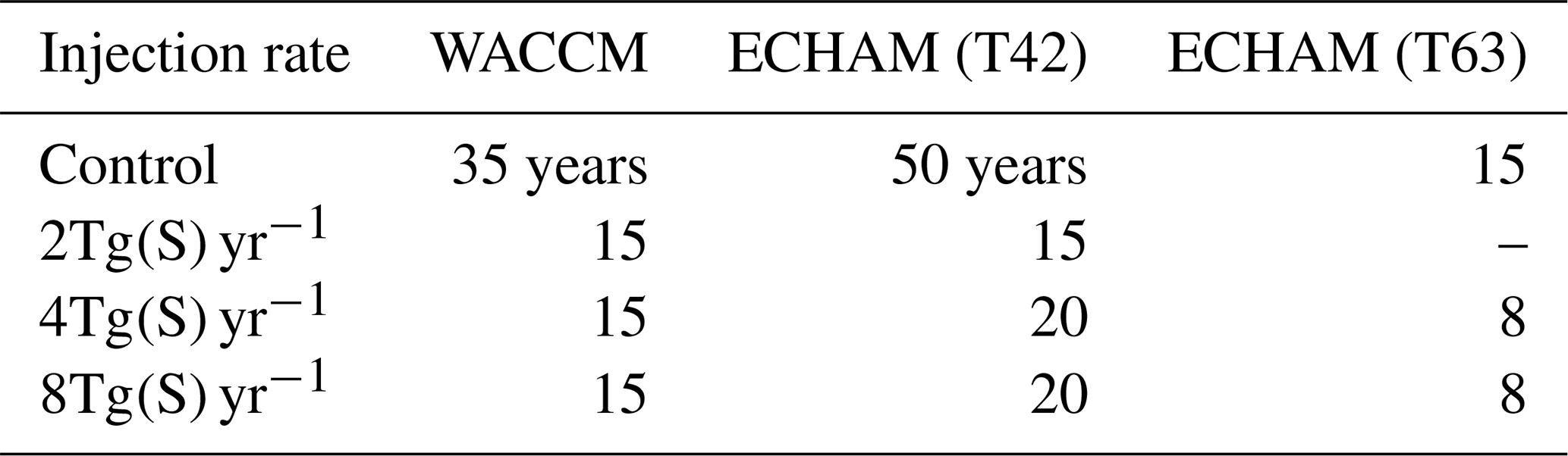
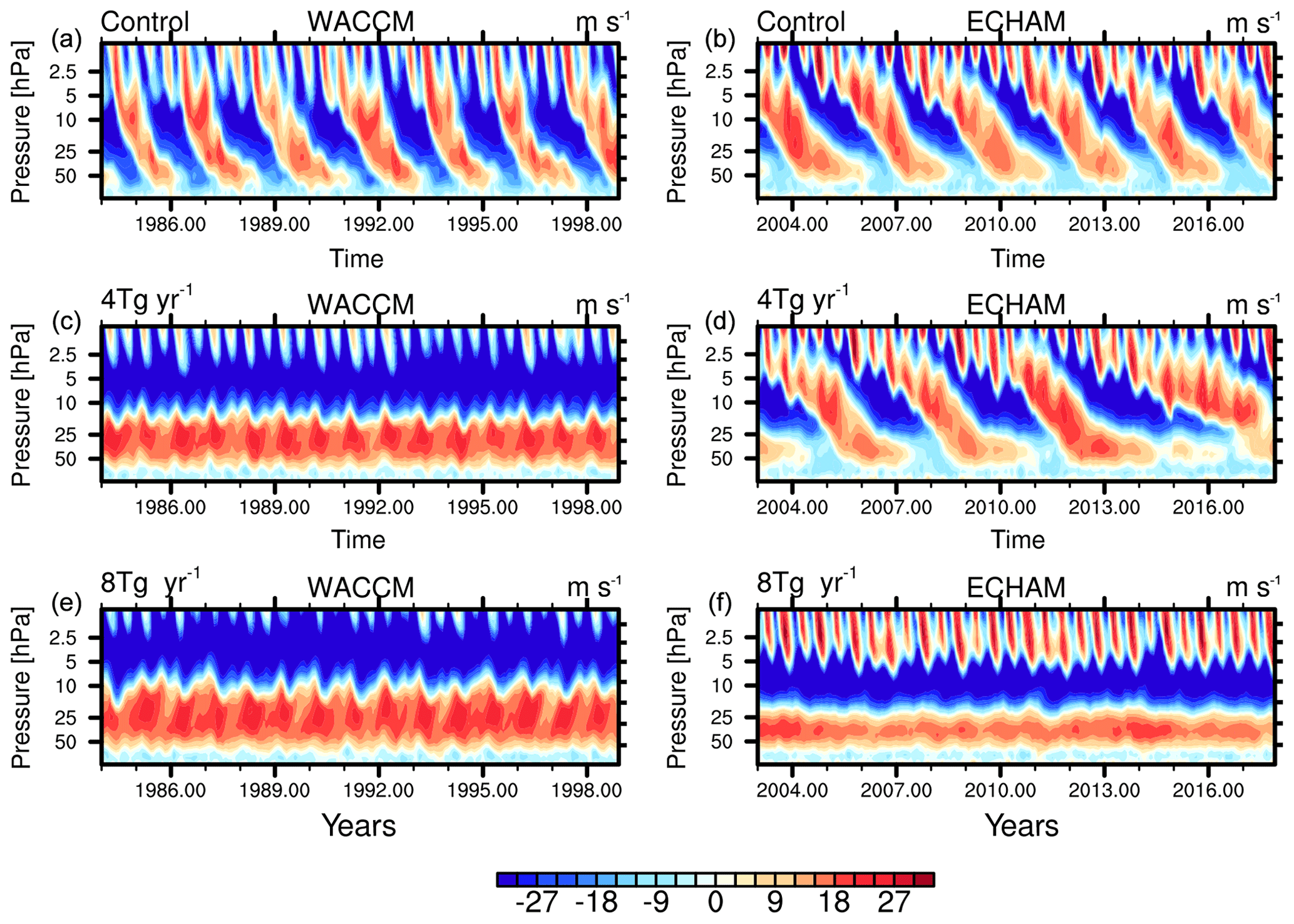
Figure 1 Zonal mean zonal wind [ms⁻¹] at the Equator for a control simulation (a, b) and simulations with sulfur injections of 4 Tg(S) yr⁻¹ (c, d) and 8 Tg(S) yr⁻¹ (e, f). (a, c, e) Results of WACCM. (b, d, f) Results of ECHAM.

3 Results

3.1 QBO changes

Figure 1 shows the zonal mean zonal wind at the Equator for the control simulation and two different injection rates for WACCM and ECHAM. Both models simulate the QBO well in the control simulation, without artificial injections of SO₂ (panels a and b). The QBO has an observed period of 28 months (Naujokat, 1986) on average. The simulated QBO period is about 27 months in WACCM and about 32 months in ECHAM. In WACCM the wind velocity is higher, slightly in the westerly phase but stronger in the easterly phase, especially at altitudes below 20 hPa, and the QBO propagates further down than in ECHAM. After the injection of sulfur into the tropical stratosphere, the QBO responds quite differently to the same injection rate in the two models. While ECHAM shows a slower but still existent oscillation of the zonal wind for injections of 4 Tg(S) yr⁻¹, the oscillation of the zonal wind in WACCM completely vanishes, resulting in constant westerlies in the lower stratosphere and easterlies above ∼10 hPa (Fig. 1c, d). Increasing the injection rate to 8 Tg(S) yr⁻¹ slightly increases the velocity of the westerlies and the vertical extension of the westerly jet in WACCM (Fig. 1e, f). In ECHAM the oscillation vanishes at 8 Tg(S) yr⁻¹ as well, but wind velocity and vertical extension of the westerly jet are lower. The stronger westerly jets in WACCM shift the semi-annual oscillation (SAO) above 5 hPa to higher altitudes. For ECHAM the SAO still reaches 5 hPa for 8 Tg(S) yr⁻¹ injections but gets shifted to higher altitudes, similar to WACCM, when the jets gets stronger with increasing injection rates (Niemeier and Schmidt, 2017). Thus, the QBO disappears in both models as a result of SO₂ injections, but at different injection rates.

3.2 Temperature and heating rate changes

Aquila et al. (2014) identified the absorption of radiation by sulfate aerosols and the consequent heating in the lower stratosphere as the main causes for the changes in the QBO. The heated sulfate layer impacts the thermal wind balance and vertical advection. This heating differs clearly between WACCM and ECHAM as can be seen in the amplitude of temperature anomalies in the stratosphere for both models (Fig. 2). WACCM simulates maxima of temperature anomalies of 5.7 and 12.5 K for injections of 4 and 8 Tg(S) yr⁻¹; ECHAM only simulates 2 and 4.5 K. Thus, for the same sulfur injection rate, WACCM shows a temperature anomaly roughly 3 times stronger than ECHAM. Therefore, the different response of the QBO winds to the injection between the models is not surprising, as the thermal wind balance is much more strongly impacted in WACCM than in ECHAM.

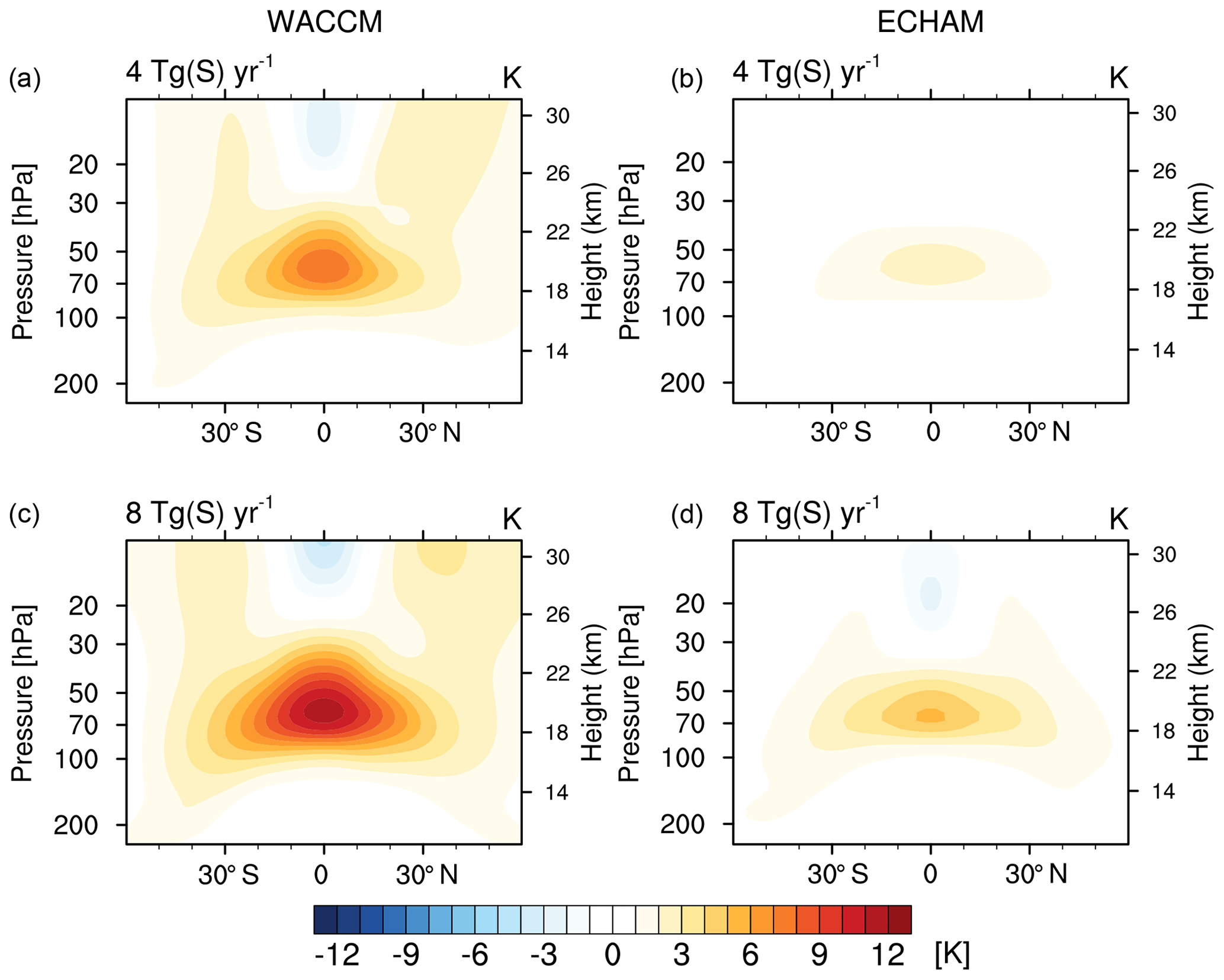
Figure 2 Temperature anomaly (K) caused by injections of 4 Tg(S) yr⁻¹ (a, b) and 8 Tg(S) yr⁻¹ (c, d) of sulfur. (a, c) Results of WACCM. (b, d) Results of ECHAM.

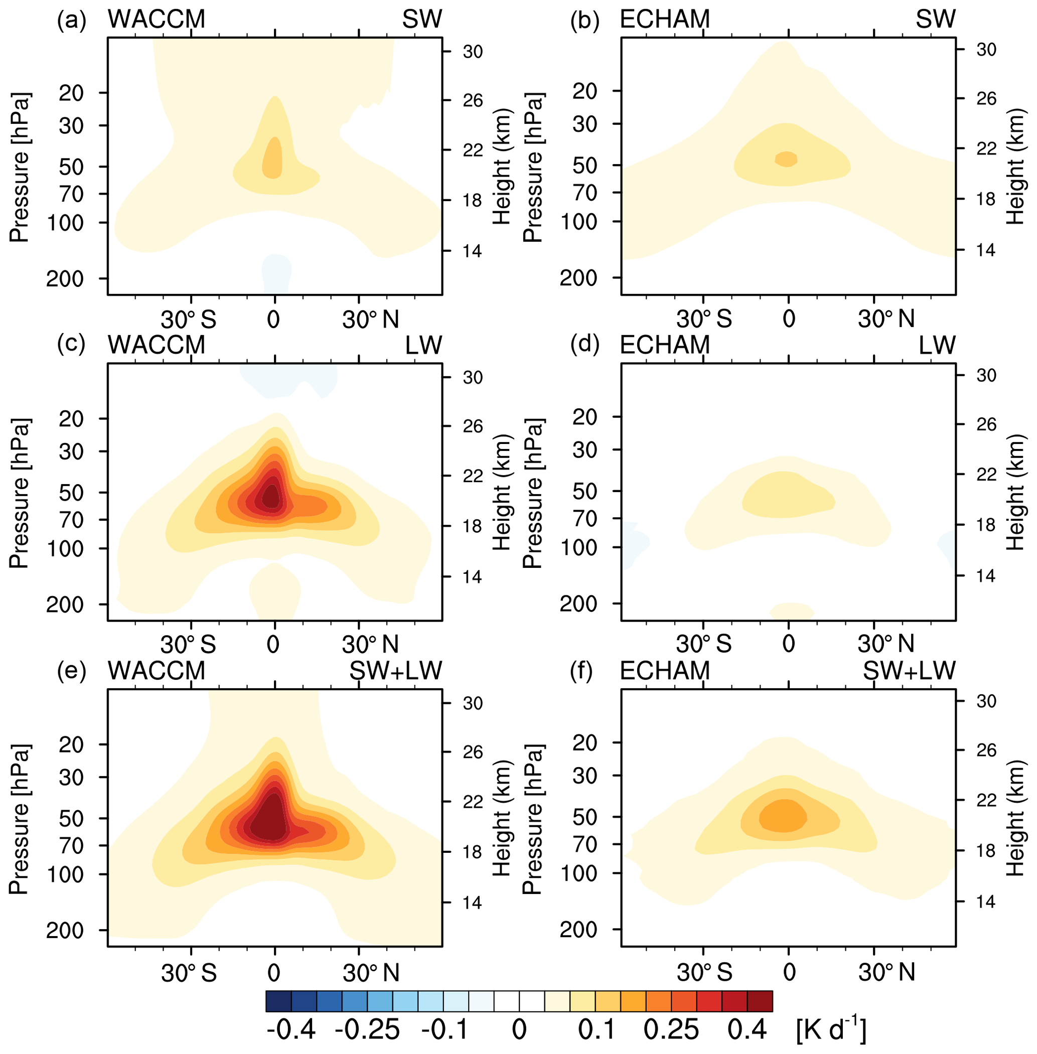
Figure 3 Zonally averaged heating rates of near-infrared (SW, a, b), terrestrial (LW, c, d) and total (e, f) radiation of WACCM (a, c, e) and ECHAM (b, d, f) after an injection of 4 Tg(S) yr⁻¹.

We investigate the reason for the different stratospheric heating in WACCM and ECHAM by examining the SW and LW heating rates in both models for the simulation with 4 Tg(S) yr⁻¹ injection. Similar results are found for the 8 Tg(S) yr⁻¹ simulation and are hence not shown. Splitting of the heating rates into SW and LW components shows that SW heating rates for both models are of comparable amplitude (Fig. 3a, b) whereas there is a clearly higher heating rate for LW radiation than for SW radiation in WACCM (Fig. 3). The heating rates show that WACCM absorbs more than twice as much in the LW than in SW, while absorption is similar in between LW and SW in ECHAM. In total (SW + LW), WACCM absorbs more than twice as much radiation than ECHAM. The stronger heating rate in WACCM corresponds to the stronger temperature anomaly in WACCM. Both models use the same radiation scheme; hence the differences can not be explained by the radiation scheme and must be caused by other processes in the model. For example, the heating rate due to absorption of LW radiation depends on the sulfur mass.

3.3 Sulfate properties

The zonally averaged sulfate burden, the vertically integrated sulfate concentration, shows a higher burden in WACCM at all latitudes than in ECHAM for the injection rate of 4 Tg(S) yr⁻¹ (Fig. 4). WACCM shows a distinct peak at the Equator while in ECHAM the distribution is much more even with latitude, and the secondary maxima, caused by the blocking of meridional transport by the polar vortex in the winter hemisphere, in the extratropics are only slightly smaller than the tropical maximum. The larger temperature anomaly in WACCM, 3 to 4 times larger, can be explained by the larger tropical sulfate burden, as more sulfate aerosols can absorb more radiation.

Figure 4 Zonally averaged sulfate burden of injections of 4 Tg(S) yr⁻¹ for WACCM and ECHAM.

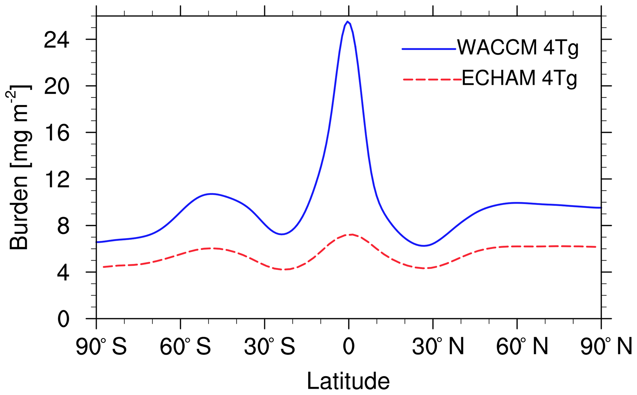
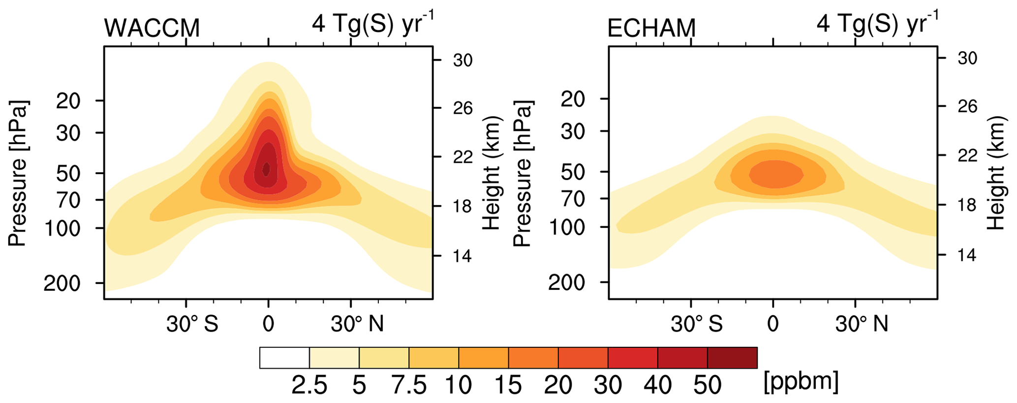
Figure 5 Zonally averaged sulfate concentration (ppbm) of injections of 4 Tg(S) yr⁻¹ for WACCM and ECHAM.

The vertical cross section of the zonally averaged sulfate concentrations reveals more details of the differences in distributions of sulfate in the two models (Fig. 5). Not only is the tropical concentration higher in WACCM, but in addition, the vertical distribution of aerosols is very different between the two models. In ECHAM the sulfate is vertically advected to 25 hPa, while in WACCM sulfate reaches much higher altitudes, and meridional transport mainly occurs below 50 hPa. Vertical advection has to be much stronger in WACCM than in ECHAM to cause the differences. This is likely caused by a combination of a stronger lofting of aerosols as the result of radiative heating by aerosols, as well as resulting changes in the stratospheric wave propagation which cause an increase in the residual vertical velocity. Thus, from the comparison of the sulfur injection cases only, we cannot conclude whether (a) the strong vertical advection is a consequence of the stronger heating or (b) the cause of higher sulfate mass and, consequently, stronger heating. At this point we can only assume that the stronger tropical aerosol heating in WACCM is related to the higher sulfate load. The heating is a consequence of the sulfate burden and not the source of the differences between the two models.

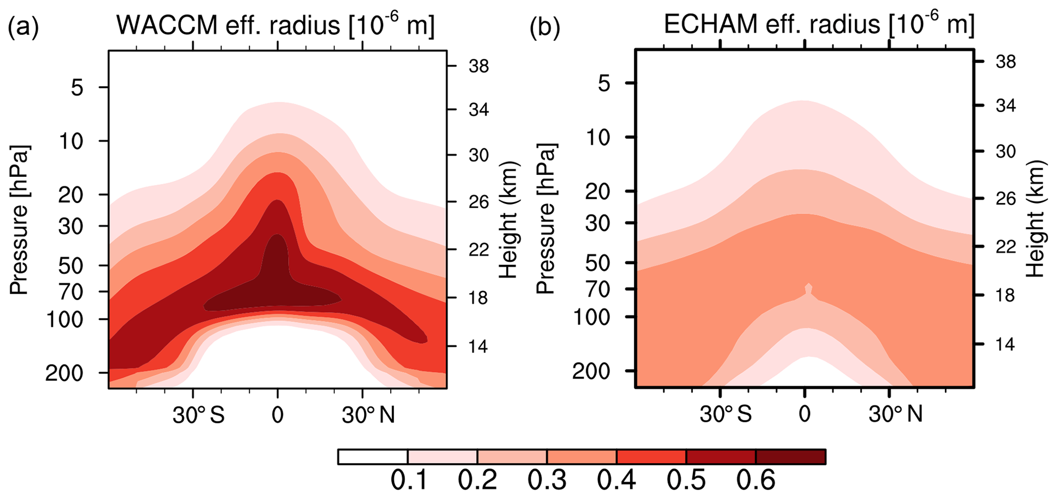
Figure 6 Effective radius (µm) for an injection rate of 4 Tg(S) yr⁻¹ of WACCM (a) and ECHAM-HAM (b). WACCM shows only values in the stratosphere.

To further understand differences in the aerosol distribution and the resulting heating between WACCM and ECHAM, we examine the effective radii of aerosols in both models. This comparison (Fig. 6) shows radii twice as large for WACCM in the tropics (0.6 µm) than for ECHAM (0.3 µm). The higher sulfur load results in larger particle radii, less scattering and less SW radiative forcing (Dykema et al., 2016). LW radiative forcing depends on the sulfate mass and stays constant per injected sulfur unit and is not related to particle radii. From the larger radii in WACCM we may assume a stronger sedimentation in the tropics in WACCM. But the burden is larger in WACCM. If sedimentation is a major difference between the models, the difference in the tropical burden between the two models should be smaller. An additional process which determines the lifetime of the aerosols in the tropics is the vertical advection, the residual vertical velocity ω^∗.

3.4 Dynamical changes

The patterns of the heating rates, sulfate concentrations and particle radii hint towards a stronger vertical advection in WACCM. A proxy for this behavior is the residual vertical velocity, ω^∗. Richter et al. (2017) have shown that vertical advection plays a major role in dynamical changes in the tropical stratosphere. Visioni et al. (2018) showed a strong relation between the sulfate lifetime and ω^∗. Therefore, we compare the residual vertical velocity of the control simulations (Fig. 7) to get a more general impression of the behavior of the two models, independently of additional updraft caused by the aerosol heating. In the altitude of the sulfur injection (60 hPa), WACCM shows an up to 70 % stronger ω^∗ than ECHAM. This stronger ω^∗ results in a stronger vertical transport of the sulfate aerosols, which increases the tropical sulfate burden in WACCM. Additionally, the minimum of the ω^∗ profile is located at lower altitude in WACCM (70 and 50 hPa in ECHAM), resulting in a stronger tropical confinement of the aerosols at this altitude.

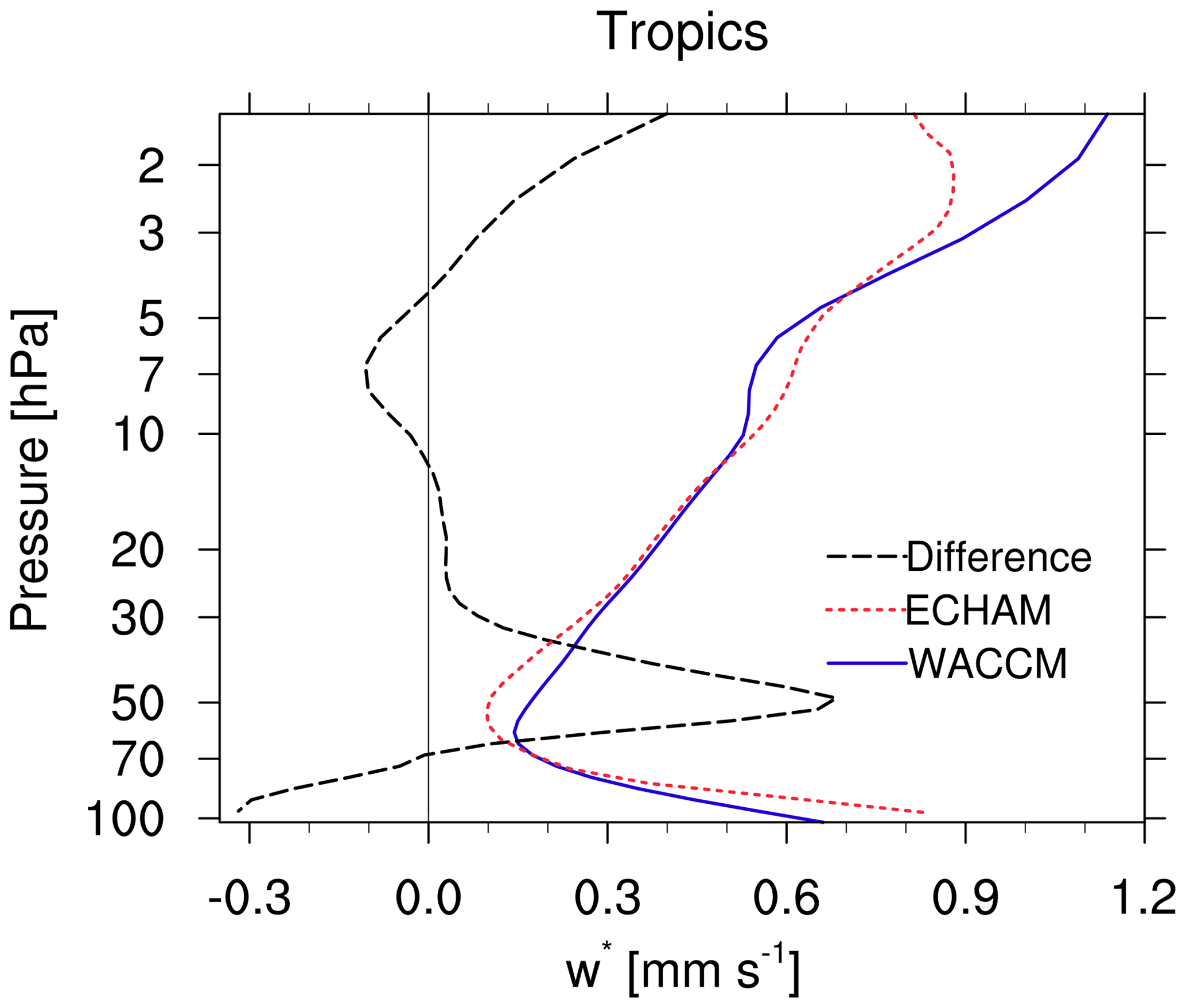
Figure 7 Residual vertical velocity of the control simulations in the tropics (averaged over 5^∘ N to 5^∘ S). Results of ECHAM (red) and WACCM (blue), and in black the difference – (WACCM−ECHAM)∕ECHAM.

Figure 8 Residual vertical velocity in the tropics for the control simulation and simulations with injections of 2, 4 and 8 Tg(S) yr⁻¹ for WACCM (a) and ECHAM (b).

The consequence is twofold: (a) a stronger ω^∗ counteracts more the downward propagation of the QBO shear zones and (b) lifts the aerosols to higher altitudes, which increases the burden and thus causes stronger heating. The heating of the aerosols further increases ω^∗, which shifts the minimum of ω^∗ downward (Fig. 8). This can be seen in both models, but stronger in WACCM than in ECHAM. This feedback loop finally results in the vanishing of the QBO at an injection rate of 2 Tg(S) yr⁻¹ in WACCM compared to 8 Tg(S) yr⁻¹ in ECHAM. The reasons for the differences in ω^∗ in the control may lie in differences in the gravity wave parameterization and the relation of how strongly resolved Rossby waves or parameterized gravity waves drive the upward mass flux (Cohen et al., 2014; SPARC, 2010). The better grid resolution in WACCM may also play a role. We conclude that the stronger ω^∗ in WACCM is the main reason for the differences between the QBO response in the two models.

3.5  Comparison under the same heating conditions

Are differences in ω^∗ between the models the main cause of the difference in QBO impact or does the different heating also play an important role? To answer this question we compare different sulfur injection rates in the models that produce a similar heating rate in the sulfate layer. An injection rate of 2 Tg(S) yr⁻¹ in WACCM and 8 Tg(S) yr⁻¹ in ECHAM fulfills this criterion (Fig. 9a, b). Both experiments result in a temperature anomaly of ∼4 K in the tropical stratosphere. The heated area is slightly wider in ECHAM because the sulfate concentration (Fig. 9c, d) is slightly higher in the tropics and spreads more meridionally around 50 hPa. However, the maximum burden between the two models is rather similar in the tropics (Fig. 10). The tropical maximum of the sulfate burden in ECHAM is only 2 mg m⁻² (12 %) higher than in WACCM, despite an injection rate of sulfur a factor of 4 higher. The differences in the burden are larger in the extratropics (∼50 %). But the extratropical differences are not the focus of this study as we focus on the tropical stratosphere and the QBO.

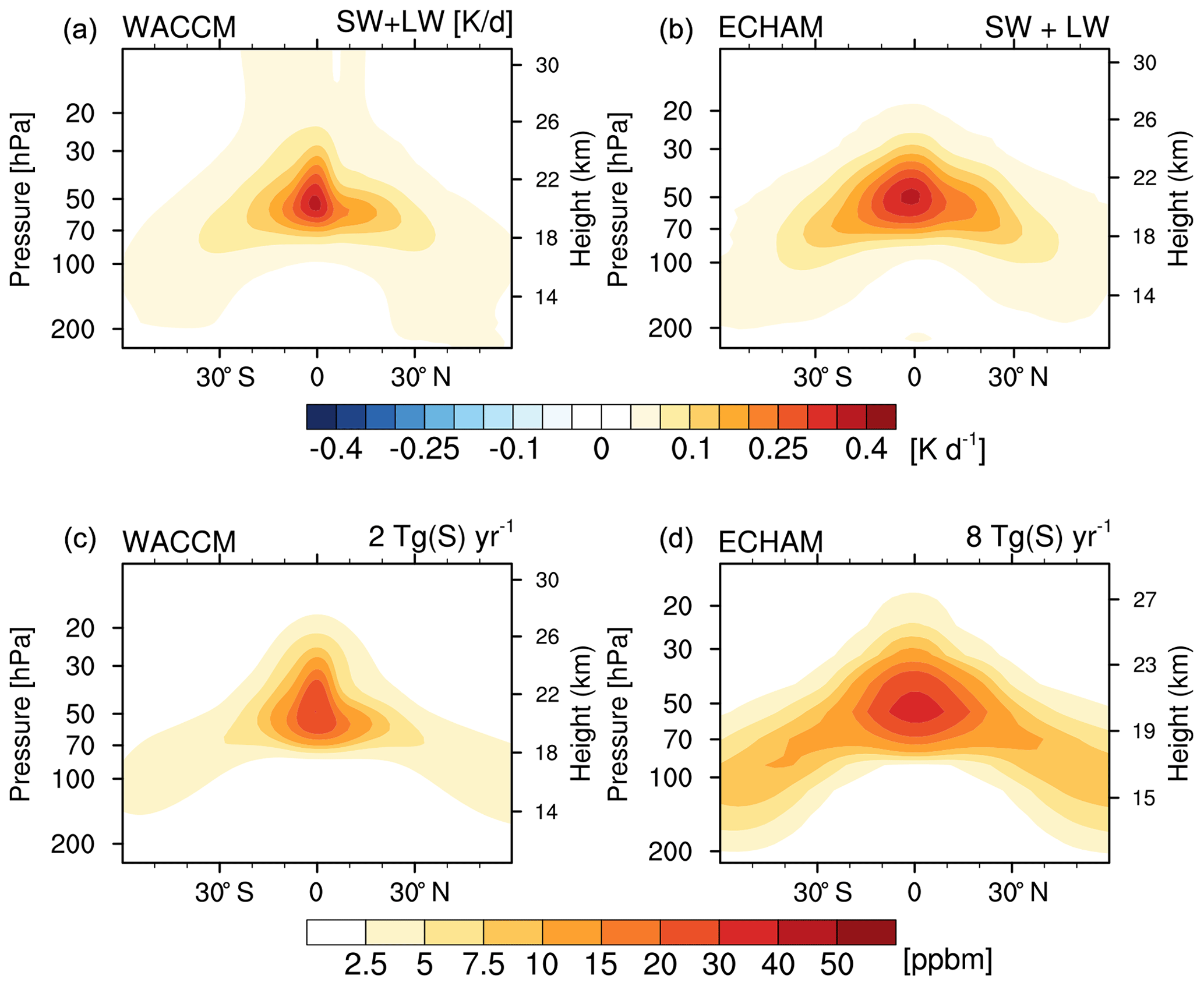
Figure 9 (a, b) Heating rate (K d⁻¹) and (c, d) sulfate concentration of a 2 Tg(S) yr⁻¹ injection rate in WACCM (a, c) and an 8 Tg(S) yr⁻¹ injection rate in ECHAM (b, d). Injection rates were chosen to result in similar temperature anomalies in both models. Intervals of the heating rates (a, b) are 0.01, 0.05, 0.1, 0.15, 0.2, 0.25, 0.3, 0.35 and 0.4 K d⁻¹.

Figure 10 Zonally averaged sulfate burden of a 2 Tg(S) yr⁻¹ injection rate in WACCM (blue) and an 8 Tg(S) yr⁻¹ injection rate in ECHAM-HAM (red, dashed).

The continuous westerly and easterly jets cause a different profile of ω^∗ than oscillating zonal winds under QBO conditions (Fig. 8). The clearly different profile of ω^∗ for the low-injection cases to the 8 Tg(S) yr⁻¹ in ECHAM and for all three injection cases to the control in WACCM is a consequence of the disappearance of the QBO. We see a strong correlation of the pattern of the residual vertical velocity to the equatorial zonal wind profiles (Fig. 1). The characteristic pattern of the vertical profile of ω^∗ in WACCM becomes similar in ECHAM-HAM when the oscillation of the equatorial jets vanishes at 8 Tg(S) yr⁻¹ (Fig. 8). Consequently, the maximum difference of ω^∗ between the models is only 34 % within the sulfate layer (80 to 20 hPa when comparing the 2 Tg(S) yr⁻¹ WACCM and the 8 Tg(S) yr⁻¹ ECHAM injection cases (Fig. 11). Differences occur mostly due to a vertical shift in the profiles. The constant easterly and westerly jets cause distinct maxima and minima of ω^∗ below 50 hPa. This compares well to the theory of the meridional and vertical transport processes within the QBO region and the secondary meridional oscillation (Plumb and Bell, 1982), which is caused by equatorward meridional advection in westerly jets and poleward meridional advection within easterly jets combined with updraft in easterly shear and downdraft in westerly shear. For example, the positions of the maxima around 30 and 20 hPa are the transition zones of the westerly and easterly jets. The heating of the aerosols, and the corresponding increased ω^∗, interferes with downdraft tendency in the westerly shear zone below 50 hPa. The result is that the ω^∗ minimum around 60 hPa and the maximum between 30 and 10 hPa align with the easterly shear zone (Fig. 12).

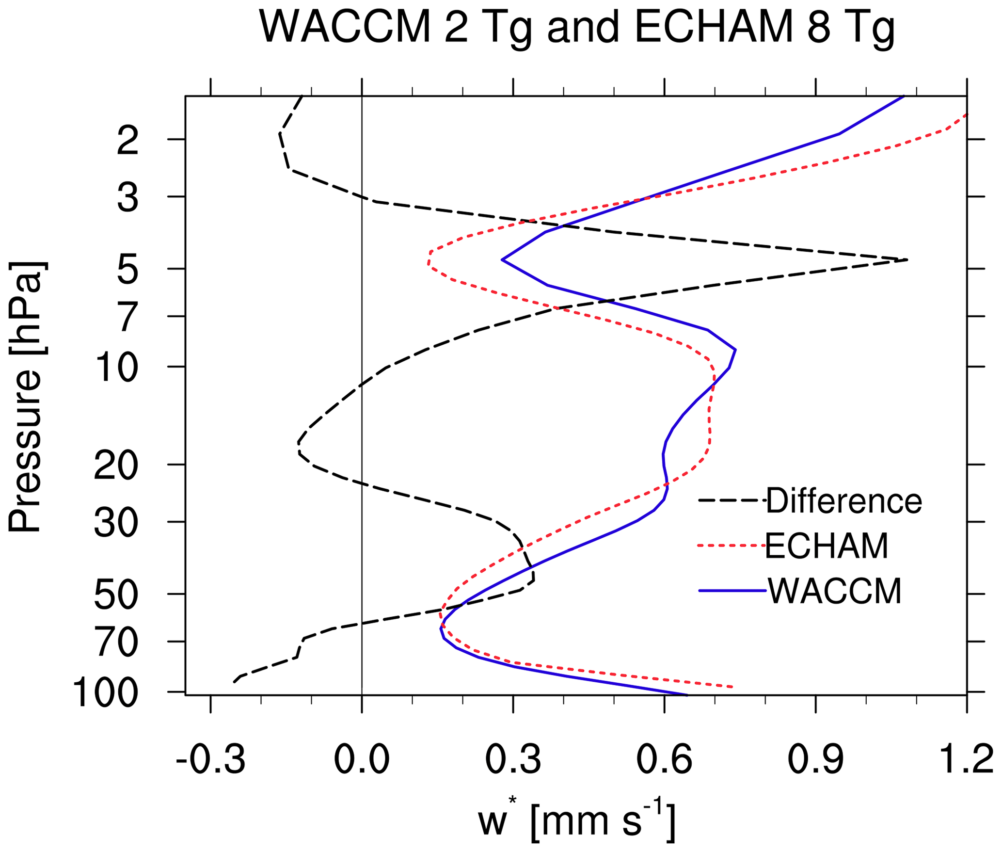
Figure 11 Residual vertical velocity in the tropics for a WACCM simulation with an injection rate of 2 Tg(S) yr⁻¹ (blue), ECHAM simulation with an injection rate of 8 Tg(S) yr⁻¹ (red) and the difference (black, (WACCM−ECHAM)∕ECHAM).

Finally, we can say that the similar heating anomalies result in very similar zonal winds at the Equator in both models (Fig. 12). Both models show the vanishing of the QBO with a westerly jet in the lower stratosphere combined with an easterly jet at higher altitudes. WACCM simulates slightly higher wind velocities and less vertical extension of the westerly jet than ECHAM, but in general the response of the two models is very similar. Our findings suggest that the stronger tropical aerosol heating in WACCM is a consequence of the higher sulfate concentrations. The source of the differences between the two models, and the cause of the higher concentrations in WACCM, is the different ω^∗.

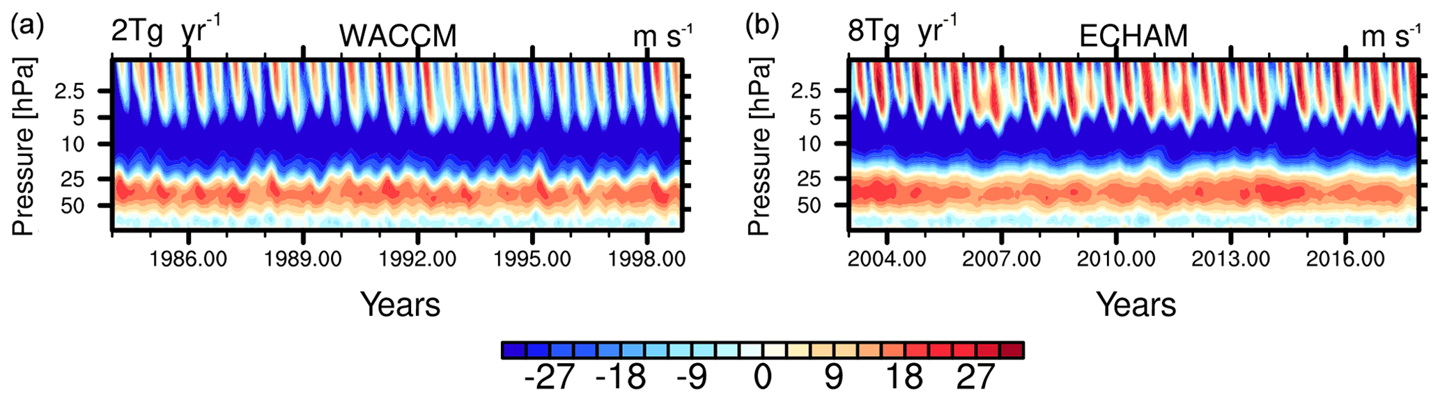
Figure 12 Zonal mean zonal wind at the Equator of a 2 Tg(S) yr⁻¹ injection rate in WACCM (b) and an 8 Tg(S) yr⁻¹ injection rate in ECHAM.

3.6 Impact of grid resolution

The horizontal resolution of the two models is very different in this study, ∼1^∘ for WACCM and ∼2.8^∘ for ECHAM. Therefore, we examine the importance of different horizontal model resolutions on our results to reduce the number of uncertainties in our comparison. We increased the resolution of ECHAM from T42 to T63 (∼1.8^∘). This is still a coarser horizontal resolution than in WACCM but differences between the two simulations of ECHAM can indicate the impact of the horizontal resolution on the transport of sulfate out of the tropics and on the QBO.

When comparing the vertical velocity of T42 and T63 control simulations of ECHAM in the tropics (Fig. 13a), we get a slight increase in ω^∗ (16 %) in T63 in the area of the sulfate layer around an altitude of 50 hPa. This is much smaller than the difference to WACCM. Thus, we could expect a still smaller ω^∗ in ECHAM in the case of a similar horizontal resolution. But we also see a slight shift of the minimum of ω^∗ to a lower altitude. From the differences to WACCM, the minimum of ω^∗ being at a lower altitude in WACCM, we can expect a stronger confinement of the aerosols in the tropics. Indeed we find that the horizontal resolution has an impact on the simulated burden (Fig. 13b). The burden is about 30 % higher in the tropics for injections of 8 Tg(S) yr⁻¹ in the T63 simulation compared to the T42 simulation. The 4 Tg(S) yr⁻¹ burden comes closer to the 2 Tg(S) yr⁻¹ results of WACCM, with a substantial reduction of the peak in the aerosol burden in the tropics, but does not cause the QBO to vanish (not shown).

Figure 13 (a) Residual vertical velocity in the tropics of control simulations of ECHAM with T42 and T63 resolution. (b) Zonally averaged sulfate burden of WACCM (blue) and ECHAM T63 (dashed) and T42 (solid).

The vertical resolution of the models differs as well: 110 levels in WACCM and 90 levels in ECHAM. Within the area of interest however, between 100 and 10 hPa, the number of model levels is very similar: 32 levels for WACCM and 27 levels for ECHAM, with approximate grid spacing of 0.5 km for WACCM and 0.6 km for ECHAM. We do not expect a strong impact on ω^∗ from this small difference in vertical resolution.

Horizontal resolution seems to play a bigger role in the simulation of ω^∗. Increasing the resolution to T63 leads to a polar shift of the midlatitude westerlies in the troposphere (Roeckner et al., 2006) with consequences for large-scale wave propagation into the stratosphere. The dynamical changes result in an increase in the sulfate burden at all latitudes, not only in the tropics. The pattern of the burden indicates a slightly smaller residual meridional velocity and different isentropic mixing in the midlatitudes in T63. Additionally, Brühl et al. (2018) describe a better representation of sedimentation processes at high latitudes in T63. As we concentrate on the impact of sulfate on the QBO in this study, the differences in the extratropics will be left for further studies.

4 Summary and discussion

We performed here simulations with different injection rates of SO₂ at the Equator to compare the impact on the QBO in two different general circulation models (WACCM and ECHAM). The QBO typically consists of alternating easterly and westerly zonal mean zonal winds; however in the presence of sulfur injections, the QBO sometimes vanishes and turns into persistent westerlies in the lower stratosphere and persistent easterlies in the upper stratosphere. Both models used in the study had a similar setup (e.g., prescribed SSTs and present-day chemical precursors like OH or ozone) and were coupled to an aerosol microphysical model with three modes in WACCM and four modes in ECHAM. Both models qualitatively simulate an impact on the QBO of sulfur injections similar to what was found in previous studies (Niemeier and Schmidt, 2017; Richter et al., 2017); however WACCM shows a disappearance of the QBO at an injection rate of 2 Tg(S) yr⁻¹ whereas ECHAM shows the disappearance of the QBO for an injection rate of 8 Tg(S) yr⁻¹.

We have shown that this difference results from different tropical vertical advection and different tropical residual vertical velocity, ω^∗, in the two models. ω^∗ differs not only in the simulations with SO₂ injections, but also in the control simulations without any sulfur injection. In WACCM, ω^∗ is 70 % larger than in ECHAM near the altitude of the SO₂ injection. Additionally, the minimum of ω^∗ is located at a lower altitude. At altitudes with a small ω^∗ meridional transport is enhanced, while a strong ω^∗ causes an enhanced tropical confinement of the aerosols. This confinement is stronger in WACCM above 50 hPa. Thus, the stronger ω^∗ results in a stronger vertical lifting, higher sulfate burden and consequently stronger heating of the stratosphere caused by aerosol absorption. This heating disturbs the thermal wind balance and causes an additional westerly momentum. Finally, this results in the disappearance of the QBO at lower SO₂ injection rates than in ECHAM. This result partly opposes the assumptions of Kleinschmitt et al. (2017), who assumed the heating to be the main cause for different vertical advection in two models. It would be interesting to compare our results to the ω^∗ of their control simulation.

In this study we compared injections at 60 hPa (about 19 km) only. This altitude shows the largest differences in ω^∗ between the two models of all altitudes. Therefore, injections at higher altitude, e.g., 30 hPa (24 km) would, most probably, cause fewer differences. Comparing results of Niemeier and Schmidt (2017) and Tilmes et al. (2018), both show results of injections at two altitudes and smaller differences between the models for the higher-altitude injections.

The reason for the different ω^∗ in the two models is complex. ω^∗, or the speed of the upwelling in the Brewer–Dobson circulation, is driven by a combination of larger-scale waves (Rossby and synoptic-scale waves) and parameterized waves. The propagation of waves and deposition of wave momentum by larger-scale waves are impacted by numerous aspects of the model such as horizontal and vertical resolution, diffusion parameterization and physics parameterizations, which all differ between WACCM and ECHAM. Gravity wave parameterization contributions to driving the Brewer–Dobson circulation also vary between models (Butchart et al., 2011). WACCM and ECHAM have very different gravity wave parameterizations. It would thus be very difficult to isolate the reason for the different ω^∗ between WACCM and ECHAM, but simulations with different horizontal resolution shown in Sect. 3.6 have shown that the horizontal resolution difference between WACCM and ECHAM contributed to the differences in ω^∗. Additionally, sedimentation may differ between the models as might be concluded from the difference in deposition when simulating a Tambora-like volcanic eruption (Marshall et al., 2018). Sedimentation is a very important sink process for aerosols, especially at the poles, but three-dimensional fields of sedimentation velocities were not available for both models. As we concentrated on the tropical stratosphere only, we leave this topic for further studies.

Finally we conclude that the difference in tropical upwelling even under present climate conditions between two models has a major impact on the projected effects of SO₂ injections on the QBO in WACCM and ECHAM. This is worrisome in terms of the level of certainty of effects of SO₂ injections on stratospheric circulation in future climates, especially as the changes in the Brewer–Dobson circulation are uncertain. In addition changes in gravity waves, which are a big driver of the QBO, are even more uncertain in changing climate. The model intercomparison initiative GeoMIP6 (Kravitz et al., 2015) has mainly concentrated on climate impact of CE. A simple SO₂ injection experiment with well-defined input parameters for GCMs with aerosol microphysical modules, e.g., grid resolution, injection and model setups, may create further understanding of related differences and uncertainties. Hence, a lot more research is needed before agreement is reached on how SO₂ injections could affect the QBO. The reasons for the differences in this variable are too complex to provide a solution for a better agreement of the results.