Global distribution and 14-year changes in erythemal irradiance, UV atmospheric transmission, and total column ozone for2005–2018 estimated from OMI and EPIC observations

Satellite data from the Ozone Measuring Instrument (OMI) and Earth Polychromatic Imaging Camera (EPIC) are used to study long-term changes and global distribution of UV erythemal irradiance $E(\mathit{\zeta },\mathit{\phi },z,t)$ (mW m⁻²) and the dimensionless UV index E ∕ (25 m Wm⁻²) over major cities as a function of latitude ζ, longitude φ, altitude z, and time t. Extremely high amounts of erythemal irradiance (12 < UV index <18) are found for many low-latitude and high-altitude sites (e.g., San Pedro, Chile, 2.45 km; La Paz, Bolivia, 3.78 km). Lower UV indices at some equatorial or high-altitude sites (e.g., Quito, Ecuador) occur because of persistent cloud effects. High UVI levels (UVI > 6) are also found at most mid-latitude sites during the summer months for clear-sky days. OMI time-series data starting in January 2005 to December 2018 are used to estimate 14-year changes in erythemal irradiance ΔE, total column ozone ΔTCO₃, cloud and haze transmission ΔC_T derived from scene reflectivity LER, and reduced transmission from absorbing aerosols ΔC_A derived from absorbing aerosol optical depth τ_A for 191 specific cities in the Northern Hemisphere and Southern Hemisphere from 60^∘ S to 60^∘ N using publicly available OMI data. A list of the sites showing changes at the 1 standard deviation level 1σ is provided. For many specific sites there has been little or no change in $E(\mathit{\zeta },\mathit{\phi },z,t)$ for the period 2005–2018. When the sites are averaged over 15^∘ of latitude, there are strong correlation effects of both short- and long-term cloud and absorbing aerosol change as well as anticorrelation with total column ozone change ΔTCO₃. Estimates of changes in atmospheric transmission ΔC_T (ζ, φ, z, t) derived from OMI-measured cloud and haze reflectivity LER and averaged over 15^∘ of latitude show an increase of 1.1±1.2 % per decade between 60 and 45^∘ S, almost no average 14-year change of 0.03±0.5 % per decade from 55^∘ S to 30^∘ N, local increases and decreases from 20 to 30^∘ N, and an increase of 1±0.9 % per decade from 35 to 60^∘ N. The largest changes in $E(\mathit{\zeta },\mathit{\phi },z,t)$ are driven by changes in cloud transmission C_T. Synoptic EPIC radiance data from the sunlit Earth are used to derive ozone and reflectivity needed for global images of the distribution of $E(\mathit{\zeta },\mathit{\phi },z,t)$ from sunrise to sunset centered on the Americas, Europe–Africa, and Asia. EPIC data are used to show the latitudinal distribution of $E(\mathit{\zeta },\mathit{\phi },z,t)$ from the Equator to 75^∘ for specific longitudes. EPIC UV erythemal images show the dominating effect of solar zenith angle (SZA), the strong increase in E with altitude, and the decreases caused by cloud cover. The nearly cloud-free images of $E(\mathit{\zeta },\mathit{\phi },z,t)$ over Australia during the summer (December) show regions of extremely high UVI (14–16) covering large parts of the continent. Zonal averages show a maximum of UVI = 14 in the equatorial region seasonally following latitudes where SZA = 0^∘. Dangerously high amounts of erythemal irradiance (12 < UV index < 18) are found for many low-latitude and high-altitude sites. High levels of UVI are known to lead to health problems (skin cancer and eye cataracts) with extended unprotected exposure, as shown in the extensive health statistics maintained by the Australian Institute of Health and Welfare and the United States National Institute of Health National Cancer Institute.

1 Introduction

Calculated and measured amounts of UV radiation reaching the Earth's surface can be used as a proxy to estimate the combined effects of changing ozone, aerosols, and cloud cover on human health. High levels of UV irradiance, usually occurring at small solar zenith angles (SZAs) or high altitudes, are known to affect the incidence of skin cancer and the development of eye cataracts (Findlay, 1928; Diffey, 1987; Strom and Yamamura, 1997; Ambach and Blumthaler, 1993; Abraham et al., 2010; Roberts, 2011; Behar-Cohen, 2014; Watson et al., 2016; Australian Institute of Health and Welfare, 2016; Howlander et al., 2019; US Department of Health and Human Services, 2018).

The UV response functions (action spectra) for the development of skin cancer and eye cataracts are different (Herman, 2010), but the effects are highly correlated. Similar correlations exist for other action spectra (e.g., plant growth, vitamin D production, and DNA damage action spectra) involving the UV portion of the solar spectrum. Because of these correlations, this paper will only estimate erythemal (skin reddening) effects. To obtain standardized results, we use a weighted UV spectrum (290–400 nm) based on the CIE-action (Commission Internationale de l'Eclairage) spectrum suggested by McKinlay and Diffey (1987) to estimate the erythemal effect of UV radiation incident on human skin. Erythemal irradiance (E) is usually measured or calculated in energy units (mW m⁻²) or in terms of the UV index UVI = E ∕ (25 mW m⁻²), reaching the Earth's surface after passing through atmospheric absorbing and scattering effects from ozone, aerosols, and clouds.

Previous work (Krotkov et al., 1998, 2001; Gao et al., 2001; Arola et al., 2005, 2009; Seckmeyer et al., 2006; Tanskanen, et al., 2007; Bernhard et al., 2010; Herman, 2010) includes extensive analysis of UV irradiance at the Earth's surface from satellites and ground-based instruments for individual irradiance wavelengths and weighted with various action spectra. One of the chapters in Bernhard et al. (2010) provides references to the National Science Foundation's database of Antarctic region UV instruments including measurements of the daily maximum UVI from Ushuaia, Argentina, with values of 8–9 for January 2008 and approximately 11 for San Diego, California, in June. Similar data are available for different years from the Brewer spectroradiometer WOUDC site https://woudc.org/data/stations/ (last access: 16 June 2020).

Eleftheratos et al. (2015) give estimates of UV trends at northern high latitudes showing a decrease of 3.9 % at 305 nm with little change at 325 nm for the period 1990–2011, suggesting that the change is caused by increasing ozone amounts, not cloud cover changes. No statistically significant changes in 307.5 or 350 nm UV irradiance were found for Thessaloniki for the period 2006–2014 (Fountoulakis et al., 2016). A decrease in erythemal irradiance was observed for Chilton, UK, of 1 % yr⁻¹ from 2000 to 2015 (Hooke et al., 2015). An analysis of OMI (Ozone Monitoring Instrument onboard the NASA AURA spacecraft) erythemal irradiance estimates without absorbing aerosols (Tanskanen, et al., 2007) compared to ground-based measurements found that “For flat, snow-free regions with modest loadings of absorbing aerosols or trace gases, the OMI-derived daily erythemal doses have a median overestimation of 0 %–10 %, and some 60 % to 80 % of the doses are within ±20 % from the ground reference.” An OMI erythemal data set (Tanskanen, et al., 2006, 2007) is available for different sites than used in the current study using the same OMI ozone data but different cloud C_T and absorbing aerosol C_A transmission factors. For C_A in this study, the 354 nm absorbing aerosol optical depth τ_A can be obtained from the $\mathrm{1}{}^{\circ }\times \mathrm{1}{}^{\circ }$ absorbing aerosol data set: https://disc.gsfc.nasa.gov/datasets/OMAEROe_003/summary?keywords=omi (last access: 16 June 2020).

Lindfors et al. (2009) published a global erythemal analysis based on pseudo-spherical radiative transfer that includes absorbing aerosol optical depth τ_A from a climatology and combined ozone and cloud data from multiple satellites. A similar aerosol absorption algorithm has been proposed for ESA/EU Copernicus Sentinel 5 precursor (S5P/TROPOMI) (Lindfors et al., 2018) using a form $E\left({\mathit{\tau }}_{\mathrm{A}}\right)=E\left(\mathrm{0}\right)/(\mathrm{1}+\mathrm{3}{\mathit{\tau }}_{\mathrm{A}})$ originally empirically derived by Krotkov et al. (2005) to improve the agreement between radiative transfer calculations using satellite data and ground-based irradiance measurements using the absorption optical depths τ_A derived from OMI-measured radiances (Torres et al., 2007).

The radiative transfer algorithm (Herman et al., 2018, and in the Appendix) used in this study has been extended to include the effect of increasing E with altitude and decreases from aerosol absorption (Eqs. 1–3). The method is applied to both OMI total column ozone TCO₃ and Lambert equivalent reflectivity LER (LER accounts for both clouds and scattering aerosols) measured at $\mathrm{13}:\mathrm{30}\pm \mathrm{00}:\mathrm{30}$ and the synoptic measured amounts of TCO₃ and LER obtained from the EPIC (Earth Polychromatic Imaging Camera) instrument onboard the DSCOVR (Deep Space Climate Observatory) spacecraft orbiting about the Earth–Sun Lagrange-1 gravitational balance point (Herman et al., 2018; Marshak et al., 2018). The EPIC global synoptic sunrise to sunset estimates of E(t_O) augment the specific site locations selected for OMI local noon time-series analysis. The synoptic views are derived from simultaneous EPIC measurements of the illuminated Earth at various Greenwich Mean Times t_O with a spatial resolution of 18×18 km² at the spacecraft nadir view centered on various longitudes each 24 h period.

This paper presents calculated noontime $E(\mathit{\zeta },\mathit{\phi },z,t)$ time series and estimated least squares (LS) trends (2005–2018) from a multivariate linear regression model (Randel and Cobb, 1994) for globally distributed locations at different latitudes ζ, longitudes φ, altitudes z, and time t (in years), most of which are centered over heavily populated areas such as New York City, Seoul, Korea, and Buenos Aires (see Tables 1–4 and an extended Table A4 in the Appendix) based on measurements of the relevant parameters from OMI. OMI satellite measurements were selected for trend estimates (percent change per year) because OMI has the longest continuous well-calibrated UV irradiance time series from a single instrument (Schenkeveld et al., 2017) with global coverage and moderate spatial resolution (13×24 km² at its nadir view). Since the main goal of this study is to estimate the long-term changes in E (% yr⁻¹) over a selection of major cities, estimates are given of 14-year latitude-dependent changes in atmospheric transmission C_T(ζ, φ, z, t) (mostly from change in cloud reflectivity), changes in total column ozone TCO₃(ζ, φ, z, t), changes in absorbing aerosol transmission C_A(ζ, φ, z, t), and changes in erythemal irradiance $E(\mathit{\zeta },\mathit{\phi },z,t)$. The effect of snow and ice on the surface reflectivity R_G during winter months has been ignored in this study. This means that the already low amounts of erythemal irradiance during high solar zenith angle winter months for high-latitude cities are further underestimated.

1.1 UV-absorbing aerosols

The algorithm used to estimate E in this study is a fast polynomial fit algorithm FP (Herman, 2010, 2018) based on calculations using the scalar TUV radiative transfer program (Madronich, 2007, 1993a, b; Madronich and Flocke, 1997) with a reduction factor for clouds C_T. The FP algorithm used to estimate E has been enhanced to include the effect of aerosol absorption on UV irradiance based on derived 354 nm aerosol optical depths and single scattering albedo from OMI-measured radiances (Torres et al., 2007). The measured absorbing OMI aerosol optical depths τ_A (354 nm) corresponding to the locations in Table A4 are available from https://avdc.gsfc.nasa.gov/pub/DSCOVR/TimeSeries_Absorbing_Aerosol_Data/ (last access: 16 June 2020). The accuracy of OMI-retrieved aerosol properties has been evaluated by comparison to AERONET (AErosol RObotic NETwork) ground-based observations (Ahn et al., 2014; Jethva et al., 2014).

The wavelength λ dependence of τ_A is approximately given by using the absorption Angström exponent A_AE=1.8 derived from data obtained over Seoul, Korea, in a manner similar to that derived for Santa Cruz, Bolivia (Mok et al., 2018).

$$\begin{array}{}\text{(1)}& {\displaystyle \frac{{\mathit{\tau }}_{\mathrm{A}}\left(\mathit{\lambda }\right)}{{\mathit{\tau }}_{\mathrm{A}}\left(\mathrm{354}\mathrm{nm}\right)}}={\left[{\displaystyle \frac{\mathit{\lambda }}{\mathrm{354}}}\right]}^{-\mathrm{1.8}}\end{array}$$

The reduction factor C_A for irradiance E caused by absorbing aerosols is given by Eq. (2).

$$\begin{array}{}\text{(2)}& C_{\mathrm{A}}=E\left({\mathit{\tau }}_{\mathrm{A}}\right(\mathit{\lambda }\left)\right)/E\left(\mathrm{0}\right)=\mathrm{1}/(\mathrm{1}+\mathrm{3}{\mathit{\tau }}_{\mathrm{A}}(\mathit{\lambda }\left)\right)\end{array}$$

For the purposes of estimating the absorption optical depth for erythemal irradiance, a single wavelength, λ=310 nm, is used approximately corresponding to the maximum of the product of solar flux at the Earth's surface and the erythemal action spectrum (Eq. A2).

$$\begin{array}{}\text{(3)}& {\mathit{\tau }}_{\mathrm{A}}\left(\mathrm{310}\mathrm{nm}\right)=\mathrm{1.27}{\mathit{\tau }}_{\mathrm{A}}\left(\mathrm{354}\mathrm{nm}\right)\end{array}$$

1.2 Comparison with previous results

Table 1 shows a comparison of the June maximum local noon UVI values estimated from OMI TCO₃ and LER data with June ground-based measurement data. June was selected for the comparisons, since the SZA changes slowly near solstice, permitting at least a week's data to be considered selecting a maximum that can be compared with comparable calculated erythemal irradiance calculated from OMI data. The day-to-day measured and calculated variation at solar noon during June is greater than 10 % for nearly clear-sky days. Calculated values are 14-year June average maximum values that vary slightly year to year.

Table 1 Comparison of FP-calculated OMI UVI with ground-based measurements.

¹ https://uvb.nrel.colostate.edu/UVB/da_Erythemal.jsf (last access: 16 June 2020). ² http://uv.biospherical.com/updates/boreal/euvindex.aspx (last access: 16 June 2020).

The FP-calculated erythemal irradiance from this study is compared to previous calculations, reference algorithm RA https://avdc.gsfc.nasa.gov/pub/data/satellite/Aura/OMI/V03/L2OVP/OMUVB/ (last access: 16 June 2020), for a few sites in common with those listed in Table A4. For the five sites shown in Figs. 1 and 2, the two algorithms produce similar results (Fig. 1a and b for Beltsville, MD, and Fig. 2 for Atlanta, Georgia, Lauder, New Zealand, Seoul, Korea, and Havana, Cuba). The comparison is in terms of the dimensionless UVI = E ∕ (25 mW m−2).

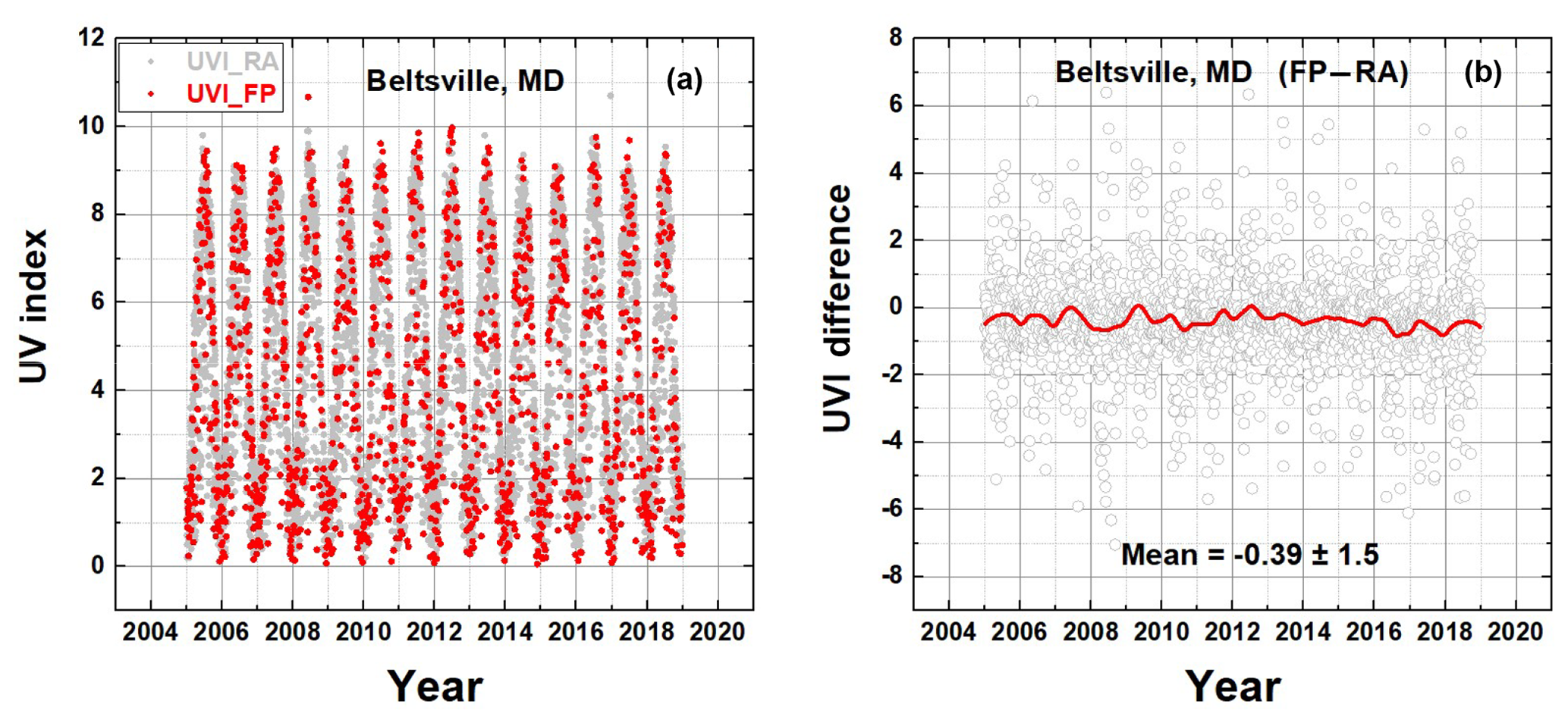
Figure 1 A comparison of the OMI erythemal irradiance algorithm (RA) with the fast polynomial algorithm (FP) for Beltsville, Maryland. (a) are the time series. (b) is the difference FP–RA. The red line is approximately a 1-year Loess(0.1) fit to the data.

Point-by-point comparison is difficult because of different temporal selection criteria where even small time differences produce rapid changes in E(t). To help with the comparison, the outputs from both algorithms are interpolated onto a common timescale (Figs. 1a and 2a). Differences are formed using the interpolated time series (Figs. 1b and 2). For Beltsville, Maryland (Fig. 1), with low absorbing aerosol amounts, the two algorithms agree to within a UVI mean of 0.39±1.5. A similar analysis is shown for four additional sites (Fig. 2). The OMI time series for RA (Fig. 1a) has many more points than for FP because of much stricter elimination of row-anomaly (Schenkeveld et al., 2017) points in the FP analysis. Approximately 1-year average Loess(0.1) fits to the difference data are shown. Loess(f) is a locally weighted least squares fit to a fraction f of the data points (Cleveland, 1981).

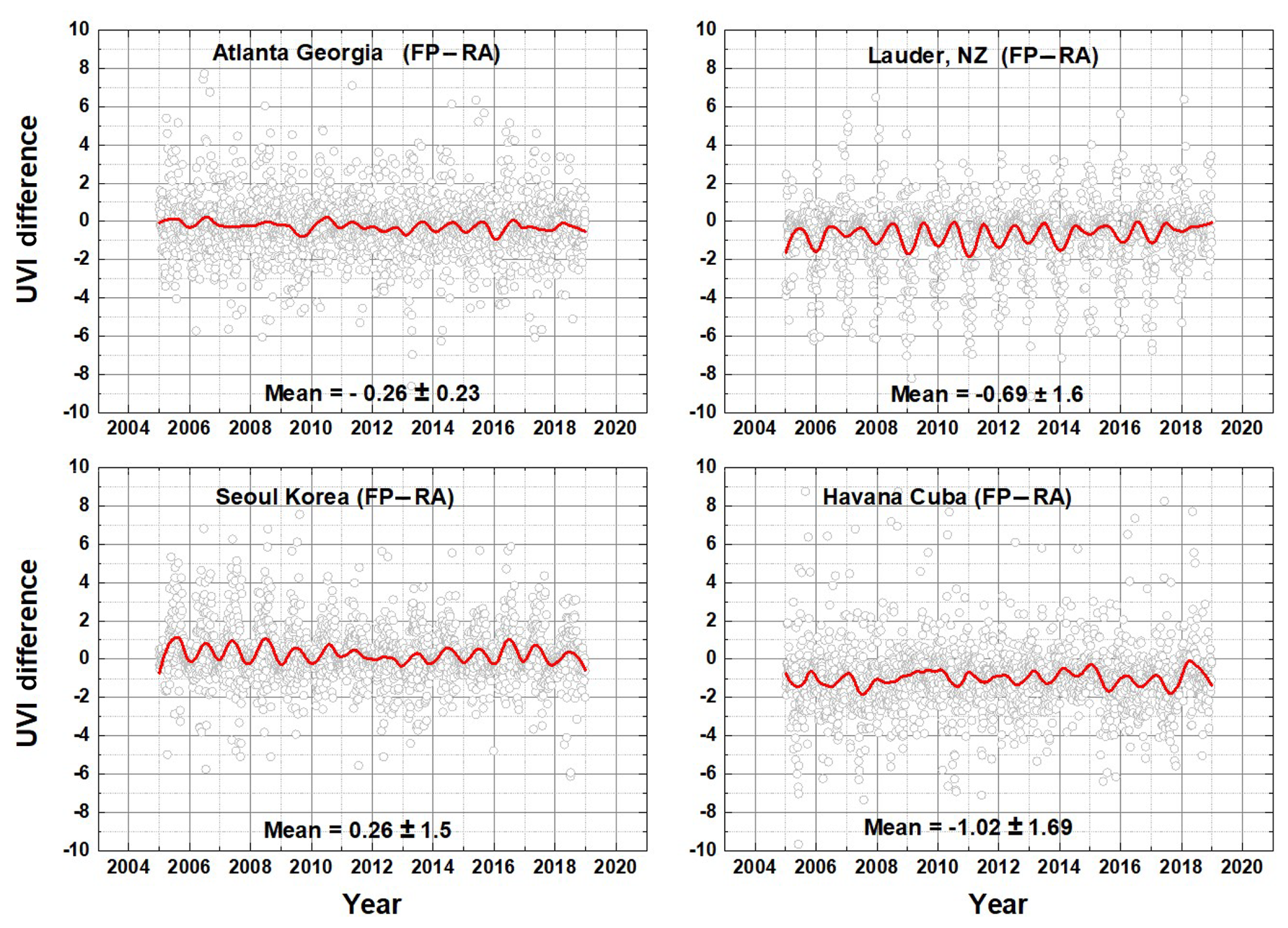
Figure 2 A comparison of the OMI erythemal irradiance algorithm (RA) with the fast polynomial algorithm (FP) for four sites. The red lines are approximately a 1-year Loess(0.1) fit to the data.

The site at Santiago, Chile, shows an overestimation case where the effect of absorbing and scattering aerosols may not be properly considered in calculations using OMI data for a city located in a depression surrounded by complex high terrain (Cabrera et al., 2012). Calculations in this paper (see Table A4) show a maximum summer value of UVI = 14, when ground-based measurements within the city show peak values near 12. The overestimate is consistent with calculations made previously using other satellite data (Cabrera et al., 2012). Another analysis of erythemal irradiance estimates from OMI satellite data in the New York City area (Fan et al., 2015) found that the calculated UVI overestimates the measured UVI under cloudy conditions, a result that might affect estimated trends.

2 Erythemal time series and LS linear trends

E(ζ, φ, z, t) is estimated using total column ozone amounts TCO₃ and 340 nm Lambert equivalent reflectivity LER, converted to transmission factors C_T (Krotkov et al., 2001; Herman et al., 2009).

$$\begin{array}{}\text{(4)}& C_{\mathrm{T}}(\mathit{\zeta },\mathit{\phi },z,t)=(\mathrm{1}-\mathrm{LER})/(\mathrm{1}-R_{\mathrm{G}}),(\mathrm{1}>C_{\mathrm{T}}>\mathrm{0}),\end{array}$$

where R_G is the spatially resolved 380–380 nm reflectivity of the Earth's surface (Herman and Celarier, 1997), with an average $<R_{\mathrm{G}}>$ of about 0.05, and aerosol absorption effects C_A(ζ, φ, z, t) that are retrieved from spectrally resolved irradiance measurements (300–550 nm) obtained from OMI for the entire Earth. OMI data are filtered to remove measurements obtained from portions of the CCD detector affected by pixels with a reduced sensitivity or “row anomaly” (Schenkeveld et al., 2017). OMI is a polar-orbiting side-viewing satellite instrument (2600 km width on the surface) onboard the AURA spacecraft that provides near-global coverage (nadir resolution field of view 13 km × 24 km) once per day from a 90 min polar orbit with an Equator-crossing time of approximately 13:30 local solar time (LST) (Levelt et al., 2018). Because of OMI's simultaneous side-viewing capability, there are occasionally second or third data points (±90 min) from adjacent orbits at higher-latitude locations.

This study uses TCO₃ (in Dobson units DU, 1 DU = 2.687×10¹⁶ molec cm⁻²) and 340 nm Lambert equivalent reflectivity LER (Herman et al., 2009) (LER is in reflectivity units, $\mathrm{0}<\text{RU}<\mathrm{100}$) data organized in gridded form for the entire sunlit Earth every 24 h. TCO₃ and LER data (2005–2018) at a resolution of $\mathrm{1}{}^{\circ }\times \mathrm{1}{}^{\circ }$ (https://avdc.gsfc.nasa.gov/pub/tmp/OMI_Daily_O3_and_LER/, last access: 16 June 2020) in ASCII format and ozone in HDF5 format from https://disc.gsfc.nasa.gov/datasets/OMTO3_V003/summary (last access: 16 June 2020) for latitude ζ, longitude φ, and time t, (in fractional years) were used to estimate noontime $E(\mathit{\zeta },\mathit{\phi },z,t)$. The LER data have been corrected for instrument drift (approximately 2 % in 14 years; see Fig. A6) by requiring that the LER values over the Antarctic high-plateau region remain constant over 14 years. The LER calibration correction permits 14-year LS trends to be estimated from Eq. (4). A gridded $\mathrm{1}{}^{\circ }\times \mathrm{1}{}^{\circ }$ Version 8.5 ozone product is available from https://avdc.gsfc.nasa.gov/pub/DSCOVR/OMI_Gridded_O3/ (last access: 16 June 2020). Site-specific time series are generated from the $\mathrm{1}{}^{\circ }\times \mathrm{1}{}^{\circ }$ degree latitude by longitude files. The numerical algorithm for erythemal analysis as applied for the Northern Hemisphere and Southern Hemisphere and the equatorial region is discussed in the Appendix. The same algorithm is applied to the synoptic sunrise to sunset data for the entire illuminated Earth obtained from EPIC for samples from the 2015–2019 period.

2.1 Multivariate linear regression model for calculating LS trends

Trends B(t) were determined for erythemal time series E(t) (similar for total column ozone and cloud transmission time series) using a generalized multivariate linear regression (MLR) model (e.g., Randel and Cobb, 1994, and references therein):

$$\begin{array}{}\text{(5)}& E\left(t\right)=A\left(t\right)+B\left(t\right)\cdot t+R\left(t\right),\end{array}$$

where t is the daily index (t =1 to 5113 for 2005–2018), A(t) is the seasonal cycle coefficient fit, B(t) is the linear LS trend coefficient fit, and R(t) is the residual error time series for the regression model. A(t) involves seven fixed constants, while B(t) is a single constant. The harmonic expansion for A(t) is

$$\begin{array}{}\text{(6)}& \begin{array}{rl}A\left(t\right)=& a\left(\mathrm{0}\right)+\sum _{p=\mathrm{1}}^{\mathrm{3}}\left[a\left(p\right)\cos (\mathrm{2}\mathit{\pi }pt/\mathrm{365})\right.\\ +& b\left(p\right)\sin (\mathrm{2}\mathit{\pi }pt/\mathrm{365})\left.\right],\end{array}\end{array}$$

where a(p) and b(p) are constants. Statistical uncertainties for A(t) and B(t) were derived from the calculated statistical covariance matrix involving the variances and cross-covariances of the constants (e.g., Guttman et al., 1982; Randel and Cobb, 1994). The linear deseasonalized trend results for various sites are listed in Tables 2–4 and A4 in percent per year with 1 standard deviation (1σ) uncertainty. For comparison of the trends and trend uncertainties derived from (5), trend analysis was also done using monthly average data (one data point per month). The trends and 1σ trend uncertainties derived from the monthly averages were found to be nearly identical to trends and 1σ uncertainties derived from the daily time-series data with gaps. The trends ΔE are expressed in % yr⁻¹ with $\mathrm{\Delta }\mathrm{E}=\mathrm{100}\mathrm{d}E/<E>$, where $<E>$ is the average value over the considered period.

Figure 3 (a) Erythemal irradiance $E(\mathit{\theta },\mathit{\phi },z,t)$ at six selected sites from Table A1 distributed within the United States. Listed are the 14-year UVI average maximum and average values (UVI = E∕25) (see Table 3). Mean and maximum values are 14-year averages. (b) Two sites from Fig. 1a, Greenbelt, Maryland, and Rural Georgia, with the effect of clouds and aerosols removed (i.e., T=1, τ_A=0).

2.2 Northern Hemisphere

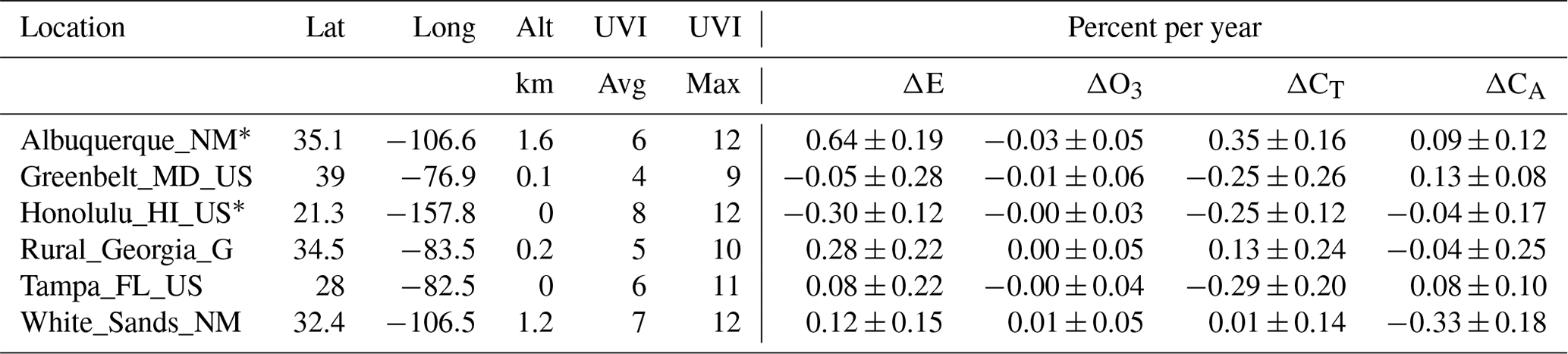
Figure 3 and Table 2 show erythemal irradiance $E(\mathit{\zeta },\mathit{\phi },z,t)$ time series (mW m⁻²) and their LS linear trends (in percent change per year along with their 1σ standard deviation) at six sites with various altitudes z within the United States from 2005 to 2018 (14 annual cycles). The right-hand side axis shows the proportional values of the standard UV index, UVI = E ∕ (25 mW m⁻²). Erythemal time series are truncated to start and stop at the same point in their 14-year annual cycles (1 January 2015 to 31 December 2018).

The time series depicted in Fig. 3 are non-uniform in time, with gaps, mostly from the row anomaly, between some adjacent points. In all cases the gaps are small enough to properly represent the SZA dependence of the erythemal irradiance. Of the six United States sites listed in Table 2, Albuquerque, NM, and Honolulu, HI, have trends, $\mathrm{\Delta }\mathrm{E}=\mathrm{100}\mathrm{d}E/<E>$, with better than 2-σ standard deviations 0.64±0.19 % yr⁻¹ and $-\mathrm{0.30}\pm \mathrm{0.12}$ % yr⁻¹, respectively. These sites have small changes in TCO₃ ($-\mathrm{0.03}\pm \mathrm{0.05}$ % yr⁻¹ and $-\mathrm{0.00}\pm \mathrm{0.03}$ % yr⁻¹) but significant changes in cloud + haze transmission C_T, 0.35±0.16 % yr⁻¹ and $-\mathrm{0.25}\pm \mathrm{0.12}$ % yr⁻¹, and absorbing aerosol transmission (0.09±0.12 % yr⁻¹ and $-\mathrm{0.04}\pm \mathrm{0.17}$ % yr⁻¹), respectively (see Table 2).

Of human health interest are the maximum values that occur during the summer months when the solar zenith angle is near a local minimum reducing the slant column ozone absorption and Rayleigh scattering for clear-sky days. In terms of the UV index, a value of 6 will produce significant skin reddening in light-skinned people in about an hour of unprotected exposure (Diffey, 1987, 2018; Italia and Rehfuess, 2012). In local shade, there is reduced but significant exposure from atmospheric scattering (Herman et al., 1999), with shorter more damaging wavelengths scattering the most. For three low-latitude US sites in Table 2, the 14-year average maximum UVI reaches 12, with Tampa, FL, reaching 11. For sites with extremely high UVI (10–18), even shaded areas can produce damaging exposure from scattered UV. Table 2 shows the 14-year average maximum UVI and the 14-year average UVI.

Table 2 Trends for locations in the United States (errors are 1σ).

^∗ Means 2-σ trend significance for erythemal change.

For the mid-latitude site, Greenbelt, MD, at 39^∘ N, summer values between 8 and 9 are frequently reached, with a few days reaching 10 and 1 d reaching 11 on 6 June 2008. The cause of UVI = 11 was a low ozone value of 283 DU on a clear-sky day compared to more normal values between 310 and 340 DU. The basic annual cycle follows the SZA, with the minimum angle and maximum E occurring during the summer solstice. For Greenbelt, MD, this angle is approximately 39–23.45^∘ = 15.55^∘. Sites with fewer clouds plus haze and closer to the Equator have higher maximum UV-index values, 12 for White Sands, NM, and 11 for Tampa, FL. Trend results corresponding to Fig. 3a are summarized in Table 2 and Appendix Table A4. The last four columns give the estimated LS trend B(t) from Eq. (4) for each time series and the standard deviation 1σ. Graphs summarizing the more extensive Table A4 are given in Sect. 2.5, which show the expected change in UVI for a wide range of locations at various latitudes. Since the purpose is estimating changes in E from all causes, the effects of the quasi-biennial oscillation (QBO), ENSO (El Niño–Southern Oscillation), and the 11-year solar cycle are not removed from the ozone time series. Figure 3b shows the increases in erythemal irradiance for Greenbelt (UVI = 11) and Rural Georgia (UVI = 12) when the effects of clouds and aerosols are removed from the calculations.

When θ(t) = SZA, C_A(t), and C_T(t) (transmission) are held constant for calculating E(θ(t), O₃(t), C_T(t), and C_A(t)), a 1 % change in total column ozone amount Ω = TCO₃ produces approximately a 1.2 % change ΔE in erythemal irradiance. The exact amount of change is dependent on the SZA selected (Eq. 6). The values for ΔO₃, ΔC_A, and ΔC_T change (% yr⁻¹) are given in Table 2, which shows that a significant amount of the erythemal irradiance change over 14 years is caused by changes in cloud cover except for White Sands, NM.

A numerical solution of the radiative transfer equation for the erythemal action spectrum can be approximated by a power-law form as a function of θ = SZA and Ω = TCO₃ (Eq. 6 and Appendix Eq. A4), where the cloud and aerosol transmission are given by C_T and C_A. This form gives an improved version of the radiation amplification factor (Madronich, 1995) R(θ) that is independent of TCO₃ (Herman, 2010). With cloud and aerosol absorption represented by C_T and C_A factors, 0<C_T or C_A<1.

$$\begin{array}{}\text{(7)}& E(\mathrm{\Omega },\mathit{\theta })=U\left(\mathit{\theta }\right)(\mathrm{\Omega }/\mathrm{200}{)}^{-R\left(\mathit{\theta }\right)}{C}_{\mathrm{T}}{C}_{\mathrm{A}}\end{array}$$

For a given time, t, the sensitivities of E to changes in Ω, θ, C_T, and C_A are

$$\begin{array}{}\text{(8)}& \begin{array}{rl}{\displaystyle \frac{\mathrm{d}E}{E}}=-& R\left(\mathit{\theta }\right){\displaystyle \frac{\mathrm{d}\mathrm{\Omega }}{\mathrm{\Omega }}}+{\displaystyle \frac{\mathrm{d}{C}_{\mathrm{T}}}{C_{\mathrm{T}}}}+{\displaystyle \frac{\mathrm{d}U\left(\mathit{\theta }\right)}{U\left(\mathit{\theta }\right)}}\\ -& R\left(\mathit{\theta }\right)\ln \left({\displaystyle \frac{\mathrm{\Omega }}{\mathrm{200}}}\right){\displaystyle \frac{\mathrm{d}R\left(\mathit{\theta }\right)}{R\left(\mathit{\theta }\right)}}+{\displaystyle \frac{\mathrm{d}{C}_{\mathrm{A}}}{C_{\mathrm{A}}}},\end{array}\end{array}$$

where, for example, d$U\left(\mathit{\theta }\right)=U(\mathit{\theta }+\mathrm{d}\mathit{\theta })-U\left(\mathit{\theta }\right)$ and d$R\left(\mathit{\theta }\right)=R(\mathit{\theta }+\mathrm{d}\mathit{\theta })-R\left(\mathit{\theta }\right)$.

For θ=0, R(0)=1.2 and R(θ) gradually decrease to 0.85 for $\mathit{\theta }=\mathrm{80}{}^{\circ }$ (Herman, 2010, and Appendix Fig. A1). SZA variation is the primary anti-correlated driver for the annual cycle of erythemal irradiance (Fig. 3) at each location, except when there is heavy cloud cover. The cycle for $E(\mathit{\theta },\mathit{\phi },z,t)$ is perturbed by the smaller effect of short-term changes in Ω,C_T, and C_A that are shifted in phase from θ(t). The result is that the separately estimated 14-year linear trends for C_T and Ω are not necessarily additive when using Eqs. (4) and (5). For example, for the Albuquerque, NM, site (Fig. 3), the erythemal trend is statistically significant at 0.64±0.19 % yr⁻¹. Contributing factors are the cloud transmission function C_T trend $\mathrm{\Delta }{\mathrm{C}}_{\mathrm{T}}=\mathrm{0.35}\pm \mathrm{0.16}$ % yr⁻¹ (positive means more transmission), aerosol absorption function C_A trend Δ $C_{\mathrm{A}}=\mathrm{0.09}\pm \mathrm{0.12}$ % yr⁻¹, and small Ω(t) trend $\mathrm{\Delta }\mathrm{\Omega }=-\mathrm{0.03}\pm \mathrm{0.05}$ % yr⁻¹. The ΔE trend for Albuquerque without cloud reflectivity and aerosol absorption is 0.04±0.3 % yr⁻¹, corresponding to the small change in just ozone, $\mathrm{\Delta }{\mathrm{O}}_{\mathrm{3}}=-\mathrm{0.03}\pm \mathrm{0.05}$.

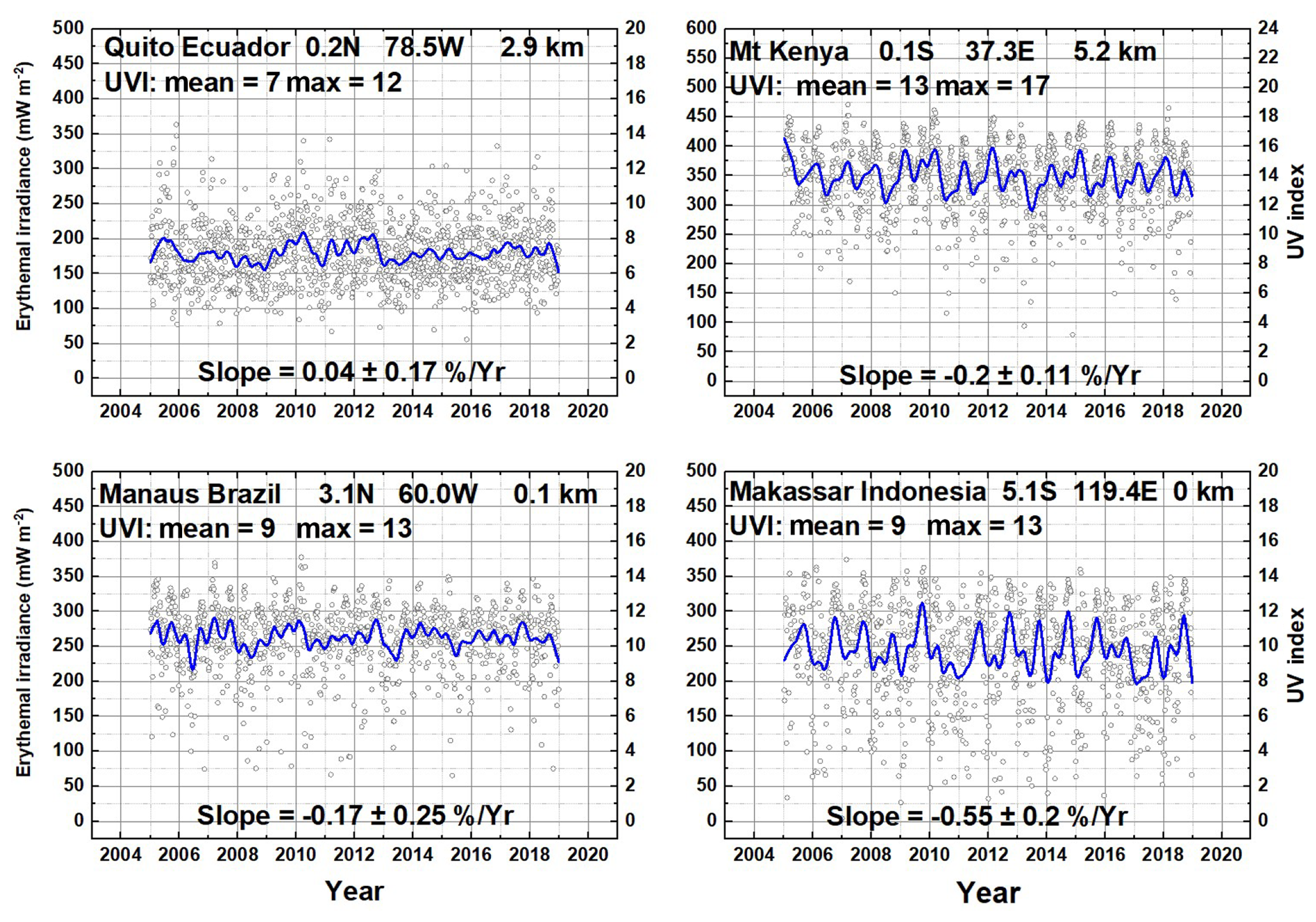
Figure 4 Four sites located close to the Equator. Mt. Kenya at 0.1^∘ S, Quito, Ecuador at 0.2^∘ N, Makassar, Indonesia at 5.1^∘ S, and Manaus, Brazil at 3.1^∘ N. The blue lines are a Loess(0.04) fit (approximately 6-month LS running average). Mean and maximum values are 14-year averages. Slope = B in Eq. (5).

2.3 Equatorial region

The equatorial region is unique for erythemal irradiance, since TCO₃ is a minimum and the SZA has a twice-yearly minimum as the solar declination angle changes between $\pm \mathrm{23.45}{}^{\circ }$. Four selected equatorial sites (Fig. 4 and Table 3) show very different behavior compared to mid-latitude sites (Fig. 3 and Table 2).

Equatorial sites listed in Table A4 have very high UVI maximum values (e.g., Darwin, AU 12.5^∘ S, 0 km, UVIM = 14; Lima, PE, 12^∘ S, 0.2 km, UVIM = 15; Kinshasa,CD, 4.3^∘ S, 0.3 km, UVIM = 14; Nairobi, 1.1^∘ N KE, 1.9 km, UVIM = 15; Bogota, CO, 4.6^∘ N, 2.5 km, UVIM = 15) with a significant number of clear-sky days. There are exceptions where there is considerable cloud cover on many days, such as Manaus, Brazil, and Quito, Ecuador. The average E(ζ, φ, z) is higher (mean $<\text{UVI}>=\mathrm{9}$, UVIM = 14) for the near-sea-level site in Manaus, Brazil (1.8 million people), than the equally populated city of Quito, Ecuador (1.85 million) at 2.9 km altitude (mean $<\text{UVI}>=\mathrm{7}$, UVIM = 12). The lower average Quito value is caused by the presence of additional cloud cover (mean transmission <C_T>=0.34) compared to Manaus (mean transmission <C_T>=0.68) even though the Quito altitude is considerably higher. The effect of high altitude, 5.2 km with relatively clear skies, is seen for the Mt. Kenya site at 0.1^∘ S with UVIM = 18.

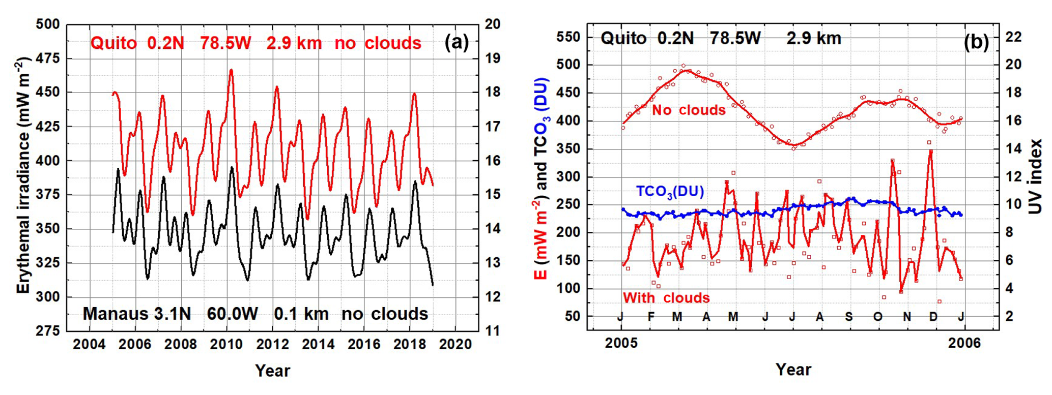
Figure 5 (a) A 2-week running average of cloud-free $E(\mathit{\zeta },\mathit{\phi },z,t)$ corresponding to the data in Fig. 3a for Quito, Ecuador, and Manaus, Brazil, showing the effect of height and a small difference in average ozone amount. (b) An temporal expansion for 1 year (2005) of $E(\mathit{\zeta },\mathit{\phi },z,t)$ estimates for Quito showing the double peak as a function of minimum SZA near the equinoxes in the absence of clouds that is masked when clouds are included. The blue line shows the 20 DU variation in ozone between March and September. Solid lines in panel (a) are an Akima spline fit.

Figure 5a shows the effect of altitude causing an increase in clear-sky $E(\mathit{\zeta },\mathit{\phi },z,t)$ for Quito (2.9 km) compared to Manuas (0.1 km) plus a small difference in average TCO₃ (2 %) between the two locations. Without clouds, Fig. 5, both sites show a double peak corresponding to SZA = 0^∘ twice a year near the March and September equinoxes. Figure 5b has an expanded timescale for 2005 showing the double peak for Quito and the strong effect of clouds in the region. The 14-year average cloud-free value for Quito is <UVI>=16 and a maximum UVI = 19. The minimum cloud-free value is <UVI>=15 instead of 3 when cloud cover is included. Compared to Quito, the cloud effect is less at the Manaus, Brazil, and Mt. Kenya sites, and even at the coastal Makassar, Indonesia site. The 20 DU variation in TCO₃ causes the autumn peak in $E(\mathit{\zeta },\mathit{\phi },z,t)$ without clouds to be smaller than the spring peak. Note that there are only 90 points in 2005 because of data gaps in OMI equatorial data and the effect of losing points because of the row anomaly.

The calculations based on $\mathrm{1}{}^{\circ }\times \mathrm{1}{}^{\circ }$ (100×100 km²) spatial resolution can obscure an important health-related result. In Quito, there are frequent localized clear periods when the UV index can rise to the clear-sky values (13 < UVI < 18), an increase of about 10, which is a serious health threat for skin cancer and cataracts all year. At all sites, ground-based measurements show that UV irradiance at the ground can briefly exceed the clear-sky value because of reflections from nearby clouds (Sabburg and Wong, 2000). In Honolulu (21.3^∘), the double peaks in $E(\mathit{\zeta },\mathit{\phi },z,t)$ are not significantly separated in time (15 d) to be easily discernable, but it causes the slightly different shape in the annual cycle (Fig. 3a). In general, equatorial sites have increased $E(\mathit{\zeta },\mathit{\phi },z,t)$ compared to higher latitudes because of both lower SZA values and less ozone near the Equator, giving reduced UV absorption and increased $E(\mathit{\zeta },\mathit{\phi },z,t)$.

Table 3 Summary of four equatorial sites (errors are 1σ).

^∗ Means 2-σ trend significance for erythemal change.

Two of the four equatorial sites in Fig. 4 and Table 3 show significant linear trends B(t) (Makassar, Indonesia, and Mt. Kenya, Kenya), with the Makassar, Indonesia, site showing the largest linear trend, $-\mathrm{0.55}\pm \mathrm{0.2}$ % yr⁻¹. For Makassar, ozone is increasing at a rate of 0.17±0.02 % yr⁻¹, which by itself would cause UVI to decrease at a rate of $-\mathrm{0.20}\pm \mathrm{0.01}$ % yr⁻¹. Atmospheric transmission (Table 3) is decreasing at a rate of $-\mathrm{0.16}\pm \mathrm{0.19}$ % yr⁻¹, causing $E(\mathit{\zeta },\mathit{\phi },z,t)$ to have a net decrease. In the absence of clouds, the percent decrease in ozone amount causes an increase in $E(\mathit{\zeta },\mathit{\phi },z,t)$ at approximately a 1.2:1 ratio. Figure 5a shows the approximate anti-correlation between ozone amounts and $E(\mathit{\zeta },\mathit{\phi },z,t)$ for Quito and Manaus. This is modified by the 6-month shifting of the sub-solar point (SZA = 0). When all four periodic and quasi-periodic effects are combined, the result is the aperiodic function shown in Fig. 5b for Quito, Ecuador. Similar analysis applies for Manaus, Brazil, located near the Amazon River, which is dominated by variable cloud-driven atmospheric transmission, but less than for Quito, Ecuador. The other two equatorial sites Makassar, Indonesia, and Mt. Kenya, Kenya have smaller cloud effects and show periodic structures driven by SZA and ozone absorption.

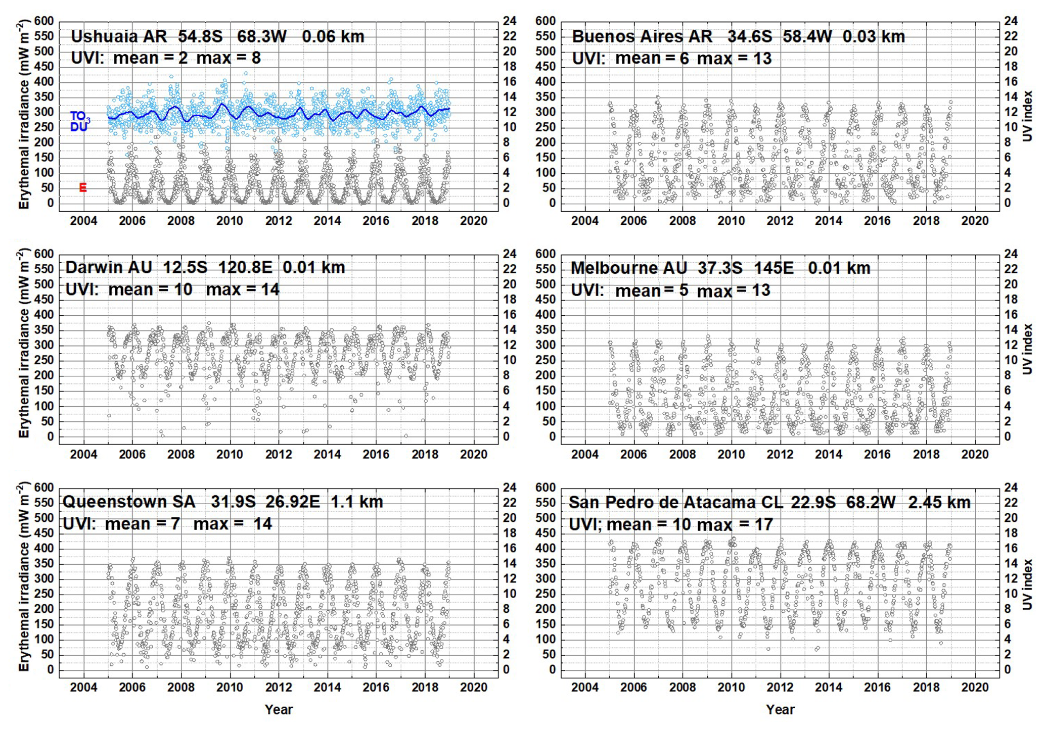
Figure 6 Six sites in the Southern Hemisphere including estimates of the trends for $E(\mathit{\zeta },\mathit{\phi },z,t)$, TCO₃, and the atmospheric transmission C_T caused by clouds and haze. The TCO₃ time series (blue) is shown for Ushuaia.

2.4 Southern Hemisphere

Time series for the Southern Hemisphere are represented by six sites shown in Fig. 6 ranging in latitude and altitude (12.5 to 54.8^∘ and 0 to 2.5 km). The maxima occur close to the December solstice date, with the exact date shifted by cloud cover, and the minima occur near the June solstice date. Of these, Darwin, Australia, is within the equatorial zone (12.5^∘ S) and shows the double-peak structure with peaks separated by about 85 d. The site furthest from the Equator, Ushuaia (54.8^∘ S), has the lowest UVI peak value of 9.6 (14-year average maximum UVI = 8) and the lowest 14-year minimum average UVI = 2. Occasionally the Antarctic ozone depletion region passes over Ushuaia, giving rise to increased UV amounts, but these episodes (September–October) usually do not correspond to the maximum UVI values that occur with the minimum SZA in January. The 20-year historical ground-based measurement record at Ushuaia starting in 1988 (Bernhard et al., 2010) shows higher values, 11.5, when the Antarctic ozone hole moved overhead in October, even though the SZA is not a minimum.

For the sites in Fig. 6, the populated sites San Pedro de Atacama, CL, and La Quiaca, AR, have the largest UVI maximum (17 and 18) and average (11), since they are at significantly higher altitudes (2.5 and 4.5 km) and are located at the southern edge of the equatorial zone (23 and 22^∘ S) with a relatively clear cloud-free atmosphere. More than half of the days each year have 10 < UVI < 18. This 14-year average UVIM is higher than for equatorial Darwin, Australia, UVI < 15.5. The frequent June minima for Darwin are UVI = 8, with occasional days at UVI = 2 caused by clouds, while the almost cloud-free San Pedro de Atacama has minima of UVI = 4 corresponding to a June noon SZA = 46^∘ compared to Darwin June SZA = 36^∘. Both sites have about the same typical TCO₃, 255 DU.

Table 4 Summary for seven Southern Hemisphere sites (errors are 1σ).

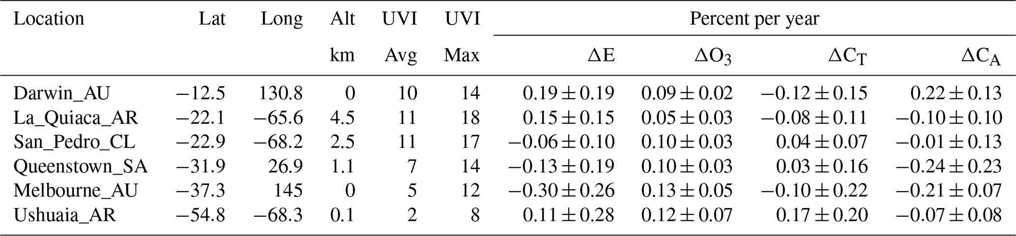
Previous estimations of erythemal irradiance from ground-based measurements (1997–1999) and calculations (using Total Ozone Mapping Spectrometer data) at Ushuaia (Cede et al., 2002, 2004) show very similar values, with UVI < 1 in the winter (June) and with 14-year average maximum values up to 8. The OMI data show an occasional day reaching UVI = 10 during the summer (December–January). Buenos Aires at lower southern latitudes has values of UVI from 1 to 2 in the winter and up to 12–13 in the summer. These values approximately agree with those in Table 4. Cede et al. (2004) give ground-based results for eight sites that also include a higher-altitude equatorial site, La Quiaca, AR (22.1^∘ S), at 3.46 km altitude, with very high summer values up to UVI = 20. The corresponding calculated estimates using OMI data (2005–2018) also have the maximum UVI = 20 occurring in 2010 with a 14-year average maximum of UVIM = 18 (Table 4). None of the ΔE in Table 4 are statistically significant at 2σ.

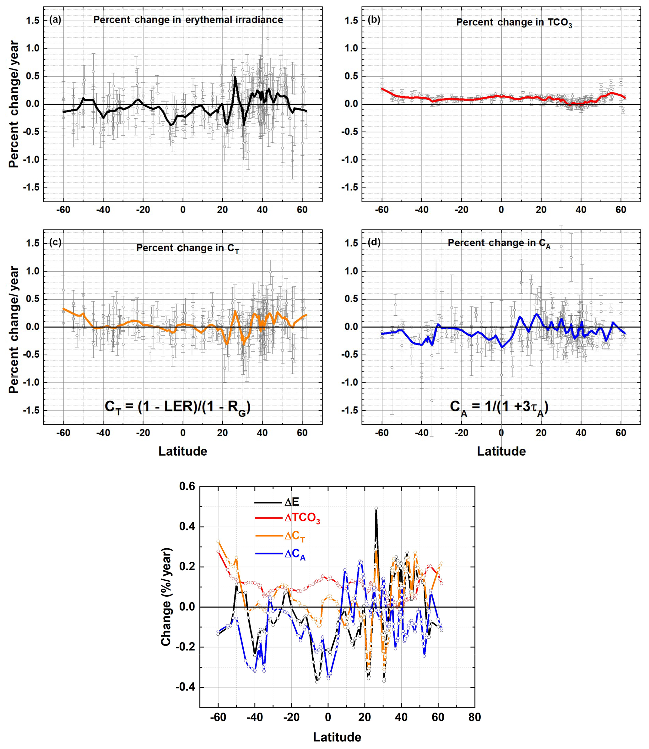
Figure 7 (a) Percent change per year for (a) erythemal irradiance ΔE, (b) ΔTCO₃ (total column ozone) for the period 2005–2018, (c) ΔC_T (atmospheric transmission), and (d) ΔC_A (absorbing aerosol transmission) from OMI observations at individual sites (see Table A4). The solar cycle and quasi-biennial oscillation effects have not been removed. Error bars are 1σ. Solid curves are Loess(0.1) fits to the data (15^∘ averaging) and are shown in Fig. 7b with the same color code. A geographic map of the land locations in Table A4 and Fig. 7 is shown in Fig. A3. (b) Loess(0.1) fits from Fig. 7a showing the correlation of ΔE with ΔC_A and ΔC_T and anticorrelation with ΔTCO₃.

2.5 Trends ΔE, ΔΩ, ΔC_T, and ΔC_A vs. latitude

Figure 7 shows the 14-year LS trends (Eq. 4) (% yr⁻¹) ΔE, ΔΩ, ΔC_T, and ΔC_A and the 1σ error estimate for land (Table A4 and Fig. A3) plus Atlantic and Pacific Ocean sites distributed in latitude from 60^∘ S to 60^∘ N. The colored solid lines are a Loess(0.1) fit to the trend data that is approximately equivalent to a 15^∘ latitude running average with least squares weighting. Figure 8 contains the same Loess(0.1) fits on an expanded common scale. The 1σ error estimates are large enough to conclude that there are few significant changes in E at the 2-σ confidence level for many of the individual sites (see sites prefaced with ^∗ in Table A4). However, the Loess(0.1) curves show significant correlation with each other, suggesting that the increases and decreases from combining sites within a 15^∘ latitude band are significant and not just noise.

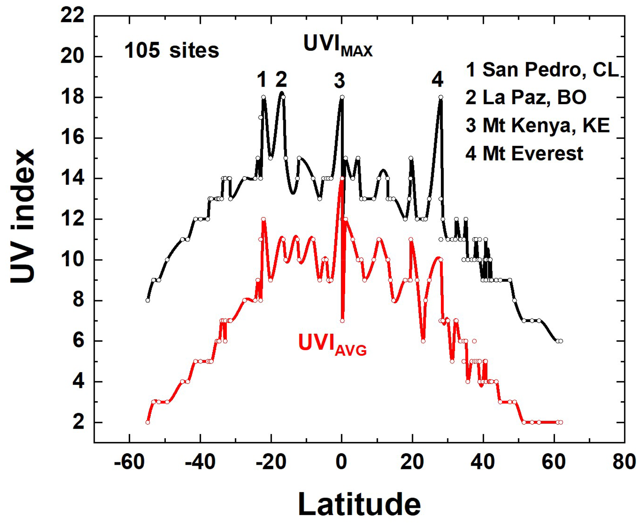
Figure 8 Fourteen-year UVI average and UVI maximum from Table A4 for 105 sites. Solid curves are Akima spline fits (Akima, 1970) to the individual site data points. There are four high-altitude sites listed: San Pedro, Chile (2.45 km), La Paz, Bolivia (3.78 km), Mt. Kenya, Kenya (5.2 km), and Mt. Everest, Nepal and China (8.85 km).

For the UV portion of the spectrum represented by the erythemal irradiance action spectrum, the ΔE is affected by changes in TCO₃ that change relatively slowly with latitude (Fig. 7a, b). ΔTCO₃ drives changes (1±0.5 % per decade 40^∘ S to 30^∘ N, 0.3±0.3 % per decade 25 to 45^∘ N, 1.4±0.6 % per decade 45 to 60^∘ N). The ozone changes (Fig. 7b) obtained from OMI observations include the effects of the 11.3-year solar cycle, the quasi-biennial oscillation QBO, and the El Niño–Southern Oscillation (ENSO) effects, and, as such, are not the standard ozone trend amounts (Weber et al., 2017; WMO, 2018). There are significant increases of 1.1±1.2 % per decade in ΔC_T at high southern latitudes (mostly cloud reflectivity) for a latitude range, 60 to 45^∘ S (Fig. 7c) with a significant decrease around 22 and 35^∘ N and an increase near 22.5^∘ N.

Atmospheric transmission C_T increased (cloud reflectivity decreased) by 1±0.9 % per decade for 35 to 60^∘ N for the period 2005 to 2018, implying that solar insolation has also increased for all UV (305–400 nm), visible (400–700 nm), and near-infrared wavelengths (700–2000 nm). Atmospheric transmission in the presence of absorbing aerosols C_A has decreased in the equatorial zone by $-\mathrm{1.9}\pm \mathrm{0.9}$ % per decade for 20^∘ S to 5^∘ N (panel d) and at southern latitudes by $-\mathrm{1.8}\pm \mathrm{1.3}$ % per decade for 60 to 30^∘ S. C_A in the Northern Hemisphere shows two peaks centered on 5 and 18^∘ N and oscillates about zero $-\mathrm{0.1}\pm \mathrm{1}$ % per decade for 5 to 60^∘ N. ΔE is correlated with changes in cloud transmission ΔC_T and absorbing aerosols associated with cities ΔC_A (Fig. 7b). Since ΔTCO₃ changes slowly with latitude compared to ΔC_T and ΔC_A, the effect of ΔTCO₃ is more of an offset compared to the stronger latitudinal variation effect of aerosols and clouds.

Figures 7a, b, and 8 are limited to $\pm \mathrm{60}{}^{\circ }$ latitude, since estimating $E(\mathit{\zeta },\mathit{\phi },z,t)$ over the Arctic or Antarctica snow and ice from OMI data is likely not accurate because the LER of the scene is approximately treated as if there were a cloud instead of a bright surface. In Antarctica's Palmer Peninsula, the annual erythemal irradiance cycle ranges from 0 in winter (May to August) to a variable maximum in the spring and summer months depending on the year. For example, estimates from OMI data with C_T=1 (clear sky) are 125 mW m⁻² (UVI = 5) in 2013 and 175 mW m⁻² (UVI = 7) in 2016. The year-to-year variation in the maximum E(ζ, φ, z, t) is driven by the highly variable Antarctic TCO₃ hole.

Figure 8 shows a latitudinal plot of the maximum and average UVI over 14 years from 105 of the land sites listed in Appendix Table A4. The maximum values over 14 years show the high summertime UVI levels that can be expected at individual sites, especially for the four indicated high-altitude sites. The maximum summer values at all latitudes between 60^∘ S and 60^∘ N exceed UVI = 6, which is considered high enough to cause sunburn for unprotected skin (Sánchez-Pérez et al., 2019) in 20 to 50 min depending on skin type. Higher values of UVI can produce sunburn in much shorter times. For example, for UVI = 10, sunburn can be produced in as little as 15 min for Type 1 and Type 2 skin (Caucasian and Asian) to 30 min unprotected exposure for Type 4 skin (Sanchez-Perez, 2019).

The highest UVI values in Table A4 and Fig. 8 are associated with four high-altitude sites. Two of these are populated cities, San Pedro de Atacama (2.5 km, population = 11 000), Chile, and La Paz, Bolivia (3.8 km, population = 790 000). These two high-altitude sites have very high UVI associated with their low latitudes and relative lack of clouds on some days. Over the 14 years of this study, the UVI at San Pedro de Atacama has remained approximately constant ($-\mathrm{0.06}\pm \mathrm{0.10}$ % yr⁻¹), while at La Paz, Bolivia, the UVI has decreased at a rate of $-\mathrm{0.59}\pm \mathrm{0.16}$ % yr⁻¹ caused by an increase in ozone amount (0.1±0.02 % yr⁻¹), a decrease in atmospheric transmission C_T from increasing cloud cover ($-\mathrm{0.48}\pm \mathrm{0.14}$ % yr⁻¹), and a decrease in absorbing aerosol transmission C_A ($-\mathrm{0.24}\pm \mathrm{0.13}$ % yr⁻¹) from increasing amounts of absorbing aerosols. The height dependence of UVI for Mt. Everest (8.8 km) is linearly extrapolated from calculations for 0 to 5 km (Eq. A4 and Table A3). Radiative transfer calculations of the height dependence to 8 km show that this is a good approximation.

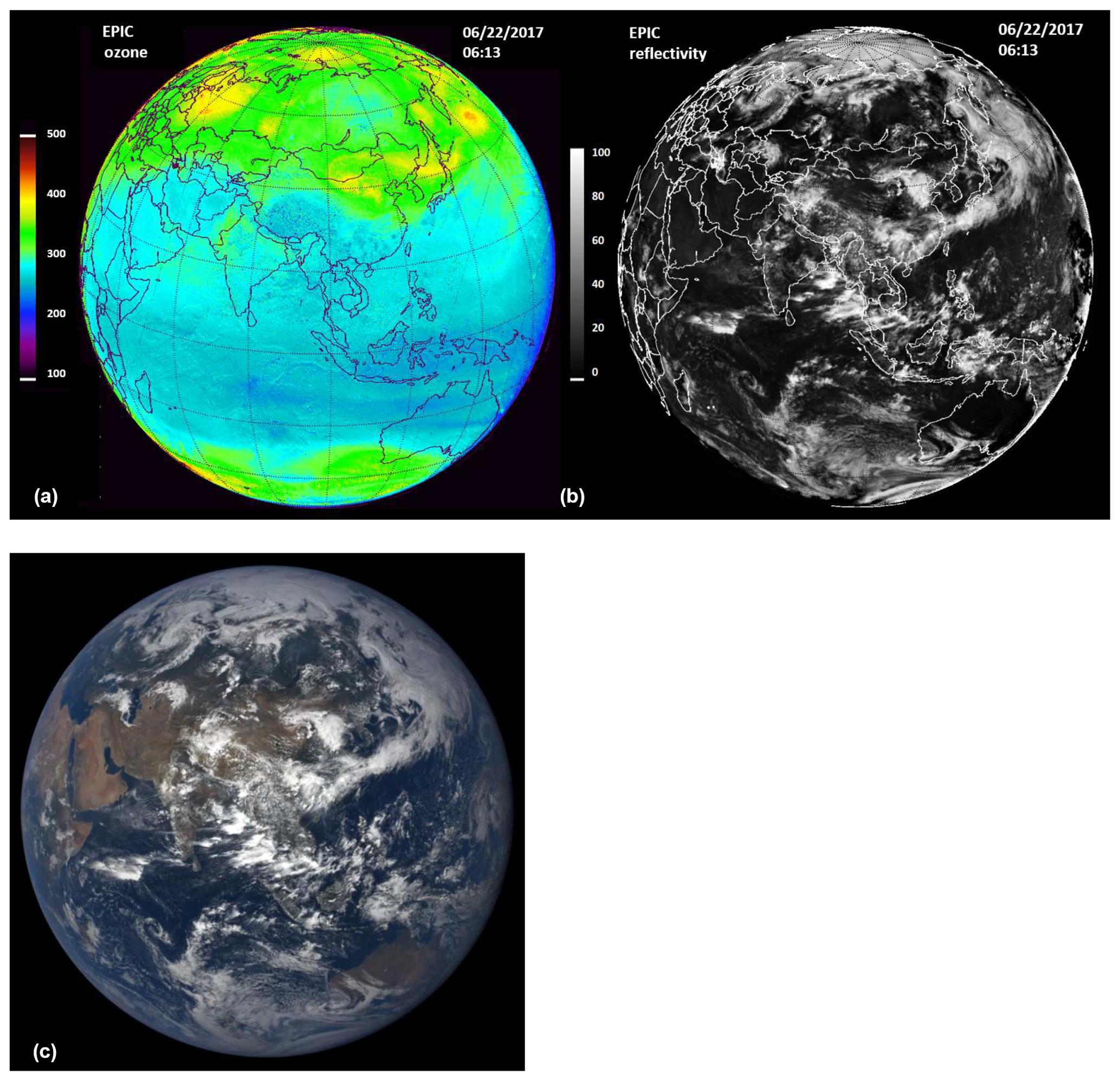
Figure 9 EPIC-derived TCO₃ (upper left in DU: 100 to 500 DU) and reflectivity (LER upper right in percent or RU: 0 to 100) for 22 June 2017 at t_O=06:13 GMT. Lower left: color image of the Earth showing clouds and land areas. The brighter clouds are optically thick and correspond to the higher values of the LER. Figure map created with IDL^®. Color image available at https://epic.gsfc.nasa.gov/ (last access: 16 June 2020).

3 Global view of E(ζ, φ, t_O) of sunrise to sunset distributions from DSCOVR EPIC

EPIC onboard the DSCOVR spacecraft views the sunlit disk of the Earth from a small orbit about the Earth–Sun gravitational balance point (Lagrange-1 or L₁) 1.5 million km from the Earth. EPIC has 10 narrow-band filters ranging from the UV at 310 nm to the near infrared, 870 nm that enable measurements of TCO₃ and LER with 18 km nadir resolution using a 2048×2048-pixel charge-coupled detector. EPIC takes multiples (12 sets in October–March to 22 sets in April–September) of 10 wavelength images per day as the Earth rotates on its axis. The instrumental details and calibration coefficients for EPIC are given in Herman et al. (2018) as well as some examples of UV estimates.

EPIC-estimated UV irradiances reaching the Earth's surface are derived from measured TCO₃ and 388 nm LER for about 3 million grid points as shown for 22 June 2017 at $t_{\mathrm{O}}=\mathrm{06}:\mathrm{13}$ GMT (Fig. 9). The relative accuracy of clear-sky EPIC-calculated E compared to that from OMI is derived from the relative accuracy of TCO₃ measurements, computing the global and seasonal average E percent difference $\mathrm{100}(E_{\mathrm{EPIC}}-E_{\mathrm{OMI}})/E_{\mathrm{EPIC}}=\mathrm{1.4}\pm \mathrm{1}$ %. In the presence of clouds, local differences may be larger, since the OMI latitudinal overpass GMT can vary by ±20 min from the Equator-crossing GMT, causing apparent changes in local cloud cover from the specific EPIC GMT t_O. Also, the OMI analysis contains an assumption that TCO₃ C_A and C_T measured at $\mathrm{13}:\mathrm{30}\pm \mathrm{00}:\mathrm{20}$ apply to the local noon erythemal calculation (SZA = latitude–solar declination). TCO₃, C_A, C_T, and terrain height maps z are converted into E(ζ, φ, z, and t_O) for each grid point at the specified GMT time t_O using the algorithm given in the Appendix. As with OMI, R = LER is converted into cloud transmission C_T using $C_{\mathrm{T}}=(\mathrm{1}-R)/(\mathrm{1}-R_{\mathrm{G}})$. The quantitative LER map in Fig. 9 can be compared to the color image of the Earth obtained by EPIC (also Fig. 9), where the high values of LER correspond to the high bright white clouds shown in the color image. Ozone absorption mostly affects the short wavelength portion of the erythemal spectrum (300–320 nm), with only negligible absorption from 340 to 400 nm. The results, including the effects of TCO₃, LER and Rayleigh scattering to estimate erythemal irradiance, are shown in Fig. 10 (upper left) for 22 June 2017 with t_O=06:13 GMT.

Figure 10 Erythemal irradiance $E(\mathit{\zeta },\mathit{\phi },z,t)$ and UVI($\mathit{\zeta },\mathit{\phi },z,t$) from sunrise to sunset for the 21 June 2017 solstice. The three images are for different GMT. (a) 22 June 2017 (06:13 GMT). (b) 21 June 2017 (11:21 GMT) and (c) 21 June 2017 (19:00 GMT). The images correspond to the sub-solar points over different continents caused by the Earth's rotation (15^∘ h⁻¹). Figure map created with IDL^®.

The data from each EPIC image are synoptic (same GMT), so that the ozone, reflectivity, and erythemal results are from sunrise (west or left) to sunset (right or east) with decreasing E for SZA near sunrise and sunset. A similar erythemal darkening effect from increased SZA occurs for northern and southern higher latitudes. In these images, local solar noon is near the center of the image but offset by EPIC's orbital viewing angle that is always 4 to 15^∘ away from the Earth–Sun line. In the case shown, the 6-month orbit is offset about 10^∘ to the west. Three months earlier in March and 3 months later in September, the orbit is offset to the east.

Erythemal maps in subsequent figures are organized by season (December and June solstices and March and September equinoxes). The maximum values of E(ζ, φ, t_O) follow the minimum SZA modified by cloud amount. Since the sub-solar point moves north and south with the annual change in the Earth's declination angle (between ±23.45^∘), the maximum clear-sky UVI usually occurs near local solar noon (LST) with the smallest SZA. An exception is when the effect of increased altitude is larger than the SZA effect.

3.1 Northern Hemisphere summer solstice (June)

For the June solstice view (Fig. 10), the EPIC view includes the entire Arctic region and areas to about 55^∘ S. The center longitude of the image is close to local solar noon. The view is with north up and from sunrise (west or left) to sunset (east or right). The effect of the orbital distance from the Earth–Sun line can be seen in the asymmetry of the near-sunrise and sunset regions, implying that the 6-month orbit was off to the southwest of the Earth–Sun line. The images were selected to give estimates of erythemal irradiance over Asia, Africa, and the Americas as a function of latitude, altitude, and longitude (time of the day) for a specific Greenwich Mean Time (GMT) for each map.

In Fig. 10 high UVI is seen over the Himalayan Mountains (06:13 GMT) and central western China, reaching over UVI = 18 for 22 June on Mt. Everest (28.0^∘ N, 86.9^∘ E; 8.85 km). For the same conditions, except for artificially setting the altitude at sea level, the maximum UVI is 13. The sea-level mean UVI value is 7. The estimated UVI neglects reflections from snow and ice. For Everest, the extrapolated (from 5 km) average net altitude correction for a maximum UVI of (18–13) ∕ (13×8.8 km) = 4.3 % km⁻¹ and 5.6 % km⁻¹ for the mean UVI, including reduced TCO₃ and Rayleigh scattering (Eq. A7). With calculations to 8 km the value is 4.5 % km⁻¹. The reason for the difference between UVI maximum and UVI mean is that the mean UVI contains clouds and aerosols, while the maximum UVI is nearly clear sky.

In the next view in Fig. 10 over central Africa (11:21 GMT) there are elevated UVI = 11, and in the third image in Fig. 10 (19:00 GMT) there is an elevated UVI area over the mountainous regions of Mexico (UVI = 16). Elevated UVI = 11 is also seen over the US Southwest. The effect of significant cloud cover at moderate SZA can be seen (blue color), where the UVI is reduced to 2 near noon (e.g., Gulf of Mexico at 19:00 GMT).

There are reductions in $E(\mathit{\zeta },\mathit{\phi },z,t)$ from lower-reflectivity clouds in the center of the Fig. 10 images that are not easily seen in the UVI image with the expanded scale (0 to 20). The effects of higher-reflectivity clouds (see Fig. 9) are easily seen in Fig. 10 in blue color representing low amounts of $E(\mathit{\zeta },\mathit{\phi },z,t)$ at the ground. There are only small percent change features in the ozone distribution, so that few ozone-related structures are expected in the E(ζ, φ, t_O) images for such a coarse UVI scale.

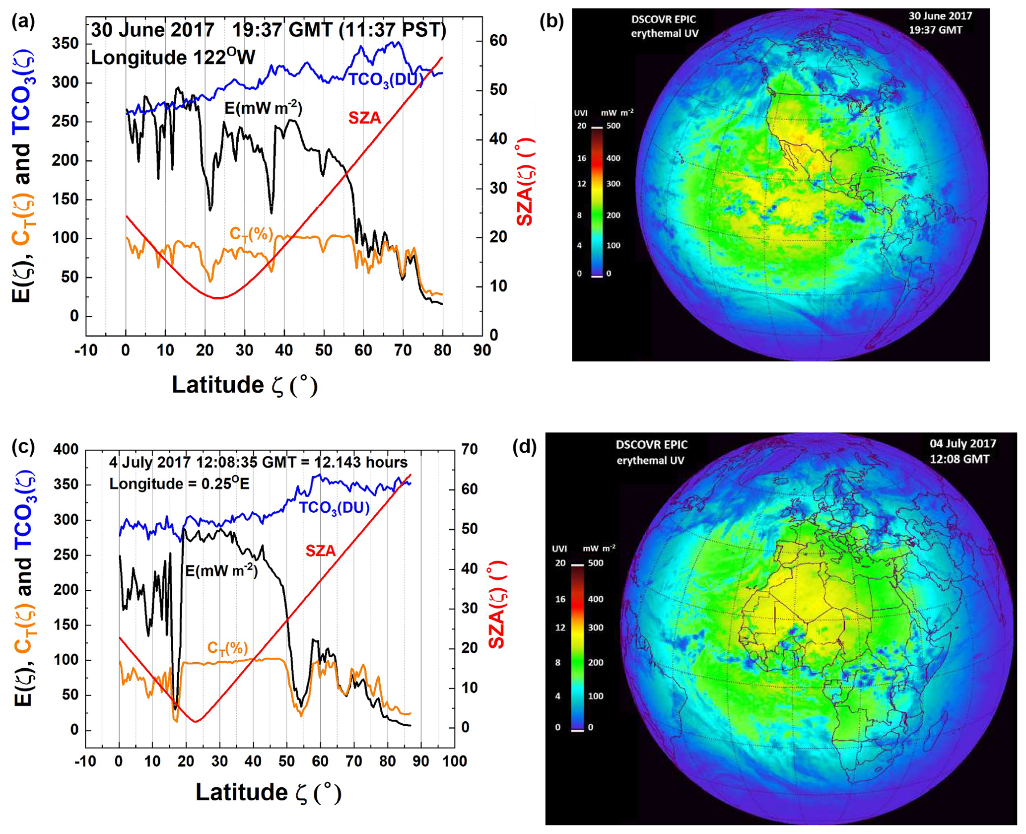
Figure 11 (a) Latitudinal distribution of E(ζ) and its contributing factors TCO₃, C_T, and SZA for a line of longitude passing through San Francisco, CA. (b) Global distribution of E(ζ,φ) from DSCOVR EPIC data on 30 June 2017 19:17 GMT when there were few clouds. Figure map created with IDL^®. (c) Latitudinal distribution of $E(\mathit{\zeta },\mathit{\phi },z,t)$ and its contributing factors TCO₃, C_T, and SZA for a line of longitude passing near Greenwich, England. (d) Global distribution of $E(\mathit{\zeta },\mathit{\phi },t_{\mathrm{O}}$) from DSCOVR EPIC data on 4 July 2017 12:08 GMT. Figure map created with IDL^®.

Figure 11a shows the latitudinal distribution, $\mathit{\zeta }=\mathrm{0}{}^{\circ }$ to 80^∘ N, of erythemal irradiance estimated from the synoptic EPIC measurements on a line of longitude passing through San Francisco, CA, at 19:37 GMT or 11:37 PST. The main driver of the decrease in E(ζ) from the Equator toward the poles is the increased optical path from increasing SZA(ζ) and increasing TCO₃(ζ) absorption. The smaller structure near 10, 21, and 37^∘ N is caused by small amounts of cloud cover reducing the transmission C_T(ζ). This day, 30 June 2017, near the 22 June solstice was selected based on the data from DSCOVR-EPIC showing that there were few clouds present in the scene (Fig. 11b) with C_T near 1. All the E(ζ) estimates in Fig. 11a are at or near sea level and yield a maximum UVI = 12 near 13^∘ N latitude. Similarly, Fig. 11c shows the latitudinal distribution of E(ζ) for the line of longitude passing near Greenwich, England, at 0.25^∘ E. E(ζ) is reduced because of cloud cover starting at 40^∘ N in addition to the increasing ozone absorption at higher latitudes. The accompanying images in Fig. 11b and d show the distribution of E(ζ) and the location of significant cloud cover.

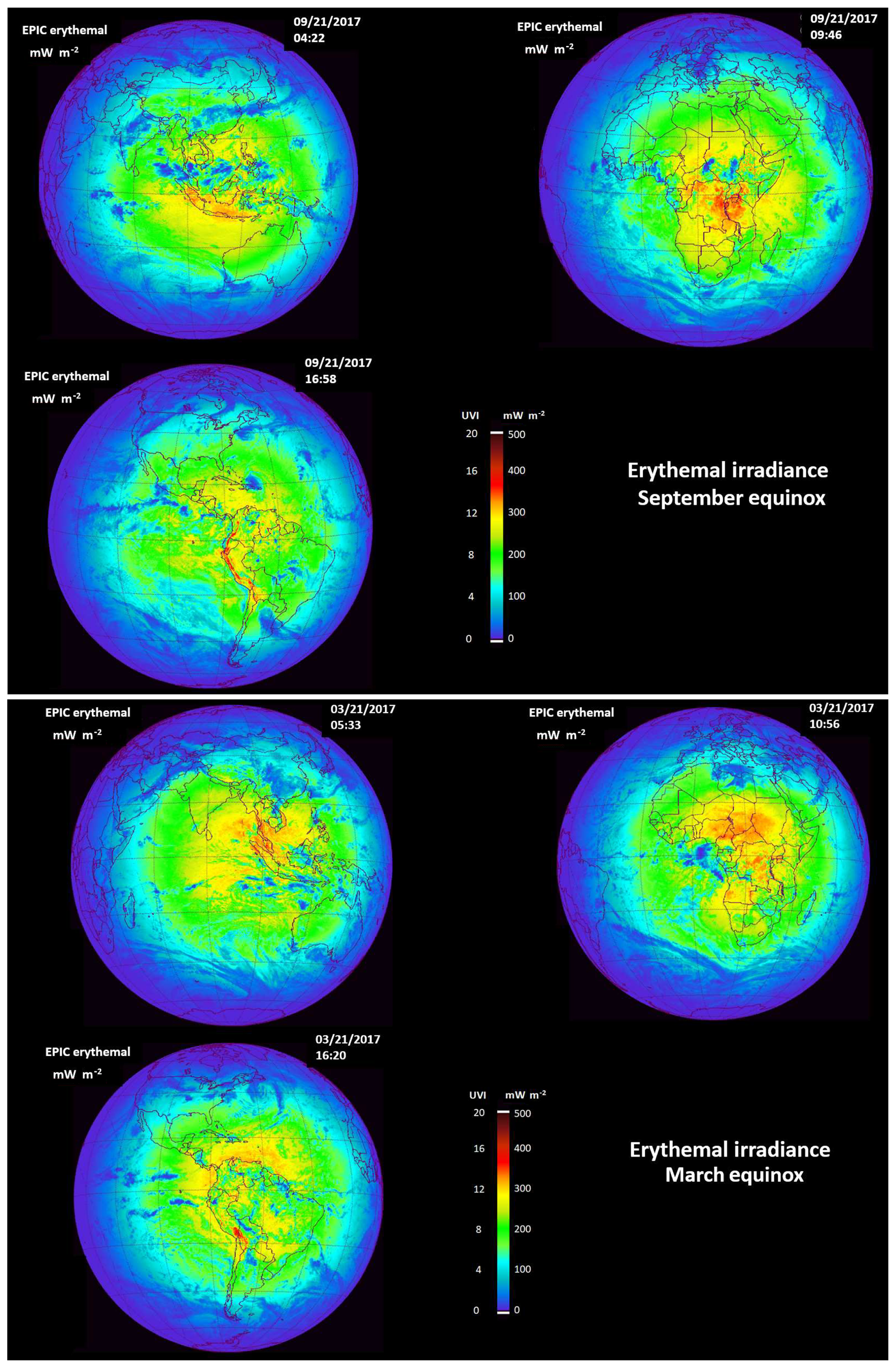
Figure 12 (a) $E(\mathit{\zeta },\mathit{\phi },t_{\mathrm{O}})$ and UVI($\mathit{\zeta },\mathit{\phi },t_{\mathrm{O}}$) from sunrise to sunset for the 21 September 2017 equinox. The three images are for different GMT. Figure map created with IDL^®. (b) $E(\mathit{\zeta },\mathit{\phi },t_{\mathrm{O}}$) and UVI($\mathit{\zeta },\mathit{\phi },t_{\mathrm{O}}$) from sunrise to sunset for the 21 March 2017 equinox. The three images are for different GMT (05:33, 10:56, and 16:20). Figure map created with IDL^®.

3.2 E(ζ, φ, t_O) for September and March equinox conditions

Near the September and March equinoxes (Fig. 12a and b) the Sun is overhead near the Equator, giving high UVI = 12 in many areas, with higher values (16 to 18) in the mountain regions (e.g., southern Indonesia, Peru's Andes Mountains, and some high-altitude regions in Malawi and Tanzania). While the Sun–Earth geometry is nearly the same for both equinoxes, there is considerable difference in seasonal cloud cover for the 2 equinox days. The area of sub-Saharan Africa near Nigeria has particularly high UVI values caused by nearly cloud-free conditions over a wide region, implying a considerable heath risk for midday UV exposure. Other high UVI values occur over smaller elevated areas. This is particularly evident in the nearly cloud-free high-altitude Peruvian Andes at about 28^∘ S even with SZA = 28^∘.

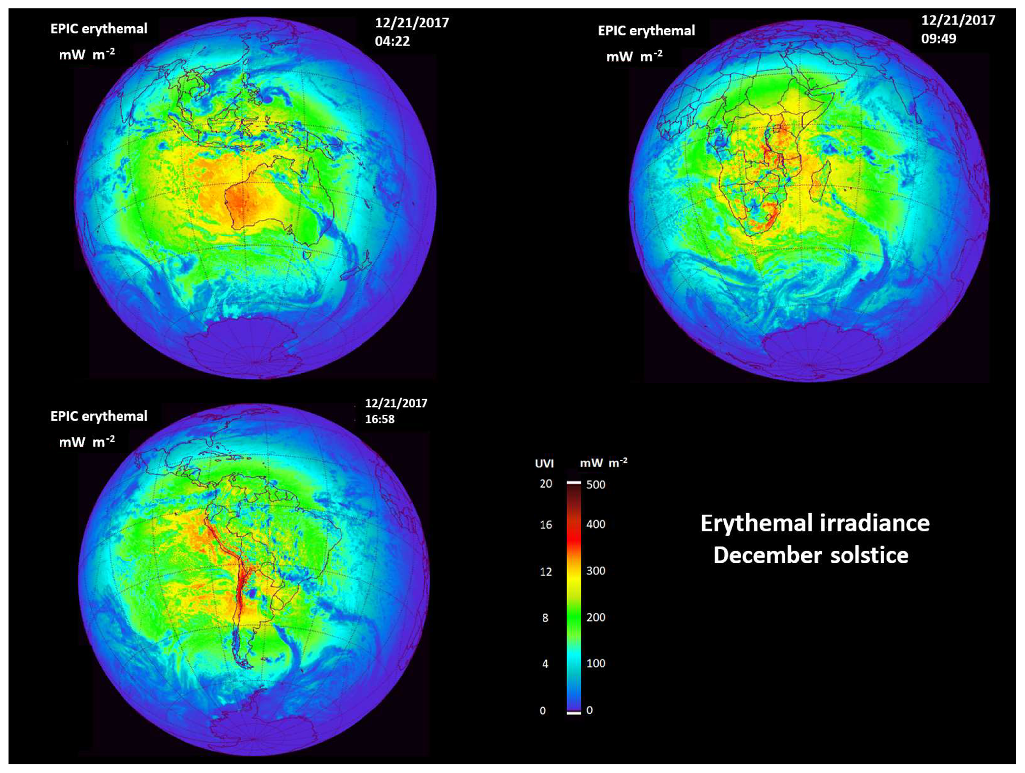
Figure 13 $E(\mathit{\zeta },\mathit{\phi },t_{\mathrm{O}})$ and UVI($\mathit{\zeta },\mathit{\phi },t_{\mathrm{O}}$) from sunrise to sunset for the 21 December 2017 solstice. The three images are for different GMT. Figure map created with IDL^®.

3.3 Southern Hemisphere summer solstice (December)

During the December solstice the Sun is overhead at 23.45^∘ S (Fig. 13). The reduced SZA causes high UVI levels throughout the Southern Hemisphere mid-latitude region, Fig. 13, between 20 and 40^∘ S, especially in elevated regions such as the Chilean Andes, Western Australia and elevated regions of southeastern Africa (South Africa, Tanzania, Kenya). For the case where Western Australia is near local solar noon, the UVI levels reach about 13 to 14 between 20 and 34^∘ S, a region that includes the city of Perth with more than a million people and several smaller cities and towns. These high UVI values represent a considerable health risk for skin cancer, since the UVI stays above 12 for nearly a month. This is also true for eastern Australia (Fig. 14) during December, which implies a high skin cancer risk for the entire Australian continent. The same comments apply to New Zealand, eastern South Africa and elevated areas further north (e.g., Tanzania, Africa). Even higher values occur in the Andes Mountains in Chile and Peru that include some small cities (see Fig. 6 for San Pedro de Atacama, Peru time series).

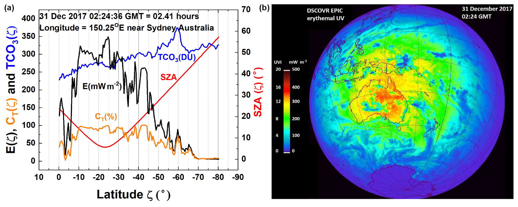
Figure 14 (a) Latitudinal distribution of $E(\mathit{\zeta },\mathit{\phi },z,t)$ and its contributing factors, TCO₃, C_T, and SZA, for a line of longitude passing near Sydney, Australia. (b) Global distribution of E(ζ,φ) from DSCOVR EPIC data on 31 December 2017 02:24:36 GMT. Figure map created with IDL^®.

Figure 14a shows the latitudinal distribution, 0 to 80^∘ S, of erythemal irradiance on a line of longitude passing near Sydney, Australia (population 5.3 million), at 02:24:36 GMT or 13:24 NSW (New South Wales). The main driver of the decrease in E(ζ) from the Equator toward the poles is the increased optical path from increasing SZA(ζ) and the increasing TCO₃(ζ). The smaller structures near 40, 50, and 60^∘ S are caused by small amounts of cloud cover reducing the transmission C_T(ζ). The 31 December day near the solstice was selected based on data from DSCOVR-EPIC showing that there were few clouds present over Australia (Fig. 6b). All the E(ζ) estimates in Fig. 14a are near sea level, with a maximum UVI = 14 near 25^∘ S latitude. Figure 14b shows the distribution of high E(ζ, φ) over Australia and Indonesia, with the highest values in Australia for 31 December 2017.

The erythemal irradiance differences between the northernmost city (Darwin, population 132 000) and the southernmost city (Melbourne, population 4.9 million) are quite large in terms of UV exposure because of differences in SZA, ozone amount, and cloud cover leading to a larger number of days per year with high UVI, a few weeks for Melbourne and 3 months for Darwin. This is reflected in the non-melanoma skin cancer statistics published by the Australian Institute of Health and Welfare (2016) for the different regions, with the Northern Territories (containing Darwin) having double the rate per 100 000 people compared to Victoria containing Melbourne (Pollack et al., 2014).

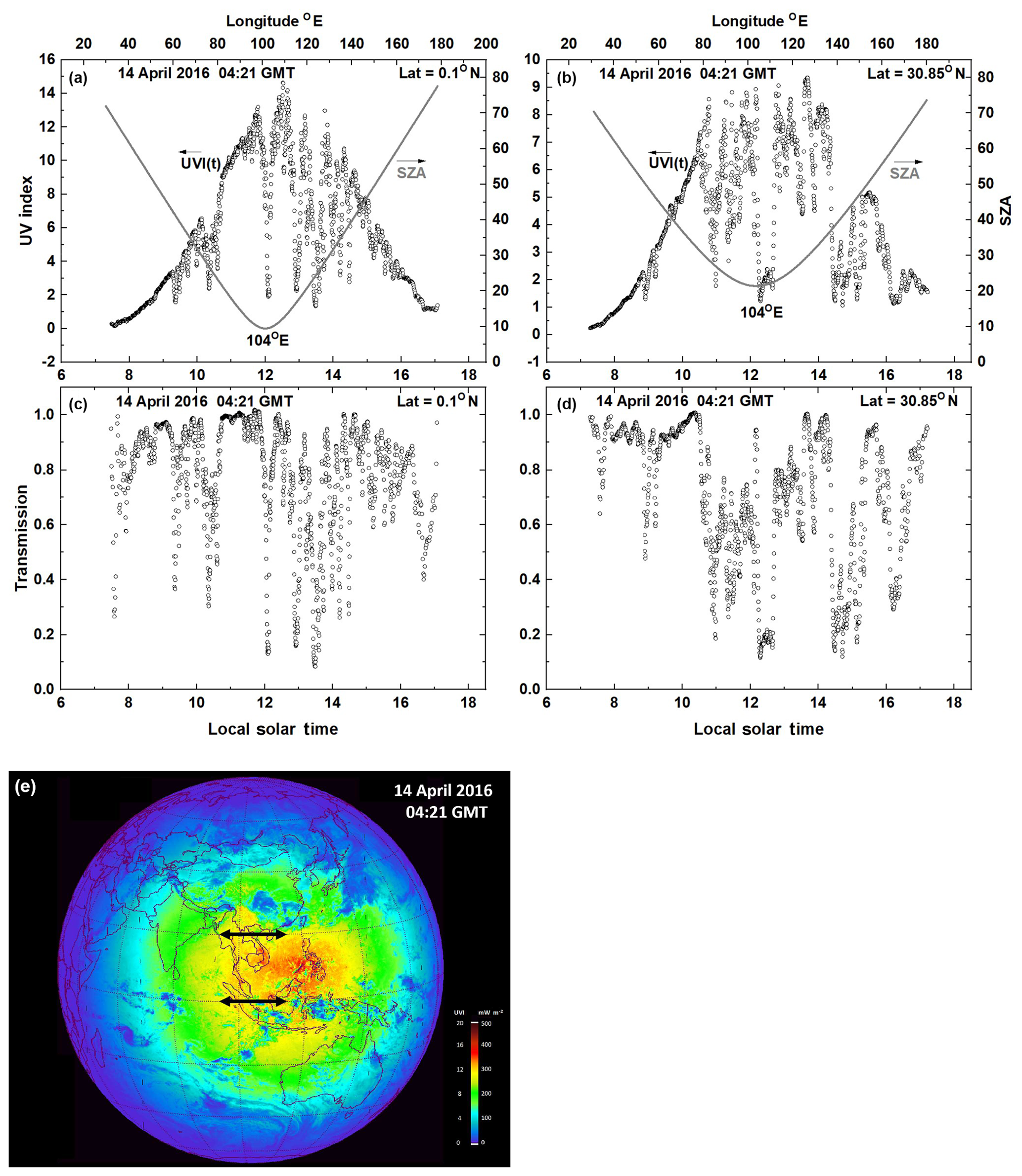
Figure 15 Longitudinal slices of UVI($\mathit{\zeta },\mathit{\phi },t_{\mathrm{O}}$) at 0.1 and 30.85^∘ N latitude (short dark horizontal arrows in e). The EPIC $E(\mathit{\zeta },\mathit{\phi },t_{\mathrm{O}})$ (mW m⁻²) images are for 14 April 2016 t_O=04:21 GMT centered at about 10^∘ N and 104^∘ E. (a, c) show longitudinal slices of $E(\mathit{\zeta },\mathit{\phi },t_{\mathrm{O}})$ and $C_{\mathrm{T}}(\mathit{\zeta },\mathit{\phi },t_{\mathrm{O}})$ for $\mathit{\zeta }=\mathrm{0.1}{}^{\circ }$ N and (b, d) for 30.85^∘ N. The solid lines in (a, b) represent the SZA. Figure map created with IDL^®.

3.4 Erythemal synoptic variation (sunrise to sunset)

The longitudinal dependence of E(ζ, φ, t_O) is illustrated in Fig. 15, where sunrise to sunset slices have been taken for an equatorial latitude, ${\mathit{\zeta }}_{\mathrm{o}}=\mathrm{0.1}{}^{\circ }$ N, and mid-latitude, ${\mathit{\zeta }}_{\mathrm{o}}=\mathrm{30.85}{}^{\circ }$ N. The estimated E(ζ_o, φ, t_O) includes the effect of clouds and haze (panels c and d) included in the atmospheric transmission function C_T(ζ_o, φ, t_O) and the effects of local terrain height. The maximum E(ζ_o, φ, t_O) is to the east of the sub-satellite point because the satellite orbit about the Lagrange-1 point L₁ is displaced to the west of the Earth–Sun line on 14 April 2016. The northward displacement is caused by the Earth's declination angle of about 9.6^∘. This corresponds to the minimum SZA shown in Fig. 15a of 9.5^∘. Panels a–d show the effects of cloud transmission for all values of LER that are not easily seen in the global erythemal color maps (bottom color panels of Fig. 15). The distribution of clouds is easily seen in the color image and LER image for 14 April at 04:21 GMT (Fig. 16a and b).

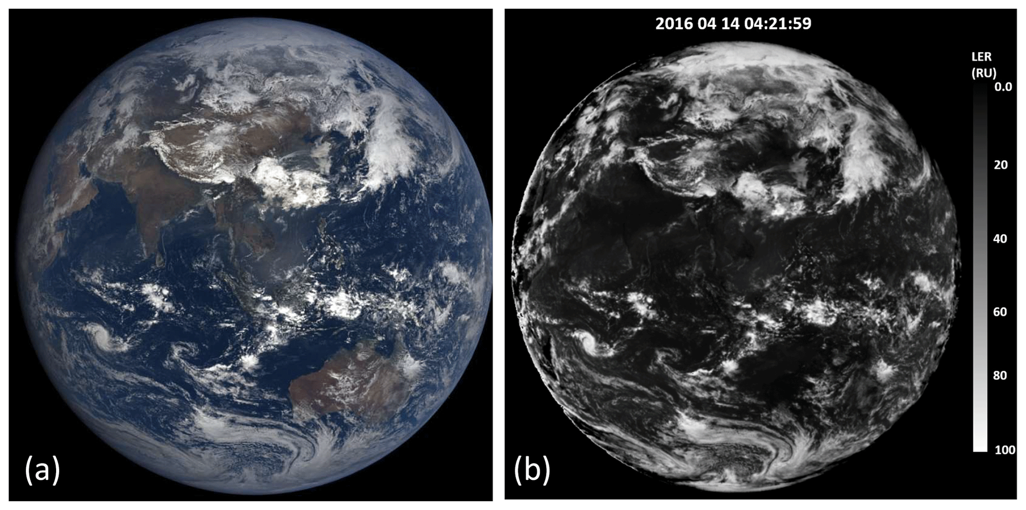
Figure 16 (a) EPIC color image for 14 April 2016 at 04:12:16 GMT showing the distribution of cloud cover and land corresponding to Fig. 15. https://epic.gsfc.nasa.gov/ (last access: 16 June 2020). (b) EPIC scene reflectivity LER for 14 April 2016 at 04:12:16 GMT.

The main cause of the decrease in E(ζ, φ, t_O) with latitude (Fig. 15a, b, e) between 0.1 and 30.85^∘ N is the increased SZA followed by the latitudinal increase in TCO₃. The difference is modulated (panels a and b) by the presence of clouds and haze (Figs. 15c, d and 16a, b) and haze in C_T(ζ, φ, t_O). There are nearly clear-sky patches for the equatorial slice (Fig. 15c) leading to very high UVI = 14 compared to the mid-latitude maximum of UVI = 9 because of the effect of clouds near the time of minimum SZA. The distribution of clouds is shown in the true color picture (Fig. 16a) of the Earth obtained by EPIC on 14 April 2016 at 04:12:16 GMT centered on 104^∘ E. The bright white portions of cloud images are the optically thick clouds of high reflectivity and low transmission. Comparing the color image to the LER image (Fig. 16b) illustrates how dark (unreflective) the land and oceans are in the UV compared to the visible wavelengths, even though clouds are reflective in both wavelength ranges. This allows cloud reflectivity and transmission C_T to be determined without complicated corrections for surface reflectivity for scenes free of snow and ice once Rayleigh scattering is removed.

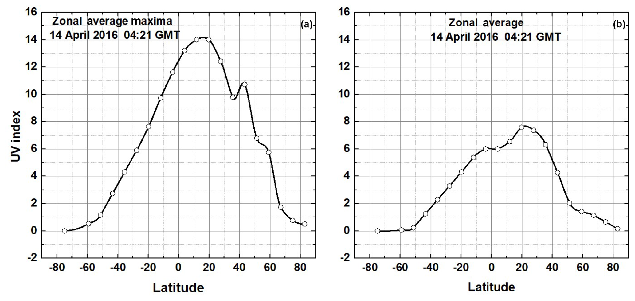
Figure 17 Zonal average of maximum UVI (UVIM a) and zonal average of mean UVI (UVIA b) on 14 April 2016 at 04:21 GMT from EPIC, including the effect of clouds and haze, as a function of latitude. Both the data points and an Akima spline fit are shown.

3.5 Zonal average E(ζ, φ, t_O)

Figure 17 shows a summary of the zonal average of maximum UVI (UVIM panel a) and zonal average of the mean UVI (UVIA panel b) values from EPIC on 14 April 2016 at 04:21 GMT from Fig. 14a for longitudinal band plots from $-\mathrm{75}{}^{\circ }$ < latitude < 75^∘. The solid lines are a smooth Akima spline fit (Akima, 1970) to the data points. Depending on the day of the year, the location of the maximum shifts between −23.45 and $+\mathrm{23.45}{}^{\circ }$ following the position of the overhead Sun. The zonal average UVIM (Fig. 17a) of about UVI = 14 is approximately the same for any day of the year. This includes longitudes containing high-altitude sites at moderately low latitudes where the local UVI maximum can reach 18 to 20. The US Environmental Protection Agency classifies exposure at UVI = 6 to 7 as high, which requires protection for extended exposure (e.g., 1 h). For low latitudes <30^∘, UVI > 6 occurs several hours around local solar noon. For equatorial latitudes at sea level, UVI > 6 occurs for about 6 h (Fig. 15). The zonal average values UVIA (Fig. 17b) are considerably smaller, since they are more affected by clouds than the mostly clear-sky maxima in Fig. 17a.

4 Summary

This study presents a global view based on satellite observations (OMI and EPIC) of the amount and changes for erythemal irradiance over major cities that are affected by ozone, clouds plus scattering aerosols, absorbing aerosols, and terrain height. While there is wide variation between specific sites, sites at high altitudes or low latitudes tend to have high values of UVI representing high levels of UV radiation that are dangerous to people with unprotected skin and eyes.

OMI-measured total column ozone TCO₃, Lambert equivalent reflectivity LER (converted to atmospheric transmission) data C_T(ζ, φ, z, t), and transmission reduction from aerosol absorption C_A(ζ, φ, z, t) from AURA-OMI data have been combined along with terrain height data to estimate noon erythemal irradiance $E(\mathit{\zeta },\mathit{\phi },z,t)$ time series globally distributed at 191 specified cities (see Fig. A3) using Eqs. (A1) to (A9). Fourteen-year site-specific changes in $E(\mathit{\zeta },\mathit{\phi },z,t)$ are derived from multivariate linear regression (MLR) trends (% yr⁻¹). For most sites, there has been no long-term MLR LS linear change (2005–2018) in UVI at the 2 standard deviation level 2-σ. Some of the sites do show 2-σ changes in UVI caused by changes in atmospheric transmission (clouds plus aerosols) and mostly an offset from zero caused by 14-year changes in OMI TCO₃. Fourteen-year trends as a function of latitude show the relationship between changes in ΔE and those from ΔC_T, ΔC_A, and ΔTCO₃. ΔE is correlated with significant decreases in ΔC_T and ΔC_A at southern latitudes 60 to 35^∘ S (Fig. 7c). There are significant decreases in ΔE around 5^∘ S and 22 and 35^∘ N, with a strong increase near 22.5^∘ N. For latitudes greater than 40^∘ N atmospheric transmission C_T has increased (cloud reflectivity decreased) for the period 2005 to 2018. Changes in ΔE caused by ΔC_T and ΔC_A are partially offset by ΔTCO₃ showing significant latitudinal increases at the 2-σ level between 25^∘ S and 20^∘ N and at high latitudes that only affect UV wavelengths (300–340 nm) sensitive to ΔTCO₃.

Some locations have extremely high values of UVI (12 < UV index < 18) caused either by the presence of low SZA and ozone values or high altitudes under almost clear-sky conditions. The maximum UVI is shown for each selected site (Table A4) with, as expected, low latitudes and elevated sites showing the highest UVI values (14 to 18) compared to typical mid-latitude sites at low altitude with a maximum UVI = 8 to 10. OMI-based results show agreement with the maximum seasonal values from several ground-based sites (Table 1) and with measurements of UVI made in Argentina (Cede et al., 2002, 2004). Two equatorial region high-altitude cities, San Pedro, Chile (2.45 km), and La Paz, Bolivia (3.78 km), with frequently clear-sky conditions have very high UVI_MAX=17 and 18 and UVI_AVG=11 in contrast to Quito, Ecuador (2.85 km), which has substantial cloud cover UVI_MAX=11 and UVI_AVG=7. Cities located at sea level in the equatorial zone also can have high vales of UVI_MAX=15 (e.g., Lima, Peru).

DSCOVR/EPIC global synoptic maps at a specified GMT of UVI from sunrise to sunset are shown for specific days corresponding to the solstices and equinoxes. These show the high UVI values occurring at local solar noon over wide areas and especially at high altitudes and the decrease with SZA caused by latitude and solar time. A zonal average of E for 14 April 2016 from EPIC data shows latitudes of very high UVI. For other days the latitudinal dependence and peak track the seasonal solar declination angle. EPIC observations show that there are wide areas between 20 and 30^∘ S latitude during the summer solstice in Australia (Fig. 12) showing near-noon values with UVI = 14 to 16, values that are dangerous for production of skin cancer and eye cataracts and that correlate with Australian National Institute of Health and Welfare cancer incidence health statistics (2016). Similar values of high UVI occur for the latitude range $\pm \mathrm{30}{}^{\circ }$ that includes parts of Africa and Asia.

Appendix A

Some of the contents of this Appendix are reproduced for convenience from Herman et al. (2018) and Herman (2010). Fitting error estimates from solutions of the radiative transfer equations are given in Herman (2010). The notation used in Herman (2010) and Herman et al. (2018) is retained with SZA (solar zenith angle), θ = SZA, Ω total column ozone amount in DU TCO₃, λ wavelength in nanometers, and C_T fractional cloud plus haze transmission. An improved numerical fit for the altitude dependence Z is provided for Eq. (A7) and for the coefficients in Eq. (A8).

Erythemal irradiance $E_{\mathrm{O}}(\mathit{\theta },\mathrm{\Omega },C_{\mathrm{T}},C_{\mathrm{A}})$ at the Earth's sea level (W m⁻²) is defined in terms of a wavelength-dependent weighted integral over a specified weighting function A(λ) times the incident diffuse plus direct solar irradiance I(λ, θ, Ω, C_T, C_A) W ∕ (nm m²) (Eq. A1). The erythemal weighting function Log₁₀(A_ERY(λ)) is given by the standard erythemal fitting function shown in Eq. (A2) (McKinley and Diffey, 1987). Tables of radiative transfer solutions for D_E=1 AU are generated for a range of SZA ($\mathrm{0}<\mathit{\theta }<\mathrm{90}{}^{\circ }$), for ozone amounts $\mathrm{100}<\mathrm{\Omega }<\mathrm{600}$ DU, and for terrain heights $\mathrm{0}<Z<\mathrm{5}$ km using accurate fitting functions to the solutions from the TUV DISORT radiative transfer model as described in Herman (2010) for erythemal and other action spectra (e.g., plant growth PLA, vitamin D production VIT, cataracts CAT). The irradiance weighted by the erythemal action spectrum is given by

$$\begin{array}{}\text{(A1)}& \begin{array}{rl}& E_{\mathrm{O}}(\mathit{\theta },\mathrm{\Omega },C_{\mathrm{T}},C_{\mathrm{A}})=\underset{\mathrm{250}}{\overset{\mathrm{400}}{\int }}I(\mathit{\lambda },\mathit{\theta },\mathrm{\Omega },C_{\mathrm{T}},C_{\mathrm{A}})A\left(\mathit{\lambda }\right)\mathrm{d}\mathit{\lambda },\\ & \mathrm{250}<\mathit{\lambda }<\mathrm{298}\mathrm{nm}{\mathrm{Log}}_{\mathrm{10}}\left(A_{\mathrm{ERY}}\right)=\mathrm{0},\\ & \mathrm{298}<\mathit{\lambda }<\mathrm{328}\mathrm{nm}{\mathrm{Log}}_{\mathrm{10}}\left(A_{\mathrm{ERY}}\right)=\mathrm{0.094}(\mathrm{298}-\mathit{\lambda }),\\ & \mathrm{328}<\mathit{\lambda }<\mathrm{400}\mathrm{nm}{\mathrm{Log}}_{\mathrm{10}}\left(A_{\mathrm{ERY}}\right)=\mathrm{0.015}(\mathrm{139}-\mathit{\lambda }).\end{array}\end{array}$$

Figure A1 Values of the coefficients R_ERY(θ) and U_ERY(θ).

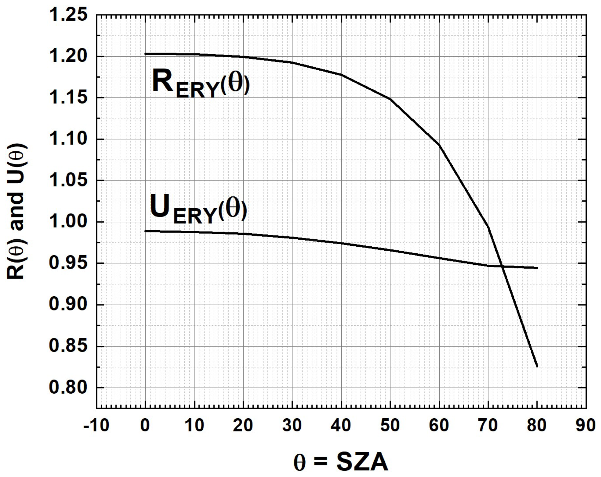
Table A1 Coefficients R(θ) and coefficient U(θ) for $\mathrm{0}<\mathit{\theta }<\mathrm{80}{}^{\circ }$, Eq. (A4), and $\mathrm{100}<\mathrm{\Omega }<\mathrm{600}$ DU for $E(\mathrm{\Omega },\mathit{\theta })=U\left(\mathit{\theta }\right)(\mathrm{\Omega }/\mathrm{200}{)}^{-R\left(\mathit{\theta }\right)}(\mathrm{1.0}E\mathrm{10}=\mathrm{1}\times {\mathrm{10}}^{\mathrm{10}}\left)U\right(\mathit{\theta })$ or $R\left(\mathit{\theta }\right)=(a+c{\mathit{\theta }}^{\mathrm{2}}+e{\mathit{\theta }}^{\mathrm{4}})/(\mathrm{1}+b{\mathit{\theta }}^{\mathrm{2}}+d{\mathit{\theta }}^{\mathrm{4}}+f{\mathit{\theta }}^{\mathrm{6}})r^{\mathrm{2}}>\mathrm{0.9999}$ (see Fig. A1).

Table A2 Solar zenith angle function G(θ) used in Eq. (A8). $G\left(\mathit{\theta }\right)=g+h\mathit{\theta }+i{\mathit{\theta }}^{\mathrm{2}}+j{\mathit{\theta }}^{\mathrm{3}}+k{\mathit{\theta }}^{\mathrm{4}}$.

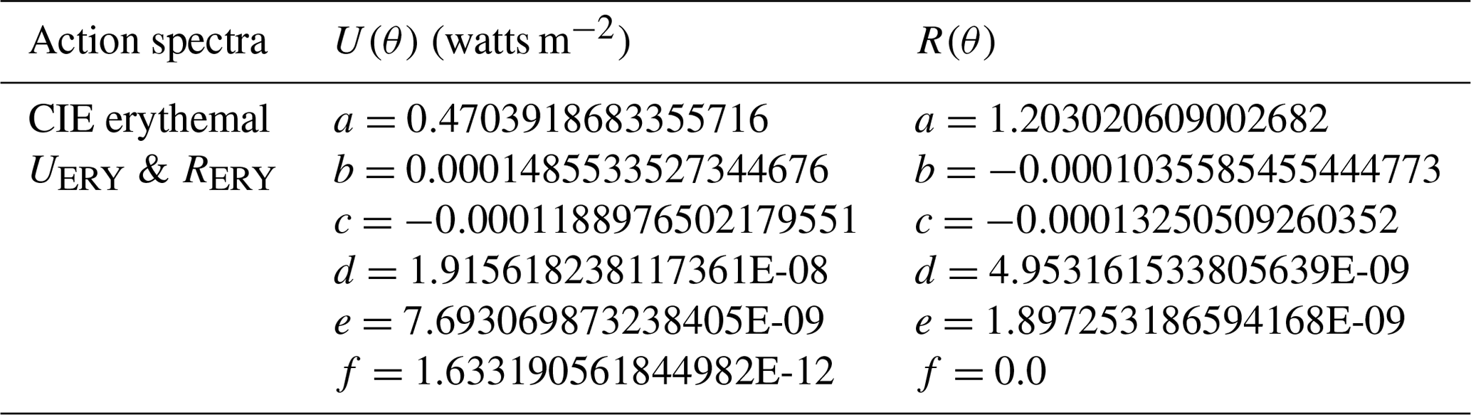
Equation (A1) can be closely approximated by the power law form (Eq. A3), where U(θ) and R(θ) are fitting coefficients where R(θ) is an improved radiation amplification factor (Herman, 2010) that is independent of Ω. Ozone independence arises because of an extra coefficient U(θ) representing E_O as a fit to the radiative transfer solutions in the form of rational fractions (Herman, 2010). Rational fractions were chosen because they tend to behave better at the ends of the fitting range than polynomials with comparable fitting accuracy. The absorbing aerosol reduction factor C_A is given by Eq. (2).

$$\begin{array}{}\text{(A2)}& \begin{array}{rl}& E_{\mathrm{O}}(\mathit{\theta },\mathrm{\Omega },C_{\mathrm{T}},C_{\mathrm{A}})=U\left(\mathit{\theta }\right)(\mathrm{\Omega }/\mathrm{200}{)}^{-R\left(\mathit{\theta }\right)}{C}_{\mathrm{T}}{C}_{\mathrm{A}},\\ & U\left(\mathit{\theta }\right)\text{or}R\left(\mathit{\theta }\right)=(a+c{\mathit{\theta }}^{\mathrm{2}}+e{\mathit{\theta }}^{\mathrm{4}})/\\ & (\mathrm{1}+b{\mathit{\theta }}^{\mathrm{2}}+\mathrm{d}{\mathit{\theta }}^{\mathrm{4}}+f{\mathit{\theta }}^{\mathrm{6}})r^{\mathrm{2}}>\mathrm{0.9999},\\ & C_{\mathrm{T}}=(\mathrm{1}-\text{LER})/(\mathrm{1}-R_{\mathrm{G}})\text{where}{R}_{\mathrm{G}},\\ & \text{is the reflectivity of the surface}\\ & E(\mathit{\theta },\mathrm{\Omega },z)=E_{\mathrm{O}}(\mathit{\theta },\mathrm{\Omega })H(\mathit{\theta },\mathrm{\Omega },z)/D_{\mathrm{E}}^{\mathrm{2}}.\end{array}\end{array}$$

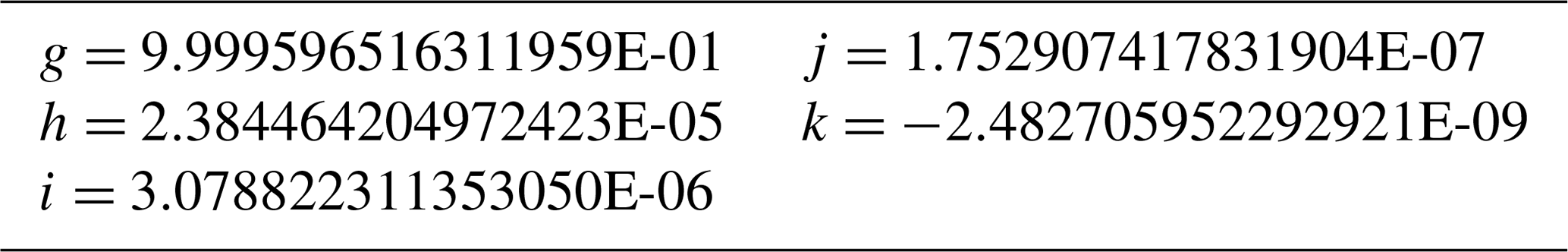
$H(\mathit{\theta },\mathrm{\Omega },Z)$ scales the erythemal irradiance at the surface to an altitude z and was calculated by fitting a function to the ratio $R_{\mathrm{E}}=E(\mathit{\theta },\mathrm{\Omega },z)/E_{\mathrm{O}}(\mathit{\theta },\mathrm{\Omega },\mathrm{0})$, where E and E_O were calculated with the TUV radiative transfer program. Most of the θ and Ω dependence is derived from E_O(θ,Ω). Linear extrapolation is used for Z>5 km, which gives almost the same result when TUV calculations are extended to 8 km.

$$\begin{array}{}\text{(A3)}& \begin{array}{rl}& H(\mathit{\theta },\mathrm{\Omega },Z)=\left[\right(-\mathrm{3.8443}E-\mathrm{3}{Z}_{\mathrm{km}}+\mathrm{3.1127}E-\mathrm{4})\\ & \mathrm{\Omega }/\mathrm{200}+\mathrm{0.054111}{Z}_{\mathrm{km}}+\mathrm{1}\left]G\right(\mathit{\theta }\left)G\right(\mathit{\theta })=g+h\mathit{\theta }\\ & +i{\mathit{\theta }}^{\mathrm{2}}+j{\mathit{\theta }}^{\mathrm{3}}+k{\mathit{\theta }}^{\mathrm{4}}\end{array}\end{array}$$

The coefficients $a,b,c,d,e,f,g,h,j$, and k are in Tables A1 and A2.

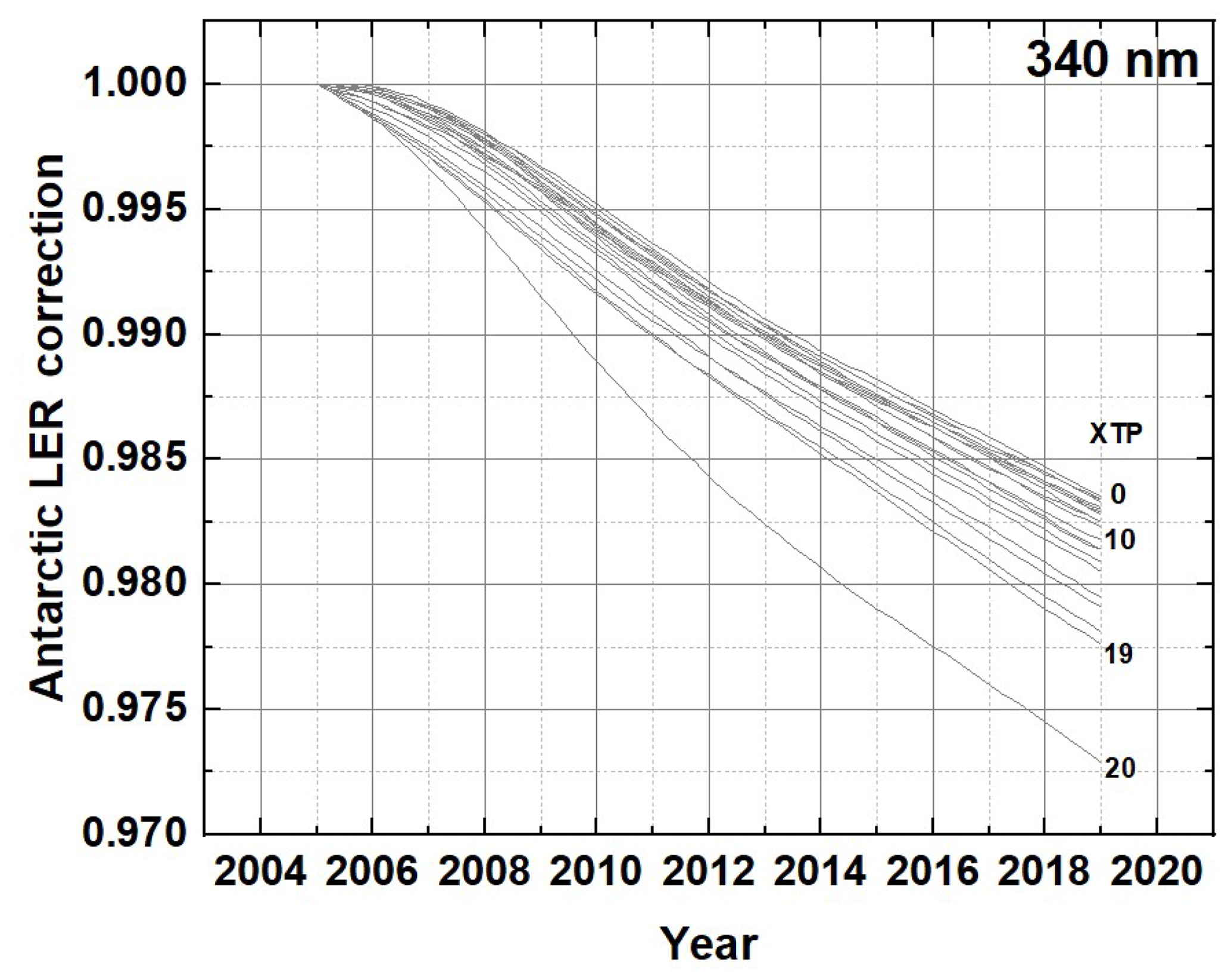
Figure A2 Correction factors for change in OMI sensitivity at 340 nm by measuring ice reflectivity over the Antarctic high plateau. For cross-track positions XTP 0 to 19, the change has been less than 2.5 %.

When Eq. (A6) is applied to the ozone and LER data, the global $E(\mathit{\theta },\mathrm{\Omega },z)$ at the Earth's surface can be obtained after correction for the Earth–Sun distance D_E, where D_E in AU can be approximated by Eq. (A9):

$$\begin{array}{}\text{(A4)}& D_{\mathrm{E}}=\mathrm{1}-\mathrm{0.01672}\cos \left(\mathrm{2}\mathit{\pi }\right(\text{day\_of\_year}-\mathrm{4})/\mathrm{365.25}).\end{array}$$

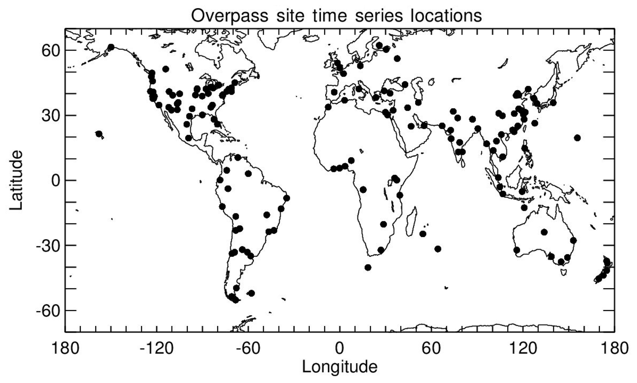
Figure A3 Map of locations in Table A4. Figure map created with IDL^®.

Since R_E(θ,Ω) has only weak θ and Ω dependence, an approximation can be obtained by forming the mean of R_E over θ and Ω. Then a linear approximation is

$$\begin{array}{}\text{(A5)}& H\left(z\right)=\mathrm{1}+\mathrm{0.047}{Z}_{\mathrm{km}}.\end{array}$$

Equation (A10) is similar to Eq. (A7) with G(θ)=1 and Ω=300 DU:

$$\begin{array}{}\text{(A6)}& H(\mathrm{300},Z)=\mathrm{1}+\mathrm{0.052}{Z}_{\mathrm{km}}.\end{array}$$

Note: double-precision coefficients are necessary for accuracy over the wide range of θ.

A similar approximate analysis can be obtained for height dependence of other action spectra given by Herman (2010) for Z_km=0 and the references therein.

Table A3 Height dependence of six action spectra.

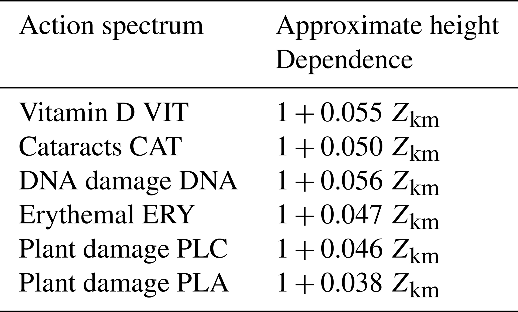
Height dependence increases for those action spectra with more emphasis on shorter UV wavelengths.

Over the 2005 to 2018 operating period of OMI there was a change in instrument sensitivity as measured by the reflectivity of the Antarctic high-plateau region (Fig. A2). The estimated OMI sensitivity change assumes that the summer reflectivity of the Antarctic high-plateau region has not changed. The small changes have little effect on ozone but directly affect LER.

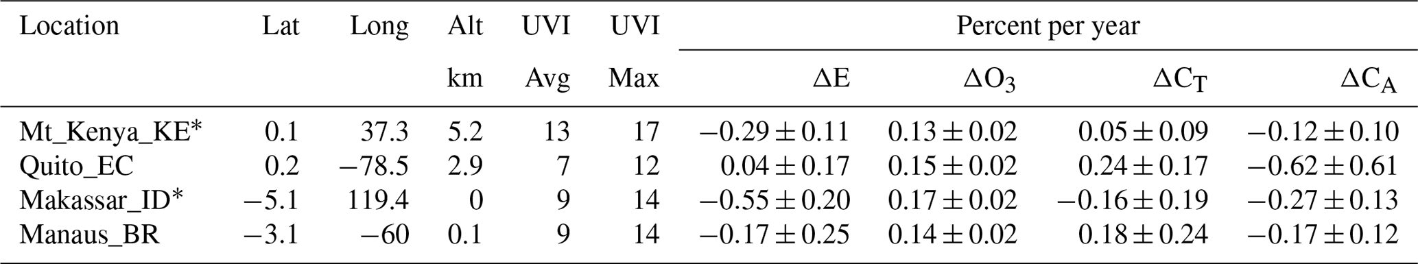
Table A4 summarizes the erythemal irradiance $E(\mathit{\theta },\mathrm{\Omega },z)$ and its rate of change ΔE for specific locations (latitude, longitude, and altitude) based on the algorithm from Eqs. (A1) to (A9). C_T includes the effect of both cloud and scattering aerosol transmission to the surface. Absorbing aerosols effects are included through the factor C_A. Sites that have trends statistically significant at the 2 standard deviation level (95 % probability) for $E(\mathit{\theta },\mathrm{\Omega },z,t)$ are indicated with an ^∗. For a number of sites, $E(\mathit{\theta },\mathrm{\Omega },z,t)$ can show significant change even when there is almost no change in Ω, where the change in $E(\mathit{\theta },\mathrm{\Omega },z)$ is caused by increases or decreases in C_A or C_T. The expected change in $E_{\mathrm{O}}(\mathit{\theta },\mathrm{\Omega },z,t)$ with ozone change ranges from about 0.82 to 1.2 (see R(θ) in Table A1 and Fig. A1) depending on the latitude (SZA as a function of latitude). Sites deviating significantly from this ratio have been affected by changes in C_T or C_A. A plot of these points plus ocean sites is shown in Fig. 7 and a map of the site locations in Fig. A3.

Table A4 191 land and city locations in various countries as indicated in alphabetical order. Shown are the latitude (Lat), longitude (Long), altitude (Alt), 14-year UVI average (Avg), 14-year average maximum (Max), average (AVG), and the trends Δ(E), Δ(O₃), Δ (C_T), and Δ(C_A) along with their accompanying 1 standard deviation uncertainties (1σ) (percent per year) for the erythemal irradiance with ozone, clouds and absorbing aerosols.

Δ is the slope B ± σ from Eq. (4) of the fit to each time series with 1 standard deviation σ. ^∗ indicates significant 2-σ change in E(t), TCO₃, C_T, and C_A.