the Creative Commons Attribution 4.0 License.
the Creative Commons Attribution 4.0 License.
 | 22 Jan 2020
Decoding long-term trends in the wet deposition of sulfate, nitrate, and ammonium after reducing the perturbation from climate anomalies
Xiaohong Yao
Long-term trends of wet deposition of inorganic ions are affected by multiple factors, among which emission changes and climate conditions are dominant ones. To assess the effectiveness of emission reductions on the wet deposition of pollutants of interest, contributions from these factors to the long-term trends of wet deposition must be isolated. For this purpose, a two-step approach for preprocessing wet deposition data is presented herein. This new approach aims to reduce the impact of climate anomalies on the trend analysis so that the impact of emission reductions on the wet deposition can be revealed. This approach is applied to a 2-decade wet deposition dataset of sulfate (), nitrate (), and ammonium () at rural Canadian sites. Analysis results show that the approach allows for statistically identifying inflection points on decreasing trends in the wet deposition fluxes of and in northern Ontario and Quebec. The inflection points match well with the three-phase mitigation of SO2 emissions and two-phase mitigation of NOx emissions in Ontario. Improved correlations between the wet deposition of ions and their precursors' emissions were obtained after reducing the impact from climate anomalies. Furthermore, decadal climate anomalies were identified as dominating the decreasing trends in the wet deposition fluxes of and at a western coastal site. Long-term variations in wet deposition showed no clear trends due to the compensating effects between NH3 emissions, climate anomalies, and chemistry associated with the emission changes of sulfur and nitrogen.
- Article
(4816 KB) - Full-text XML
-
Supplement
(345 KB) - BibTeX
- EndNote


To assess the long-term impacts of acidifying pollutants on the environment, the wet deposition of sulfate (), nitrate (), and ammonium (), among other inorganic ions, has been measured for several decades through monitoring networks such as the European Monitoring and Evaluation Programme (EMEP) (Fowler et al., 2005, 2007; Rogora et al., 2004, 2016), the National Atmospheric Deposition Program/National Trends Network in the US (Baumgardner et al., 2002; Lehmann et al., 2007; Sickles II and Shadwick, 2015), and the Canadian Air and Precipitation Monitoring Network (CAPMoN) (Vet et al., 2014; Zbieranowski and Aherne, 2011). The high-quality data collected from these networks have been widely used to quantify the atmospheric deposition of acidifying pollutants (Lajtha and Jones, 2013; Lynch et al., 2000; Pihl Karlsson et al., 2011; Strock et al., 2014; Vet et al., 2014). The data have also been utilized to identify trends in the atmospheric deposition of reactive nitrogen (Fagerli and Aas, 2008; Fowler et al., 2007; Lehmann et al., 2007; Zbieranowski and Aherne, 2011) and to examine the impacts of acid rain and the perturbation of the natural nitrogen cycle on sensitive ecosystems (Wright et al., 2018). The long-term data can also be used for assessing the effectiveness of environmental policies (Butler et al., 2005; Li et al., 2016; Lloret and Valiela, 2016).
The wet deposition of , , and is affected by not only their gaseous precursors' emissions (Butler et al., 2005; Fowler et al., 2007; Li et al., 2016) but also complex atmospheric processes such as long-range transport, chemical transformation, and dry and wet removal (Cheng and Zhang, 2017; Yao and Zhang, 2012; Zhang et al., 2012). These processes can be largely affected by climate anomalies. For example, climate anomalies can sometimes bring extreme precipitation amounts in a particular month and subsequently lead to extremely high wet deposition fluxes of ions through enhanced wet removal of air pollutants. Furthermore, climate anomalies can alter the relative contributions of local sources versus long-range transport to the total wet deposition amounts at reception sites, thereby complicating the relationships between wet deposition and the emission of air pollutants of interest (Lloret and Valiela, 2016; Monteith et al., 2016; Wetherbee and Mast, 2016). The emissions of SO2 and NOx have been decreasing substantially in Europe and North America (Butler et al., 2005; Li et al., 2016; Pihl Karlsson et al., 2011); coincidently, climate anomalies have also occurred more frequently in the recent decades (Burakowski et al., 2008; Lloret and Valiela, 2016; Wijngaard et al., 2003), thereby leading to more complicated linkages between wet deposition and emission trends on decadal scales.
Many trend analysis studies in the literature simply examined annual or seasonal values as the data inputs for two popular trend analysis tools, i.e., the Mann–Kendall (M–K) and linear regression (LR) methods (Marchetto et al., 2013; Waldner et al., 2014, and references therein). These studies focused on the detection of statistically significant trends; for example, Waldner et al. (2014) conducted a comprehensive analysis on the applicability of the techniques to different choices of length and temporal resolutions of a data series. Regarding the resolved trend results, these approaches are not well suited to separating the impact of air pollutants' mitigation from the perturbation by climate anomalies. Large uncertainties thus existed in the studies interpreting the major driving forces determining the extracted trends in the wet deposition of , , and . Regarding the fact that air pollutant emission mitigation targets often vary in different phases of the entire study period, inflection points may exist in the trends in the wet deposition of ions. The inflection points were rarely studied, despite their importance for assessing the effectiveness of environmental policies. An alternative would be to use high-time-resolution data in the ensemble empirical mode decomposition (EEMD) method (Wu and Huang, 2009); however, this method still suffers from the end effect in certain scenarios, whereby the extracted trends cannot be explained (Yao and Zhang, 2016).
A new approach is presented herein that aims to reduce the perturbations from climate anomalies of data inputs so that robust trends can be elucidated for evaluating the effectiveness of emission control policies. In this approach, raw data are preprocessed to generate a new variable, which is then applied to the M–K and LR methods. A piecewise linear regression (PLR) is also used to extract trends for cases in the presence of inflection points. The extracted trends in the wet deposition data on a decadal scale are then properly linked to major driving forces such as emission reductions and climate anomalies. This new approach is first applied to the wet deposition data of , , and in Canada, as an example to demonstrate its capability and advantages over the traditional approaches. The extracted trends in the wet deposition of ions are further studied through correlation analysis with known emission trends of their respective gaseous precursors (SO2, NOx, and NH3) in Canada and the US. Major driving forces for the trends of ion wet deposition and how the wet deposition ions responded to their precursors' emissions in Canada are then revealed.
2.1 Data sources
Wet deposition flux (Fwet) data were obtained from CAPMoN (https://www.canada.ca/en/environment-climate-change/services/air-pollution/monitoring-networks-data/canadian-air-precipitation.html, last access: 11 January 2020). Data from four sites have been collected for over 20 years and were chosen herein to illustrate the novel trend analysis method (Table S1 in the Supplement). Site 1 is an inland forest site at Chapais in Quebec. Site 2 is situated in a coastal forest area at Saturna in British Columbia. Sites 3 and 4 are two inland forest sites at the Chalk River and at Algoma, respectively, in northern Ontario. Details on data sampling, chemical analysis, and quality control can be found in previous studies (Cheng and Zhang, 2017; Vet and Ro, 2008; Vet et al., 2014).
The emissions data of gaseous precursors were downloaded from the Air Pollutant Emission Inventory (APEI, https://pollution-waste.canada.ca/air-emission-inventory/,last access: 11 January 2020) in Canada and from the US EPA National Emissions Inventory (NEI, https://www.epa.gov/air-emissions-inventories/air-emissions-sources, last access: 11 January 2020) in the US. These data were demarcated at a provincial level in Canada and at a state level in the US. Data for the years of 1990 to 2011, which correspond to the period of selected Fwet data, were used in this study.
2.2 Statistical methods
The M–K method is a popular nonparametric statistical procedure that can yield qualitative trend results, such as “an increasing/decreasing trend with a P value of <0.05,” “a probable increasing/decreasing trend with a P value of 0.05–0.1,” “a stable trend with a P value of >0.1 as well as a ratio of <0.1 between the standard deviation and the mean of the dataset,” and “no trend for P>0.1 with all other conditions” (Kampata et al., 2008; Marchetto et al., 2013). The LR method has also been widely used to extract trends (Marchetto et al., 2013; Waldner et al., 2014). Zbieranowski and Aherne (2011) used LR to extract trends by separating different phases because of the presence of inflection points in the entire study period, and the approach is the same as PLR (Vieth, 1989). In this study, the three methods were employed to compute the trends of ion wet deposition using software downloaded from https://www.gsi-net.com/en/software/free-software/gsi-mann-kendall-toolkit.html (last access: 11 January 2020) and Excel 2016, first using the annual Fwet directly as input data and then using a modified input dataset, as described in Sect. 2.3.
The annual Fwet is widely used for trend analysis, and the trend results are thereby used to compare with those derived from the approach proposed in this study. Note that R2 is conventionally used in LR and PLR. However, r instead of R2 is used in correlation analysis. Thus, R2 and r are used for the two types of analyses in this study. Moreover, several methods can be used to do PLR in classical statistics literature. The simplest one is to manually conduct piecewise regression where inflection points are visible to be recognized, and this approach is used in this study. More complex algorithms are also available in literature to conduct PLR for datasets with hundreds of points (Ryan and Porth, 2007, and references therein). The complex algorithms have seldom been used to identify trends in annual wet deposition of ions because of the short data record.
2.3 Filtering climate anomalies
The modified input dataset was produced in two steps. The first step was an effort to reduce the perturbation from the monthly climate anomalies to the input data. This was done by creating a new variable that was defined as the slopes of the regression equations of a series of study years against a climatology (base) year using monthly Fwet data. Note that the monthly Fwet data were aggregated from daily raw data before the regression analysis. To ensure the presence of enough data points in each regression equation, the data corresponding to 2-year periods (or 24 monthly Fwet values) were grouped together, as detailed below. At a selected site and for a given chemical component, monthly Fwet data were generated for the first 2 years and were grouped together and rearranged from the smallest to the largest values to form an array of data with 24 data points, i.e., A(i) with i=1 to 24. Repeating the above procedure for the subsequent years using a 2-year interval to eventually obtain a series of data arrays, A(i) now becomes A(i,j) with i=1 to 24 and j=1 to N, where N is the total number of data arrays. The climatology data array (CA(i)) was then defined as the average of all of the arrays as follows:
LR with zero interception was applied for each individual data array against the climatology data array. In cases where the maximum monthly deposition flux deviated greatly from the general regression curve, the slopes (m values) were calculated after excluding the maximum monthly deposition flux, which is an approach that reduced the perturbation to the m values from the monthly-scale climate anomalies. The second step was to screen out the outliers in m values, which reduced the perturbation to the m values from the annual-scale climate anomalies.
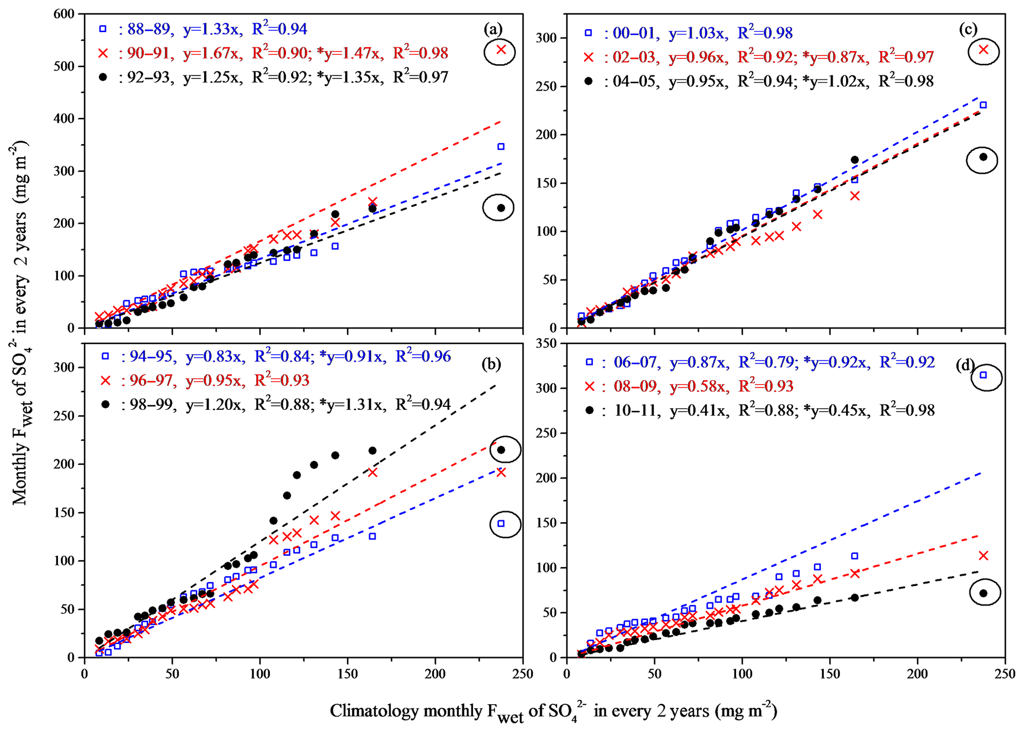
Figure 1Fitting monthly Fwet of against the climatology values from every 2 years using LR with zero interception at Site 1 according to the new approach described in Sect. 2. Fitted lines represent the LR function with zero interception using 24 elements. x, y, and R2 in the legend represent climatology monthly Fwet, monthly Fwet in every 2 years, and the coefficient of determination in LR analysis, respectively. The asterisk reflects the maximum value (cycled markers) excluded for LR analysis and all P values <0.01.
2.4 Example case for data filtering
An analysis of Site 1 is used to illustrate the new approach and demonstrate its advantages against the existing common approaches used in the literature. Twelve 2-year periods of data (1988–1989, 1990–1991, etc.) are available from this site. The regression of each dataset against the climatology dataset was first performed using all of the monthly values to obtain an m value (the slope) (Fig. 1a–d). For eight out of the 12 datasets, the m values were recalculated after excluding the maximum monthly value of Fwet, which appeared to be an apparent outlier of the linear regression. Three out of the 12 datasets showed the maximum Fwet being positively deviated from the general trend, five negatively deviated from the general trend, and four consistent with the general trend. The R2 values were then significantly increased for the eight sets, e.g., from the original values of 0.79–0.94 to the improved values of 0.92–0.98. To demonstrate that the excluded maximum value was an outlier, the case of the 1990–1991 dataset was taken as an example. The new regression equation (y=1.47x, R2=0.98, Fig. 1a) predicted a maximum value in the range of 330–368 mg m−2 month−1 using 3 times the standard deviation (±3 SD, 0.08) at a 99 % confidence level. The actual observed maximum value of 532 mg m−2 month−1 was much larger than the upper range of the predicted value and was thus believed to be caused by monthly-scale climate anomalies, i.e., the occurrence of an extreme amount of precipitation. The maximum monthly deposition flux in 1990–1991 occurred in September 1990 when the monthly precipitation depth reached 294 mm, which was much higher than that in the same month of other years, e.g., 169, 68, 95, and 127 mm in 1988, 1989, 1991, and 1992, respectively. The maximum daily precipitation depth in September was also higher in 1990 (91 mm) than in other years (43.6, 12.2, 13.6, and 26.8 mm in 1988, 1989, 1991, and 1992, respectively). However, the monthly geometric average concentration of in precipitation (1.8 mg L−1) in September 1990 was close to the mean value (1.7±0.3 mg L−1) in September 1988–1992 and was even smaller than that (2.9 mg L−1) in August 1990. The maximum value was treated as an outlier and excluded for analysis.
Using the similar procedure, all outliers in this study were identified. The exclusion of the observed maximum value greatly reduced the perturbation of the short-term climate anomalies to the calculated m value in this 2-year period; i.e., the m value decreased from 1.67 to 1.47, which in turn increased the relative contribution of the air pollutants' emissions to the calculated m value. Note that monthly changes in emissions may not impact the Fwet as much as a large monthly change in precipitation depth or concentration in precipitation does. For example, the monthly average concentrations of SO2 were almost the same in May, September, and October of 1990 (∼0.7 µg m−3) while the monthly Fwet of varied significantly, e.g., 113, 179, and 532 mg m−2 month−1 , respectively, in the same months. The monthly average concentration of SO2 in February (4.8 µg m−3) was the largest among the 12 months of 1990, but the corresponding monthly Fwet of was the smallest (34 mg m−2 month−1).
Even through comprehensive analysis, any single climate factor alone, including monthly precipitation depth, was apparently unable to explain the negative deviation of the maximum monthly value of Fwet from the general trend. The causes of such a negative deviation are yet to be identified. In summary, the new approach proposed above by applying the criteria of being outside the boundaries of ±3 times the standard deviation of the general trend meets the objective of identifying outlier data points.
The revised m values were further scrutinized by eliminating the outliers caused by the annual-scale climate anomalies. For example, the m value of 1.31 in 1998–1999 greatly deviated from other m values, narrowly oscillating approximately 0.96±0.07 (average ±1 SD) during the period of 1994–2005, even with the ±3 SD being considered (Fig. 1a–d). Using the value of 0.96 as the reference, climate anomalies likely increased the Fwet of by 37 % in 1998–1999. The m values were then calculated by shifting 1 year in time to 1997–1998 (1.07) and to 1999–2000 (1.24). The Fwet in 1998 was less affected by climate anomalies than that in 1999. Thus, the m value in 1997–1998 was within 0.96±0.21 (average ±3 SD) and used to replace the m value in 1998–1999 for the trend analysis. Similar to the first step discussed above, this approach meets the objective of identifying outlier m values by applying the criteria of being outside the range of ±3 SD plus the average m value during a decade or a longer period. The abnormally increased Fwet of in 1999 was mainly because of the increased precipitation depth (1312 mm), which was the largest during 1998–2011 (the annual average precipitation depth excluding 1999 was 1067±86 mm). However, the geometric average concentration of in precipitation in 1999 (1.0 mg L−1) was close to those in the other years, e.g., 0.9 mg L−1 in 1997 and 1998 and 1.0 mg L−1 in 2000.
2.5 Justification for the new approach
More justification of the new approach can be found in the Supplement, including Figs. S1–S6, wherein the statistical comparison between this and other approaches was presented. Theoretically, the extracted trend using the data preprocessed with the new approach is determined by the local emissions of air pollutants, the regional transport of air pollutants, and climate anomalies that are unable to be removed by the new approach. It is assumed that the extracted trend is less affected by microphysical/chemical processes, since 2-year data were used together to calculate the m value.
In theory, if the data from different sites in the same region are grouped together for trend analysis, the results may be better linked to the trends of the regional emissions of related air pollutants. In the following sections, trend analysis results from individual sites as well as those from grouped sites are discussed. Sites 1, 3, and 4 showed similar trends in the wet deposition of and , and these three sites were grouped together.
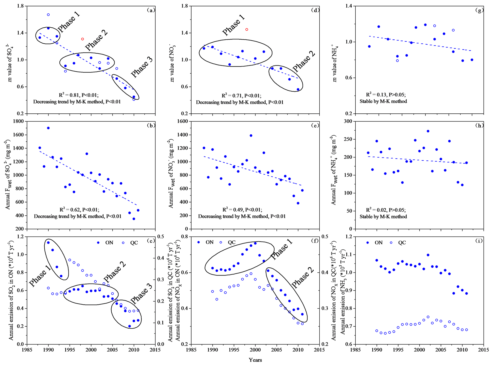
Figure 2The m values and annual Fwet of , and in 1988–2011 at Site 1, and the annual emissions of SO2 and NOx in 1990–2011 in Quebec and Ontario, Canada. Full and empty markers in blue in (a), (d) and (g) represent the calculation of m values without and with the outlier, respectively. Empty markers in red represent the outliers in m values and are excluded for trend analysis, as detailed in Sect. 2. R2 reflects the coefficient of determination of a variable against the calendar year from LR analysis, and the fitted lines represent the LR function. M–K results are shown in (a–b), (d–e) and (g–h). Phases 1, 2 and 3 in (a) and (c), Phases 1 and 2 in (d) and (f) were gained from PLR presented in Sect. 3.1.
3.1 Trends at Site 1 after reducing perturbations from climate anomalies
Trends in the m values shown in Fig. 2 represent the trends after removing the perturbations from climate anomalies at Site 1 in northern Quebec from 1988 to 2011. and showed decreasing trends from a LR analysis, with R2 values of 0.81 and 0.71, respectively, and P values <0.01 (Fig. 2a and d). The decreasing trends were also confirmed by the M–K method analysis. NHexhibited a stable trend from M–K analysis (Fig. 2g), as well as no significant trend with P value >0.05 from LR analysis. The annual Fwet values of these ions are also shown in Fig. 2b, e, and f, and annual emissions of SO2, NOx, and NH3 are shown in Fig. 2c, f, and i, respectively. These data were used to compare and facilitate analysis in terms of identifying inflection points and the advantage of using the m value over the annual Fwet, as presented below.
The m values of and also allowed for statistical identification of trends in different phases supported by annual variations in emissions of SO2 and NOx (Fig. 2c and f) to some extent. The inflection point for each phase is critical to (a) link the annual Fwet of ions and the emissions of the corresponding precursors and (b) assess the effectiveness of environmental policies. For example, the trends in the m values of can be clearly classified into three phases (Fig. 2a). Therefore, PLR should be applied separately for the different phases in the presence of the inflection points, rather than LR for the entire period, and the result is presented as
where x represents the calendar year from 1988 to 2010.
The m values oscillated approximately 1.38±0.08 during Phase 1 (1988 to 1993) and approximately 1.02±0.08 during Phase 2 (1994 to 2005), with a significant difference between the two phases under the t test (P value <0.01), thereby implying an abrupt decrease of approximately 30 % at the inflection point between the two phases. The m values linearly decreased by approximately 20 % every 2 years, starting from the end of Phase 2 to Phase 3 (2006–2011). Again, a significant difference existed between Phase 2 and Phase 3 under the t test (P value <0.01). The three phases generally aligned with the three-phase regulated SO2 emissions in Ontario. It should be stated that Phase 1 and Phase 3 each covered only 6 years (N=6). Cautions should be taken to explain the trend result in each phase in relation to precursors' emissions.
The PLR result of is expressed as
The trend in the m values of can be classified into two phases with the inflection point at 2003, which was confirmed by the t test result; i.e., the values oscillated approximately 1.09±0.09 during the period from 1988 to 2003 and then exhibited a significant decrease of approximately 50 % overall afterwards, with P value <0.01.
The m value of in 1998–1999 was approximately 30 % larger than the mean value in 1988–2003 and exceeded the mean value plus 3 SD in 1998–2003 and thus was not included in the trend analysis. The sharp increase in Fwet of occurred mainly in 1999, which was probably due to largely increased annual precipitation depth as mentioned in Sect. 2.4. The analysis was also supported by the geometric average concentration of in precipitation, which was 1.1 mg L−1 in 1999, 5 % lower than that in 1988 and only 5 %–10 % higher than those in 1990–1991, 1993, and 2002. Moreover, the monthly Fwet values of in March, April, July, and August 1999 were actually lower than the corresponding long-term averages in 1988–2003 (excluding 1999) (Fig. S6a). This outcome indicates that the large increase in annual Fwet of in 1999 was unlikely to have been determined by the emissions of its gaseous precursors. The same can be said for the large increase in Fwet of in 1999 (Figs. 2a, S6b).
To demonstrate the advantage of using the m values in trend analysis, m values were correlated to the reported emissions of concerned air pollutants. The trends in the m value of at Site 1 (Fig. 2a) were clearly different from those of the SO2 emissions in Quebec (Fig. 2c) but matched well to those in Ontario (Fig. 2c), which is also supported by their Pearson correlation coefficients, e.g., no significant correlation (r=0.46 and P value >0.05) for the former case and a good correlation (r=0.96 and P value <0.01) for the latter case. Zhang et al. (2008) reported that this remote area can receive the long-range transport of air pollutants from Ontario but that transport is less likely from the intensive emission sources in Quebec.
In addition, LR analysis of the annual Fwet of revealed a decreasing trend (second row in Fig. 2b). The M–K method analysis also confirmed the decreasing trend with annual Fwet as input. However, the three-phase trend in Fwet of and related inflection points, identified using the m values discussed above, were not identified by the t test when simply using annual Fwet data as input. The correlation between annual Fwet and emission was 0.89 for vs. SO2 in Ontario (P values <0.01), while the corresponding r value was as high as 0.96 between m value and emission. After reducing the perturbations from climatic factors to the annual Fwet, a stronger correlation was obtained between Fwet and emission. The increased r further solidified the dominant contribution of the long-range transport of air pollutants from Ontario rather than Quebec to the wet deposition of at Site 1.
The trends in NOx emissions during 1990–2003 had similar bell-shaped patterns in Quebec and Ontario, although with different magnitudes of emissions (Fig. 2f). A different trend pattern was seen for the m value of at Site 1 than for the abovementioned provincial emissions during the same period (Fig. 2d), and there was no significant correlation (r<0.41, with P value >0.05) between the m value of and the emissions of NOx in Quebec or Ontario. Different results were found for the period of 2002–2011 than those of 1990–2003 discussed above. In 2002–2011, the m value of decreased by ∼50 % and the NOx emissions decreased by ∼40 % in Quebec and Ontario; also, good correlations (r=0.94–0.95 with P values <0.01) were observed between m values and emissions. The contrasting correlation results between the two different periods discussed above implied the complex link between wet deposition of and emissions of NOx. One might assume that the perturbation from climate anomalies might not be fully removed by the new approach for the period of 1990–2003, which overwhelmed the effects of NOx emissions on the trends in m values of . Such a possibility is practically very low since the approach works well for the period of 2002–2011. The contrasting results between these two periods are yet to be explained. Fwet of and precipitation depth exhibited only a weakly significant correlation, with r=0.58 and P<0.05 in 1988–2003 (the values in 1999 were excluded). Annual precipitation varied by only ∼20 % during the 15 years, and this factor alone was unlikely to explain the ∼100 % interannual variation in Fwet of during that period.
LR analysis of the annual Fwet of revealed a decreasing trend (second row in Fig. 2e), confirmed by the M–K method analysis. However, the two-phase trend in Fwet of and related inflection point were not identified by the t test when simply using annual Fwet data as input. The correlations between annual Fwet and emission were 0.74–0.76 for vs. NOx in Quebec and Ontario (P values <0.01), while the corresponding r values increased to 0.84–0.85 between m value and emission. Both the identified inflection point and the stronger correlation between m value and emission demonstrated the advantage of using the m value over annual Fwet of in trend analysis.
The m value of at Site 1 had no significant correlation (r=0.21 and P value >0.05) with the emission of NH3 in Quebec but exhibited a weakly significant correlation (r=0.60 and P value <0.05) with the emission of NH3 in Ontario. Nearly all of the was associated with and in the atmosphere (Cheng and Zhang, 2017; Teng et al., 2017; Zhang et al., 2012), and the trends in the m value of could be affected by many other factors besides NH3 emissions and climate anomalies, e.g., gas–aerosol partitioning and different dry and wet removal efficiencies between NH3 and as well as pH value of wet deposition.
The stable trend in annual Fwet of and the decreasing trend in annual Fwet of gradually increased the relative contributions of reduced nitrogen in the total nitrogen wet deposition budget, e.g., from 40 % in 1998–1999 to 52 % in 2010–2011. A similar trend has also been recently reported in the US (Li et al., 2016). Such a trend was mostly due to the mitigation of NOx rather than climate anomalies.
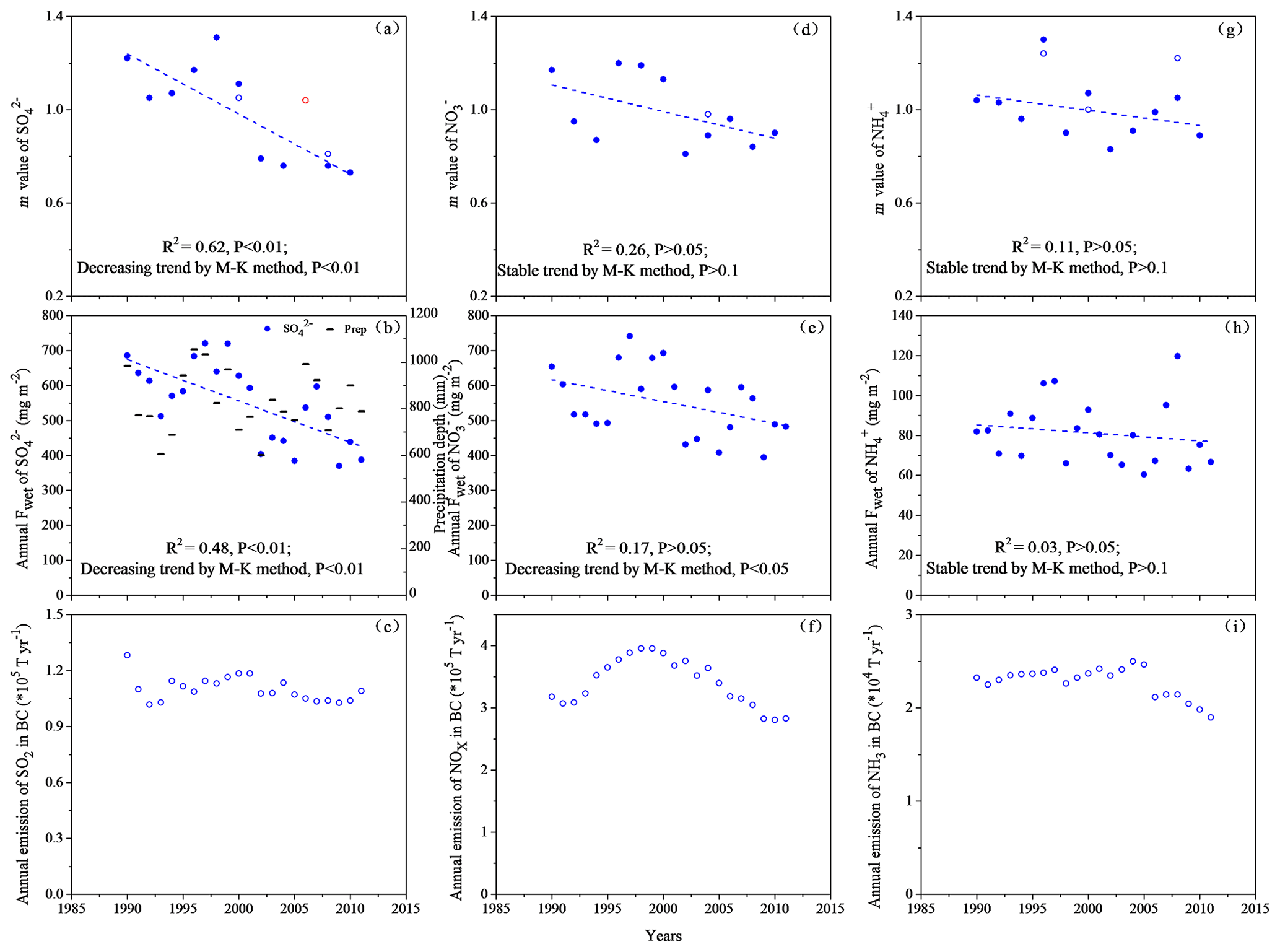
Figure 3Same as in Fig. 2 except for Site 2, and the annual precipitation and annual emissions in British Columbia, Canada. Horizontal dashes in (b) represent precipitation, and the fitted lines represent the LR function.
3.2 Decadal climate anomalies drove trends at Site 2
3.2.1 Trends in m value of SO
Figure 3 shows the trend analysis results at Site 2. An obvious shift in the m values and annual Fwet occurred during 2001–2002, as detected by the t test; i.e., the m values of oscillated approximately 1.15±0.11 in 1990–2001 and 0.76±0.02 in 2002–2011 (or 0.83±0.12 if the value in 2006–2007 was included), but with a significant difference between the two periods with a P value <0.01. The annual Fwet of oscillated approximately 632±63 mg m−2 in 1990–2001 and 452±74 mg m−2 in 2002–2011, and the values between the two periods showed significant differences. The shift led to the m values and annual Fwet of exhibiting a consistent decreasing trend by ∼40 % overall from 1990 to 2011 using the LR and the M–K methods.
The emissions of SO2 oscillated approximately 1.13±0.07 in 1990–2001 and 1.06±0.03 in 2002–2011 in British Columbia, which did not support the large decrease of approximately 40 % in wet deposition of in 2002–2011. Statistically, no correlation existed between annual Fwet of and the emissions of SO2 in British Columbia, with r=0.52 and a P value >0.05. Although the transboundary transport of air pollutants from the US cannot be excluded, the almost constant m values from 2002 to 2011 (excluding 2006–2007) at Site 2 were inconsistent with the approximately 70 % decrease in emissions of SO2 in the state of Washington in the US during that period (not shown). Precipitation cannot explain the jump in wet deposition either, because there was no corresponding jump in precipitation during 2001–2002 (Fig. 3b).

Figure 4The mean wind vector and speed (shading area) during 1990–2011 (a) and the anomalies of wind vector and wind speed (shading area) during 1990–2001 (b), 2002–2011 (c), and 2007 (d) at 925 hPa over western coastal Canada and the US (the anomalies in b, c, and d were conducted relative to the 20-year period of 1990–2009 and the wind vector and wind speed were from the North American Regional Reanalysis (NARR) with a spatial resolution of 32 km by 32 km).
Van Donkelaar et al. (2008) analyzed aircraft and satellite measurements from the Intercontinental Chemical Transport Experiment and proposed the long-range transport of sulfur from East Asia to the west coast of Canada. The wind vector and wind speed from the North American Regional Reanalysis (NARR), with a spatial resolution of 32 km by 32 km (Mesinger et al., 2006), were thereby analyzed to study the decadal changes in wind fields and associated potential impacts on the long-range transport of air pollutants over western coastal Canada and the US. The average wind fields including mean wind vector and speed (shading in Fig. 4a–d) in 1990–2011 at 925 hPa showed air masses over western coastal Canada and the US primarily originated from the Pacific Ocean (Fig. 4a). However, the anomalies of wind fields in 1990–2001 relative to 1990–2009 clearly showed a counterclockwise pattern in the corresponding coastal area, including Site 2, while a clockwise pattern existed in 2002–2011 relative to 1990–2009 (Fig. 4b, c). The anomalies shown in Fig. 4c indicated the northwesterly wind being enhanced in 2002–2011 over western coastal Canada and the US, possibly reducing air pollutants being transported from the continent to Site 2. In contrast, the anomalies in Fig. 4b indicated that the northwesterly wind was reduced in 1990–2001. Consequently, more air pollutants might have been transported from the continent to Site 2, resulting in a distinct demarcation in 2002. This hypothesis was also supported by a large rebound of the m value in 2006–2007, due to the increase in Fwet of in 2007. The climate anomalies of wind fields in 2007 relative to 1990–2009 showed a counterclockwise pattern in the north, while the clockwise pattern was pushed to the south (Fig. 4d). With the northwesterly wind being reduced, a greater contribution of air pollutants from the coast of Canada and US to Site 2 might have led to the large increase in Fwet of during a few month-long periods in 2007.
The present study is the first one identifying the decreasing trend in the annual Fwet of as being very likely caused by decadal climate anomalies, i.e., wind fields, rather than by the emission reductions of SO2. The decadal anomalies of wind fields may substantially alter the long-range transport of air pollutants to the reception site. Note that the causes for the decadal anomalies of wind fields in this region are beyond the scope of the present study, but some information can be found in the literature (Bond et al., 2003; Coopersmith et al., 2014; Deng et al., 2014).
3.2.2 Trends in m values of NO and NH
For the wet deposition of , the m values also showed a clear shift; i.e., the m values oscillated approximately 1.09±0.14 in 1990–2001 and 0.88±0.06 in 2002–2011, with a significant difference between the two periods under the t test with a P value <0.01. The annual Fwet of varied substantially, and the shift could not be identified statistically. However, the annual Fwet of exhibited a decreasing trend with M–K method analysis. Similar to the case of , no significant correlation (r=0.49, P value >0.05) existed between the annual Fwet of and the emissions of NOx in British Columbia.
In addition to decadal anomalies of wind fields, the interannual climate variability such as precipitation depth, annual anomalies of wind fields in 2007, etc., (Fig. 3b) also affected the trends in m values and annual Fwet of . The annual precipitation depth largely varied from 601 mm to 1054 mm in the 2 decades. The perturbations from interannual variability of precipitation depth cannot be completely removed by the new approach. For example, the calculated m values in 1992–1993 and 1994–1995 were evidently lower than the m values in 1990–2001. However, the annual geometric average concentrations of in 1992–1995 varied around 0.77±0.11 mg L−1 and were even larger than the values of 0.66±0.08 mg L−1 in 1990–2001 (excluding 1992–1995). The lower m values were mainly attributed to the lower precipitation depth in 1992–1994 (Fig. 3b) rather than lower emissions of NOx. Interannual climate variability including precipitation depth and annual anomalies of wind fields may complicate the relationship between the Fwet of and the emissions of NOx in British Columbia. For example, the m values in 1990–1991, 1996–1997, 1998–1999, and 2000–2001 were nearly constant at 1.17±0.03; however, the NOx emissions in British Columbia in 1998–1999 were 26 % greater than those in 1990–1991. Moreover, there was a sharp decrease in the NOx emissions (by ∼30 %) from 2002 to 2011 in British Columbia. However, the m values oscillated approximately 0.88±0.06 and showed no clear trend based on either the M–K method or LR analysis. The interannual climate variability apparently negated the impact of reduced emissions during these periods.
The m values and the annual Fwet of oscillated approximately 0.99±0.13 and 81±16 mg m−3, respectively, in the period of 1990–2011 and showed no trend (Fig. 3). Neither the m values nor annual Fwet of showed the two-period distribution pattern or had any significant correlation with the emissions of NH3 in British Columbia at a 95 % confidence level. Similarly to Site 1, the annual variation in Fwet of at Site 2 cannot be simply explained by known emission trends.
In summary, decadal anomalies of wind fields overwhelmingly determined the long-term trends in the wet deposition of and , with the perturbation from monthly and annual climate anomalies removed at Site 2. The interannual climate variability including precipitation depth, annual anomalies of wind fields, etc. further complicated the trends, resulting in undetectable influences of the emission trends on the deposition trends. Since the decrease in Fwet of appeared to be primarily caused by decadal climate anomalies of wind fields, the relative contributions of and in the total N wet deposition varied little, i.e., 33 % versus 67 % in 2010–2011 and 31 % versus 69 % in 1990–1991.
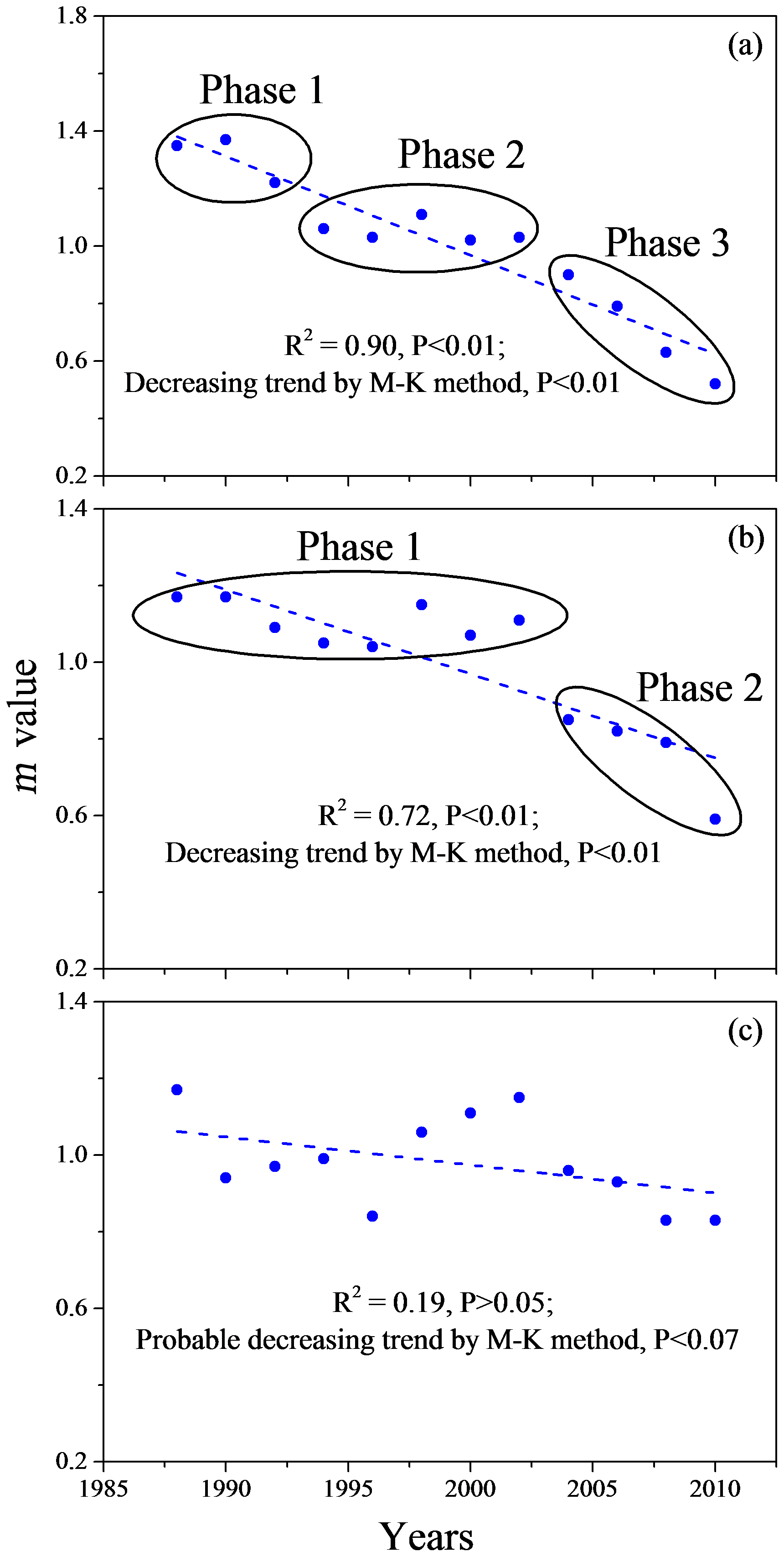
Figure 5Regional m values at Sites 1, 3, and 4: (a) , (b) , and (c) . R2 reflects the coefficient of determination of a variable against the calendar year from LR analysis, and the fitted lines represent the LR function. M–K results are shown in (a–c). Phases 1, 2, and 3 shown in (a) and Phases 1 and 2 shown in (b) were gained from PLR presented in Sect. 3.3.
3.3 Regional trends in wet deposition in northern Ontario and Quebec
Trends in the m values or annual Fwet of ions at Sites 3 and 4 in the northern regions of Ontario were generally similar to those found at Site 1 (Figs. S7 and S8). The three-phase trend in m values of and the two-phase trend in m values of were also obtained at Sites 3 and 4 after excluding a few m values that were caused by large perturbations from climate anomalies. For example, the annual precipitation depths of 1044 mm in 1987 and 905 mm in 1997 at Site 4 were evidently lower than the average value of 1299±124 mm (excluding 1987 and 1997) in 1985–1997 (Table S2). However, the geometric average concentration of of 1.5 mg L−1 in 1997 was the same as the mean value of 1.5±0.2 mg L−1 in 1995–1999 (excluding 1997). The value of 1.6 mg L−1 in 1987 was also the same as that in 1989. The lower annual precipitation depths in 1987 and 1997 than in the other years were very likely the dominant factor causing the abnormally lower m values in 1986–1987 and 1996–1997. Thus, Sites 1, 3, and 4 were combined together to study regional trends in the northern areas of Ontario and Quebec (Fig. 5a–c). Similar to those found at the individual sites, the temporal profile of regional m values of can be clearly classified into three phases (Fig. 5a) as follows: Phase 1 from 1988 to 1993 with m values oscillating approximately 1.31±0.08, Phase 2 from 1994 to 2003 with near-constant m values of 1.05±0.04, and Phase 3 for 2004 onward with a decreasing trend by overall ∼50 %. Significant differences of m values existed between any two of the three phases, based on the t test results (P value <0.01). The PLR result is expressed as below:
The three-phase pattern of m values matched well with the three-phase emission profile of SO2 in Ontario. Statistically, an ∼70 % decrease in m value and an ∼70 % decrease in emissions were found from 1990 to 2011, with a correlation of r=0.95 (P value <0.01).
The profile of the regional m values of also clearly exhibited two phases, according to the following t test results: Phase 1 from 1988 to 2003, with m values narrowly varying approximately 1.11±0.05, and Phase 2 from 2004 to 2011 with a decreasing trend by an overall ∼40 % against that in 2002–2003 (Fig. 5b). The PLR result is expressed as below:
From 2002 to 2011, the m value had a moderately good correlation with the NOx emission in Ontario (r=0.91, P<0.01), and the two variables decreased by 30 %–40 % in this period. From 1990 to 2003, the near-constant m value was, however, inconsistent with the bell-shaped profile of the NOx emissions mainly caused by annual variations in NOx emission from the sector of transportation and mobile equipment in Ontario and Quebec, which could be due to either the perturbation from climate anomalies or an unrealistic emissions inventory from (APEI) in Canada. Considering that the first possibility was minimal over a large regional scale, especially when the consistency was determined in a different time frame (2002–2011) in the same region, it is thus doubtful that the bell-shaped profile of the NOx emissions in 1990–2003 was realistic.
The regional m values of largely oscillated from 1988 to 2003 (Fig. 5c). The m values of , however, decreased by ∼30 % from 2002 to 2011, leading to a probable decreasing trend in the m value from 1988 to 2011. No correlation was found between the m values of and the emissions of NH3 in Ontario, which is consistent with the findings at the individual sites discussed above.
Since the decrease in Fwet values of at Sites 3 and 4 was very likely due to the mitigation of NOx in Ontario, the decrease also changed the relative contributions between and in the total N wet deposition budget. For example, and contributed 52 % and 48 %, respectively, to the total budget in 2010–2011 and 34 % and 66 %, respectively, in 1984–1985 at Site 3. The corresponding numbers at Site 4 were 58 % and 42 % in 2010–2011 and 47 % and 53 % in 1985–1986.
Climate anomalies during the 2-decade period resulted in annual Fwet of and/or deviating from the normal value by up to ∼40 % at the rural Canadian sites. The new approach of rearranging and screening Fwet data can largely reduce the impact of climate anomalies when used for generating the decadal trends of Fwet. With the climate perturbation being reduced, Fwet of exhibited a three-phase decreasing trend at every individual site, as well as on a regional scale in northern Ontario and Quebec. The three-phase pattern of the decreasing trend in Fwet of matches well with the emission trends of SO2 in Ontario, as supported by the good correlation between wet deposition and emission, with r≥0.95 and P<0.01. Fwet of exhibited a two-phase decreasing trend, but only during the second phase Fwet of , and the emissions of NOx in Ontario and Quebec matched well, with a good correlation of r≥0.91 and P<0.01. Compared to the results obtained without applying the new approach, it is concluded that, after reducing the perturbation from climate anomalies, (1) better correlation was obtained between Fwet of ions and the emission of the corresponding gaseous precursors in northern Ontario and Quebec, and (2) the inflection points in the decreasing trends of Fwet of and were visibly and statistically identified.
However, the new approach cannot completely remove the perturbations from climate anomalies, especially when this is the dominant factor and/or on long timescales, as was the case at a coastal site of Saturna in British Columbia. At this location, the decreasing trends in Fwet of and were caused by the decadal anomalies of wind fields, as well as being affected by interannual climate variability including precipitation depth and annual anomalies of wind fields, which overwhelmed the impact of the emission changes of the gaseous precursors in this province. This is the first study that has identified that decadal anomalies of wind fields can dominate trends in Fwet of and . The new findings will stimulate more studies on the impacts of decadal climate anomalies on atmospheric deposition of concerned air pollutants. The long-term variations in Fwet of generally showed no clear long-term trends. Moreover, no apparent cause–effect relationships were found between the wet deposition of and the emission of NH3. It can be reasonably inferred that additional key factors besides those discussed in this study also impact the trends of Fwet of . Thus, cautions should be taken to use wet deposition fluxes of to extrapolate emissions of NH3.
Data used in this study are available from the corresponding authors.
The supplement related to this article is available online at: https://doi.org/10.5194/acp-20-721-2020-supplement.
XY and LZ designed the study, analyzed the data and prepared the paper.
The authors declare that they have no conflict of interest.
We greatly appreciate the reviewers for their constructive comments which have helped us improve the paper quality.
This research has been supported by the National Key Research and Development Program in China (grant no. 2016YFC0200500) and the Climate Change and Air Pollutants program of Environment and Climate Change Canada (grant no. N/A).
This paper was edited by Aijun Ding and reviewed by G. M. Beachley and one anonymous referee.
Baumgardner, R. E., Lavery, T. F., Rogers, C. M., and Isil, S. S.: Estimates of the Atmospheric Deposition of Sulfur and Nitrogen Species: Clean Air Status and Trends Network, 1990–2000, Environ. Sci. Technol., 36, 2614–2629, https://doi.org/10.1021/es011146g, 2002.
Bond, N. A., Overland, J. E., Spillane, M., and Stabeno, P.: Recent shifts in the state of the North Pacific, Geophys. Res. Lett., 30, 2183, https://doi.org/10.1029/2003GL018597, 2003.
Burakowski, E. A., Wake, C. P., Braswell, B., and Brown, D. P.: Trends in wintertime climate in the northeastern United States: 1965–2005, J. Geophys Res.-Atmos., 113, 1–12, https://doi.org/10.1029/2008JD009870, 2008.
Butler, T. J., Likens, G. E., Vermeylen, F. M., and Stunder, B. J. B.: The impact of changing nitrogen oxide emissions on wet and dry nitrogen deposition in the northeastern USA, Atmos. Environ., 39, 4851–4862, https://doi.org/10.1016/j.atmosenv.2005.04.031, 2005.
Cheng, I. and Zhang, L.: Long-term air concentrations, wet deposition, and scavenging ratios of inorganic ions, HNO3, and SO2 and assessment of aerosol and precipitation acidity at Canadian rural locations, Atmos. Chem. Phys., 17, 4711–4730, https://doi.org/10.5194/acp-17-4711-2017, 2017.
Coopersmith, E. J., Minsker, B. S., and Sivapalan, M.: Patterns of regional hydroclimatic shifts: An analysis of changing hydrologic regimes, Water Resour. Res., 50, 1960–1983, https://doi.org/10.1002/2012WR013320, 2014.
Deng, Y., Gao, T., Gao, H., Yao, X., and Xie, L.: Regional precipitation variability in East Asia related to climate and environmental factors during 1979–2012, Sci. Rep., 4, 5693, https://doi.org/10.1038/srep05693, 2014.
Fagerli, H. and Aas, W.: Trends of nitrogen in air and precipitation: model results and observations at EMEP sites in Europe, 1980–2003, Environ. Pollut., 154, 448–461, https://doi.org/10.1016/j.envpol.2008.01.024, 2008.
Fowler, D., Smith, R., Muller, J., Cape, J. N., Sutton, M., Erisman, J. W., and Fagerli, H.: Long Term Trends in Sulphur and Nitrogen Deposition in Europe and the Cause of Non-linearities, Water Air Soil Poll., 7, 41–47, https://doi.org/10.1007/s11267-006-9102-x, 2007.
Fowler, D., Smith, R. I., Muller, J. B. A., Hayman, G., and Vincent, K. J.: Changes in the atmospheric deposition of acidifying compounds in the UK between 1986 and 2001, Environ. Pollut., 137, 15–25, https://doi.org/10.1016/j.envpol.2004.12.028, 2005.
Kampata, J. M., Parida, B. P., and Moalafhi, D. B.: Trend analysis of rainfall in the headstreams of the Zambezi River Basin in Zambia, Phys. Chem. Earth, 33, 621–625, https://doi.org/10.1016/j.pce.2008.06.012, 2008.
Lajtha, K. and Jones, J.: Trends in cation, nitrogen, sulfate and hydrogen ion concentrations in precipitation in the United States and Europe from 1978 to 2010: a new look at an old problem, Biogeochemistry, 116, 303–334, https://doi.org/10.1007/s10533-013-9860-2, 2013.
Lehmann, C. M. B., Bowersox, V. C., Larson, R. S., and Larson, S. M.: Monitoring Long-term Trends in Sulfate and Ammonium in US Precipitation: Results from the National Atmospheric Deposition Program/National Trends Network, Water Air Soil Poll., 7, 59–66, https://doi.org/10.1007/s11267-006-9100-z, 2007.
Li, Y., Schichtel, B. A., Walker, J. T., Schwede, D. B., Chen, X., Lehmann, C. M. B., Puchalski, M. A., Gay, D. A., and Collett, J. L.: Increasing importance of deposition of reduced nitrogen in the United States, P. Natl. Acad. Sci. USA, 113, 5876–5879, https://doi.org/10.1073/pnas.1525736113, 2016.
Lloret, J. and Valiela, I.: Unprecedented decrease in deposition of nitrogen oxides over North America: the relative effects of emission controls and prevailing air-mass trajectories, Biogeochemistry, 129, 165–180, https://doi.org/10.1007/s10533-016-0225-5, 2016.
Lynch, J. A., Bowersox, V. C., and Grimm, J. W.: Acid rain reduced in Eastern United States, Environ. Sci. Technol., 34, 940–949, https://doi.org/10.1021/es9901258, 2000.
Marchetto, A., Rogora, M., and Arisci, S.: Trend analysis of atmospheric deposition data: A comparison of statistical approaches, Atmos. Environ., 64, 95–102, https://doi.org/10.1016/j.atmosenv.2012.08.020, 2013.
Mesinger, F., DiMego, G., Kalnay, E., Mitchell, K., Shafran, P. C., Ebisuzaki, W., Jovic, D., Woollen, J., Rogers, E., Berbery, E. H., Ek, M. B., Fan, Y., Grumbine, R., Higgins, W., Li, H., Lin, Y., Manikin, G., Parrish, D., and Shi, W.: North American Regional Reanalysis, B. Am. Meteorol. Soc., 87, 343–360, https://doi.org/10.1175/BAMS-87-3-343, 2006.
Monteith, D., Henrys, P., Banin, L., Smith, R., Morecroft, M., Scott, T., Andrew, C. Beaumont, D., Benham, S., Bowmaker, V., Corbet, S., Dick, J., Dod, B., Dodd, N., McKenna, C., McMillan, S., Pallett, D., Pereira, M.G., Poskitt, J., Rennie, S., Rose, R., Schäfer, S., Sherrin, L., Tang, S., Turner, A., and Watson, H.: Trends and variability in weather and atmospheric deposition at UK Environmental Change Network sites (1993–2012), Ecol. Indic., 68, 21–35. https://doi.org/10.1016/j.ecolind.2016.01.061, 2016.
Pihl Karlsson, G., Akselsson, C., Hellsten, S., and Karlsson, P. E.: Reduced European emissions of S and N – Effects on air concentrations, deposition and soil water chemistry in Swedish forests, Environ. Pollut., 159, 3571–3582, https://doi.org/10.1016/j.envpol.2011.08.007, 2011.
Rogora, M., Mosello, R., and Marchetto, A.: Long-term trends in the chemistry of atmospheric deposition in Northwestern Italy: The role of increasing Saharan dust deposition, Tellus B, 56, 426–434, https://doi.org/10.1111/j.1600-0889.2004.00114.x, 2004.
Rogora, M., Colombo, L., Marchetto, A., Mosello, R., and Steingruber, S.: Temporal and spatial patterns in the chemistry of wet deposition in Southern Alps, Atmos. Environ., 146, 44–54, https://doi.org/10.1016/j.atmosenv.2016.06.025, 2016.
Ryan, S. E. and Porth, L. S.: A tutorial on the piecewise regression approach applied to bedload transport data, General Technical Report RMRS-GTR-189, available at: https://www.fs.fed.us/rm/pubs/rmrs_gtr189.pdf (last access: 11 January 2020), 2007.
Sickles II, J. E. and Shadwick, D. S.: Air quality and atmospheric deposition in the eastern US: 20 years of change, Atmos. Chem. Phys., 15, 173–197, https://doi.org/10.5194/acp-15-173-2015, 2015.
Strock, K. E., Nelson, S. J., Kahl, J. S., Saros, J. E., and McDowell, W. H.: Decadal Trends Reveal Recent Acceleration in the Rate of Recovery from Acidification in the Northeastern U.S., Environ. Sci. Technol., 48, 4681–4689. https://doi.org/10.1021/es404772n, 2014.
Teng, X., Hu, Q., Zhang, L.M., Qi, J., Shi, J., Xie, H., Gao, H. W., and Yao, X. H.: Identification of major sources of stmospheric NH3 in an urban environment in northern China during wintertime, Environ. Sci. Technol., 51, 6839–6848, https://10.1021/acs.est.7b00328, 2017.
van Donkelaar, A., Martin, R. V., Leaitch, W. R., Macdonald, A. M., Walker, T. W., Streets, D. G., Zhang, Q., Dunlea, E. J., Jimenez, J. L., Dibb, J. E., Huey, L. G., Weber, R., and Andreae, M. O.: Analysis of aircraft and satellite measurements from the Intercontinental Chemical Transport Experiment (INTEX-B) to quantify long-range transport of East Asian sulfur to Canada, Atmos. Chem. Phys., 8, 2999–3014, https://doi.org/10.5194/acp-8-2999-2008, 2008.
Vet, R. and Ro, C.-U.: Contribution of Canada–United States transboundary transport to wet deposition of sulphur and nitrogen oxides – A mass balance approach, Atmos. Environ., 42, 2518–2529, https://doi.org/10.1016/j.atmosenv.2007.12.034, 2008.
Vet, R., Artz, R. S., Carou, S., Shaw, M., Ro, C.-U., Aas, W., Baker, A., Bowersox, V.C., Dentener, F., Galy-Lacaux, C., Hou, A., Pienaar, J. J., Gilletti, R., Forti, C., Gromov, S., Hara, H., Khodzher, T., Mahowald, N. M., Nickovic, S., Rao, P. S. P., and Reid, N. W.: A global assessment of precipitation chemistry and deposition of sulfur, nitrogen, sea salt, base cations, organic acids, acidity and pH, and phosphorus, Atmos. Environ., 93, 3–100, https://doi.org/10.1016/j.atmosenv.2013.10.060, 2014.
Waldner, P., Marchetto, A., Thimonier, A., Schmitt, M., Rogora, M., Granke, O., Mues, V., Hansen, K., Pihl Karlsson, G., Zlindra, D., Clarke, N., Verstraeten, A., Lazdins, A., Schimming, C., Iacoban, C., Lindroos, A-J, Vanguelova, E., Benham, S., Meesenburg, H., Nicolas, M., Kowalska, A., Apuhtin, V., Napa, U., Lachmanova, Z., Kristoefel, F., Bleeker, A., Ingerslev, M., Vesterdal, L., Molina, J., Fischer, U., Seidling, W., Jonard, M., O'Dea, P., Johnson, J., Fischer, R., and Lorenz, M.: Detection of temporal trends in atmospheric deposition of inorganic nitrogen and sulphate to forests in Europe, Atmos. Environ., 95, 363–370, https://doi.org/10.1016/j.atmosenv.2014.06.054, 2014.
Wetherbee, G. A. and Mast, M. A.: Annual variations in wet-deposition chemistry related to changes in climate, Clim. Dynam., 47, 3141–3155, https://doi.org/10.1007/s00382-016-3017-7, 2016.
Wijngaard, J. B., Tank, A. M. G. K., and Können, G. P.: Homogeneity of 20th century European daily temperature and precipitation series, Int. J. Climatol., 23, 679–692, https://doi.org/10.1002/joc.906, 2003.
Wright, L. P., Zhang L., Cheng I., Aherne J., and Wentworth G. R.: Impacts and effects indicators of atmospheric deposition of major pollutants to various ecosystems – A review, Aerosol Air Qual. Res., 18, 1953–1992, https://doi.org/10.4209/aaqr.2018.03.0107, 2018.
Wu, Z. and Huang, N. E.: Ensemble empirical mode decomposition: a noise-assisted data analysis method, Advances in Adaptive Data Analysis, 1, 1–41, https://doi.org/10.1142/S1793536909000047, 2009.
Vieth, E.: Fitting piecewise linear regression functions to biological responses, J. Appl. Physiol., 67, 390–396, https://doi.org/10.1152/jappl.1989.67.1.390, 1989.
Yao, X. H. and Zhang, L.: Supermicron modes of ammonium ions related to fog in rural atmosphere, Atmos. Chem. Phys., 12, 11165–11178, https://doi.org/10.5194/acp-12-11165-2012, 2012.
Yao, X. H. and Zhang, L.: Trends in atmospheric ammonia at urban, rural, and remote sites across North America, Atmos. Chem. Phys., 16, 11465–11475, https://doi.org/10.5194/acp-16-11465-2016, 2016.
Zbieranowski, A. L. and Aherne, J.: Long-term trends in atmospheric reactive nitrogen across Canada: 1988–2007, Atmos. Environ., 45, 5853–5862, https://doi.org/10.1016/j.atmosenv.2011.06.080, 2011.
Zhang, L., Vet, R., Wiebe, A., Mihele, C., Sukloff, B., Chan, E., Moran, M. D., and Iqbal, S.: Characterization of the size-segregated water-soluble inorganic ions at eight Canadian rural sites, Atmos. Chem. Phys., 8, 7133–7151, https://doi.org/10.5194/acp-8-7133-2008, 2008.
Zhang, L., Jacob, D. J., Knipping, E. M., Kumar, N., Munger, J. W., Carouge, C. C., van Donkelaar, A., Wang, Y. X., and Chen, D.: Nitrogen deposition to the United States: distribution, sources, and processes, Atmos. Chem. Phys., 12, 4539–4554, https://doi.org/10.5194/acp-12-4539-2012, 2012.