Megacity and local contributions to regional air pollution: an aircraft case study over London

In July 2017 three research flights circumnavigating the megacity of London were conducted as a part of the STANCO training school for students and early career researchers organised by EUFAR (European Facility for Airborne Research). Measurements were made from the UK's Facility for Airborne Atmospheric Measurements (FAAM) BAe-146-301 atmospheric research aircraft with the aim to sample, characterise and quantify the impact of megacity outflow pollution on air quality in the surrounding region. Conditions were extremely favourable for airborne measurements, and all three flights were able to observe clear pollution events along the flight path. A small change in wind direction provided sufficiently different air mass origins over the 2 d such that a distinct pollution plume from London, attributable marine emissions and a double-peaked dispersed area of pollution resulting from a combination of local and transported emissions were measured. We were able to analyse the effect of London emissions on air quality in the wider region and the extent to which local sources contribute to pollution events.

The background air upwind of London was relatively clean during both days; concentrations of CO were 88–95 ppbv, total (measured) volatile organic compounds (VOCs) were 1.6–1.8 ppbv and NO_x was 0.7–0.8 ppbv. Downwind of London, we encountered elevations in all species with CO>100 ppbv, VOCs 2.8–3.8 ppbv, CH₄>2080 ppbv and NO_x>4 ppbv, and peak concentrations in individual pollution events were higher still. Levels of O₃ were inversely correlated with NO_x during the first flight, with O₃ concentrations of 37 ppbv upwind falling to ∼26 ppbv in the well-defined London plume. Total pollutant fluxes from London were estimated through a vertical plane downwind of the city. Our calculated CO₂ fluxes are within the combined uncertainty of those estimated previously, but there was a greater disparity in our estimates of CH₄ and CO.

On the second day, winds were lighter and downwind O₃ concentrations were elevated to ∼39–43 ppbv (from ∼32 to 35 ppbv upwind), reflecting the contribution of more aged pollution to the regional background. Elevations in pollutant concentrations were dispersed over a wider area than the first day, although we also encountered a number of clear transient enhancements from local sources.

This series of flights demonstrated that even in a region of megacity outflow, such as the south-east of the UK, local fresh emissions and more distant UK sources of pollution can all contribute substantially to pollution events. In the highly complex atmosphere around a megacity where a high background level of pollution mixes with a variety of local sources at a range of spatial and temporal scales and atmospheric dynamics are further complicated by the urban heat island, the use of pollutant ratios to track and determine the ageing of air masses may not be valid. The individual sources must therefore all be well-characterised and constrained to understand air quality around megacities such as London. Research aircraft offer that capability through targeted sampling of specific sources and longitudinal studies monitoring trends in emission strength and profiles over time.

1 Introduction

Over half of the world's population lives in urban areas, a figure expected to rise to ∼70 % by 2050. There are currently 37 megacities (cities with population >10 million), mostly in South and East Asia, and this number is rapidly increasing with a further six likely to reach this size by 2030. The speed of urban growth is such that megacities act as large pollutant sources that strongly influence the environment of the surrounding region.

More than 4 million deaths each year are attributed to ambient air pollution, with >90 % of the urban population exposed to air pollution levels that exceed World Health Organisation (WHO) limits (WHO, 2018). In the UK, urban air quality is an issue of increasing public concern with air pollution in London being a particular focus. Measurements at Marylebone Road recorded an annual average concentration of 44 ppbv of NO₂ in 2017 (over twice the European Environment Agency's limit) with 38 exceedances of the hourly limit (down from 122 in 2012) and 12 exceedances of the daily maximum PM₁₀ limit of 50 µg m⁻³ (down from 48 in 2012; WCC, 2018).

London has been the target of numerous ground-based and airborne measurement campaigns attempting to understand the sources, formation and extent of air pollution in the city and across the wider region. The most relevant of these to the current study include RONOCO (ROle of Nighttime chemistry in controlling the Oxidising Capacity of the atmOsphere) in 2010–2011 (Stone et al., 2014), the EM25 (Emissions around the M25) campaign in 2009 (McMeeking et al., 2012), ClearFLo (Clean Air for London) in 2012 (O'Shea et al., 2014a), flights off the southern and eastern coasts of the UK during EUCAARI-LONGREX in 2008, (e.g. Hamburger et al., 2011; Highwood et al., 2012), and innovative measurement techniques to calculate emission fluxes (Shaw et al., 2015). Synoptic conditions, wind speed and direction were highly variable during these campaigns, resulting in large ranges of measured trace gas and particle concentrations.

The flight paths during the EM25 campaign (McMeeking et al., 2012) and one daytime flight undertaken during RONOCO (Aruffo et al., 2014) were similar to ours, circuiting London above the M25 and flying over the southern and eastern coasts of the UK. However, Aruffo et al. (2014) reported very weak north-easterly winds similar to one of the EM25 flights but in contrast to the west and south-westerly winds observed during our three flights. The other EM25 flights encountered clear westerly and easterly air flows of different strengths, making interpretation and apportionment difficult. Concentrations of most trace gases measured by Aruffo et al. (2014) were low with average levels of NO_x<2 ppbv and ozone ∼40 ppbv throughout the flight. However, on each of the three circuits around the M25 orbital motorway, a clear plume of pollution from Greater London was sampled to the west. In the plume NO_x levels were enhanced by as much as 27 ppbv, resulting in substantial titration which reduced O₃ concentrations to as low as 16 ppbv. This effect peaked over the city of Reading (population >300 000) where it is likely that local emissions enhanced the plume. While CO concentrations were also elevated within the plumes, strong peaks were also observed to the east of London presumably as the result of large local point sources.

Their observations mirror those of the EM25 campaign. McMeeking et al. (2012) also report substantial elevations in NO_x and CO in the London pollution plumes along with clear evidence of ozone titration. Aerosol mass concentrations were also enhanced in the plumes (∼10 µg m⁻³, compared with ∼6 µg m⁻³ upwind of London). During their flight B460, when the wind was also easterly, the peak of the plume was again encountered over Reading.

O'Shea et al. (2014a) demonstrated the potential of using aircraft measurements to calculate pollutant emissions from Greater London. Such an approach can serve as an independent verification and constraint of bottom-up emission inventories under meteorological conditions that ensure a clear well-defined spatially constrained plume downwind of an urban source area with relatively homogeneous clean air upwind. During one flight in July 2012 with suitable meteorology, the authors report enhancements of ∼3 % in CO₂, ∼4 % in CH₄ and ∼31 % in CO relative to the mean background concentration (i.e. that observed upwind of London). The authors used the observed increases to back-calculate an emission flux for Greater London and compared their estimates to the total emissions of CO₂, CH₄ and CO from London in the National Atmospheric Emissions Inventory (NAEI). Airborne estimated fluxes were found to be a factor of 2.3, 3.4 and 2.2 higher for CO₂, CH₄ and CO than the NAEI dataset. However, as the authors point out, NAEI values are annual while the airborne measurements are for a single day; this temporal difference likely contributes at least in part to the discrepancy, highlighting one difficulty in interpreting and evaluating aircraft atmospheric measurement data.

Shaw et al. (2015) report mixing ratios of anthropogenic VOCs, NO_x and O₃ measured from the Natural Environment Research Council's (NERC's) Dornier 225 aircraft from six flights carried out in June–July 2013. Mean concentrations of benzene, toluene and NO_x were highest over inner London (0.20±0.05, 0.28±0.07 and 34.3±15.2 ppbv respectively) and peaked during morning rush hour, when clear evidence of O₃ titration was also observed. Mixing ratios were generally lower over Greater London and the surrounding suburbs, although elevated NO_x levels were encountered in the outflow from London Heathrow airport consistent with aircraft and road traffic emissions.

Here we report on a series of three flights conducted on 3–4 July 2017 during STANCO (School and Training on Aircraft New Techniques for Atmospheric Composition Observation), organised on behalf of EUFAR (European Facility for Aircraft Research). Each flight circled London with the aim to detect and sample the urban plume, but more importantly to explore whether local sources contribute strongly to air pollution downwind of a megacity. In contrast to previous campaigns, which flew much closer to London, flew transects over the city or followed the London plume to study its ageing, we looked to place London in a regional context rather than as the focal point; i.e. we explore the impact that fresh local emissions have on air pollution in the vicinity of a megacity and demonstrate the difficulty of disentangling the sources of pollution events given the complex mix of air masses of differing age and origin in this region.

The next section provides a short overview of the three flights, the on-board instrumentation, the sampling conducted and the back-trajectory analysis performed. We present our results in Sect. 3, focusing on each notable observed pollution event and analysing the observations in more detail. We discuss the sources for specific pollution events that we observed during each flight and conclude with a brief summary in Sect. 4.

2 Methods

2.1 Overview

Flight C016 took off from Cranfield airfield at ∼ 11:10 on 3 July and flew clockwise around London; flights C017 and C018 departed at ∼ 09:40 and 14:20 respectively on 4 July, flying anticlockwise due to a shift in wind direction overnight. In all three case conditions were settled with relatively good visibility. Cruising altitude was 800–1000 m, based on the on-board GPS inertial navigation system, dropping to ∼150 m over land and 25 m over the sea to sample specific plumes.

Figure 1 shows the flight pattern of the flights which were designed to intercept and sample the pollution outflow from London and probe local pollution across SE England. Our flights circled London at a distance of ∼80–150 km to minimise the influence of London emissions on our observations.

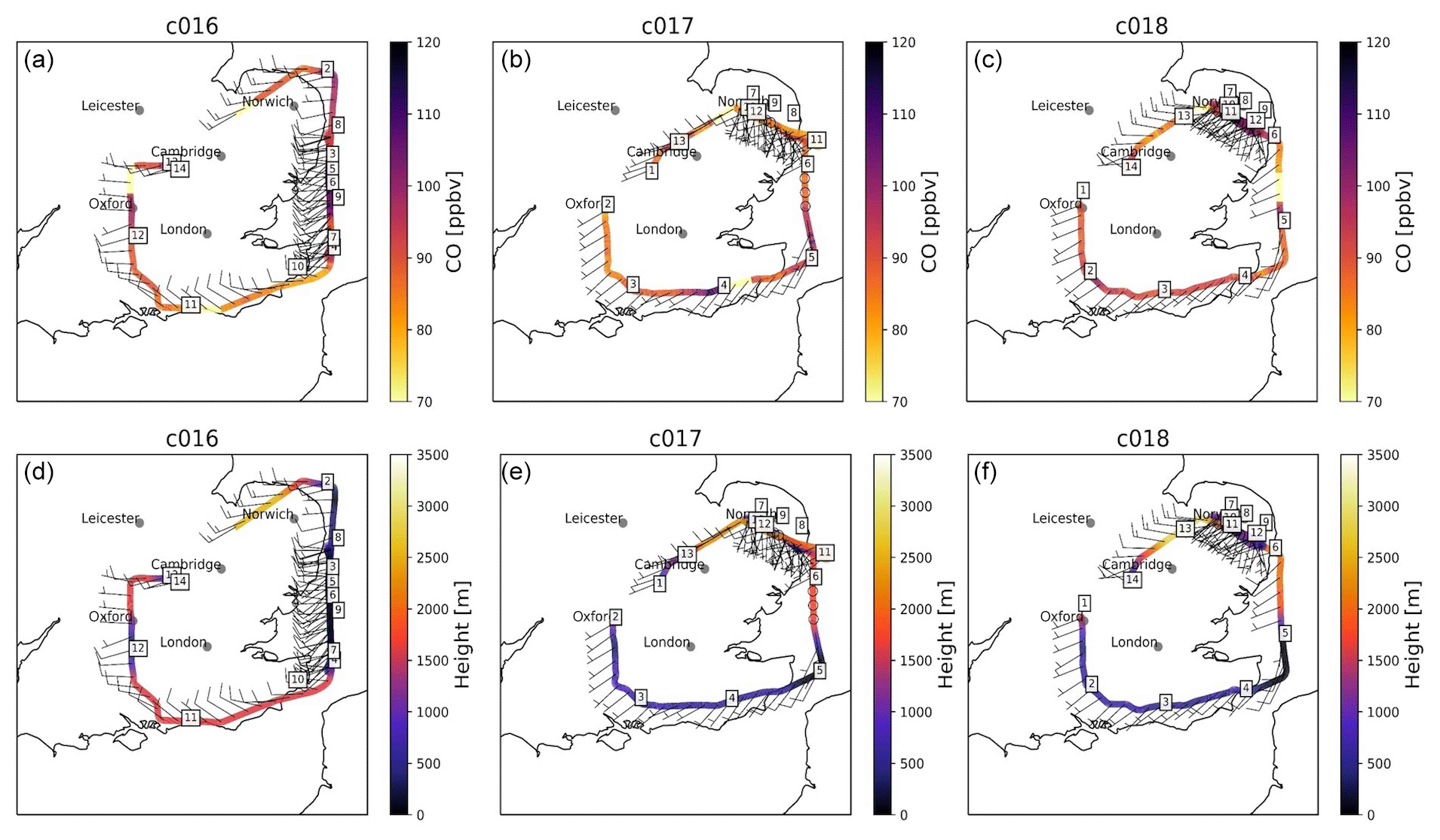
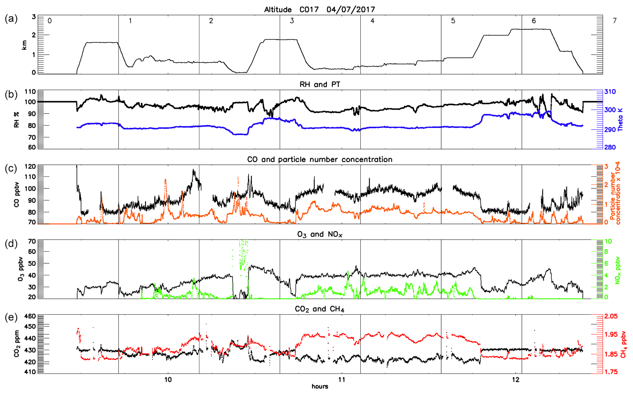
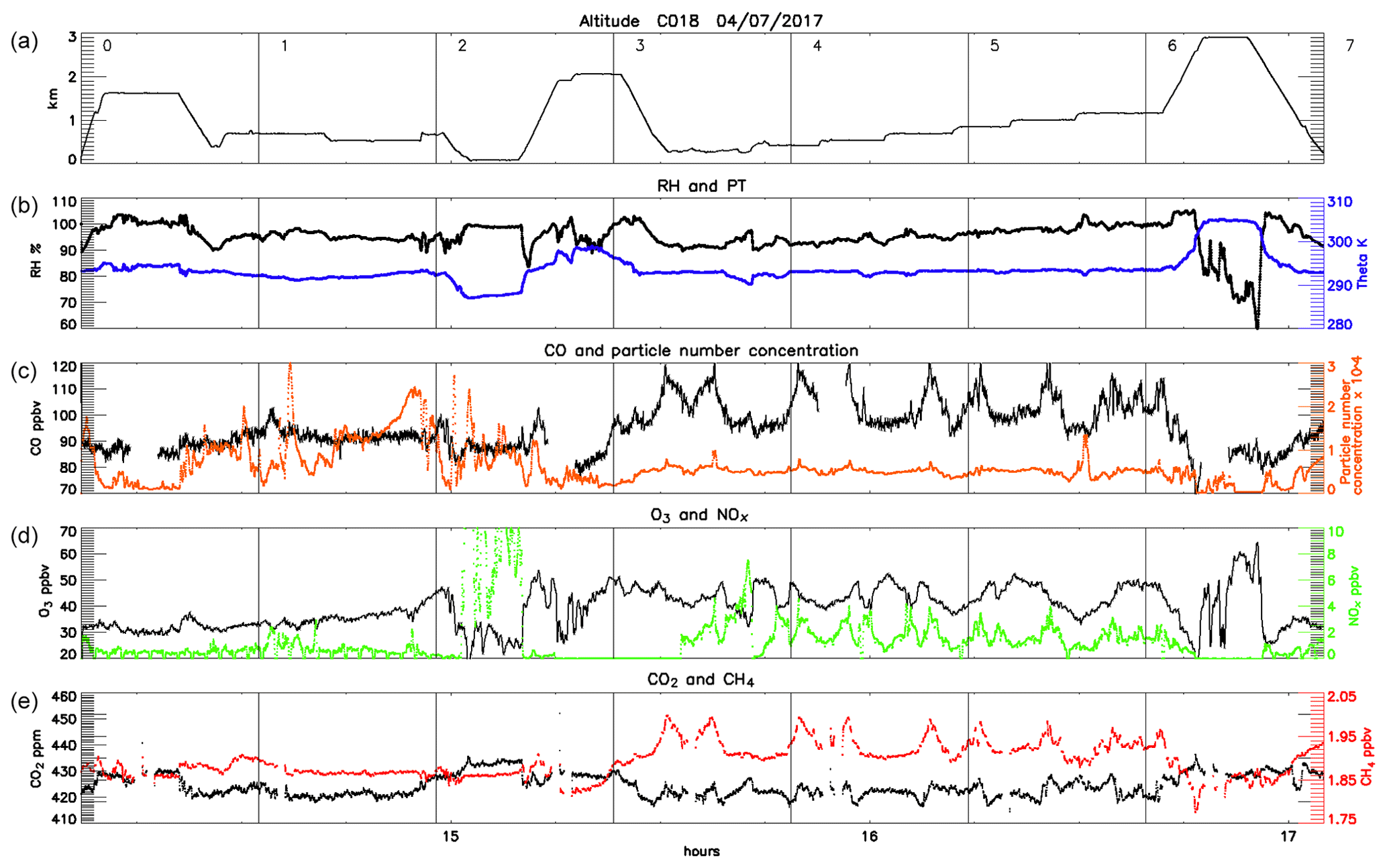
Figure 1 Map of flight paths for all three flights (C016 on Monday 3 July 2017 and C017 and C018 on Tuesday 4 July 2017). Panels (a, b, c) show the concentrations of CO measured on board at (d, e, f) FAAM BAe-146 altitude. Arrows indicate wind speed and direction at 1 min intervals along the path. The numbers in boxes correspond to distinct flight segments which are used hereafter to locate FAAM BAe-146 geographically during the flight.

Due to the change in the synoptic situation between the two flight days, we observed two very different patterns of pollution. Consistent westerly winds on 3 July gave rise to a distinct “plume” east of London over the Thames Estuary, with elevated gas and particle concentrations relative to the upwind air west of London. The clear definition of the plume edges allowed us to quantify the outflow of pollution from London and estimate emissions of CO₂, CO and CH₄ from the city (see Sect.  3.3.3). Relatively stagnant conditions coupled with a shift in wind direction on 4 July reduced the influence of London emissions on the surrounding region. High pollutant levels measured during flights C017 and C018 were thus more easily attributed to local sources (see Sect. 3.3).

2.2 Sampling platform

The UK's Facility for Airborne Atmospheric Measurements (FAAM) BAe-146-301 atmospheric research aircraft (hereafter “FAAM BAe-146” or “the aircraft) provided the airborne science platform. The aircraft has a working altitude range of 100 to 30 000 ft (30.5 m to 9144 m; Petersen and Renfrew, 2009) and a core instrument payload that has been described in full elsewhere (e.g. Harris et al., 2017). The instruments relevant to the current series of flights are described below.

2.2.1 Meteorological measurements

Temperature, wind vector, pressure and humidity are all core measurements on board the FAAM BAe-146. Temperature was recorded with an accuracy of ±0.3 K using Rosemount (Rosemount Aerospace Ltd, UK) type 102 de-iced (Rosemount 102BL) and non-de-iced (Rosemount 102AL) total air temperature sensors (Petersen and Renfrew, 2009; Harris et al., 2017). Pressure and 3-D wind vectors were recorded with estimated uncertainties of 0.3 hPa and 0.2 ms⁻¹ respectively (O'Shea, 2014b; Allen et al., 2011). Humidity was measured only in cloud-free air with a General Eastern 1011B chilled mirror hygrometer. Altitude, position and aircraft velocity data were recorded at 32 Hz by a GPS-aided inertial navigation system. The measurement protocol for these and other atmospheric parameters has been described in detail by Petersen and Renfrew (2009) and Allen et al. (2011).

2.2.2 Trace gas concentrations

Volatile organic compounds (VOCs) were sampled using the whole-air sampling (WAS) system fitted to the rear hold of the FAAM BAe-146. The system consists of 64 silica passivated stainless-steel canisters (Thames Restek, Saunderton, UK) connected via a 3∕8 in. diameter stainless-steel sample line to an all-stainless-steel assembly metal bellows pump (Senior Aerospace, USA) which draws air from the port-side sampling manifold and pressurised air into 3 L canisters (to a maximum pressure of 3.25 bar giving a useable analysis volume of up to 9 L). The collection time of ∼20 s equates to a smoothed average VOC concentration over ∼2 km (Lee et al., 2018). The WAS canisters were analysed by withdrawing and drying 700 mL samples of air using a glass condensation finger held at −40 ^∘C. These samples were pre-concentrated using a Markes UNITY 2 pre-concentrator (fitted with an ozone precursor adsorbent trap) and CIA Advantage autosampler (Markes International Ltd) and then transferred to the gas chromatograph (GC) oven for analysis as described by Hopkins et al. (2011). Further details are given by Lewis et al. (2013) and Lidster et al. (2014).

In situ measurements of NO were made using a custom-built chemiluminescence instrument (Air Quality Design, Inc.) with NO₂ measured by photolytic conversion to NO on a second channel. In-flight calibrations were carried out above the boundary layer at the beginning and end of each flight by adding a small flow of 5 ppmv NO in nitrogen (The BOC Group plc) to the sample inlet. The NO₂ conversion efficiency was measured using gas-phase titration of the NO by O₃ in the calibration to NO₂. The calibration factors were interpolated throughout the flight to account for any sensitivity drifts in the instrument. Detection limits are ∼22 pptv for NO and ∼23 pptv for NO₂ for 1 Hz averaged data, with estimated accuracies of 15 % for NO at 0.1 ppbv and 20 % for NO₂ at 0.1 ppbv.

Continuous 1 Hz measurements of CO₂ and CH₄ were made by the Fast Greenhouse Gas Analyser (FGGA; model RMT-200, Los Gatos Research, USA). The instrument was calibrated roughly hourly using a two-point calibration by sampling two cylinders of air containing CO₂ and CH₄ at mole fractions that span the normal measurement range. A third “target” cylinder containing intermediate mole fractions of CO₂ and CH₄ was sampled approximately midway between hourly calibrations to allow for an assessment of the calibrated data quality. During 12 flights conducted between May and July 2017, the average difference between the target cylinder measurements and the known cylinder composition was −0.047 ppmv for CO₂ and −0.49 ppbv for CH₄. The standard deviation of this difference at 1 Hz was 0.348 ppmv and 1.64 ppbv respectively. Combining these with the uncertainties associated with water vapour correction (0.150 ppmv and 1.03 ppbv respectively) and the certification of the target cylinder (0.075 ppmv and 0.76 ppbv respectively) yields nominal total uncertainties of 0.386 ppmv for CO₂ and 2.08 ppbv for CH₄ at 1 Hz. A detailed description of the in-flight calibration system is given by O'Shea et al. (2013).

Measurements of CO were made with a fast-response vacuum-UV resonance fluorescence spectrometer with an uncertainty of 2 % (model AL5002, Aero-Laser GmbH, Germany; Gerbig et al. 1999). Ozone (O₃) concentrations were measured using a UV photometric analyser (model TEi-49i, Thermo Fisher Scientific Inc., USA).

All trace gas concentrations from the on-board instrumentation are reported as molar (volume) concentrations.

2.2.3 Aerosols

Submicron non-refractory aerosol composition was measured by an Aerodyne Research (Billerica, MA, USA) compact time-of-flight aerosol mass spectrometer (CTOF AMS) (Canagaratna et al., 2007; Drewnick et al., 2005) following the sampling strategy described in previous studies (Crosier et al., 2007; Capes et al., 2008; Morgan et al., 2009). The measurement accuracy is estimated to be 10 % (not considering the collection efficiency uncertainty), and the limits of detection are ∼40 ng m⁻³ for organics and ammonium and ∼5 ng m⁻³ for nitrate and sulfate (Drewnick et al., 2005). Ionisation efficiency of nitrate and relative ionisation efficiencies of ammonium and sulfate were obtained from calibrations performed using monodisperse ammonium nitrate and ammonium sulfate (see Robinson et al., 2011, and Morgan et al., 2010). Concentration of ultrafine aerosol was monitored using a condensation particle counter (CPC; model 3786, TSI Incorporated, MN, USA) at 1 Hz, while an additional optical particle counter (OPC; Grimm Aerosol Technik Ainring GmbH & Co. KG, Germany) was used to correctly count and size aerosol particles (Allen et al., 2011). Aerosol scattering at 450, 550 and 700 nm was recorded using a three-channel TSI 3563 integrating nephelometer.

2.3 Air mass transport

We make use of the FLEXPART Lagrangian particle dispersion model (Stohl et al., 2013, and references therein) adapted for WRF (Brioude et al., 2013a, b) to characterise air mass transport conditions during the STANCO campaign. Meteorological input from WRF is provided with a 1-hourly time step at a spatial resolution of 3 km × 3 km. Clusters of 500 back-trajectories are computed back in time for 24 h at 1 h intervals.

The output is a gridded “footprint emissions sensitivity” of the retroplume (as described in Stohl et al., 2007). It quantifies the residence time of the back-trajectory plume over each grid cell and, hence, its potential contribution to the air mass composition at the point of the trajectory's release. As we were looking for correspondences with ground-level emission sources, we select only the back-trajectories from below the boundary layer, as interpolated by FLEXPART from the WRF simulations.

3 Results

3.1 Meteorology and air mass history

Meteorological conditions on 3–4 July 2017 are summarised in Figs. 1 and 2 which show the low-level wind fields and vertical soundings of temperature and wind respectively.

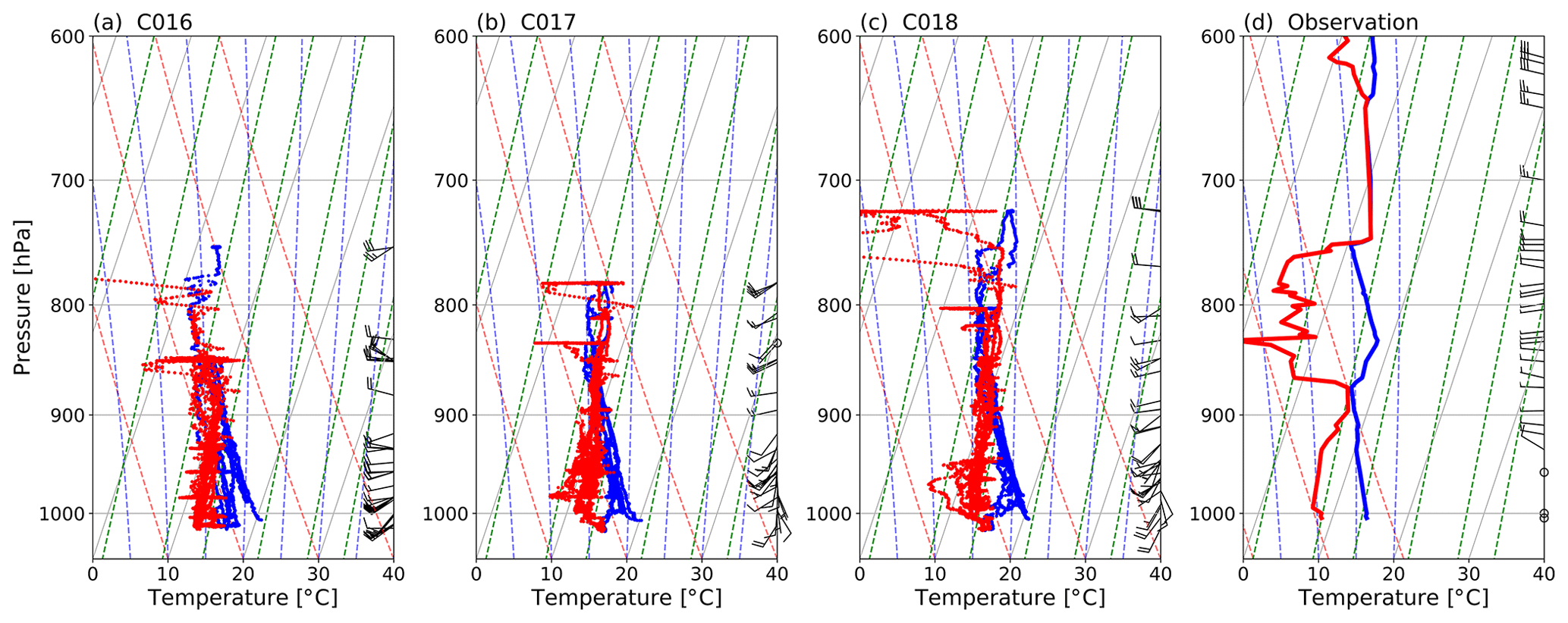
Figure 2 Skew-T log-P plots showing (a–c) temperature (blue) and dew point temperature (red) for all three flights and (d) temperature and potential temperature from a radiosonde launched from Nottingham at 00:00 UTC on 4 July 2017.

During C016 (3 July) the mean flow was mainly westerly with winds <15 m s⁻¹ across the London area, giving favourable conditions to study the London plume (see Sect. 3.2.1 for further details). There was sun in the east flight quadrant and clouds and slight precipitation in the south-west. The high-pressure system that brought westerly flow on 3 July moved north overnight, bringing south-westerlies for both flights on 4 July. Wind speeds also dropped to <10 m s⁻¹, and urban air pollution was dispersed rather than concentrated into a plume.

The Skew-T log-P diagrams in Fig. 2 show that the lifted condensation level was ∼890 hPa, effectively constraining pollution from near-surface emissions below this height. Figure 2a–c show the height of the mixed layer varied between ∼800 m (during flight C016 on 3 July) and ∼1500 m (during C018, the afternoon flight on 4 July). Our airborne observations show good agreement of mixing depth with those obtained from a radiosonde ascent over nearby Nottingham at 00:00 UTC on 4 July (Fig. 2d). Those sounding profiles indicate that all airborne sampling was performed within the mixed layer.

3.2 Airborne observations

Figure 1 shows the path of the FAAM BAe-146 during each of the three flights, broken into segments of equal duration, which are numbered for ease of reference. It should be noted that due to the change in wind direction between the 2 d, C016 flew in a clockwise direction whereas the two flights on 4 July circled anticlockwise. Time series of aircraft altitude and continuously measured gas-phase concentrations and particle number concentration are plotted for each flight in Figs. 4–6. The numbers shown in panel (a) of each correspond to the numbered flight segments in Fig. 1 to enable us to interpret the observed features geographically.

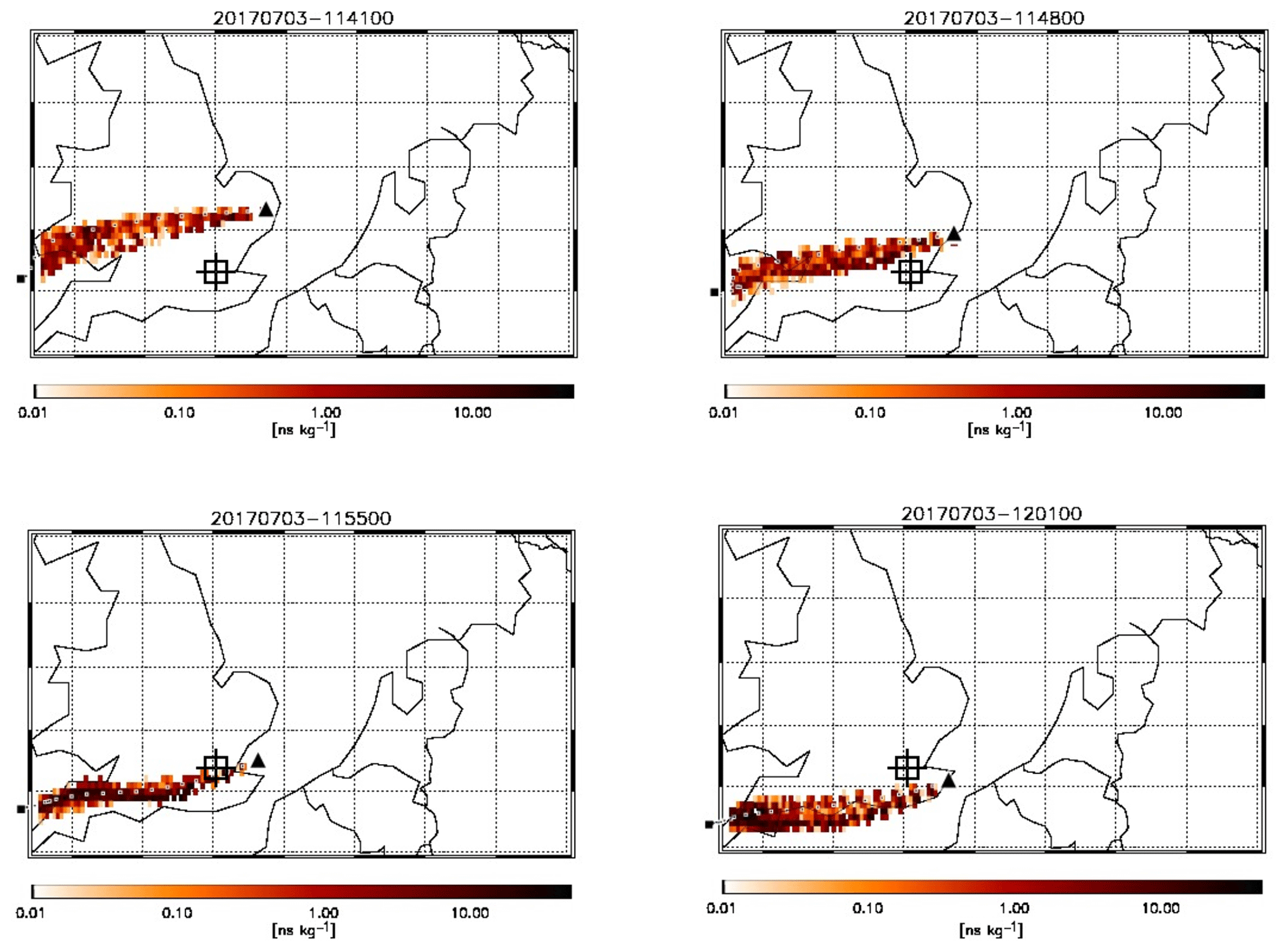
Figure 3 FLEXPART modelled footprint of air mass arriving at the location of FAAM BAe-146 (black triangles) at four different positions along the reciprocal runs of flight C016. Each coloured pixel indicates the relative contribution of an inert tracer in that air to the total concentration of that tracer sampled on board. The large black square shows the point of release of the air 24 h prior to being intercepted by the aircraft. The dotted line of black and white squares shows the hourly weighted average trajectory of the air mass based on the relative contributions shown. The square target indicates the approximate position of central London.

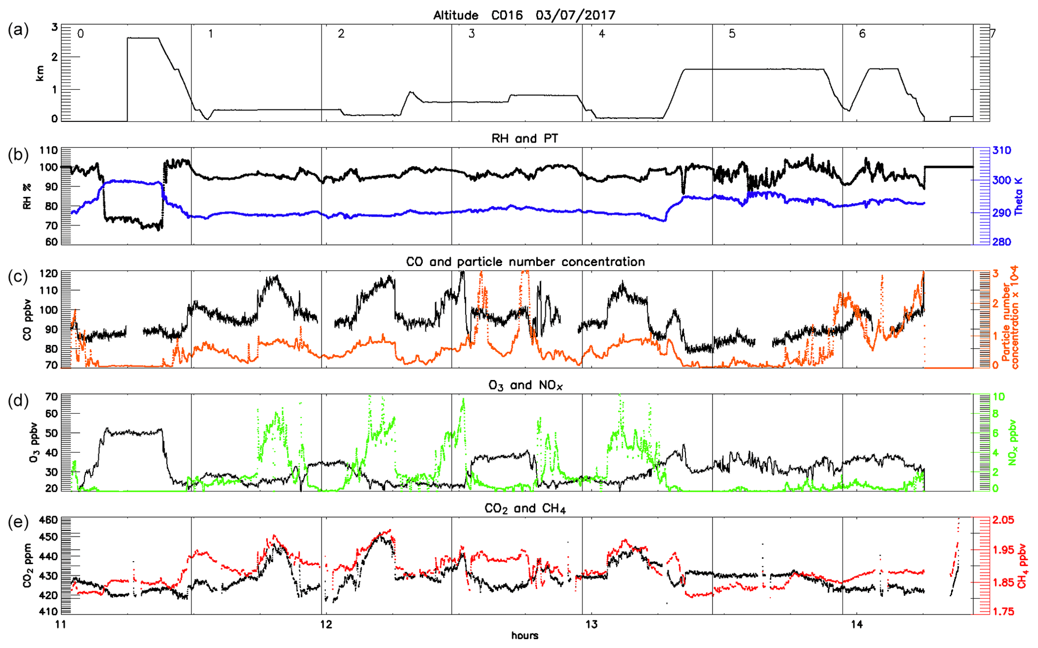
Figure 4 Time series of the main observations during the first flight (3 July, late morning) showing the altitude of the aircraft (a), relative humidity (b, black) and potential temperature (blue), CO concentration (c, black) and particle number concentration (orange), O₃ (d, black) and NO_x (green) concentrations, and CO₂ (e, black) and CH₄ (red) concentrations. The numbered vertical lines correspond to the numbers along the flight path shown in Fig. 1.

Figure 5 As in Fig. 4 but for the second flight (C017; 4 July, morning).

Figure 6 As in Fig. 4 but for the third flight (C018; 4 July, afternoon).

In addition to the suite of real-time continuous measurements sampled from the aircraft, 24, 14 and 24 WAS measurements were collected during each flight respectively and subsequently analysed for VOC concentrations. Table 1 shows average particle number concentration and concentrations of all trace gases for the whole flight, the background (upwind of London) flight segments and the plume (downwind of London) flight legs closest in altitude to the upwind segment(s) for each of C016–C018. It should be noted that as WAS was manually initiated in response to observed elevations in other trace gases as well as during targeted flight segments up- and downwind of London, the data must be considered skewed to more polluted locations. A further caveat when interpreting these data is the small sample size.

Table 1 Average concentrations of trace gases (ppbv) and particle number concentration (particulate matter, PM; cm⁻³) for the whole flight, upwind segment and downwind reciprocal runs at an altitude corresponding to the upwind leg for each flight. Numbers in parentheses show ±1 SD.

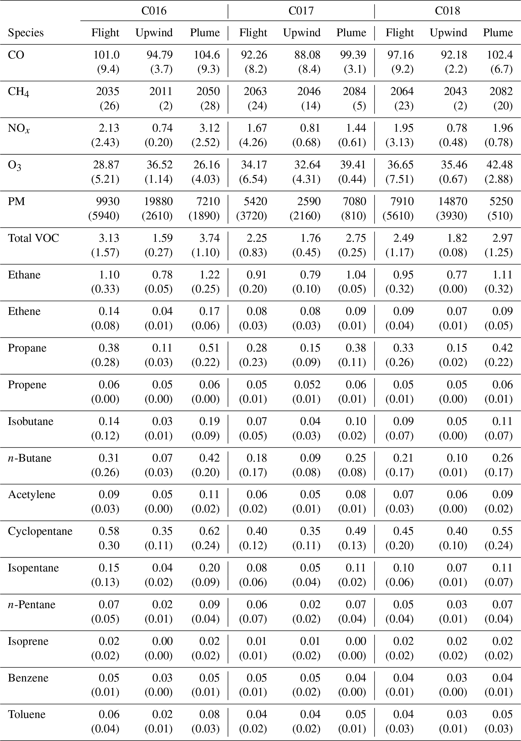
Figures 4–6 and Table 1 show the clear enhancement in gas-phase concentrations downwind of London during all three flights. CO concentrations are as low as ∼88–95 ppbv on the upwind flight segments but increase by ∼10 ppbv in the plume on each flight. Enhancements of CH₄ are around 20 % in all downwind plumes (rising from ∼2.01–2.05 to ∼2.05–2.08 ppmv). NO_x reached peaks of >14 ppbv on 3 July and >4.5 ppbv on 4 July downwind of London compared to levels between ∼0.7 and 0.8 ppbv in the relatively clean upwind air. NO_x concentrations were highly variable across all three flights as expected for such short-lived species associated with fresh local emissions. Total VOC concentrations rose by a factor of ∼2 (from ∼1.6–1.8 to ∼2.7–3.7 ppbv), although the changes in individual species varied between the flights. The only exception to this pattern is ozone, a secondary pollutant formed by photochemical reactions over a matter of hours and which is destroyed by direct reaction with NO (referred to as NO titration). O₃ levels were considerably lower in the plume (∼26 ppbv) than along the upwind flight segment (36.5 ppbv) in flight C016, pointing to strong NO_x sources in London. All three flights had similar concentrations of O₃ upwind of London (∼32.6–36.5 ppbv), leading to high O₃:NO_x ratios. This is characteristic of aged air masses and suggests that the pollution encountered along the upwind flight segments to the west (C016) and south-west (C017 and C018) of London is the result of transported rather than local fresh emissions. This is discussed in further detail below.

The other striking difference between the flights, also symptomatic of the origin of the transported air, is the particle number concentration. Both C016 and C018 encountered much higher aerosol counts upwind than in the London outflow (2×10⁴ and 1.5×10⁴ cm⁻³ vs. 7×10³ and 5×10³ cm⁻³ respectively); in both cases, this background air had travelled from the west to south-west. By contrast, flight C017 sampled air transported from the west to north-west of the UK, and particle number concentration was lower upwind of London (2.5×10³ vs. 7×10³ cm⁻³ downwind), suggesting the enhancement was due to a strong source SW of London rather than emissions local to the flight track.

3.2.1 Flight C016: westerly advection

A large part of C016 took place to the east of the UK coast, flying mostly below 800 m altitude over the sea, where we sampled air inside the planetary boundary layer (PBL) in conditions of high RH (values between 90 % and 100 %) and a potential temperature of ∼290 K. Pollutant levels during this flight were higher than the two other (inland) flights. The enhancement in the trace gas and particle number concentrations can be almost entirely attributed to pollutants emitted and advected from the UK with little influence of continental Europe. Air mass back-trajectories for the flight segments to the east of London are shown in Fig. 5. The sharp edges to the plume can be deduced from these snapshots in time, with the air masses intercepted at 11:48:00 and 11:55:00 traversing London but those at 11:41:00 and 12:01:00 bypassing the city and bringing cleaner air from other regions. In this downwind section of the flight (2–9 of Fig. 4 and Fig. 1a) CO concentrations ranged from 90 to 120 ppbv. We also observed the highest values of NO_x, often in excess of 10 ppbv and peaking at 14.6 ppbv, and concentrations of up to 450 ppmv of CO₂ and up to 2 ppbv of CH₄. Particle number concentration was mostly <10⁴ cm⁻³, with the exception of two layers between 600 and 700 m altitude where numbers peaked at 3×10⁴ cm⁻³ east of and parallel to London (segments 6–7). Above the mixed layer and at higher altitudes >1500 m we did not observe any striking pollution features.

3.2.2 Flights C017–C018: south-westerly advection

Meteorological conditions were more quiescent on Tuesday 4 July with relatively slack air flow from the WSW to WNW throughout the day, giving way to some localised re-circulation, particularly to the north-east of London (the origin and transport of air masses are discussed in more detail in Sect. 3.3). We did not encounter a clear London plume, but instead we were able to identify other more local pollution events which are presented in Sect. 3.3.

Flights C017 and C018 followed the same flight plan and altitudes as far as possible, as shown in Figs. 1 and 4–5. The initial altitude was 1500 m during both flights, before a descent to 700 m to the west and south of London and then to 25 m over the Dover Strait and English Channel (flight segments 4–5 in Figs. 5 and 6) where we were able to sample distinct plumes from marine traffic (see Sect. 3.3.2). There then followed the series of reciprocal runs over East Anglia (segments 6–11) where a diffuse plume of pollution was encountered with elevated CO and CH₄ and, to a lesser extent, particle number concentrations over a relatively large area. Within this, two distinct plumes of pollution were observed and sampled in both flights – an interesting case of transport from two distinct outflow plumes which is analysed in more detail in Sect. 3.3.4.

The humidity and temperature during these flights were similar to those during C016, with RH varying between 95 % and 100 % and potential temperatures between 290 and 295 K. However, conditions during C017 and C018 differed in several notable ways. The morning flight (C017) was characterised by relatively stagnant winds (see Figs. 1 and 2) and a low mixed-layer height (∼800 m). Pollutant concentrations were the lowest sampled (Fig. 5). During the afternoon, wind speed increased, the height of the PBL rose to ∼1500 m and the wind direction became more south-westerly, leading to distinct differences between the composition of the upwind samples during the two flights.

Upwind measurements from flight C017 showed very low levels of CO, O₃ and particles (mostly <88 ppbv, <35 ppbv, <2500 cm⁻³ with periodic transient elevated concentrations) compared with flight C016, indicating much cleaner background air. NO_x levels were slightly higher though (mostly ∼1.0 ppbv with multiple peaks above 2.5 ppbv), suggesting a larger relative contribution from local emission sources than on the previous day. This fresh NO_x likely also contributed to the reduced O₃ concentrations through NO titration. The total concentrations of VOCs from the four WAS measurements collected along this segment correlate well with other pollutants (r²=0.85, 0.99, 0.84 and 0.79 against CO, NO_x, CH₄ and particle number concentration respectively). However acetylene, which has an atmospheric lifetime of ∼2–3 months compared with a typical OH concentration of $\sim {\mathrm{10}}^{-\mathrm{6}}$ molec. cm⁻³, is not well correlated with NO_x (r²=0.48), although it is with the longer-lived pollutants (r²=0.92, 0.88 and 0.74 against CO, CH₄ and particle number concentration). This is typical of transported air (McMeeking et al., 2012), further confirmation that we were sampling aged background air mixed with some local fresh emissions. Back-trajectories (Fig. 11a, b) show winds were blowing from the west and north during flight C017, bringing relatively clean air to the region. This is further corroborated by a high-altitude leg during the reciprocal runs over East Anglia (flight segment 12 in Figs. 1 and 5) downwind of London. Along this leg, which at a height of just under 2 km was well above the PBL, concentrations of gas-phase pollutants were all lower than those sampled in the upwind PBL (∼10 pptv of NO_x, CO∼80 ppbv, O₃ ∼26 ppbv), indicating the long-range transport of clean air into the region.

In contrast to the morning flight, the back-trajectories for the afternoon flight, C018 (Fig. 11c, d), show a mix of air mass origins. While a large proportion of the air also arrives from the west and north, there is a substantive contribution from the west-south-west, along a similar trajectory to that for flight C016. This rather neatly explains our upwind atmospheric measurements lying between those of the two other flights, C017 with clean air from north and west and C016 with high CO and particle number concentrations from strong pollution sources to the south-west. NO_x concentrations are elevated along this segment with local sources strongly contributing to the pollution sampled here as would be expected given the slower wind speeds on 4 July. However, similar to C016, particle number concentration reached 2×10⁴ cm⁻³ between flight segments 2 and 4 during C018 (Fig. 6), apparently associated with an air mass originating from SW England as no enhancement was observed during the latter stages of the flight when the air masses were transported from more northern and central regions. This is in sharp contrast to the C017 (<5×10³ cm⁻³ in this area) flight with the difference likely caused by the higher afternoon boundary layer uplifting local particles from southern England. Although the absolute values differed between the two flights, similar patterns were observed in gas-phase and particle number concentrations. Aside from a few specific locations, which are described in Sect. 3.3, little pollution was encountered during either flight, with NO_x generally <2 ppbv, CH₄<1.95 ppbv, CO₂<430 ppmv and particle number concentration <10⁴ cm⁻³.

3.3 Pollution episodes

Each of the three flights followed similar flight paths, circling London just beyond the outer ring road (M25). Small differences in wind speed and direction across the three flights resulted in air masses with very different origins contributing to the background composition and to individual pollution events. We now present four such episodes encountered during one or more of the flights, following the route around London in an anticlockwise direction, reflecting on the similarities and differences in air mass origins and likely sources in each case.

3.3.1 Gatwick area: flight C017, 4 July

During C017, CO concentrations were generally ≪100 ppbv, with the exception of a peak reaching 115 ppbv detected at an altitude of around 500 m to the south of London in the vicinity of Gatwick airport (at 51^∘ N, 0.55^∘ E; close to segment 4 in Figs. 1 and 5). This elevation in CO was associated with an enhancement in NO_x of up to 2 ppbv, suggesting vehicular emissions to be a likely source. This feature was not observed during either flight C016 (Fig. 4) or C018 (Fig. 6).

Figure 7 shows air mass footprints from FLEXPART back-trajectories for the 5 min time interval during which the plume was observed on board C017 and the interval for the same location during the afternoon flight (C018). Although we acknowledge that transport-related emissions are highly time-dependent, these footprints indicate the difference is more likely the result of a greater influence of transported pollution from land-based sources in the morning, with the sampled air spending more time over the sea in the afternoon. The NAEI emission inventory for this area suggests this was most likely local pollution from the Brighton area (population ∼275 000) and the major A26 road.

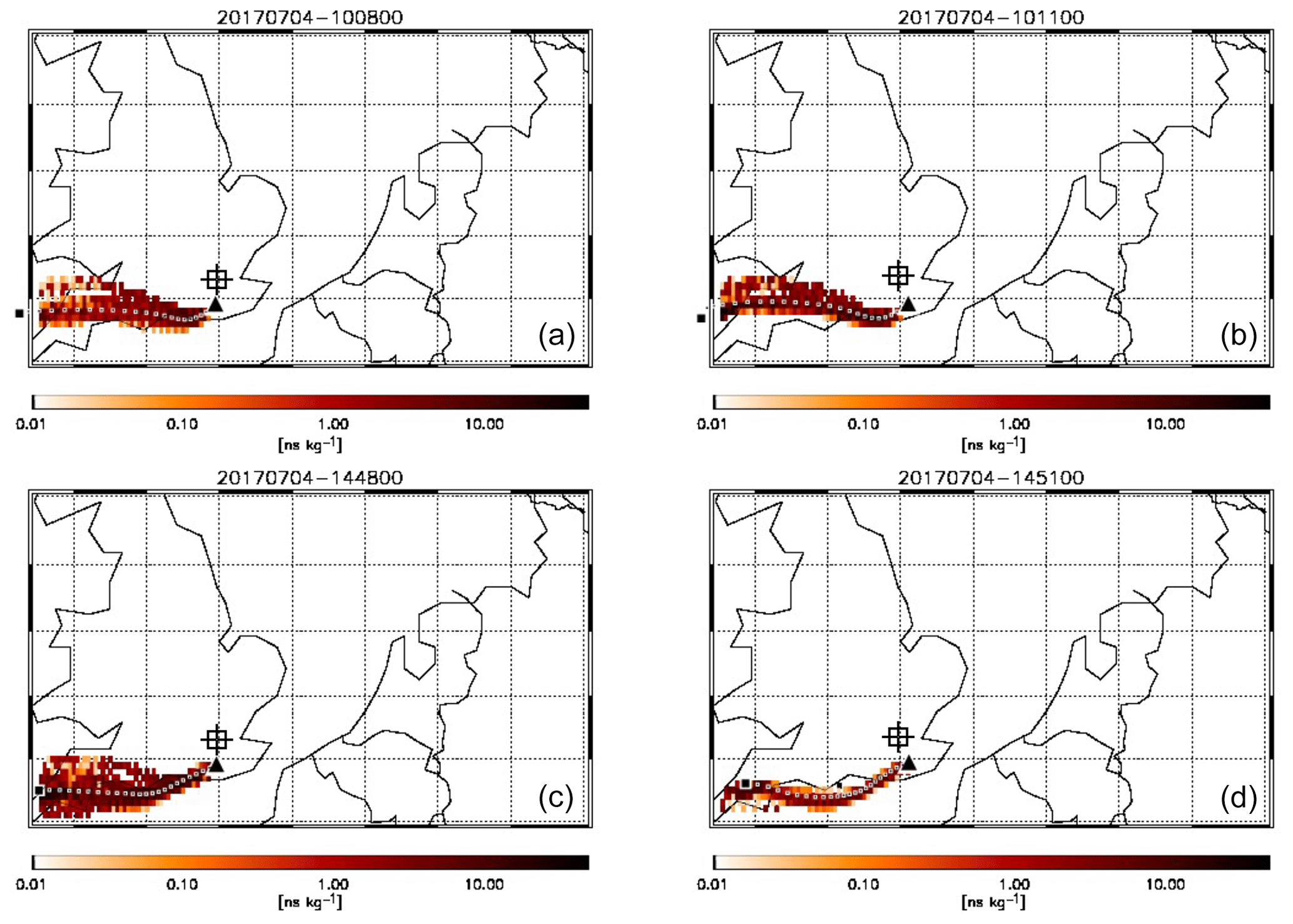
Figure 7 FLEXPART modelled footprint of air mass arriving at the location of FAAM BAe-146 (black triangles) at 10:08 and 10:11 during flight C017 (a, b) and at 14:48 and 14:51 during flight C018. Each coloured pixel indicates the relative contribution of an inert tracer in that air to the total concentration of that tracer sampled on board. The large black square shows the point of release of the air 24 h prior to being intercepted by the aircraft. The dotted line of black and white squares shows the hourly weighted average trajectory of the air mass based on the relative contributions shown. The square target indicates the approximate position of central London.

3.3.2 Marine emission sources

We observed substantial local elevations in concentrations of all pollutants during the low-level flight legs over the Dover Strait and English Channel for all three flights (segments 8, 4–5 and 4 respectively in Figs. 4–6). The smaller sampling footprint associated with low-level flying meant it was easier to positively identify the sources of these pollution events than over the land surface, and we were able to directly attribute some of the peaks to specific vessels. We describe one such situation here.

Between around 10:21 and 10:27 UTC on 4 July (flight C017) we overflew the Dover Strait at an altitude of between 25 and 75 m. Clear enhancements in pollutant concentrations and particle number concentration were directly seen on most on-board instruments and we were able to observe the passage of a number of large ships which appeared to correlate with these enhancements. In order to evaluate whether a part of the observable signal in the different variables was attributable to marine traffic, we plotted the time series of NO_x, NO, NO₂ and CO₂ concentrations and the particle number concentration (Fig. 8). We identified a number of plumes throughout this portion of the flight but focus our analysis on the clear sharply defined peak in concentration observed at 10:22:30 and marked with an “X” in Fig. 9. At this point, NO_x levels were elevated by a factor of ∼20 and particle number concentration by a factor of ∼5 compared with the flight leg as a whole.

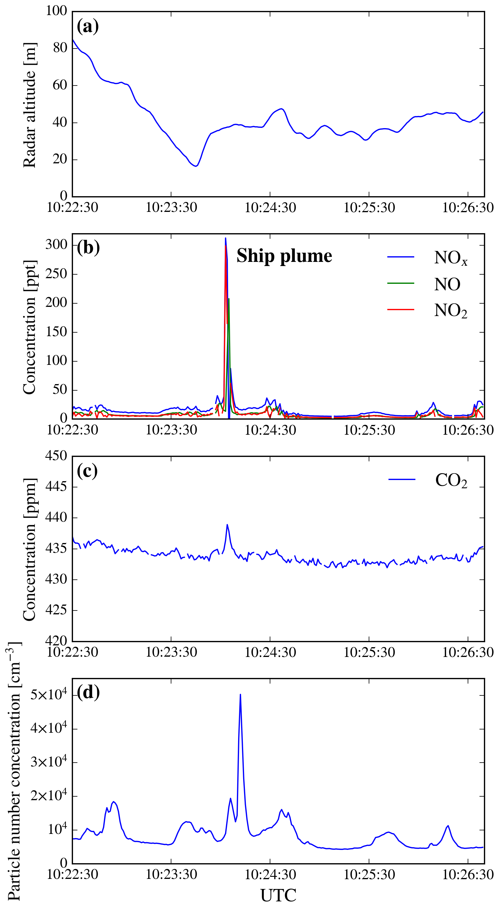
Figure 8 Time series of different variables measured above the sea during the C017 flight: (a) altitude; (b) NO, NO₂ and NO_x concentrations; (c) CO₂ concentration; and (d) total aerosol concentration. Only the times close to the large plume that could be correlated to a specific vessel are shown here. CO and O₃ concentrations (not shown) exhibited no enhancement. The plotted time period corresponds to the beginning of a level run at ∼40 m altitude, the trajectory of which can be seen in Fig. 9.

As marine emissions are known to be an important source of both NO_x and PM (Corbett et al., 1999), we used data obtained from Marine Traffic (https://www.marinetraffic.com, March 2020) to examine the vessels navigating this area at the time of flying over. Figure 9 shows the portion of the flight path above the sea and maps the paths of those ships with a tonnage >10 kt (thin coloured lines, with colour ranging from purple to yellow corresponding to specific times between 10:13:20 and 10:26:40), overlaid with the path of the aircraft (thick line); arrows denote wind speed and direction.

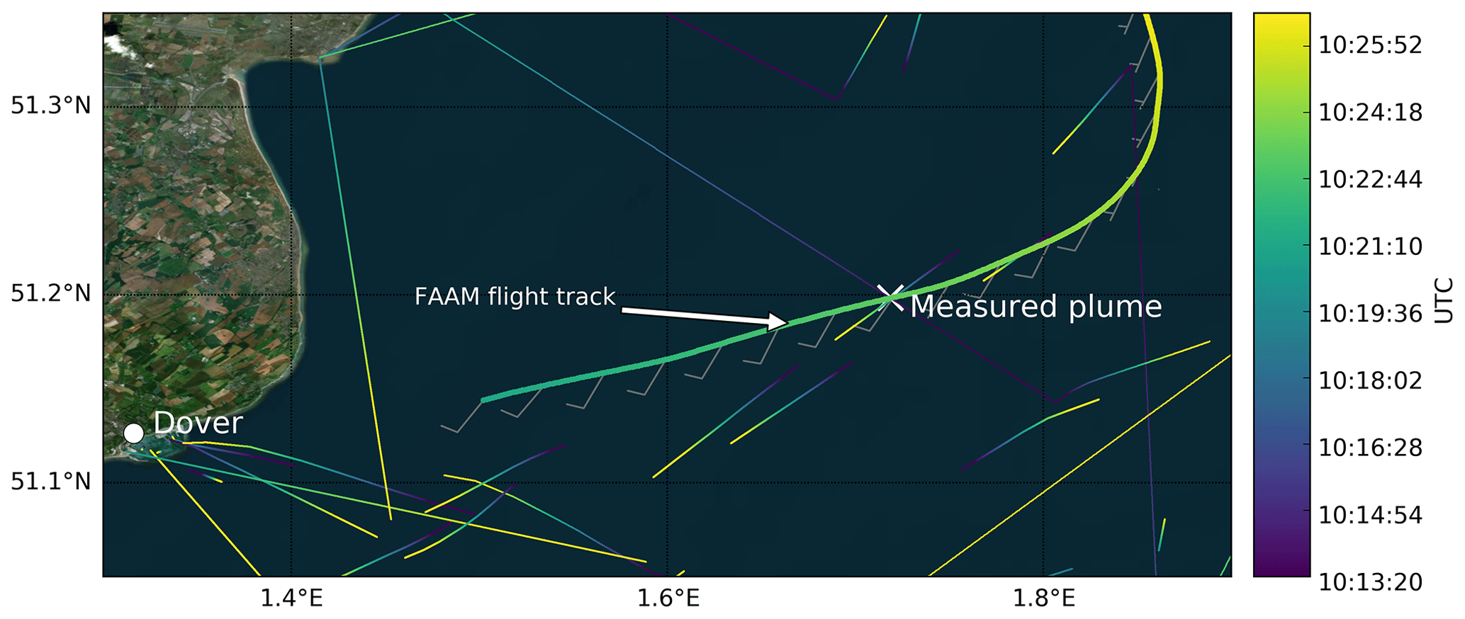
Figure 9 Flight track of FAAM BAe-146 (thick coloured line) during flight C017 at the beginning of the level run at ∼40 m a.m.s.l. where a large ship plume was measured (indicated with a white cross). Wind speed and direction measured by FAAM BAe-146 are shown by the wind barbs. The trajectories of all the ships >10 kt are shown by thin coloured lines with the colour scale denoting time. The base map was created using the World Imagery maps in ArcGIS^® software by Esri. ArcGIS^® and ArcMap™ are the intellectual property of Esri and are used herein under license. Copyright ©Esri. All rights reserved. For more information about Esri^® software, please visit https://www.esri.com (last access: March 2020).

The “X” in Fig. 9 corresponds to the location of the prominent peaks in elevation seen in Fig. 8b–d. At this point, a large ship had passed under the flight path shortly ahead of our transit and we intersected its plume around 40 s later. We were able to positively identify this vessel from Marine Traffic data as a 15 kt Liberian container ship. Other smaller plumes seen during C017 and the other flights could not be directly attributed to a single ship and are likely an accumulation of emissions from a number of smaller or more distant vessels (as observable in Fig. 9).

3.3.3 London plume: flight C016, 3 July

A narrow, well-defined plume of pollution was encountered downwind of London (flight segments 3–9 in Figs. 1 and 4). A series of reciprocal runs was performed in this outflow over the Thames Estuary at altitudes between 100 and 800 m, capturing its vertical profile. In addition to the continuous measurements, 13 WAS measurements were collected during these flight legs. Table 1 shows the average gas-phase pollutant and particle number concentrations across segments 4, 6 and 7 where the average altitude was ∼450 m. Flight segment 12 in Figs. 1 and 4 lies directly upwind of the city and provided a contrasting relatively clean air mass (evident in Table 1). Five WAS measurements were collected along this leg at an altitude of 550 m.

The outflow from London is easily identified by the substantial and distinct enhancements in NO_x, CO, CO₂ and CH₄ concentrations seen in segments 3–9 in Fig. 4. These are anticorrelated with O₃ concentrations which decreased sharply (to ∼22–25 ppbv) in the plume due to NO titration and are highest (∼35–40 ppbv) in the upwind air mass due to the formation of O₃ and other secondary pollutants from photochemical ageing of more distant emission sources. Total (measured) VOC concentration was also elevated in the plume (peaking at 5.9 ppbv) compared with upwind air (max 1.8 ppbv). However, proportions of longer-lived compounds (e.g. ethane and propane) were higher upwind (∼0.5 vs. ∼0.3 and 0.35 vs. 0.17 ppbv) as were the ratios of benzene to toluene (B:T; 1.78 vs. 0.63) and O₃:NO_x (49.6 vs. 8.4). These are characteristic of decayed urban plumes (McMeeking et al., 2012) and further reinforce that the upwind air mass is more aged. This is also evident in the ratios of benzene to acetylene, another key marker of aged air, which fell from ∼0.7 upwind to ∼0.4 downwind. It should be noted that our value of 0.4 is slightly higher than has been previously reported for London outflow (Parrish et al., 2009; McMeeking et al., 2012; von Schneidemesser et al., 2010) and in conjunction with sampling during flights C017 and C018 suggests that there are strong local sources of benzene to the east and north-east of the city.

Figure 10 shows the concentrations of key VOCs for each reciprocal run in the plume (flight segments 3–7 in Figs. 1 and 4); the altitude of each is indicated on the y axis. The highest absolute concentrations occurred at altitudes between ∼200 and 600 m. This is suggestive of pollution being lofted above a layer of cooler surface air outside of the urban heat island, i.e. the urban boundary layer phenomenon. Overall, our observations support the conclusion that it was London outflow that we sampled during the reciprocal runs over the Thames Estuary, with little evidence of substantial contributions from local emission sources. The relatively strong (>15 m s⁻¹) prevailing south-westerly wind ensured on-board measurements provided a sufficiently clear plume and sufficiently large data footprint to allow the calculation of regional-scale CO, CO₂ and CH₄ fluxes. While measurements are vertically discrete and only sample a small percentage of the vertical profile, the high temporal and horizontal resolution of the sampling of the plume allowed for the data to be interpolated across the full altitude range of the observations.

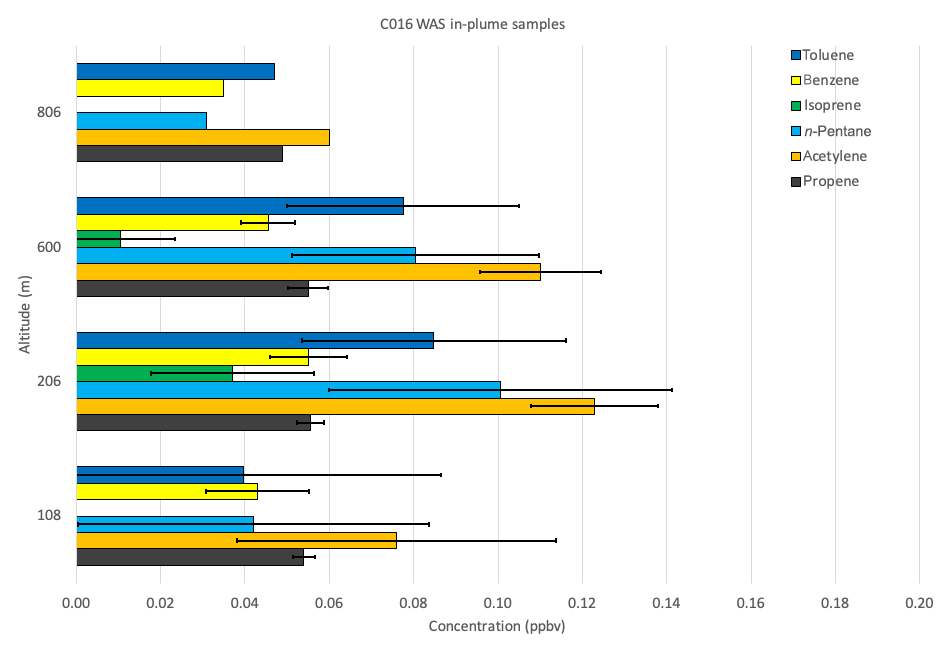
Figure 10 Average concentrations of key VOCs (ppbv) collected via WAS during individual flight legs within the plume detected during flight C016. The average altitude of each flight leg is shown on the y axis. Error bars denote ±1 SD.

Several secondary plumes from shipping emissions were removed from the dataset before pollutant fluxes were calculated. Discrete data points from five horizonal flight legs spanning ∼30–800 m above sea level were interpolated onto a 19×19 grid consisting of 8412 m by 38 m grid boxes in the horizontal and vertical respectively. As the lowest leg of the flight fell within the lowest boxes on the interpolation grid, further extrapolation towards the surface was unnecessary. We assumed that air below the lowest flight track was well mixed and that this track is therefore representative of it and that the full vertical profile of the plume was captured by these flight legs. Boundary layer height was estimated from temperature–humidity profiles to be between 800 and 1000 m while the plume was being sampled. Vertical profiles for NO_x only showed significant enhancement below these heights, indicating a lack of mixing into the free troposphere. NO_x was used to indicate this, as its shorter lifetime leads to near-zero concentrations above the boundary layer, whereas the difference is less pronounced in the longer-lived species such as CO, CO₂ and CH₄.

A vertical plane for the downwind plume was produced, along with the wind vector perpendicular to these planes, using the methodology described by Kitanidis (1997) and Mays et al. (2009). Vertical background runs were created by linearly interpolating between the northern- and southernmost data outside of the plume for each run. These were then transformed using kriging to produce corresponding 19×19 grid boxes for the background planes. Kriging was achieved using the MATLAB “EasyKrig3.0” program (Chu, 2004).

Concentration data were converted point-wise from parts per billion by volume to milligrams per cubic metre using in situ pressure and temperature data. The total flux could thus be calculated for species S, where S is CO, CO₂ or CH₄, using Eq. (1):

$$\begin{array}{}\text{(1)}& \mathrm{flux}={\int }_{\mathrm{0}}^z{\int }_A^B\left({\mathrm{S}}_{ij}-{\mathrm{S}}_{\mathrm{0}}\right)U_{\perp ij}\mathrm{d}x\mathrm{d}z,\end{array}$$

where S_ij is the mole fraction of species S for coordinates in the downwind vertical plane, AB is the background vertical plane and S₀ the mole fraction of S on that plane, and U_⊥ij is the vertical plane of the wind vector perpendicular to the aircraft. The flux is then integrated for altitudes of 0 m to z m, here the top of the plume at ∼900 m.

CH₄, CO₂ and CO fluxes (Table 2) can be compared to a previous study by O'Shea et al. (2014a), who used a similar approach to estimate pollutant emissions. The CO fluxes from London during flight C016 are estimated to be ∼ half those for the summer of 2012, whereas the CH₄ flux here is double that calculated by O'Shea et al. (2014b). Our CO₂ flux estimate, however, falls within the combined uncertainty of O'Shea's. When considering these data, one should be mindful that aircraft measurements are representative of a single point in time and therefore cannot be aggregated over longer periods. As such they are highly sensitive to meteorology and hence emissions footprint and source strength at the time of measurement. In both studies, estimates are based on the measurements of a single flight. Due to the short duration of sampling and significant separation in time between studies, variation in emissions from London (diurnally, seasonally or longer-term) are likely to be substantial and this should be borne in mind when comparing estimated fluxes between studies, although differences in methodology may also contribute to the differences. For a meaningful analysis of patterns and trends in London emissions and a top-down constraint of the NAEI emissions inventory, plumes would need to be repeatedly sampled from aircraft during different seasons, times and locations relative to the pollution source.

Table 2 Emission fluxes from Greater London determined in this study and compared to those found using similar approaches by O'Shea et al. (2014a) and Pitt et al. (2019).

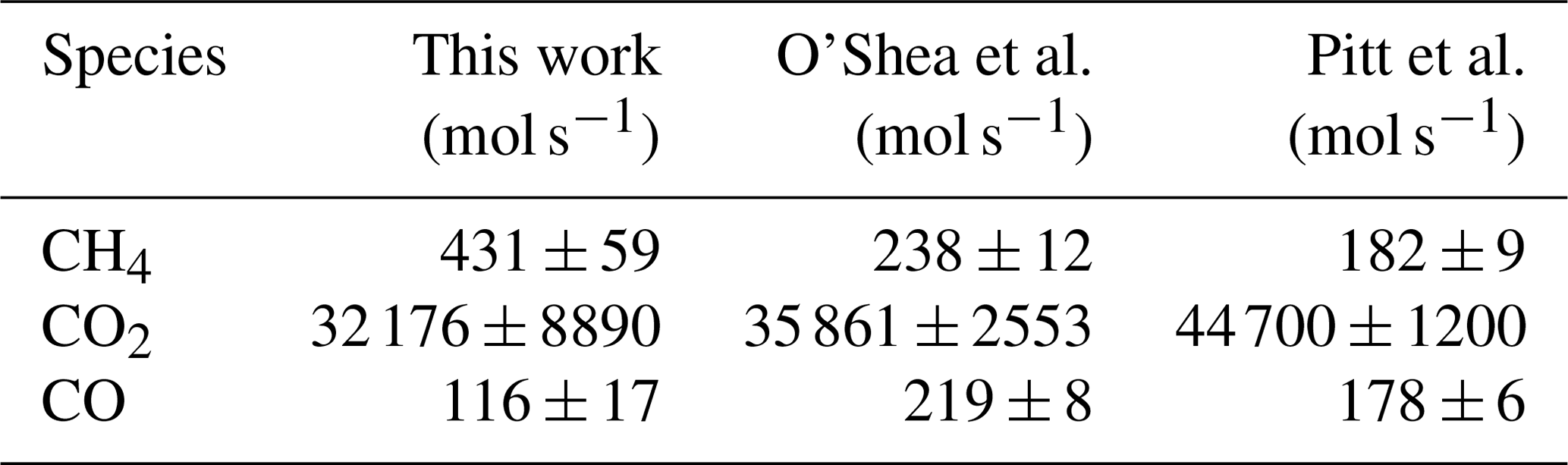
Of particular methodological importance to this approach are the criteria used to define the background air. The impact of this choice in determining which emission sources contribute to the measured fluxes has been the subject of a recent study based on the INFLUX project (Turnbull et al., 2018). In the case of flight C016, due to the evolution of the boundary layer during the times between the upwind and downwind legs, while upwind measurements were evidently sampling clean background (regional) air, we did not consider them representative of the downwind background. Instead, measurements from the downwind leg but outside of the plume were used (following Turnbull et al., 2018). This is a different approach to the upwind background used by O'Shea et al. (2014a), and therefore the measured fluxes correspond to aggregate emissions from different areas. This could in part explain the discrepancy in estimates between the two studies.

The difficulty in defining an emission aggregation area for flights around London for any choice of background criteria has been discussed in depth by Pitt et al. (2019). In their study, fluxes from a different case study flight around London (conducted in 2016) were found to be biased high compared to the results of a simple transport model inversion using the same aircraft data, if the fluxes were assumed to represent only emissions from Greater London. The flux estimates from that study are given in Table 2; these were also calculated using a downwind background but due to differences in prevailing wind direction they capture emissions from a different area with respect to both this work and the results from O'Shea et al. (2014a). The best way to design aircraft sampling strategies and process the data to determine bulk emissions from megacities is the subject of ongoing discussion and research.

3.3.4 Pollution plumes from different local land sources: flights C017 and C018, 4 July

For C017–18, there were also clear differences between the composition of the air sampled upwind (flight segments 3 and 2–4 respectively in Figs. 5 and 6) and downwind (segments 6–11 and 7–11 respectively), indicating different emission sources for the air masses sampled either side of the city. During both flights, the pollution encountered downwind was more dispersed than the previous day and exhibited a very different profile. However, relatively high concentrations of CO, CH₄ and NO_x were measured in the NE quadrant of both flights over northern East Anglia (around 52.5^∘ N, 1.5^∘ E; see Figs. 1, 5 and 6), and reciprocal runs were performed above this location, to sample the pollution at multiple heights in the boundary layer. Back-trajectories (see Fig. 11), considered alongside NAEI emission sources, suggest this was associated with transport from a wider region including Wales and NW England over the previous 24 h, which had then been advected northward in the final 6 h to reach the Norwich region. CO reached values of 120 ppbv, NO_x ∼5 ppbv, O₃ concentrations >50 ppbv (compared with <40 ppbv during the first part of C018 and throughout the other flights) and CH₄>2 ppbv. CO₂ levels however were always <420 ppmv. Total concentrations of VOCs in WAS were higher downwind (peaking at 4.1 and 3.0 ppbv for flights C017 and C018 respectively) with the strongest enhancements observed in propane and n-butane for both flights. Petrochemical refining and natural gas processing have previously been identified as strong sources of ethane, propane and n-butane. This may explain the enhancements here as there are several large processing facilities east and north-east of London, but given the wide distribution of these high concentrations it was not possible to identify the precise source.

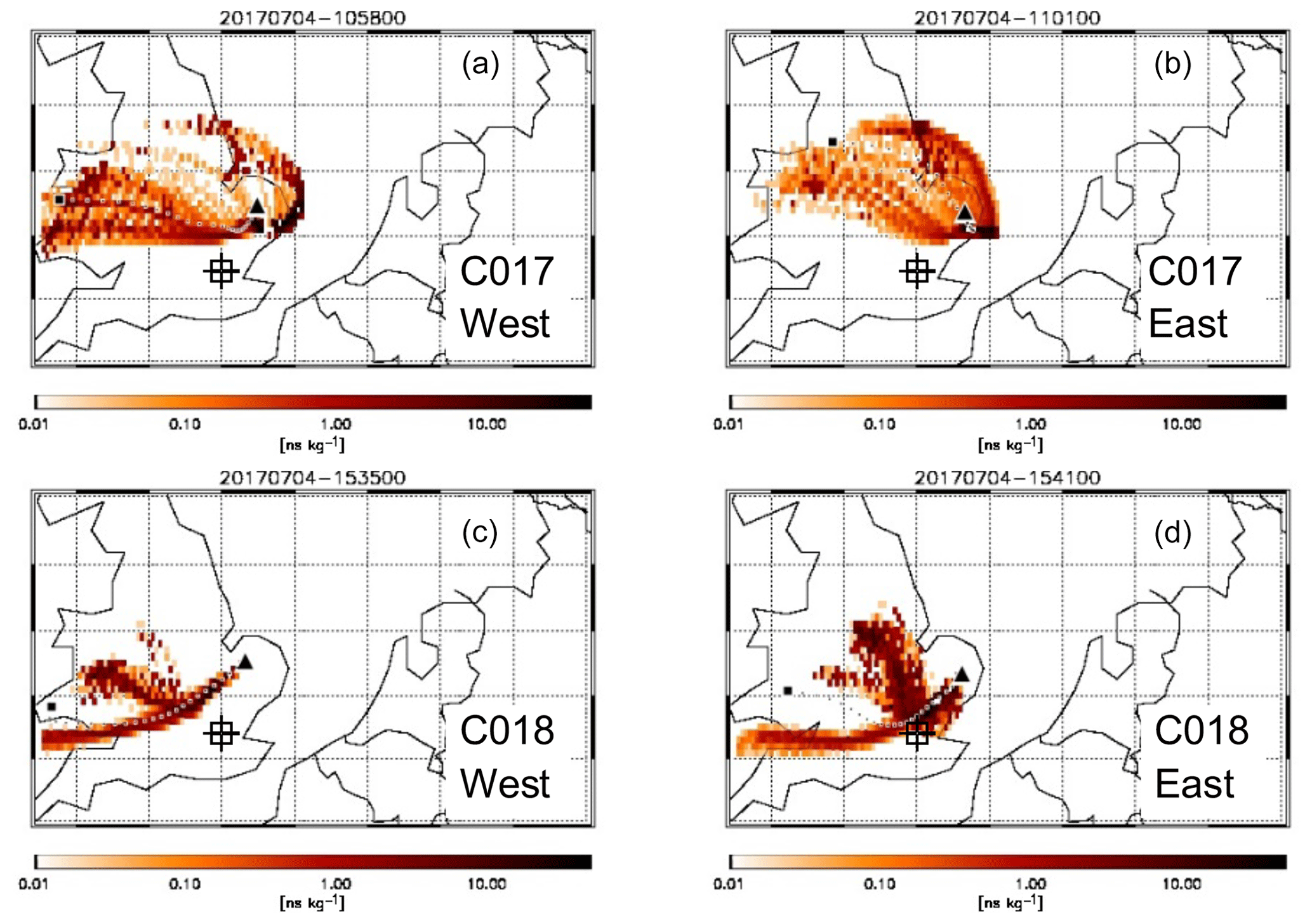
Figure 11 FLEXPART back-trajectories for air masses arriving at the location of FAAM BAe-146 as it intercepted the west (a, c) and east (b, d) plumes during the lowest of the reciprocal runs for flights C017 (a, b) and C018 (c, d). Each coloured pixel indicates the relative contribution of an inert tracer in that air to the total tracer concentration sampled on board. The large black square shows the point of release of the air 24 h prior to interception. The dotted line of black and white squares shows the hourly weighted average trajectory of the air mass based on the relative contributions shown. The square target indicates the approximate position of central London.

A particularly interesting feature of the reciprocal runs for both flights C017 and C018 was the presence of two spatially and chemically distinct elevated areas of pollution, which we refer to as the “west plume” and “east plume”. The west plume was observed in the same location during both morning and afternoon; the east plume was slightly further (∼11 km) to the south and east in the morning, consistent with the back-trajectories (Fig. 11) which show recirculation from the North Sea coast and suggest that, aside from the afternoon east plume, influence from London outflow was minimal in this region. Table 3 provides a summary of the average and peak concentrations for the full leg and the west and east plumes for each reciprocal run and shows that, although not separated far in space or time, the two plumes were chemically distinct at all heights and for both flights. The composition of each plume was consistent across time, although concentrations were generally lower in the morning, suggesting increasing local emissions during the course of the day.

Table 3 Overview of CO, CH₄, NO_x and O₃ and PM (particle number) concentration measured during the reciprocal runs on flights C017 (top) and C018 (bottom). The full flight leg values are averages along each run; the west plume shows the average and maximum (in parentheses) concentrations within the west plume and the same for the east plume. The average altitude is shown for each leg; the average latitude and longitude of the centre of each plume are shown.

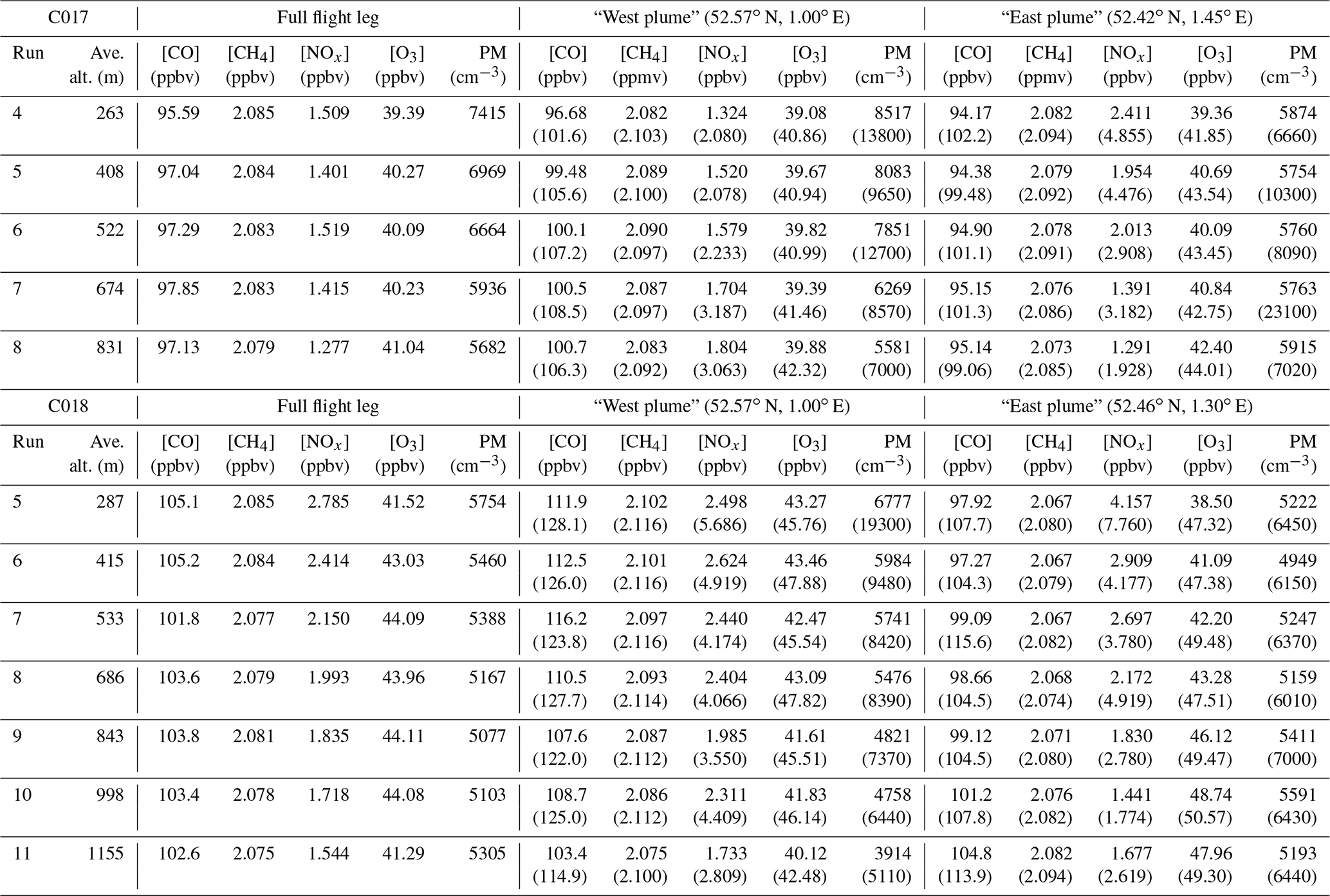
For the whole plume, O₃:NO_x ratios were much lower downwind than upwind for both C017 and C018 (27.3 vs. 40.7 and 21.6 vs. 45.2 ppbv respectively), suggesting that downwind of London we were mostly sampling fresh local emissions. That being said, the highest concentrations of O₃ (up to 48 ppbv) of any of the flights were measured during the downwind legs of C018 in spite of the relatively high NO_x (average mixing ratio of 2.0 ppbv, peaking at ∼5 ppbv).

Total VOC concentrations across the plume during C017 were most strongly correlated with NO_x (r²≈0.97). Further evidence that the pollution sampled in the plume is predominantly derived from local sources comes from the vertical profile of VOCs and particle number concentration. Unlike the London outflow plume sampled on 3 July, the highest concentrations were recorded the following day at the lowest altitude during flight C017 (Fig. 12a). Particle number concentration (particulate matter (PM) in Table 3) was consistently highest at the surface, falling from >7400 at 263 m to 5700 cm⁻³ at 831 m across the full flight leg in the morning and >5700 to 5300 cm⁻³ at 1155 m in the afternoon. This is consistent with fresh emissions of small particles coalescing and coagulating to form a smaller number of larger particles as they are mixed and lofted. By contrast, VOC concentrations along this leg during C018 were strongly correlated with CO and CH₄ (r²≈0.96 and 0.93 respectively) but showed no correlation against either NO_x (r²≈0.07) or particle number concentration (r²≈0.44). The high NO_x levels observed in the plume suggest that local sources are contributing strongly while the high O₃ and correlation of VOCs with long-lived pollutants are indicative of more aged (polluted) air from the south-west. The lowest WAS altitude during C018 was ∼400 m, which makes a direct assessment of the relative contributions of local to transported pollution difficult. In contrast to the morning flight, higher concentrations of VOCs appear to occur at higher altitudes (see Fig. 12b), resulting from a combination of stronger vertical mixing during the afternoon and the influence of long-range transport. Unlike the previous day, however, concentrations increased with altitude to the top of the PBL (at >1 km), suggesting we were sampling well-mixed pollution, rather than a still-distinct fresher London plume as during C016.

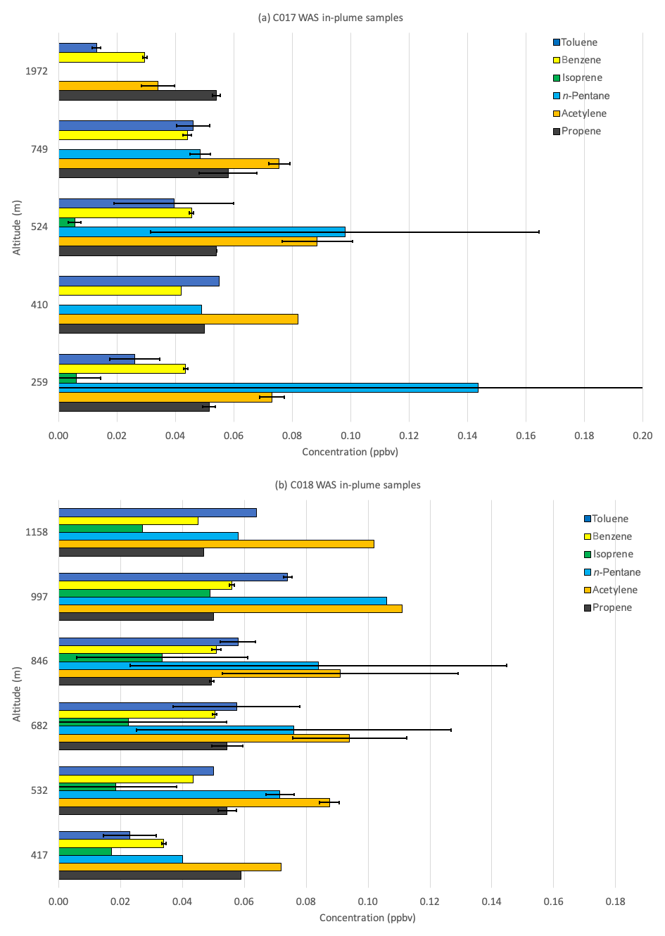
Figure 12 Average concentrations of key VOCs (ppbv) collected via WAS during individual flight legs within the pollution plume detected during (a) flight C017 and (b) flight C018. The average altitude of each flight leg is shown on the y axis. Error bars denote ±1 SD; numbers in square parentheses show the top of error bars.

Absolute and proportional concentrations of isoprene, which is mainly emitted from biogenic sources, were far higher (peaking at 0.05 ppbv vs. <0.01 ppbv) during the afternoon than the morning, as expected given the strong dependence of isoprene emission rates on light and temperature (e.g. Guenther et al., 1991, 1995). During the morning flight, when contributions from local sources were highest, we observed that benzene was well correlated with CH₄ (r²≈0.96) and particle number concentration (r²≈0.92) but less with NO_x (r²≈0.71), whereas toluene showed very weak correlation with any of the continuous measurements. One possible interpretation is that local sources of benzene include a mix of vehicle and industrial (e.g. natural gas processing and petrochemical refining) emissions, while additional toluene emissions originate from non-fossil-fuel-related industries, in particular solvent processing and use, and brewing (e.g. Gibson et al., 1995). Solvent emissions have a large toluene component with no corresponding benzene emissions. Data from the NAEI for VOCs indicate there has been a relative increase over the last decade in the contribution of solvents to toluene emissions, changing the source profile for benzene and toluene. This, taken in conjunction with our findings that local sources can strongly mediate benzene : toluene ratios on small spatial and temporal scales, suggests that their use in identifying the age of urban plumes may be more limited than previously assumed.

For the east plume, only NO_x concentrations were found to be consistently higher in the east plume than the whole leg. Mixing ratios were generally ∼40 % higher in the afternoon than the morning, although the highest NO_x levels (4.85 ppbv) were observed at 263 m in the morning. The maximum increases in NO_x (>200 %) also occurred at the lowest altitude. NO_x concentrations fell rapidly with altitude in the east plume during both flights. NO_x is relatively short-lived and these observations, which were also highly variable in space and time, reflect localised sources rather than long-range transport.

Table 3 also shows evidence of NO_x titration of O₃ in both plumes during the afternoon flight, most pronounced in the east plume and at the lowest altitudes where NO_x levels were highest, with O₃ falling by ∼3 ppbv (∼8 %) due to direct reaction with NO. Outside of the two plumes, O₃ mixing ratios along the entire leg were relatively constant in the morning and afternoon, although slightly higher (∼44 vs. 40 ppbv) during the afternoon flight, as expected for a secondary pollutant formed as a product of the photochemistry. Particle number concentrations were lowest in the east plume. They appeared to fall during the day, with concentrations ∼10 % lower during C018 than C017 consistent with boundary layer effects: the trapping of particles in a stable nocturnal PBL and the dilution effect of the increasing mixed-layer depth over the course of the day. The highest concentrations of CO were observed at higher altitudes than NO_x (∼674 m), which we attribute to long-range transport of polluted air masses from the west and south-west. Average CO concentrations were around 3 ppbv (∼3 %) lower in the east plume than the full leg during both morning and afternoon flights, suggesting that while there were strong local sources of NO_x and VOCs throughout the region, sources of CO and fine particles were largely confined to the west of the run. These observations are consistent with our trajectory analysis (see Fig. 11) that the eastern end of the reciprocal runs receives a flow of (relatively) clean air from the north, resulting in a lower background than the western end.

Concentrations of CH₄ varied little either spatially or temporally across the reciprocal runs or plumes. Although slightly enhanced near the surface, differences were <1 %, suggesting that local sources contribute little to atmospheric CH₄ concentrations in the region.

For the west plume, CO, NO_x and particle number concentrations were all elevated in the west plume relative to the background by as much as 3 ppbv (∼3 %), 1.7 ppbv (>100 %) and 10³ cm⁻³ (15 %) in the morning and ∼15 %, ∼100 % and 20 % in the afternoon. Average CO levels were highest in the west plume during both flights, indicating the strongest sources were located to the western end of the flight track. Vertical distributions were similar with CO concentrations peaking at 108.2 ppbv at 674 m in the morning and 127.7 ppbv at 686 m in the afternoon. The maximum enhancement of CO relative to the entire flight leg was 23 % during C018 at an altitude coinciding with the maximum absolute concentration. We interpret this to indicate CO concentrations in the west plume were dominated by transported air from more industrial areas to the west to north-west of our flights, consistent with our back-trajectory analyses (Fig. 11). NO_x concentrations declined more slowly with altitude in the west than the east plume during the morning. In the afternoon, aside from an enhancement observed during the lowest flight leg, NO_x peaked at 998 m, which is also where the maximum elevation relative to the entire reciprocal run occurred. The NO_x-to-CO ratio is relatively low in the west plume, suggesting that there was a greater proportion of more aged air at this end of the run, although the surface elevation shows there are also strong local sources of NO_x.

Particle number concentration was much higher in the west than the east plume during both flights but was also much higher (∼25 %) in the afternoon than morning. The largest increase in number in the west plume occurred near the surface (altitudes up to 522 m) in the morning and at 283 m in the afternoon, indicating substantial local sources of PM. AMS data, only available for the afternoon flight (C018), further support the apparent difference in emission source and strength between the eastern and western ends of the reciprocal runs, with the west plume showing an increase in fine particulate matter (PM1) indicative of fresh emissions. The increase was mostly due to high levels of organic and nitrate aerosols.

For the attribution, by combining our back-trajectories for air masses sampled in each plume with UK NAEI data for the region, we were able to identify local point sources to which the observed east and west plumes are likely to be attributable. For CO, NO_x and PM1 we calculated a “source intensity” at the point of interception, based on an assumption that concentrations decayed with the inverse square of distance from the source (i.e. neglecting wind dispersion and chemical transformation).

The largest local contributions to CO in the west plume were power stations at Thetford and Ely in the morning, but the slight change in wind direction in the afternoon resulted in large additional contributions from local construction and food and drink manufacturers. The same point sources also made the biggest contribution to NO_x in the west plume. Landfill gas combustion and brick manufacturing were likely the principal local sources of PM1 throughout the day in both plumes. Power stations again contributed strongly to the west plume and probably account for the high nitrate component of the fine particles observed in this plume, while landfill gas combustion and emissions from British Sugar are high in organic matter.

The only major local source of CO to the east plume was a British Sugar processing facility, and that was only directly upwind during the afternoon. There were fewer (and weaker) sources of PM at the eastern end of the reciprocal run, resulting in the low particle number concentrations observed. There was no obvious point source of NO_x in the eastern end of the reciprocal runs, and we speculate the very high levels observed in the east plume are the result of traffic emissions, particularly from the junctions between the major A144, A146 and A143 roads which were almost directly flown over.

4 Conclusions

We report here measurements of atmospheric conditions and composition made from the UK's FAAM BAe-146-301 Atmospheric Research Aircraft during three research flights over a 2 d period in July 2017. Conditions were favourable for all flights, and a change in wind speed and direction overnight enabled us to sample contrasting pollution events.

On 3 July, moderate west-south-westerly winds produced a narrow distinct plume of pollution outflowing London. The clear edges and strong enhancement of the plume allowed us to estimate emissions of long-lived pollutants from the urban area. Our calculated fluxes of CO₂ agreed well with those previously reported for 2012 by O'Shea et al. (2014), but our estimated emissions of CO were a factor of 2 lower and CH₄ was a factor of 2 higher. These differences between campaigns are likely due to differences in emissions sources and strengths within the flux footprint and the inherent sensitivity of the method to the surface sampled and the methodology applied. Methods such as those employed in Pitt et al. (2019) that can provide improved quantification of surface interaction are of greater use when the emission source is not distinct from its surroundings.

The second and third flights on 4 July experienced much lighter and more variable winds with the result that pollution was more widely dispersed and derived from a mixture of sources. In general, there was evidence of a strong contribution of fresh emissions from local point sources mixing with air transported from further afield bringing more aged pollution to the region. We observed clear pollution events over northern East Anglia during both flights and flew a series of reciprocal runs to sample these peaks over the full altitude of the boundary layer. Continuous real-time measurements of long-lived gas-phase and aerosol pollutants were supplemented with analysis of a range of volatile organic compounds from whole-air samples taken during the reciprocal runs.

WAS has previously been successfully deployed on the ground and from aircraft to complement real-time measurements and to identify sources (e.g. Tiwari et al., 2010; Breton et al., 2017; Aruffo et al., 2014; Warneke et al., 2013; Cain et al., 2017; Lee et al., 2018). Tiwari et al. (2010) reported high concentrations of ethane, propane and n-butane in Yokohama, Japan, which they attributed to fugitive emissions from petroleum refining and evaporation. Ethane, propane, n-butane and cyclopentane made up the highest proportion of VOCs across all three flights. While there are a considerable number of petrochemical refining and natural gas processing facilities around London, the presence of these VOCs was too ubiquitous for us to be able to unambiguously determine the source.

Based on different relative abundances of VOCs and the ratio of O₃:NO_x we were able to determine source sectors and individual sources for the pollution events on 4 July. During the morning most of the transported air mass was from the north and west, and therefore relatively clean, and the pollution was predominantly fresh emissions from local food and drink and construction industries. By contrast, the air mass in the afternoon contained more aged pollution from the south-west, although still very little from the London area. We were able to attribute local emissions to the same sources combined with a contribution from power plants in the area. The high NO_x concentrations observed toward the eastern end of the reciprocal runs appeared to emanate from traffic at a series of major road junctions.

Importantly though, our observations of local pollution episodes on 4 July strongly suggest that the use of the ratio of benzene to toluene concentrations to assess air mass age and emission source is unreliable when applied over small spatial and temporal scales. The increasing numbers of sources that emit toluene alone result in heterogeneous ratios of benzene to toluene emissions from different source sectors, whereas the use of concentration ratios is based on assumed constant relative source intensities.

These three flights give a clear demonstration of the power of airborne measurements which can be used for targeted campaigns to provide direct source attribution (or test hypotheses of sources) and for longitudinal studies over time to provide evidence of new or changing emission sources or source profiles, and to inform and constrain bottom-up emissions inventories. They also provide clear evidence that even in a region where background pollution concentrations are dominated by emissions from a megacity, relatively small point sources can still play a significant role in local air pollution, particularly downwind where they exacerbate already high levels. The factors that control the build-up of air pollution in the London area are various and multiple: local emissions, transport from distant sources, and terrestrial and marine emissions. In the highly complex environment around a megacity, where a high background level of pollution mixes with a variety of local sources at a range of spatial and temporal scales, the use of unvarying VOC : VOC ratios may not be valid given the different ages of the air. It is necessary to consider and constrain all of the contributing factors to understand the problem and to develop effective mitigation and control strategies.