Sesquiterpenes dominate monoterpenes in northern wetland emissions

We have studied biogenic volatile organic compound (BVOC) emissions and their ambient concentrations at a sub-Arctic wetland (Lompolojänkkä, Finland), which is an open, nutrient-rich sedge fen and a part of the Pallas-Sodankylä Global Atmosphere Watch (GAW) station. Measurements were conducted during the growing season in 2018 using an in situ thermal-desorption–gas-chromatograph–mass-spectrometer (TD-GC-MS).

Earlier studies have shown that isoprene is emitted from boreal wetlands, and it also turned out to be the most abundant compound in the current study. Monoterpene (MT) emissions were generally less than 10 % of the isoprene emissions (mean isoprene emission over the growing season, 44 µg m⁻² h⁻¹), but sesquiterpene (SQT) emissions were higher than MT emissions all the time. The main MTs emitted were α-pinene, 1,8-cineol, myrcene, limonene and 3Δ-carene. Of SQTs cadinene, β-cadinene and α-farnesene had the major contribution. During early growing season the SQT∕MT emission rate ratio was ∼10, but it became smaller as summer proceeded, being only ∼3 in July. Isoprene, MT and SQT emissions were exponentially dependent on temperature (correlation coefficients (R²) 0.75, 0.66 and 0.52, respectively). Isoprene emission rates were also found to be exponentially correlated with the gross primary production of CO₂ (R²=0.85 in July).

Even with the higher emissions from the wetland, ambient air concentrations of isoprene were on average > 100, > 10 and > 6 times lower than MT concentrations in May, June and July, respectively. This indicates that wetland was not the only source affecting atmospheric concentrations at the site, but surrounding coniferous forests, which are high MT emitters, contribute as well. Daily mean MT concentrations had high negative exponential correlation (R²=0.96) with daily mean ozone concentrations indicating that vegetation emissions can be a significant chemical sink of ozone in this sub-Arctic area.

1 Introduction

Many plants communicate by releasing massive amounts of biogenic volatile organic compounds (BVOCs) into the air. They can either attract pollinators, repel herbivores or respond to other stress. Globally, these biogenic emissions are estimated to reach 760 Tg C yr⁻¹ and chemically consist mainly of isoprene (C₅H₈), monoterpenes (MTs, C₁₀H₁₆), sesquiterpenes (SQTs, C₁₅H₂₄), methanol and acetone (Sindelarova et al., 2014). The terrestrial BVOCs account for about 90 % of the emission total (Guenther et al., 1995).

The global climate change has been estimated to produce the greatest warming in the high northern latitudes (IPCC, 2018). Many plant species in these ecosystems are at the northernmost limits of their existence and even small changes in, for example, temperature and hydrology may severely influence vegetation composition and thus biosphere–atmosphere interactions and trace gas fluxes. The warming is likely to increase the emissions of BVOCs into the atmosphere. Most of these emitted compounds have high reactivity in the atmosphere and their lifetimes vary from minutes to hours. These volatile organic compounds (VOCs) are oxidised mainly by the hydroxyl radicals, ozone and nitrate radicals, and their oxidation products affect the secondary organic aerosol (SOA) formation, ozone fluxes and oxidative capacity of the air, therefore having strong effects on air quality and climate. Knowing the current biogenic emissions in a very pristine sub-Arctic environment will be valuable later when assessing the impact of progressing climate change in the Arctic region.

Knowledge of the biogenic emissions in the sub-Arctic/Arctic area is very limited, at least partly because emissions are assumed to be low there due to low temperatures, short summers and low vegetation biomass. However, atmospheric reactions such as SOA and ozone formation/destruction are regional rather than global processes (Tunved et al., 2006). Therefore these relatively low emissions can have high impacts in this very pristine environment. In addition, Kramshoj et al. (2016) showed that temperature dependence of BVOC emissions in the Arctic can be significantly higher than in tropical ecosystems. Therefore, the predicted temperature change has a vast influence on the BVOC emissions and will cause a significant rise compared to the observations so far.

Wetlands cover an area of about 2 % of the total land surface area of the world. Most of the wetlands are located in the boreal and tundra zones on the Northern Hemisphere (Archibold, 1995). Approximately 3.5×10⁶ km² of boreal and sub-Arctic peatlands exist in Russia, Canada, the United States (Alaska) and Fennoscandia (Finland and the Scandinavian countries).

Northern wetlands are important sinks for carbon dioxide and sources of methane, but knowledge on their VOC emissions is very limited. Studies have shown, that northern wetlands are high isoprene emitters (Janson and Serves, 1998; Haapanala et al., 2006; Hellén et al., 2006; Ekberg et al., 2009; Holst et al., 2010), but very little is known about the physiological and environmental regulations of isoprene fluxes especially in colder sub-Arctic environments and even less is known on the emissions of other VOCs. These other VOCs (e.g. mono- and sesquiterpenes) may have stronger effects on SOA formation even with lower emissions due to their higher SOA formation potentials compared to isoprene (Lee et al., 2006).

We have studied VOC emissions and their ambient concentrations at a Finnish sub-Arctic wetland (Lompolojänkkä), which is an open, nutrient-rich sedge fen (Lohila et al., 2015) and a part of the Pallas-Sodankylä Global Atmosphere Watch (GAW) station.

2 Experimental set-up

2.1 Measurement site

The measurements were conducted in 2018 in a northern boreal fen, Lompolojänkkä, in the Pallas-Yllästunturi National Park, Finland. The Lompolojänkkä measurement site is an open, nutrient-rich sedge fen located in the aapa mire region of north-western Finland (67^∘59.832^′ N, 24^∘12.551^′ E, 269 m a.s.l.; Aurela et al., 2009, 2015; Lohila et al., 2010, 2015). The relatively dense vegetation layer is dominated by dwarf birches (Betula nana), bogbeans (Menyanthes trifoliate), downy willows (Salix lapponum) and sedges (Carex spp.). The mean vegetation height on the fen is 40 cm. The moss cover on the ground is patchy (57 % coverage), consisting mainly of peat mosses (Sphagnum angustifolium, S. riparium and S. fallax) and some brown mosses (Warnstorfia exannulata). This aapa mire is characterised by a relatively high water level, with almost the entire peat profile being water-saturated throughout the year. The maximum peat thickness is 3 m. The site is surrounded by coniferous forest, which consists mainly of Scots pine (Pinus sylvestris) (72 % of the forest area) with some Norway spruce (Picea abies) (20 %) and deciduous trees (mainly Betula pubescens, some Populus tremula and Salix spp.) (8 %) (Lohila et al., 2015).

2.2 Emission measurements

The measurement set-up consisted of a $\mathrm{60}\times \mathrm{60}\times \mathrm{25}$ cm fluorinated ethylene propylene (FEP) chamber, which was flushed with 4 L min⁻¹ of volatile organic compound (VOC) free air generated by a commercial catalytic converter (HPZA-7000, Parker Hannifin Corporation). Due to high reactivity of the studied compounds, their ambient air concentrations at this remote location are much lower than concentrations in our emission chamber. Mean concentrations in the chamber were 10 400, 2300 and 57 000 ng m⁻³ for SQTs, MTs and isoprene, respectively. Therefore we do not expect to create any artificial emission by using zero air. The thermal-desorption–gas-chromatograph–mass-spectrometer (TD-GC-MS) was connected to the chamber via a 21 m long, 4 mm (i.d.) tubing heated a few degrees above the ambient temperature and pumped with 0.5 L min⁻¹ make-up flow, followed by a 2.5 m long, 1 mm (i.d.) tube, with a flow of 40 mL min⁻¹. All tubing was made of FEP. For in situ analysis the VOC samples were collected directly into a standard low-flow cold trap filled with Tenax TA (50 %) and Carbopack B (50 %) of the TD-GC-MS for 30 min every 2 h in May–June and every hour in July. The trap was kept at 20 ^∘C during sampling to prevent water vapour present in the air from accumulating in the trap. Offline samples were taken at the end of July using Tenax TA/Carbopack B adsorbent tubes. Sampling flow was ∼55 mL min⁻¹. Sampling time for tubes was 2 h during the day and 10 h during the night. Breakthrough of isoprene was possible during 10 h sampling. However, there were only three 10 h samples taken, and they were overnight, when the emissions were very low. Samples were analysed later in the laboratory of the Finnish Meteorological Institute.

Two custom-built data loggers were used during the campaign. From April to mid-July the set-up consisted of a thermistor (Philips KTY 80/110, Royal Philips Electronics, Amsterdam, Netherlands) for the temperature inside the chamber and a quantum sensor (LI-190SZ, LI-COR, Biosciences, Lincoln, USA) for the photosynthetically active radiation (PAR), measured just above the enclosure. In mid-July this data logger had technical problems, so a replacement was used. The new data logger used an LM35 (Texas Instruments, Dallas, USA) temperature sensor and an SQ-520 (Apogee Instruments Inc., Logan, USA) quantum sensor for PAR.

The temperature inside the soil chamber sometimes increased to > 40 ^∘C (9 out of 264 measurement points). This is clearly higher than ambient air temperature, which stayed below 29 ^∘C all the time. Due to this heat stress some additional emissions may have been induced. However, low vegetation canopies in high-latitude ecosystems have been observed to have canopy temperatures up to 15 ^∘C warmer than the ambient air temperature during clear-sky conditions (Rinnan et al., 2014). Highest differences between the air temperature measured at the height of 3 m and soil chamber temperature were observed during the hot summer days with clear-sky conditions. A difference > 15 ^∘C was observed for 24 samples out of 264 samples. The mean difference was 4.6 ^∘C. Due to this heat stress, emission rates shown are expected to be overestimated during clear-sky conditions, but this is not expected to affect emission potentials, which are normalised to 30 ^∘C. Sometimes heating can cause additional stress, for example due to drought, but at this very moist wetland this was not a problem.

Figure 1 Vegetation cover of the measured frames at the beginning of July in 2018.

Three different stainless steel frames located close to the measurement cabin in the middle of the fen were used for the emission measurements. Stainless steel frames were installed into the fen 8 months before starting the measurements. Vegetation at frame 1 was dominated by forbs (Menyanthes trifoliate, Comarum palustre, Equisetum fluviatile) and different sedges and sphagnum moss species (Fig. 1). Vegetation in frame 2 consisted of two willow species (Salix lapponum, Salix phylicifolia), purple marshlocks (Comarum palustre), and various sedge and sphagnum moss species. Vegetation in frame 3 was dominated by different sedges and sphagnum moss species together with smaller amount of dwarf birch (Betula nana), downy willows (Salix lapponum), purple marshlocks (Comarum palustre) and horsetails (Equisetum fluviatile).

2.3 Ambient air measurements

Ambient air samples were collected through a 21 m long FEP tubing (o.d. 1∕4 in., i.d. 1∕8 in.), which was heated to 5 ^∘C higher than ambient temperature. The flow through the tube was 0.5 L min⁻¹. A stainless steel (grade 304) inlet line of 1 m was heated to 120 ^∘C in order to destroy O₃. This O₃ removal method is described in detail by Hellén et al. (2012). Removal of O₃ from the inlet flow before collection of the sample is essential for avoiding losses of the very O₃-reactive compounds (e.g. β-caryophyllene). VOCs in a 40 mL min⁻¹ subsample were collected from the main inlet flow for 30 min every other hour directly in the cold trap of the thermal-desorption unit. Samples were taken at the height of 1.5 m in the middle of the fen. In total, 273 ambient air samples were analysed in May–July 2018.

2.4 GC-MS analysis

The in situ TD-GC-MS consisted of a thermal desorption unit (Turbo Matrix 650) followed by a gas chromatograph (Clarus 680) and a mass spectrometer (Clarus SQ8 T), all manufactured by Perkin-Elmer. An HP-5 column (60 m; i.d. 0.25 mm; film thickness 1 µm; Agilent Technologies, Santa Clara, California, US) was used for the separation. The column was first heated from 50 to 150 ^∘C at the rate of 4 ^∘C min⁻¹ and then at the rate of 8 ^∘C min⁻¹ up to 250 ^∘C, where it was kept for 5 min. The total time of the analysis was 42.50 min.

The instrument was located in a cabin in the middle of the fen. A five-point calibration was performed using liquid standards in methanol solutions. Standard solutions (5 µL) were injected onto adsorbent tubes and then flushed with nitrogen (80–100 mL min⁻¹) for 10 min to remove the methanol. All the studied MTs (α-pinene, camphene, β-pinene, 3Δ-carene, p-cymene, 1,8-cineol, limonene, myrcene, terpinolene and linalool) and following SQTs were included in the calibration solutions: longicyclene, iso-longifolene, α-gurgunene, β-caryophyllene, β-farnesene and α-humulene. Unknown sesquiterpenes were tentatively identified based on the comparison of the mass spectra and retention indexes (RIs) with NIST mass spectral library (NIST/EPA/NIH Mass Spectral Library, version 2.0). RIs were calculated for all SQTs using RIs of known SQTs and MTs as reference. These tentatively identified SQTs were quantified using response factors of calibrated SQTs having the closest mass spectra resemblance. Isoprene was calibrated using a gaseous standard (National Physical Laboratory, 32 VOC mix at 4  ppb level).

Offline samples taken on adsorbent tubes at the end of July were analysed using the same method as for the in situ samples. TD-GC-MS used for the adsorbent tubes consisted of an automatic TD unit (TurboMatrix 650) connected to a GC (Clarus 600) coupled to a quadrupole MS (Clarus 600 T), all purchased from PerkinElmer Inc. (Waltham, MA, USA).

Detection limits for emission measurements were 0.002–0.055 µg m⁻² h⁻¹ and 0.3–5.1 pptv for ambient air measurements (see Supplement Table S2). For calibrated compounds analytical precision calculated as a standard deviation of the calibration standards (N=6) varied between 1.5 % and 5 %, and uncertainty estimated by following ACTRIS (Aerosol Clouds Trace gases Research InfraStructure) guidelines (ACTRIS, 2018) was between 17 and 25 %. Recoveries of the studied compounds from the inlet (relative humidity 0 % and 100 %) and soil chamber (relative humidity 0 %) used were > 80 %. However, linalool, bornylacetate and β-farnesene suffered from losses in the online mode of the TD system at low humidity. In the soil emission samples humidity was high all the time and in the ambient air linalool, bornylacetate and β-farnesene concentrations were minor. The method validation has been described in detail by Helin et al. (2020).

2.5 Complementary data

The net ecosystem CO₂ exchange (NEE) between the biosphere and the atmosphere was measured by the eddy covariance method. The instrumentation consisted of a USA-1 (METEK) sonic anemometer and a closed-path LI-7000 (LI-COR, Inc.) CO₂∕H₂O gas analyser with a measurement height of 3 m (Aurela et al., 2009). Gross primary production (GPP) was determined from the NEE data utilising standard partitioning procedures by estimating the respiration (R) from night-time NEE data and calculating GPP as the remainder of NEE and R (GPP = NEE-R) (e.g. Reichstein et al., 2005).

Supporting meteorological measurements, including air temperature (Vaisala, humidity and temperature probe, HMP), soil temperatures (temperature sensor, PT100) at various levels, water table level (WTL) (PDCR1830) and PAR (LI-COR, LI-190SZ), were collected by a Vaisala QLI-50 data logger as 30 min averages.

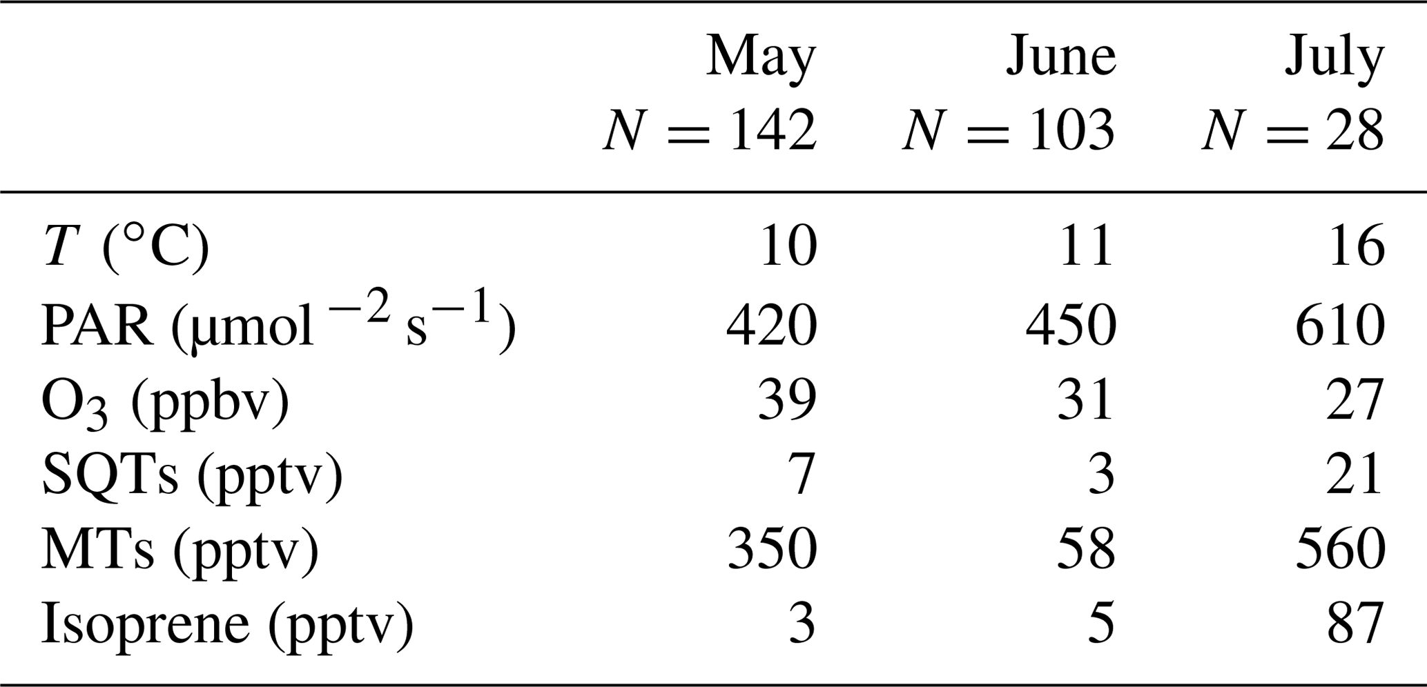
Table 1 Mean chamber temperature (T), photosynthetically active radiation (PAR), temperature and light activity coefficient (CT × CL, Guenther et al., 1993) and emission rates (E) of monoterpenes (MTs), sesquiterpenes (SQTs) and isoprene during the various sampling periods. F1(a): frame 1; F2: frame 2; F1(b): frame 1; F3: frame 3; F1(T): tube samples from frame 1. (< DL: below detection limit).

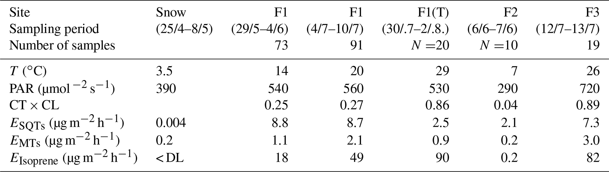
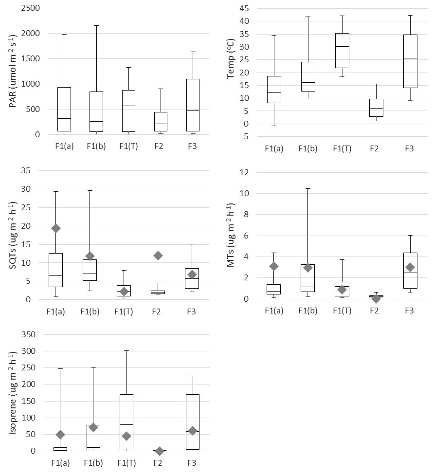
Figure 2 Mean box-and-whisker plots of photosynthetically active radiation (PAR), temperature (Temp), and emission rates of sesquiterpenes (SQTs), monoterpenes (MTs) and isoprene during the various emission measurement periods. The boxes represent first and third quartiles and the horizontal lines in the boxes the median values. The whiskers show the highest and lowest observations. Grey diamonds represent monthly mean emission potentials (T=30 ^∘C) and diamonds emission potential (T=30 ^∘C and PAR =1000 µmol ⁻² s⁻¹). F1(a): frame 1 in 29 May–4 June; F2: frame 2 in 6–7 June; F1(b): frame 1 in 4–10 July; F3: frame 12–13 July; F1(T): tube samples from frame 1 in 30 July–2 August.

3 Results and discussion

3.1 Terpenoid emissions and their environmental drivers

Earlier studies have shown that isoprene is emitted from wetlands (Jansson and de Serves, 1998; Haapanala et al., 2006; Hellén et al., 2006), and it also turned out to be the most abundant compound in the current study (Table 1 and Fig. 2). Isoprene emissions are dependent on temperature and light, and therefore they are also connected to CO₂ GPP as shown in Fig. 3. During the first 2 d in June, solar radiation was very high and temperature in the enclosure also increased, which is shown by the high light and temperature activity coefficients in Fig. 3. This caused unexpectedly high isoprene emissions that clearly deviated from the general curve. The light and temperature activity coefficient (CT × CL) is described by Guenther et al. (1993) and are shown in Table 1 for each of the measurement periods separately.

MT emissions were generally less than 10 % of the isoprene emissions, but SQT emissions were surprisingly high and exceeded MT emissions all the time (Table 1 and Fig. 2). To our knowledge, this is the first time SQT emissions have been measured from wetlands, although Faubert et al. (2010, 2011) detected emissions of SQTs from boreal peatland samples in laboratory experiments. Usually in the emissions from the vegetation, MTs are several times higher than SQTs (e.g. Messina et al., 2016), but here in the wetland emissions it was the opposite. During the early growing season, SQT emission rates were about 10 times higher than MT emission rates, but this difference became smaller since MT emissions increased as summer proceeded and reached their maximum in July, while SQT emission rates remained at about the same level until August. Late-summer SQT emission rates were still about twice as high as MT. These high early-summer SQT emissions could be due to compounds produced in the soil and trapped in frozen soil and snow cover during winter. Aaltonen et al. (2012) measured VOCs in the snow cover in boreal forest in southern Finland and found both MTs and SQTs in snow with a decreasing trend from the soil surface to the top layer of snow, indicating soil as a source for terpenoids. These compounds can then be released to the air when the snow and ground melt.

Table 2 The most abundant MTs and SQTs in the emissions at Lompolojänkkä fen during each measurement period. F1–3 indicates the measured frame.

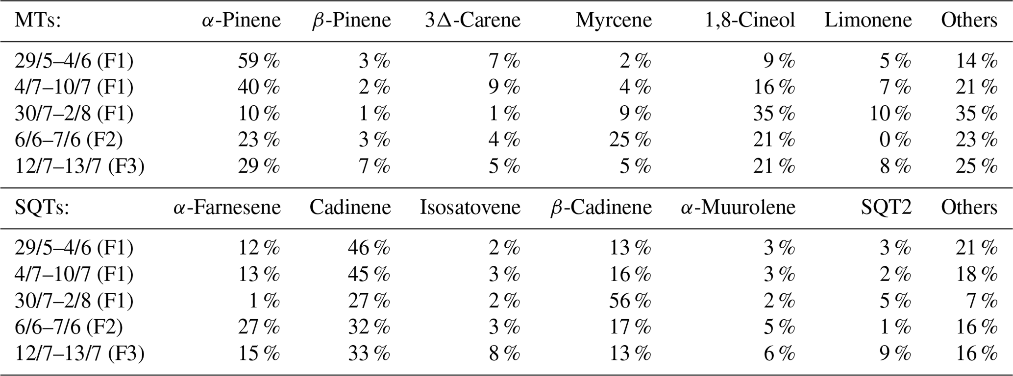
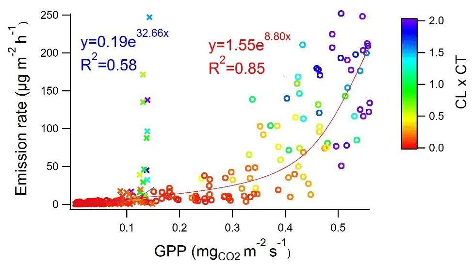
Figure 3 Isoprene emission rate vs. CO₂ gross primary production (GPP) at the beginning of summer (29 May–7 June; crosses and red fitting) and in July (4–13 July; dots and blue fitting) measured at Lompolojänkkä fen in summer 2018. Colour corresponds to the strength of the light and temperature activation coefficient (CL × CT) in the range of 0.0–2.0. R² values are from the corresponding transformed straight lines (ln(y), ln(x)).

The emission patterns of both MTs and SQTs varied during the measurements. In Table 2, we show the six most abundant compounds, both for SQTs and MTs. The most abundant MT was α-pinene at the beginning of measurements, and it remained the most copious one until August, when 1,8-cineol exceeded α-pinene emissions. The most abundant SQT was cadinene replaced by β-cadinene in August (cadinenes are tentative identifications). Altogether, we identified 19 SQTs (Table S1), but we had standards for only 8 of them. The rest are identified and quantified as described in Sect. 2.4.

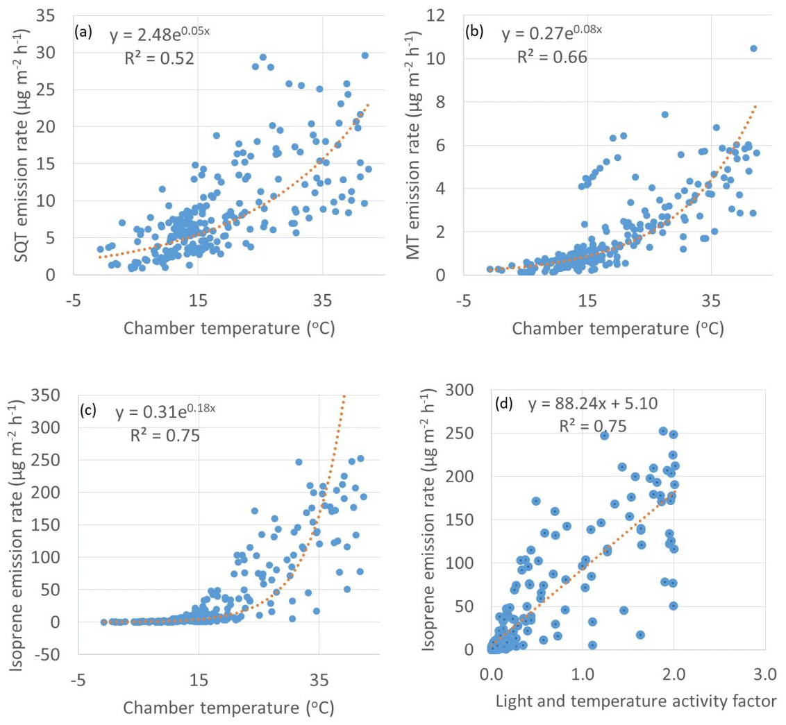
Figure 4 Exponential correlations of temperature with emission rates of (a) SQTs, (b) MTs and (c) isoprene and (d) linear correlation of light and activity coefficient (Guenther et al., 1993) with emission rates of isoprene. R² values for the plots (a)–(c) are from the corresponding transformed straight lines (ln(y), ln(x)).

Both MT and SQT emissions were dependent on temperature as shown in Fig. 4. The β-coefficient (as described by Guenther et al., 1993) for MTs was 0.08 which is close to 0.09 often observed for terrestrial plants. The coefficient was lower for SQT (0.05). Lower coefficients have been previously observed also for SQT emissions from a Norway spruce (Hakola et al., 2017). For individual MTs and SQTs the β-coefficient varied between 0.05 and 0.14 and between 0.04 and 0.10, respectively (Table S3). The β-coefficient of isoprene was 0.18. A temperature sensitivity of isoprene higher than this has been observed at a dry Arctic heath by Kramshoj et al. (2016). In their studies, warming of 3.1 ^∘C caused a 240 % increase in isoprene emissions. They speculate that the large response to warming may be linked to the effects of decreased soil moisture, which may limit the natural cooling evapotranspiration process, resulting in higher leaf temperatures at this dry Arctic site.

SQT emissions were better correlated with soil temperature than chamber temperature in early summer, when soil temperature was below 15 ^∘C (Fig. 5) and vegetation was sparse (Fig. 6). This is additional proof of the hypothesis that SQTs are produced under the snow due to microbiological activity and released when snow is melting and the soil thawing. Later on, new growth affects the emissions, correlation with soil temperature weakens, and correlation with chamber temperature increases. For MTs and especially for isoprene, chamber temperature also had better correlation in early summer indicating a stronger effect of new growth also then.

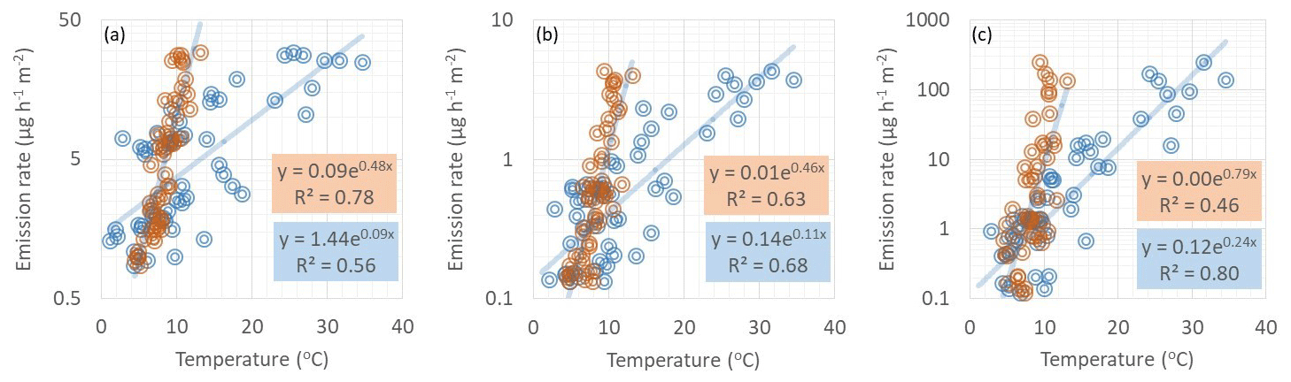
Figure 5 Correlation of (a) SQTs, (b) MTs and (c) isoprene emission rates with soil (orange dots) and chamber (blue dots) temperatures during the early growing season on 1–7 June 2018. Soil temperature was measured 5 cm below the soil surface close to our emission chamber. R² values are from the corresponding transformed straight lines (ln(y), ln(x)).

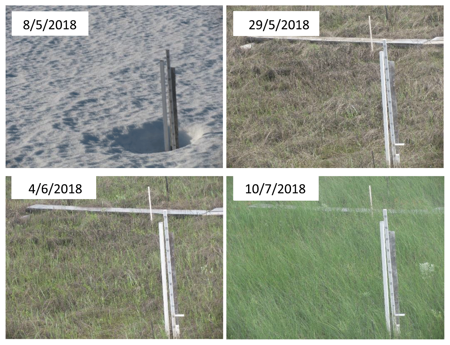
Figure 6 Variation in the vegetation cover at Lompolojänkkä fen over the growing season in 2018.

The mean diurnal variation in emissions of all terpenes followed the variations in temperature and PAR (Fig. 7). The isoprene emission is light dependent and the emissions were not detected during the night, but MTs and SQTs were also emitted then. During the night-time SQTs were clearly the most significant compound group, emitted both in early and mid-summer. Also, diel curves clearly show that SQT emissions were unexpectedly high in early summer (Fig. 7), which was also shown as high emission rates (Table 1). The Supplement Fig. S1 shows the mean diurnal variation in the individual SQTs and MTs for the same periods. The relative contribution of an SQT, β-cadinene, clearly increases during the daytime. For the MTs, a daytime increase was observed for the 1,8-cineol, myrcene and limonene. Higher daytime contribution could indicate a light-dependent source of these compounds. Earlier light dependence of 1,8-cineol emissions has been observed in Scots pine emissions (Tarvainen et al., 2005).

Mean emission potentials (at 30 ^∘C) of SQTs (Fig. 2) decreased over the growing season, while the emission potentials of MTs stayed at the same level and isoprene potentials slightly increased, indicating different source mechanisms for these compounds.

Figure 7 Diurnal variation in chamber temperature, PAR and emission rates (µg m⁻² h⁻¹) of isoprene, SQTs and MTs.

Figure 8 An estimate of the potential importance of emissions of different BVOC groups for SOA production. For calculating the SOA flux, BVOC emissions were weighted by the mean SOA yields found by Lee et al. (2006) in photo-oxidation chamber studies (SQT 68 %, MT 32 % and isoprene 2 %). F1(a): frame 1 in 29 May–4 June; F2: frame 2 in 6–7 June; F1(b): frame 1 in 4–10 July; F3: frame 12–13 July; F1(T): tube samples from frame 1 in 30 July–2 August.

There is very little information available on the emissions of individual plant species growing at the Lompolojänkkä fen. Salix species generally have high isoprene emissions (Iseprands et al., 1999; Kramshoj et al., 2016), and wetland sedges are also known to be strong isoprene emitters (Ekberg et al., 2009). Sphagnum moss is low emitter of both isoprene and MTs (Tiiva et al., 2009; Iseprands et al., 1999; Faubert et al., 2010). However, there is knowledge available on the emissions of wetlands especially for the isoprene. The mean emission potential of isoprene (93 µg h⁻¹ m⁻² at 30 ^∘C and 1000 µmol ⁻² s⁻¹) at the Lompolojänkkä fen was lower than that measured earlier at a boreal fen in southern Finland. In a study by Haapanala et al. (2009) the emission potential measured with ecosystem-scale flux measurements using a relaxed eddy accumulation technique in the southern boreal fen was on average 680 µg h⁻¹ m⁻², while the emission potential measured using chambers was only 224 µg h⁻¹ m⁻² (Hellén et al., 2006). A reason for the high difference could be cold and rainy weather during the chamber measurements. If emissions rates with low (< 0.2) light and temperature activation values (CT × CL) were used from ecosystem-scale fluxes, the emission potential was only 330 µg h⁻¹ m⁻². There have also been great differences in other earlier wetland studies. Janson and De Serves (1998) found high isoprene emission potentials (620 µg h⁻¹ m⁻²) at wet southern boreal fen sites (flarks), while a clearly lower potential (17 µg h⁻¹ m⁻²) was measured for a dry site (hummock). In addition, Holst et al. (2010) measured ecosystem-scale fluxes with a proton transfer reaction mass spectrometer (PTR-MS) at a sub-Arctic wetland in northern Sweden and found a very high emission potential (1150 µg h⁻¹ m⁻²) for isoprene.

Using a gradient method to measure BVOC fluxes above a boreal mixed forest very close to the Lompolojänkkä site, Rinne et al. (2000) observed a mean MT emission potential (at 30 ^∘C) of 860 µg m⁻² h⁻¹, which is clearly higher than the mean emission potential of MTs (3 µg m⁻² h⁻¹) found for the Lompolojänkkä fen in our study. SQTs were not measured by Rinne et al. (2000), but in our study the mean emission potential of SQTs from Lompolojänkkä (11 µg m⁻² h⁻¹) was only ∼1.5 % of the emission potential of MTs found for the forest by Rinne et al. (2000). Mean isoprene fluxes (14.4 µg m⁻² h⁻¹) measured by Rinne et al. (2000) above this northern boreal forest were ∼10 times lower than MT fluxes while in our study isoprene emission potential from the Lompolojänkkä fen was clearly higher (93 µg m⁻² h⁻¹) than for MTs. In an earlier study on a sub-Arctic wetland in Sweden, a much higher emission potential (1150 µg h⁻¹ m⁻²) for isoprene has even been observed (Holst et al., 2010). Since the wetlands cover large areas in the sub-Arctic, they can be a significant source of isoprene, in particular, even compared to the emissions of the forests.

SQTs are very reactive and have higher SOA yields than MTs or isoprene (e.g. Lee et al., 2006), and therefore even lower emissions can have strong impacts on local chemistry and on aerosol formation and growth. To get a rough estimate of the importance of different compound groups for SOA production, emission rates were weighted by the SOA yields found from the literature. Yields were obtained from a photo-oxidation chamber study by Lee et al. (2006), where the same set-up was used for studying the SOA production of isoprene, MTs and SQTs. Yields for isoprene, α-pinene (MT) and β-caryophyllene (SQT) were 2 %, 32 % and 68 %, respectively. In a real environment there are lots of factors (e.g. meteorology, pre-existing aerosol load, oxidant, individual MTs and SQTs, and NO_x concentrations) affecting the SOA production, and therefore this just gives a rough estimate. However, results indicate that SQTs are the main SOA source at this wetland site, especially during the early growing season (Fig. 8). SQTs emitted by the forests are often already oxidised inside the canopy (Zhou et al., 2017), and oxidation products may be lost on canopy surfaces, but from the wetland all compounds are directly released to the atmosphere.

3.2 Snow emissions

Snow emissions over the Lompolojänkkä fen were studied between 25 April and 8 May using a similar chamber set-up as for the fen emissions during summer (Table 1). In these measurements we detected low but clear emissions of MTs (mean 0.2±0.2 µg m⁻² h⁻¹), especially during the sunny and warm days. The highest emission rate of MTs (1.5 µg m⁻² h⁻¹) was detected on 7 May at 10:00–10:30 (UTC+2), when PAR was 1480 µmol ⁻² s⁻¹ and ambient temperature 6 ^∘C. The main MT detected was α-pinene. Due to the remote and clean location, even these low emissions may have strong impacts on the atmosphere. There are very little data on the VOC emissions on the snow cover. Low fluxes of MTs in the snowpack in boreal forest have been detected by Aaltonen et al. (2012) and Helmig et al. (2009). Swanson et al. (2005) have also measured fluxes of VOCs through the snowpack, but they did not measure terpenoids.

3.3 Ambient air concentrations

Ambient air concentrations were measured at Lompolojänkkä in three periods over the growing season as shown in Table 3. Simultaneous emission and ambient air measurements were not possible since the same instrument was used for both.

Table 3 Ambient air concentrations of sesquiterpenes (SQTs), monoterpenes (MTs) and isoprene during the ambient air measurement periods in May (8, 14–17 and 21–26 May), June (13–17 June) and July (1–3 July).

Isoprene concentrations increased from May to July similar to their emission rates, but MT concentrations were higher than expected on the basis of the May emissions from the fen. In addition to emissions, meteorology and chemical sink also have huge effects on the concentrations levels (Zhou et al., 2017). In studies over grasslands, the dry deposition of isoprene and MTs have been detected as well (Spielmann et al., 2017; Bamberger et al., 2011), and in a study by Trowbridge et al. (2020) soil was shown to be a sink of isoprene in a deciduous hardwood forest, but due to strong emissions detected from the Lompolojänkkä wetland, the soil uptake of isoprene is expected to be insignificant here. Since the lifetimes of MTs are a few hours, the area which affects the ambient air concentrations at Lompolojänkkä is large, and it is surrounded by the huge pine and spruce forests within 10 km, which are known to emit mainly MTs (Rinne et al., 2000; Tarvainen et al., 2005; Hakola et al., 2017). Based on the flux measurements by Rinne et al. (2000) above the nearby Norway spruce forest, the MT emission potential (30 ^∘C) from the forest is 286 times higher than in our wetland studies, while the isoprene emission potential is 10 times lower. Therefore the influence of the surrounding forests on ambient concentrations of MTs is expected to be high.

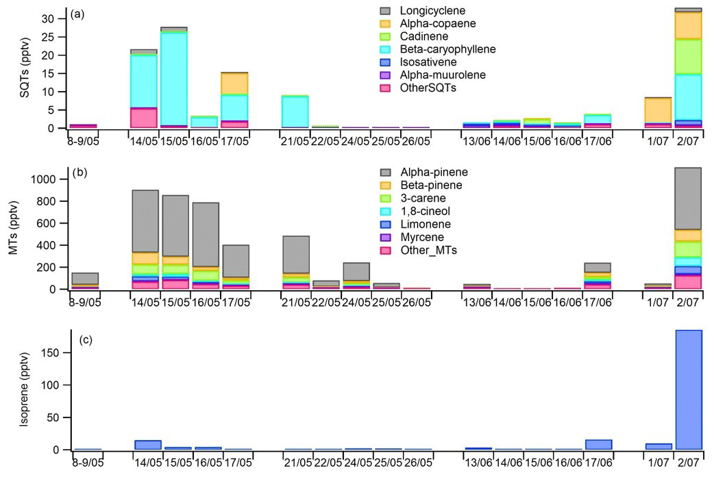
Figure 9 Daily mean concentrations of (a) sesquiterpenes (SQTs), (b) monoterpenes (MTs) and (c) isoprene in the ambient air at Lompolojänkkä fen in 2018.

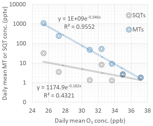
Figure 10 Dependence of daily mean ozone concentrations on daily mean monoterpene (MT) and sesquiterpene (SQT) concentrations during the ambient air measurements in June and July in 2018.

Based on the snow depth measurements at the site, there were still 22 cm of snow on 8 May, but on 12 May no snow was present anymore (Fig. 6). The highest daily means for both MTs and SQTs were measured during this snow melting and soil thawing period (Fig. 9). Aaltonen et al. (2012) have shown that VOCs produced under the snow cover, for example by microbes and decaying litter, remain in the snow cover with quite high concentrations and are released to the air when snow is melting and the ground thaws. Melting and thawing will most likely influence the surrounding forest emissions as well (Aalto et al., 2015). The MTs detected in ambient air were the same as were also detected in the emission measurements.

The SQTs measured in ambient air were not the same as those measured in the emissions of the fen, but the most abundant compounds in air were α-copaene and β-caryophyllene (Fig. 9). β-Caryophyllene is very fast-reacting compound; its lifetime is only a few minutes, and it was only minor fraction (< 2 %) of fen emissions. However, there can be differences between the measurement periods as shown in Table 2, and there were no parallel emission and ambient air measurements, but β-caryophyllene is also the main SQT in Scots pine and Norway spruce emissions (Tarvainen et al., 2005; Hakola et al., 2017). Therefore it is likely that the surrounding Scots pine and Norway spruce forests may also be an SQT source. Other possible nearby sources are mountain birches (Haapanala et al., 2009). In any case, this would need nearby and high β-caryophyllene emissions since its lifetime is only few minutes. Cadinene was the main SQT in the wetland emissions, and it was detected in ambient air too. The main MT found in the ambient air, α-pinene, is the most important MT both in wetland and forest emissions (Rinne et al., 2000; Tarvainen et al., 2005; Hakola et al., 2017).

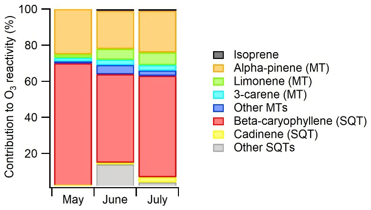
Figure 11 Contributions of various BVOCs to the ozone reactivity during the ambient air measurements at Lompolojänkkä fen in 2018. The reaction rate coefficients used are listed as Table S4.

The atmospheric concentrations are a mixture of emissions from the wetland and the surrounding forest. This explains why the most abundant VOC class were the MTs and not, for example, isoprene or SQTs, which were more highly emitted by the wetland. However, this comparison is not straight forward since isoprene is emitted only when daylight is available (Fig. 7), when the mixing layer of the atmosphere and therefore the dilution effect are also highest. MTs and SQTs are also emitted during the night, and at least in a southern boreal forest the highest concentrations of MTs and SQTs are often measured during the night when the mixing layer is very shallow even though daytime emissions are much higher (Hellén et al., 2018).

Generally, ambient air concentrations of SQTs and MTs in Lompolojänkkä were at the same level as measured earlier in a boreal forest in the Hyytiälä, southern Finland (Kontkanen et al., 2016; Hellén et al., 2018). However, in May the concentrations at Lompolojänkkä were higher than in Hyytiälä boreal forest. The mean MT concentration measured by Kontkanen et al. (2016) in May 2006–2013 in Hyytiälä was ∼150 pptv, and the SQT sum measured by Hellén et al. (2018) in May 2016 was 3 pptv, while at Lompolojänkkä MT and SQT concentrations in May were more than 2 times higher: 350 and 7 pptv, respectively (Table 2). Higher concentrations are not explained by the higher temperature. In Hyytiälä the mean temperature in May 2006–2013 was 10 ^∘C, which is the same as the mean temperature during our measurements in May at Lompolojänkkä, and during the SQT measurements in Hyytiälä in 2016 temperature was a bit higher (12.4 ^∘C). However, concentrations of terpenes are known to vary a lot even at the same site depending on the exact measurement point (Liebmann et al., 2018)

Vertical ozone fluxes measured above forests are explained at least partly by stomatal uptake and non-stomatal sinks, including chemical reactions with the BVOCs (Wolfe et al., 2011; Rannik et al., 2012). We found that daily mean MT and SQT concentrations had a negative exponential correlation with ozone concentrations as shown in Fig. 10. This indicates that BVOC emissions have a strong impact on ozone concentrations at this remote sub-Arctic site. However, the dependence was detected only in June and July. In May MT concentrations were highest, and no correlation was observed. The reason could be that during that time the main MT source impacting our measurements was very close by, perhaps in the snow cover on the fen as discussed earlier, while the impact of VOCs on ozone concentrations is a more regional phenomenon. In June and July, due to low emissions at the fen, the main source of MTs was expected to be more regional (e.g. surrounding forests). The lifetimes of MTs in relation to the ozone reaction are a few hours for most of the MTs (Hellén et al., 2018).

To estimate the effects of various BVOCs on local ozone chemistry we calculated ozone reactivities (R) of them by multiplying the measured concentrations with ozone reaction rate coefficients ($k_{{\mathrm{O}}_{\mathrm{3}}}$) as in Eq. (1).

$$\begin{array}{}\text{(1)}& R_i=\left[{\mathrm{BVOC}}_i\right]\times k_{i,{\mathrm{O}}_{\mathrm{3}}}\end{array}$$

The ozone reaction rate coefficients used were obtained from the literature and are listed as Table S4. This determines in an approximate manner the relative role of compounds or compound classes as an ozone sink. Of the measured compounds, SQTs had the highest (66 %) contribution, β-caryophyllene clearly being the most important SQT (Fig. 11). Isoprene had only < 1 % contribution. Of the MTs α-pinene and limonene had the highest contributions (23 % and 5 % of the total BVOC O₃ reactivity, respectively). The contribution of other compounds was minor. Since SQTs are highly reactive (lifetime of β-caryophyllene ∼2 min), their effect is very local, while MTs with a lifetime of a few hours have a more regional impact.

4 Conclusions

Emissions and ambient air concentrations of terpenoids were measured at the Lompolojänkkä fen in northern Finland in April–August 2018. Even though isoprene was the main terpenoid emitted from the fen and MT emissions were only 10 % of isoprene emissions, SQT emissions were several times higher than MT emissions, especially in early summer. Usually SQT emission from vegetation are several times lower than MT emissions. Emission rates of MTs were clearly lower than emission rates measured earlier at the nearby spruce forest (Rinne et al., 2000), but isoprene emission rates from the fen were clearly higher.

Changes in light and temperature conditions explained most of the seasonal changes in isoprene emissions. Isoprene emission rates also correlated well with the gross primary production of CO₂. The sesquiterpene emissions were partly controlled by other factors, which was seen, for example, as decreasing emission potentials over the growing season. High SQT emissions during early summer suggested that the compounds trapped in frozen soil and snow cover during winter could be an important source of these compounds when the soil is thawing.

Comparison with the emissions from a nearby forest indicated that the BVOC concentrations observed at the fen were not only affected by the fen emissions but also by emissions from surrounding ecosystems. Nevertheless, the wetlands were shown to be a significant source of isoprene within this kind of sub-Arctic landscape. Furthermore, strong correlation of daily mean ambient air concentrations of MTs and SQTs with ozone concentrations indicated that BVOC emissions from these ecosystems have a strong impact on the local ozone levels. Of the studied BVOCs, β-caryophyllene had the main contribution to local ozone reactivity.