Understanding nighttime methane signals at the Amazon Tall Tower Observatory (ATTO)

Methane (CH₄) atmospheric mixing ratio measurements are analyzed for the period between June 2013 and November 2018 at the Amazon Tall Tower Observatory (ATTO). We describe the seasonal and diurnal patterns of nighttime events in which CH₄ mixing ratios at the uppermost (79 m a.g.l.) inlet are significantly higher than the lowermost inlet (4 m a.g.l.) by 8 ppb or more. These nighttime events were found to be associated with a wind direction originating from the southeast and wind speeds between 2 and 5 m s⁻¹. We found that these events happen under specific nighttime atmospheric conditions when compared to other nights, exhibiting less variable sensible heat flux, low net radiation and a strong thermal stratification above the canopy. Our analysis indicates that even at wind speeds of 5.8 m s⁻¹ the turbulence intensity, given by the standard deviation of the vertical velocity, is suppressed to values lower than 0.3 m s⁻¹. Given these findings, we suggest that these nighttime CH₄ enhancements are advected from their source location by horizontal nonturbulent motions. The most likely source location is the Uatumã River, possibly influenced by dead stands of flooded forest trees that may be enhancing CH₄ emissions from those areas. Finally, biomass burning and the Amazon River were discarded as potential CH₄ sources.

1 Introduction

In the last decades atmospheric CH₄ has followed contrasting trends. Following decades of growth, during the period between 1999 and 2006, atmospheric CH₄ mixing ratios were stable (Dlugokencky et al., 2011), whereas during the last decade a steep growth has been reported (Nisbet et al., 2016). Currently the reasons for these trends are not clear and several explanations have been proposed (Nisbet et al., 2016; Schaefer et al., 2016; Turner et al., 2017; Rigby et al., 2017; Howarth, 2019). What is evident in the current debate is that CH₄ emissions from tropical wetlands are the single largest source of uncertainty to the global CH₄ budget (Kirschke et al., 2013; Saunois et al., 2016). Recent estimates suggest that Amazonian CH₄ emissions could contribute to about a third of the global wetland CH₄ emissions (Pangala et al., 2017). Therefore, better knowledge of the seasonal and diurnal dynamics of these emissions will provide valuable insights for developing process-based models that more accurately represent CH₄ emission and uptake (Turner et al., 2019). Our long-term measurements of CH₄ mixing ratios at the Amazon Tall Tower Observatory (ATTO) provide an opportunity for better understanding such seasonal and diurnal dynamics, which are necessarily linked to atmospheric transport (Gloor et al., 2001).

CH₄ is transported from surface sources, which in the Amazon are dominated by wetland ecosystems (Saunois et al., 2016; Wilson et al., 2016), to the upper levels of the troposphere. Therefore, the vertical profile of CH₄ mixing ratios in the troposphere generally decreases with height, showing higher mixing ratios in the boundary layer (Miller et al., 2007; Beck et al., 2012; Webb et al., 2016). The profiles discussed in previous studies have been based on airborne measurements taken at daytime under well-mixed conditions during specific campaigns (e.g., Beck et al., 2012) or during regular sampling programs with aircraft flights at least twice per month (e.g., Gatti et al., 2014; Webb et al., 2016). These studies provide valuable insights about regional atmospheric transport (Miller et al., 2007), spatial distribution of dominant CH₄ sources (Wilson et al., 2016) and the seasonal cycle across the Amazon region (Webb et al., 2016).

Closer to the surface, the proximity to the canopy and to the CH₄ sources becomes more important, dominating the variability of CH₄ mixing ratios at diurnal timescales. This strong variability is driven by a heterogeneous spatial distribution of sources (Gloor et al., 2001) and the complexity of atmospheric transport mechanisms in the first meters of the boundary layer (Stull, 1988). Despite these complexities, mixing ratio measurements close to the surface are the most feasible way to perform long-term measurements at high temporal resolution that can provide insights at diurnal and seasonal timescales. However, such types of measurements are sparse in this region, particularly for CH₄.

There are two studies that provide an idea of the diurnal variability of CH₄ mixing ratios in the Amazon region (Carmo et al., 2006; Querino et al., 2011). Both of these studies were conducted in upland forest sites, similar to the present study. Carmo et al. (2006) performed CH₄ mixing ratio measurements during the dry and wet seasons at three different sites in the Amazon. At all sites they focused their profile measurements on the canopy layer, which included one sampling inlet not more than 10 m above the canopy top. This study found that mixing ratios were generally higher at nighttime than during the day at all sites. As Carmo et al. (2006) focused on identifying local sources and calculating a local budget, the authors do not specify the amplitude of the diurnal cycle for the dry and wet seasons. Querino et al. (2011) provide one of the few records showing the diurnal variability of CH₄ above the canopy (53 m), as well as mixing ratio profiles within the canopy. CH₄ mixing ratios above the forest were higher during the night than during the day. The amplitude of the diurnal cycle was particularly large in July (>30 ppb), whereas in November there was no diurnal variability (Querino et al., 2011). Vertical CH₄ mixing ratios inside the canopy were found to decrease with height, during both day and night, but more strongly during nighttime measurements, agreeing with Carmo et al. (2006). Both Querino et al. (2011) and Carmo et al. (2006) attributed this feature to a source located in the soil, and they both concluded that the upland forest is a source of CH₄. The observed high nighttime CH₄ mixing ratios were explained by referring to a shallower nocturnal boundary layer that led to accumulation of CH₄ above the canopy (at 53 m) in Querino et al. (2011) and throughout the canopy layer in Carmo et al. (2006).

In the present study we describe similar nighttime CH₄ mixing ratio patterns using the unprecedented long-term measurements at ATTO. This unique dataset allows us to better describe the seasonal and diurnal variability of nighttime CH₄ signals at the 80 m tower. Furthermore, we provide a detailed analysis of the dominant atmospheric conditions under which high CH₄ mixing ratios are measured during the night at the top of the tower. Finally, we suggest possible sources of this nighttime CH₄ together with a description of the transport mechanisms that could be responsible for the vertical and horizontal transport of CH₄ in the nocturnal boundary layer.

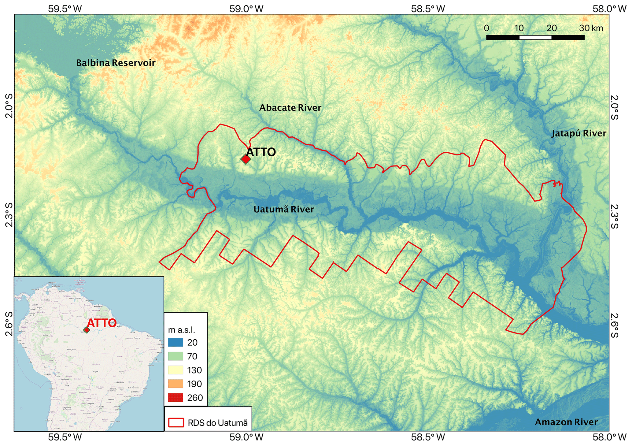
Figure 1 Location of ATTO relative to the continent. The topography, in the background, is based on the elevation model from the Shuttle Radar Topography Mission (NASA-JPL, 2013). The boundaries of the Uatumã Sustainable Development Reserve (USDR) are highlighted in the red polygon and the major rivers are labeled. Background layer of the inset map: ©OpenStreetMap contributors 2020. Distributed under a Creative Commons BY-SA License.

2 Data and methods

2.1 Site description

The Amazon Tall Tower Observatory (ATTO) research station is described in detail by Andreae et al. (2015); here we will only highlight aspects relevant to the current study. The ATTO site is located in the Uatumã Sustainable Development Reserve (USDR), which is 150 km northeast of the city of Manaus, in central Amazonia. The site was built on a plateau (130 m a.s.l.) surrounded by a large drainage network composed of depressions or valleys at lower elevation, which together with the plateaus form a small-scale heterogeneous topography with maximum height gradients of about 100 m (see Fig. 1).

The site is located in the interfluve between the Uatumã River and its tributary, the Abacate River. Both of these rivers flow in a NW to SE direction, merging their waters further southeast of the site. The flow of the Uatumã River is controlled by the Balbina reservoir, a hydroelectric dam located 55–60 km to the northwest of ATTO. The natural flood pulse of the Uatumã River was disturbed by the Balbina reservoir, causing a high level of tree mortality along the riverside (Assahira et al., 2017; Resende et al., 2019). It is worth noting that the Abacate River has not suffered hydrological disturbances, and still it presents a natural flooding seasonality.

The vegetation of the USDR is composed of different ecosystems. Upland dense forest (terra firme) is the characteristic vegetation on the plateaus and slopes, with the highest canopy, when compared to the surrounding valleys (Andreae et al., 2015). The canopy height at ATTO is around 37 m, but the mean canopy height over the plateau is 20.7±0.4 m (Andreae et al., 2015). In between the permanent flowing river channels and the terra firme forest, a savanna-type ecosystem on white-sand soil (campina) and forest on white-sand soil (campinarana) are found. In the campina there are smaller shrubs and trees with a vegetation height of 13.1±2 m. The campinarana has a canopy with emergent trees up until 17 m (Klein and Piedade, 2019). Along the Uatumã River and the Abacate River, seasonally flooded black-water forest (igapó) is the dominant type of vegetation (Andreae et al., 2015).

Figure 2 Monthly sums of precipitation for the period between 2013 and 2018 at ATTO.

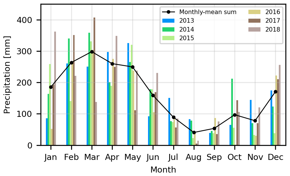
The regional atmospheric circulation has a seasonal pattern driven by the annual north–south shift of the Intertropical Convergence Zone (ITCZ) over the Atlantic Ocean (Andreae et al., 2012, 2015; Pöhlker et al., 2019). During the dry season, which we define here from July to October, ATTO is located south of the ITCZ. During the wet season, defined here from February to May, ATTO is located north of the ITCZ. This seasonal shift influences the origin of the air masses entering the continent and arriving at ATTO. During the dry season the prevailing wind direction is from the east, whereas the wind direction during the wet season is predominantly from the northeast (Andreae et al., 2015). Easterly winds during the dry season transport air masses containing signals from biomass burning, occurring mainly in the eastern part of the arc of deforestation in Brazil. The northeasterly winds during the wet season are transported over a large fetch of continuous rainforest, yet containing high background mixing ratios of greenhouse gases due to the influence of the Northern Hemisphere (Andreae et al., 2012, 2015). The dry and wet seasons were defined using precipitation data collected at the site with 30 min resolution covering a period from January 2013 to December 2018. The highest precipitation values are recorded from February to May, with a maximum of 300 mm month⁻¹ during March, while the lowest values, at below 100 mm month⁻¹, are found for the months between July and October (Fig. 2).

2.2 CH₄ mixing ratio sampling system

Our continuous measurements system was installed in March 2012 in the 80 m tall tower. This tower was built during the pilot phase of an ongoing measurement program. There are five air inlets located at 79, 53, 38, 24 and 4 m above ground. At these heights, we measure atmospheric mixing ratios of CH₄, carbon dioxide (CO₂) and carbon monoxide (CO) using two Picarro analyzers: the G1301 for CH₄ and CO₂ and the G1302 for CO₂ and CO. The G1301 analyzer (model CFADS-109) provides data with a standard deviation of the raw data below 0.05 ppm for CO₂ and 0.5 ppb for CH₄. For the G1302 (model CKADS-018), the standard deviation of the raw data is 0.04 ppm for CO₂ and 7 ppb for CO. For more details on precision and long-term drift, see Andreae et al. (2015). Similar to Winderlich et al. (2010), downstream of each sampling line 8 L stainless-steel spheres act as buffer volumes. This buffer system provides ideal air mixing characteristics to have continuous near-concurrent measurements at all heights (Winderlich et al., 2010). In Winderlich et al. (2010) the buffers integrate the air signal from every inlet with an e-folding time of approximately 37 min, with a flow of 150 sccm (standard cubic centimeter per minute) at 700 mbar. As we have two analyzers, our time resolution is higher with an e-folding time of approximately 18 min (8 L/(150×2) sccm at 700 mbar). Therefore, we assume that the 15 min averages used in Sect. 3.2.3 correspond to independent samples. The standard data, available at http://attodata.org (last access: 25 February 2020), are at 30 min resolution.

2.3 Meteorological instrumentation

For this study, we use wind direction, wind speed, air temperature, net radiation, precipitation and soil moisture. Sonic anemometers are fixed at 14, 22, 41, 55 and 81 m (above ground level; a.g.l.), but in this study we mainly use wind speed and direction at 81 m (Windmaster, Gill Instruments Limited). In Sect. 3.1 we show wind speed profiles for specific nights, using additional data from the sonic anemometers (model CSAT3, Campbell Scientific, Inc.) at 14, 41 and 55 m which perform fast response wind (u, v and w) measurements. At 81 m molar densities of CO₂ and H₂O are measured with an infrared gas analyzer (IRGA, LI-7500A, LI-COR Inc., USA). Air temperature is measured at 10 heights: 81, 73, 55, 40, 36, 26, 12, 4, 1.5 and 0.4 m (a.g.l.) with a termohygrometer (C215, Rotronic Measurement Solutions, UK). Net radiation is measured with a net radiometer (NR-Lite2, Kipp & Zonen, the Netherlands) at 75 m (a.g.l). For precipitation data, a rain gauge (TB4, Hydrological Services Pty. Ltd., Australia) is installed at 81 m, and for soil moisture a water content reflectometer (CS615, Campbell Scientific Inc., USA) provides data for the depths: 0.1, 0.2, 0.3, 0.4, 0.6 and 1 m.

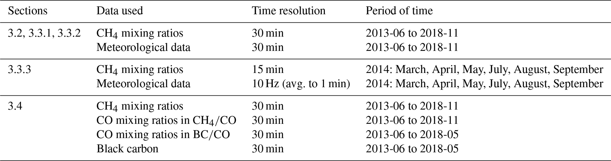
Table 1 Observational data used in each of the sections. We specify the time resolution and the period of time used.

2.4 Time period of data used

In the present study we have used CH₄ mixing ratio and meteorological data at different time resolutions. When mentioning meteorological data, we refer to the variables described in Sect. 2.3. To provide more clarity, we specify what type of data were used in each section. In Sect. 3.2, 3.3.1 and 3.3.2 we used CH₄ mixing ratios and meteorological variables at 30 min resolution. The CH₄ mixing ratio record covers the period from June 2013 to November 2018, which enabled us to study the diurnal and seasonal variability within this period. In Sect. 3.3.3, we used high-frequency (10 Hz) meteorological data, in particular all wind components (u, v and w), in order to associate turbulence regimes with CH₄ mixing ratios at 15 min resolution. More on the assumptions to link high-frequency wind data with 15 min mixing ratios is given below. In Sect. 3.4, we use 30 min averages of CH₄, CO and black carbon (BC) equivalent mass concentrations to assess the influence of biomass burning emissions in our CH₄ signals. The raw BC mass concentrations at 1 min time resolution were obtained using a multiangle absorption photometer (MAAP, model 5012, Thermo Fisher Scientific, Waltham, USA), as described in Saturno et al. (2018). The instrument measures the absorption coefficient of aerosol particles deposited on a filter, which is converted to BC mass concentration by assuming a mass absorption cross section of 6.6 m² g⁻¹. In Table 1, we provide a list of the data used in each section, specifying the time resolution and the period of time used.

2.5 CH₄ gradient definition

A CH₄ gradient is defined as CH₄${}_{\mathrm{grad}}={{\mathrm{CH}}_{\mathrm{4}}}_{\mathrm{79}\mathrm{m}}-{{\mathrm{CH}}_{\mathrm{4}}}_{\mathrm{4}\mathrm{m}}$. We indicate that the units of the CH_4grad and the comparisons here are in parts per billion (ppb). We refer to a positive gradient when CH_4grad>0 ppb or to a negative gradient when CH_4grad<0 ppb. Note that positive gradients are related to higher CH₄ mixing ratios at 79 m than at 4 m, while negative gradients to higher mixing ratios at 4 m. Throughout this paper we also use a 8 ppb threshold for classifying positive gradients and negative gradients. In Sect. 3.2 we use three classes. The first one refers to very strong positive gradients (CH_4grad>8 ppb or the above-8 ppb class), the second one refers to gradients in between −8 and 8 ppb ($-\mathrm{8}<$ CH_4grad<8 ppb) and the third one refers to very strong negative gradients (CH₄${}_{\mathrm{grad}}<-\mathrm{8}$ ppb). In Sect. 3.3, we have limited our analysis to two classes: CH_4grad>8 ppb and CH_4grad<8 ppb (the below-8 ppb class). The motivation to use 8 ppb as the threshold value is to leave out small mixing ratio variations and select very strong events. The ±8 ppb threshold is conservative and filters for strong gradients if we consider that the annual global increase in atmospheric CH₄ during the last 3 years was 7.06, 6.95 and 10.77 ppb yr⁻¹ for 2016, 2017 and 2018, respectively (Dlugokencky, 2019). It is always stated in the text which of these classes is being considered.

2.6 Analysis of 30 min averages

In Sect. 3.2, the 30 min averages of CH₄ mixing ratios were grouped into daytime and nighttime and further classified into the three classes as described in Sect. 2.5. In Sect. 3.3.1 strong CH₄ positive gradients were associated with wind direction by using the Openair package in R developed by Carslaw and Ropkins (2012). This R package provides useful predetermined functions to interpret air pollution characteristics based on wind speed, wind direction and other variables. Micrometeorological data were used together with co-located CH₄ mixing ratio data at ATTO (Sect. 3.3.2). The heights of the highest sonic anemometer and the highest air inlet for CH₄ mixing ratio measurements differ by 2 m, with the former at 81 m and the latter at 79 m. We assume that the effect of the 2 m can be neglected and thus interpret all the 81 m data as valid for 79 m. In order to maintain consistency, we used the same 8 ppb threshold as in Sect. 3.2, but this time we clustered the other two classes (CH₄${}_{\mathrm{grad}}<-\mathrm{8}$ ppb and $-\mathrm{8}<{{\mathrm{CH}}_{\mathrm{4}}}_{\mathrm{grad}}<\mathrm{8}$ ppb) into only one: the below-8 ppb class. The latter provides more clarity in the interpretation, as we are strictly interested in the above-8 ppb class.

2.7 Analysis of 1 min averages

In Sect. 3.3.3 we analyze the CH₄ positive gradients for the stable boundary layer taking into account the turbulence regimes defined by Sun et al. (2012). For this analysis, we use high-frequency data (10 Hz) for micrometeorological variables, but we averaged them to 1 min in order to be consistent with recent practice in nocturnal boundary layer studies (Marht et al., 2013; Acevedo et al., 2016, 2019) and to more strictly filter out low-frequency submesoscale fluctuations (i.e., nonturbulent motions at scales smaller than those at the mesoscale) (Mahrt, 2009) in all wind components. We focus on 6 months of 2014 (March, April, May, July, August and September). We have selected these months to target wet and dry seasons, and we discarded June because it is considered a transition month based on precipitation. These turbulence regimes are classified into two classes: the above-8 ppb and below-8 ppb classes. This classification is performed using the highest temporal resolution of CH₄ mixing ratio data, which is 15 min. We assume that the gradient is constant for each 15 min interval. For example, if the CH₄ gradient is 5 ppb at 21:00 LT (local time), we use the same value for every minute until 21:14 LT.

Figure 3 CH₄ time series for three selected nights (a–c), showing a 24 h interval, virtual potential temperature and mean wind profiles for three selected periods of the CH₄ time series. The times at which the profiles are plotted are highlighted on the CH₄ time series with the same colors. The canopy height is approximately 35 m. Note that due to the instrument malfunctioning the Θ_v profiles are lacking data at 12 m. The wind speed profiles cover from 19 to 81 m.

3 Results

3.1 Example of CH₄ gradient events

In Fig. 3a we show a night in which a very strong positive gradient occurred. After 00:00 LT and before 01:00 LT, there is a sudden and abrupt divergence of CH₄ mixing ratios measured at 79 m. This increase in CH₄ is not seen at the first three measurement levels, while at 53 m it is observed with some delay and with less intensity. The divergence at 79 m reaches a CH₄ peak of 1960 ppb at around 04:00 LT, at which point the lowest three inlets show CH₄ mixing ratios lower than 1880 ppb. At this time there is a strong thermal inversion for the air above the canopy, and the wind speed at 81 m decreases to almost 1 m s⁻¹. The duration of this positive gradient, considering the time in which the 79 m inlet had mixing ratios higher than 1880 ppb, was about 5 h. These positive gradient events are very common in our time series, and they vary mainly in duration and magnitude. For the case shown in Fig. 3a, we can see that the decoupling between the air above and within the canopy was very strong up until 53 m. At the 53 m level the signal, first measured at 79 m, arrived about 30 min later when the CH₄ mixing ratio began to increase, but at the lower levels the behavior is completely independent. Decoupled conditions can be explained by a very strong thermal inversion that obstructs vertical mixing, which could be triggered by wind shear under stable conditions (Mahrt, 2009).

For other cases in which we observed positive gradient events during nighttime, the signals measured at 79 m are then measured at the lowest inlet (4 m) after some time, varying from 30 min to 1.5 h (see Fig. 3b). For these situations, when the coherent response at the lowest levels is within the next half an hour, it could be explained by the sequential sampling (top-to-bottom) and the buffer volume in our measurement system. However, in the case of such a subsequent top-down signal, we also find that the decoupling between the air above and within the canopy is weaker or nonexistent.

The virtual potential temperature (Θ_v) profiles above the canopy at 22:00 and 02:00 LT show a very similar gradient with a weak thermal inversion. Interestingly, at 02:00 LT when the CH₄ mixing ratio at 79 m reached the maximum, the wind speed at 81 m decreased to 1 m s⁻¹, and for the same time the Θ_v profile showed a mild gradient of about 1.2 K. This mild temperature increase with height above 41 m indicates that the decoupling of the air above the forest is less strong, explaining why the CH₄ is measured subsequently at lower heights. Note that vertical transport for these situations is triggered by mechanical turbulence (generated by wind shear instabilities) or intermittent turbulence that, in the absence of a very strong thermal inversion, can transport CH₄ to the lower inlets and inside the canopy (Oliveira et al., 2018). During this night, the gradient was less pronounced and it lasted for less time than in the night shown in Fig. 3a.

In Fig. 3c a night in which no gradient was measured is shown. An almost constant Θ_v profile indicates the coupling of the air above the canopy for the three selected times of the night. The thermal gradient for the layer above the canopy is about 1.5 K. The CH₄ mixing ratios are very similar at all inlet heights for the full 24 h period. During this night the wind speed has both the largest values and the lowest variability during the course of the night. From these three cases, one can see that positive gradient events are associated with atmospheric stability and wind speed. However, as we show in Sect. 3.3.1, the wind speed is not necessarily always weak for positive gradients.

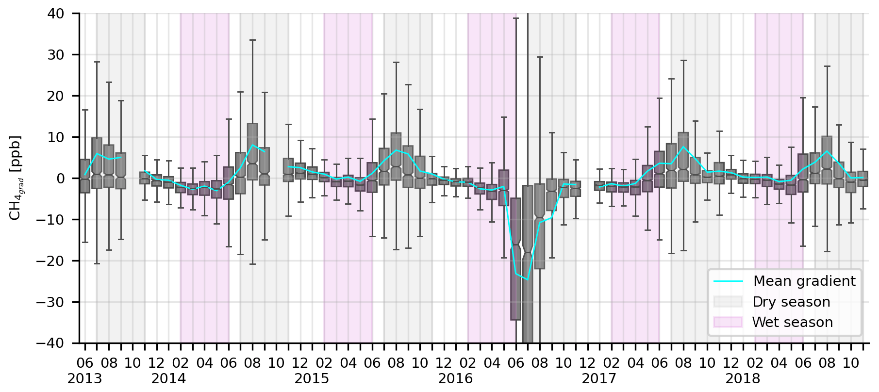
Figure 4 Box-and-whisker plot of monthly CH₄ gradients between the 79 and 4 m levels. The box denotes the interquartile range (IQR), showing the median with a notched line. The whiskers range from $Q_{\mathrm{1}}-\mathrm{1.5}\times$ IQR to $Q_{\mathrm{3}}+\mathrm{1.5}\times$ IQR, with Q₁ and Q₃ being the 25th and 75th percentiles. The cyan line is the monthly-mean gradient. The monthly statistics are calculated from half-hourly measurements at ATTO.

3.2 Seasonal and diurnal patterns of CH₄ gradients at ATTO

In Fig. 4 we show that for all years except 2016, monthly-mean positive CH₄ gradients (hereafter simply referred to as positive gradients) occur mainly during the dry season, whereas the mean gradient is close to zero during the wet season. The monthly-mean gradient is significantly different from zero during the dry months, with p values (two-sided t test) lower than 0.01. This positive gradient at ATTO is more pronounced during the month of August, when the lowest precipitation values are less than 50 mm (Fig. 2). A different behavior is observed for 2016, in which a strong negative gradient during June and July suggests a possible CH₄ source within the canopy measured at 4 m. The reason for this is unclear, yet we provide some ideas discussed later in this section. The dry season peak is also seen at the other measurement heights (not shown here), but at 79 m the measured CH₄ mixing ratios are the highest, indicating that nonlocal sources are predominant during this period of time. It is interesting to note that in the dry season also the largest variability in the gradient was observed, as opposed to the reduced variability during the wet season and transition months such as December and January.

The positive gradients observed during the dry season are associated with nighttime CH₄ mixing ratio peaks at 79 m. Figure 5 depicts the fraction of time for daytime and nighttime measurements for each of the classes described in Sect. 2.5. For all months, daytime measurements (Fig. 5a) are within the −8 to 8 ppb range over 60 % of the time. Gradients lower than −8 ppb or higher than 8 ppb are more frequent and increase their contribution to the total time during May, June, July, August and September. For these months, negative gradients are measured 8.7 %, 18.6 %, 22.3 %, 17.6 % and 7.8 % of the total daytime hours, while positive gradients are found for 3.6 %, 6.2 %, 10 %, 12.2 % and 8.4 %.

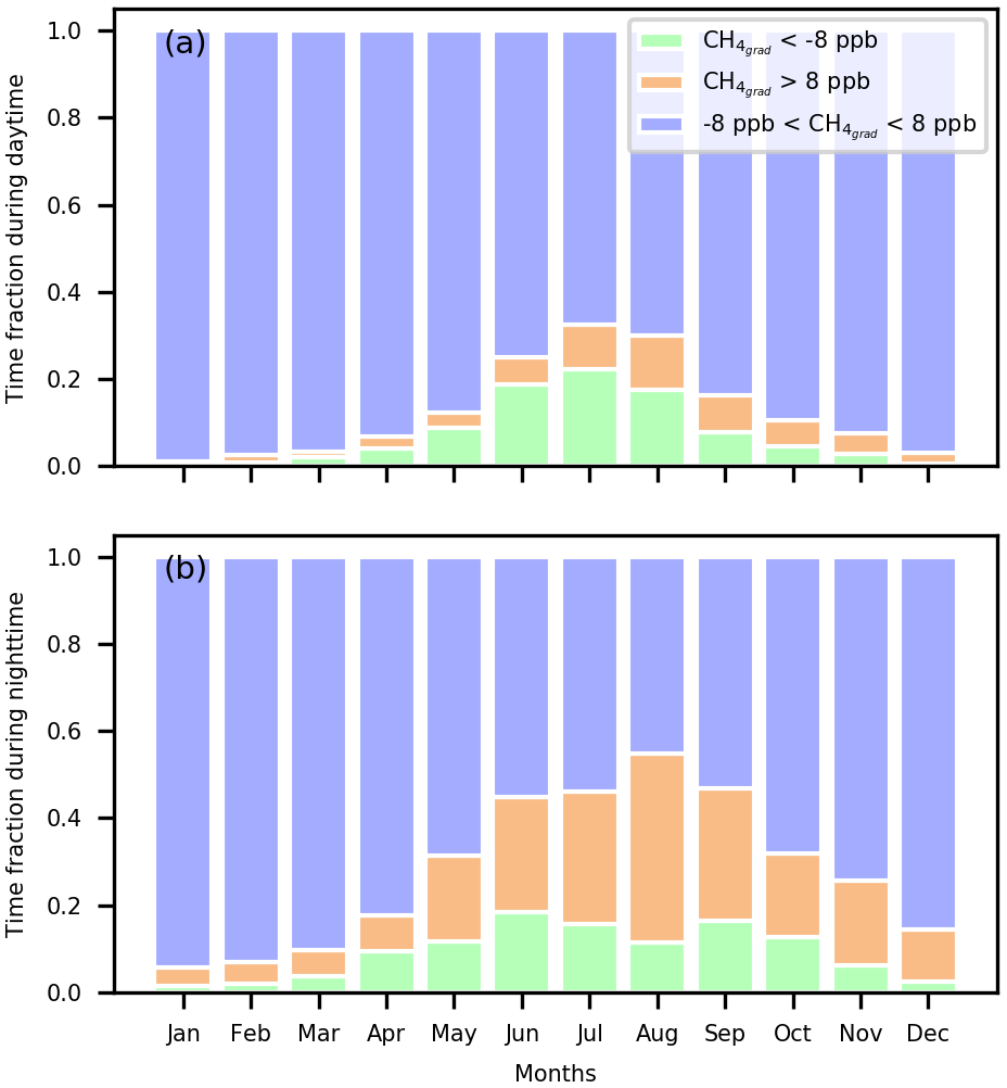
Figure 5 Time fractions for daytime (a) and nighttime (b) measurements in which CH_4grad>8, $-\mathrm{8}<{{\mathrm{CH}}_{\mathrm{4}}}_{\mathrm{grad}}<\mathrm{8}$ and CH₄${}_{\mathrm{grad}}<-\mathrm{8}$ ppb. Nighttime is defined as between 20:00 and 06:00 LT and daytime as between 07:00 and 18:00 LT (local time).

Nighttime measurements, in general, show a larger contribution of positive gradients to the total time (Fig. 5b). Nighttime positive gradients occur in all months of the year, from 4.1 % of the time in January to 43.3 % of the time in August. The highest percentages are recorded during the dry season months of July (30.2 %), August (43.3 %) and September (30.2 %). Unsurprisingly, these months also have the highest mean nighttime gradients, with 2.6±23, 9.7±21 and 6.2±23 ppb for July, August and September, respectively. The maximum nighttime positive gradients were observed between 03:00 and 06:00 LT (local time, not shown), with values larger than 130 ppb. During daytime, the maximum positive gradients occur between 07:00 and 08:00 LT, with values over 150 ppb. Note that these gradients are generated during nighttime and can persist for a couple of hours until the erosion of the nocturnal boundary layer and subsequent growth of the convective boundary layer, which occurs between 08:00 and 09:00 LT. (Fisch et al., 2004; Carneiro, 2018).

The mean diurnal cycles of the CH₄ gradient for dry and wet seasons provide interesting insights (Fig. 6). The amplitude of the mean diurnal cycle gradient during the dry season (12.1 ppb) is 4 times larger than that of the wet season (2.7 ppb). This substantial difference can be attributed to two main reasons. First, due to strong nighttime positive gradients during the dry season, the maximum mean (7.1 ppb) is much larger than the maximum mean of the wet season (0.5 ppb). Interestingly, both of these mean maxima occur at night, indicating that nighttime positive gradients are pulling up the mean in both seasons. Second, during the dry season the daytime planetary boundary layer is higher by a few hundred meters as a result of a larger sensible heat flux caused by the higher incoming shortwave radiation during this season (Fisch et al., 2004; Carneiro, 2018). Under this case with higher mixing ratios close to the surface and lower free tropospheric mixing ratios (as shown for dry and wet seasons by Beck et al., 2012), a deeper boundary layer directly affects daytime CH₄ mixing ratios, because CH₄ enhancements near the surface will be diluted in a larger volume. This dilution effect does not happen at the 4 m inlet, because the within-canopy air volume remains the same throughout the seasons. This boundary layer effect together with higher CH₄ mixing ratios at 4 m compared to 79 m during the dry season yields a lower dry season daytime mean minimum of −5.0 ppb, whereas the mean minimum during the wet season is −2.2 ppb.

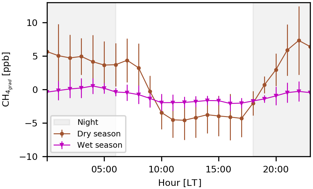
Figure 6 Mean diurnal cycle of the CH₄ gradient between the 79 and 4 m levels. The period between June 2013 and November 2018 was used and separated by dry and wet seasons. The error bars show the standard deviations.

Another possibility that might contribute to this seasonal difference is local production of CH₄ during the wet season. Though we lack long-term CH₄ flux measurements at the site, we can infer a potential local source during the wet season considering that the mean monthly gradient during daytime hours of the wet season is always negative (not shown), meaning that the CH₄ mixing ratio at 4 m is higher than at 79 m. Although outside of the scope of this study, strong negative gradients are more common during daytime, reaching differences as large as −455 ppb, measured in May 2014. The 4 m inlet is too high above the soil to directly associate this signal with the soil below, but it is well within the canopy, indicating that the source must be local and possibly within a horizontal distance of a few hundred meters. The event in May 2014 coincided with a strong signal measured for carbon monoxide (CO) with the same timing but not for carbon dioxide (CO₂), which suggests a source not related to combustion.

The mechanism producing this strong CH₄ signal within the canopy is currently under investigation, yet here we discuss what the potential sources could be. Our first thought is that the soil on the plateau is producing CH₄ episodically. Given some additional parameters, we can calculate the water-filled pore space (WFPS) for the depth (60 cm) of maximum soil moisture content, at which we believe CH₄ could be produced. To be conservative, we take the mean soil moisture value for the entire record at 60 cm: 0.35 m³ m⁻³. According to Andreae et al. (2015), 85 % of the soil in the plateau is clay, and thus we use a soil particle density of 2.86 g cm⁻³ (Schjønning et al., 2017). Also from Andreae et al. (2015), we use a bulk density of 1.1 g cm⁻³. This results in a WFPS of 57 %, which is likely to enhance the abundance of anaerobic microsites where methanogenic bacteria can be activated. At values above 60 % Verchot et al. (2000) found positive CH₄ fluxes; at the ATTO site values above 60 % are often seen during the wet season. Upland terra firme soils are generally considered CH₄ sinks (Dörr et al., 1993; Dutaur and Verchot, 2007; Saunois et al., 2016), but at local scales the soil can become a source depending on the balance between CH₄ production and oxidation (Verchot et al., 2000). Moreover, tree stems were found to play an important role as conduits for soil-generated CH₄ in upland terra firme tropical forest (Welch et al., 2019). These findings, together with our data, suggest that the upland terra firme CH₄ sink at ATTO needs to be further studied.

A second option is related to daytime anabatic flows within the canopy transported from the depressions to the plateau (Tóta et al., 2012). These anabatic flows could transport CH₄ produced in saturated soils of these low-lying areas. Recent (May 2019) unpublished CH₄ mixing ratio measurements suggest a possible source at the lowest point of one depression close to the ATTO site. A further possibility, not likely explaining the complete signal at 4 m but probably contributing to it, might be termite production within the canopy. Termite CH₄ production is common in tropical ecosystems (Sanderson, 1996); however, flux measurements from this source have not been performed at the site. The 2016 episode mentioned earlier provides evidence that CH₄ mixing ratios at 4 m could be strongly enhanced by unidentified processes that need further research. The natural variability of upland terra firme CH₄ sources or sinks could have been altered by the El Niño event that began in 2015 and lasted until early 2016, as shown by Pfannerstill et al. (2018) for OH at the ATTO site. For these episodes, which occurred during June and July (see Fig. 4), the enhancement at 4 m lasted for more than 5 h, presenting the onset at nighttime and maintained during daytime. Furthermore, the air within the 4 m layer above the ground seemed to be strongly decoupled from the layers above as none of the upper inlets measured the signal observed at 4 m (not shown). Therefore, the 4 m episodes described here are very likely a combination of an enhanced source and the stability conditions of the air within the canopy for those specific dates.

Figure 7 Mean CH₄ gradient for each bin of wind direction and time of day (a) or month of the year (b). Wind direction measured at 81 m and CH₄ mixing ratios at 79 m. Plot produced in R with the Openair package (Carslaw et al., 2010).

3.3 Atmospheric characteristics of positive CH₄ gradients

3.3.1 CH₄ positive gradients and wind direction for 2013–2018

For hourly timescales, we find that for nighttime hours and when the mean CH_4grad is above 8 ppb the wind direction is within the range of 90 and 180^∘ (hereafter referred to as southeasterly) (Fig. 7a, left panel). Note that the wind directions ranging between 180 and 270^∘, hereafter southwesterly, also show positive mean CH_4grad during nighttime hours, but these are lower than those seen when the wind comes from the southeast. For lower or negative mean CH₄ gradients and other times of the day, mainly daytime, the wind direction does not show a dominant pattern.

At monthly timescales we observed similar behavior, with a dominant southeasterly wind direction for mean CH_4grad above 8 ppb and the dry season months of August and September. During August and September, the southwesterly direction shows mean CH_4grad above 4 ppb, suggesting that this wind direction plays an important role in the positive CH_4grad events. Yet, it is very clear that large positive CH_4grad gradients are mainly driven by southeasterly winds. During dry season months the wind is more frequently coming from the east, whereas during the wet season there is a shift to northeasterly winds. In situ measurements of wind direction confirm this pattern. The monthly-mean wind roses (see Fig. A1) show that the wind is more frequently coming from the east and it is more likely to bring air masses from southeastern areas of ATTO during June, July, August and September. These months have wind direction frequencies close to 20 % with wind speeds ranging from 1 to 7 m s⁻¹. The mean wind rose plots for each hour of the diurnal cycle (see Fig. A2) indicate that after 15:00 LT the wind directions in the 90–180^∘ quadrant become more important than in previous hours of the day, with frequencies of about 15 %. After 18:00 LT, the frequency increases at this wind direction until 23:00 LT. These wind direction patterns together with the prevailing wind direction for the positive CH_4grad suggest that nighttime positive gradients are more frequent in the dry season due to the prevailing wind direction, being more likely to bring air masses from the potential source region located to the southeast of ATTO.

Figure 8 Polar plot showing the conditional probability function (CPF) of the gradients above 8 ppb (88th to 100th percentiles, shown in the bottom of the graph as 8 to 195). The radial axis shows wind speed intervals and the colors the probability of having gradient above the 88th percentile. This is shown for each bin composed by wind direction and wind speed at 81 m. Plot produced in R with the Openair package (Carslaw et al., 2010).

The probability of measuring gradients above the 88th percentile (8 ppb) together with wind direction and wind speed at 81 m is shown in Fig. 8. The highest probability (50 %) of having a gradient above 8 ppb is associated with a particular wind speed range: mainly from 4 to 5 m s⁻¹. This wind speed range is seen for different wind directions, with the two southern quadrants (from 90 to 270^∘) having a very similar probability of 40 % to 50 %, with a slightly higher conditional probability in the southeastern quadrant than the southwestern quadrant. For the northwest quadrant (270 to 360^∘), the probability observed is lower than 40 %, but interestingly the wind speed range holds. Therefore, the gradients above 8 ppb are associated not only with a range of wind directions but also with a particular wind speed range. We showed previously that southeasterly winds are clearly bringing CH₄-enriched air masses, but there is also a 40 % probability of having these enhancements (above 8 ppb) when the wind direction shifts to the southwesterly direction and also when it comes from the northwest with approximately 25 % probability at wind speeds of 5 m s⁻¹. It is relevant to note that 68 % of the positive CH_4grad occurs at wind speeds between 2 and 5 m s⁻¹ (not shown), which in the southern quadrants still have a higher probability of occurrence.

Considering these results, we can infer that dominant large-scale circulation patterns explain why large positive CH₄ gradients are more common during the dry season months. Thus, the wind arriving at ATTO is more likely to come from the source areas to the south of the site. Moreover, this also explains why large positive CH₄ gradients are more strongly associated with the southeasterly direction; wind direction frequency is larger for these months than for other months of the year. Large positive CH₄ gradients can also come from other wind directions, but they are less frequent. Therefore, we identify a potential source of the nighttime signals with a probability of 40 % to 50 % to the south of the ATTO site (see Fig. 8). Here it is important to recall that these percentages are based on the conservative threshold of 8 ppb; analyses not shown here using a lower threshold yield higher probabilities. The nighttime average wind direction is more frequently coming from the southeast, explaining why positive CH_4grad gradients are more strongly associated with these wind directions at this timescale.

Figure 9 Box-and-whisker plots of net radiation (a), sensible heat flux (b), friction velocity (c) and virtual potential temperature difference (d) for nighttime hours. At each hour the gray colors indicate data points that correspond to either a gradient above 8 ppb or below 8 ppb. The means are indicated by the green triangles, and the number of data points for each box-and-whisker plot is shown on the top of each panel. Note that the sensible heat flux and the friction velocity were measured at 81 m and net radiation at 75 m. Note that the air inlet for CH₄ mole ratios is at 79 m.

3.3.2 Net radiation, sensible heat flux, friction velocity and thermal stratification for CH₄ positive gradients for 2013–2018

Net radiation for the above-8 ppb class is more negative, indicating a stronger radiative cooling at ATTO (see Fig. 9a) when these episodes occur. Net radiation is less variable for positive gradients with lower mean and median values for all night hours. This can be explained because positive gradients are more frequent during the dry season and in particular in August when there is less cloud cover, as can be inferred by our precipitation record (Fig. 2), and as reported in Andreae et al. (2015). Clear skies contribute with a more effective radiative cooling at the canopy top, leading to a stronger thermal inversion in the nocturnal boundary layer (NBL). Net radiation estimates at ATTO provide indirect evidence that suggest a shallower NBL height during the dry season. Values above the canopy are more negative during the dry season than during the wet season (see Fig. B1), suggesting a strong thermal inversion driven by large nighttime radiative cooling at the top of the canopy. For stable nights at the ATTO site, Oliveira et al. (2018) found that at 81 m the turbulent fluxes were clearly less variable than at lower heights, indicating a very shallow NBL height.

The above-8 ppb class is associated with a less variable H (see Fig. 9b), tending to values close to zero. For this class, the mean and median values of H at the beginning of the night hours, mainly from 20:00 to 23:00 LT, are slightly more negative than for the other class. After midnight these values tend to be closer to zero for the above-8 ppb class, suggesting that the nocturnal boundary layer is more stable for positive gradient events. The variability of both classes between 20:00 and 23:00 LT is not as different as for the rest of the hours but still is slightly lower for the above-8 ppb class. Considering the height at which the H is zero, a proxy to infer the NBL height, one could say that positive CH₄ gradient events are associated with a very shallow nocturnal boundary layer (close to 81 m). The seasonal difference in NBL height was studied by Carneiro (2018) during the GoAmazon campaign (Martin et al., 2016), using a ceilometer, a lidar and a sonic detection and ranging instrument among other instruments. Carneiro (2018) found that the time to erode (total erosion is considered to be when sensible heat flux and net radiation become positive) the nocturnal boundary layer is larger during the wet season, suggesting a deeper NBL height as one of the reasons to explain this. It is worth noting that the ceilometer sensitivity differs between instruments and it can also be affected by changes in the background radiation (Wiegner and Geiß, 2012). The ceilometer used by Carneiro (2018) is a CL31 (Vaisala Inc., Finland) and the one at ATTO is a Jenoptik CHM15kx, used recently by Dias-Júnior et al. (2019) to determine the mixing layer depth using only daytime backscatter profiles. In another study with the Jenoptik CHM15kx, Wiegner and Geiß (2012) found that the lowest detectable mixing height is around 150 m; therefore, nights with a NBL height lower than this might not be well captured. Furthermore, the Carneiro (2018) study was conducted over pasture which has different roughness and radiative characteristics compared to old-growth forest, and as such the results cannot be extrapolated to ATTO. Nonetheless the study provides valuable information about seasonal differences in the NBL height.

Positive gradients are also associated with low friction velocity (u_*) variability as well as low mean and median values for all nighttime hours (see Fig. 9c). As a measure of mechanical turbulence, low u_* values suggest that positive gradients occur mainly at low turbulence intensity. This finding is not surprising as strong stability and the absence of turbulence can lead to accumulation of trace gases in the NBL (Stull, 1988; Fitzjarrald and Moore, 1990) due to reduced vertical mixing. However, under this common assumption and considering that the NBL above the canopy can attain shallow depths, one would expect to measure the accumulation of trace gases at least at the other inlet heights above the canopy or at inlet heights closer to the canopy, where the possible source could be located, but for many of these events this is not the case. The CH₄ signal that arrives at the uppermost inlet (79 m), driving a positive gradient, is often not seen at lower inlets. This is very often the case for the inlet at 38 m but less so for that at 53 m, indicating that the CH₄-rich air is advected within a layer that includes the 79 m inlet and sometimes the 53 m inlet but not those below 53 m. Having low friction velocity values and considering that the dominant wind speeds at which positive gradients have more probability of occurrence are between 2 and 5 m s⁻¹ (see Fig. 8) suggest that CH₄ signals are transported mainly by horizontal nonturbulent motions, which are probably formed by inactive turbulence mainly seen at the upper layers of the NBL. Such inactive turbulence contributes very little to the generation of turbulence as was indicated by Högström (1990).

The difference of Θ_v between 81 and 36 m is slightly higher for the above-8 ppb class than for the below-8 ppb class (see Fig. 9d). The difference between the median values of the two classes is approximately 0.5 K for all night hours, hinting at relatively faster radiative cooling at the top of the canopy for the above-8 ppb class. The variability of this difference is very similar between both classes; although, the above-8 ppb class is more skewed towards positive values. The difference between mean and median values for both classes is small, but the fact that we see a systematic difference at all night hours strengthens the argument that thermal stratification is stronger when positive gradients occur than for the other class.

3.3.3 Association of positive CH₄ gradients and NBL turbulence regimes

We have defined the NBL turbulence regimes following the work by Sun et al. (2012), which was further applied by Dias-Junior et al. (2017) at another site within the Amazon forest. In regime 1, turbulence is produced by local shear at low wind speed and low σ_w. In regime 2, σ_w increases with wind speed and bulk shear in the NBL triggers turbulence (Sun et al., 2012). In Fig. 10a the standard deviation of the vertical velocity (σ_w) is plotted as a function of mean horizontal wind speed (U) for all the data available in 2014 without differentiating between gradient classes. Here, one can see that the regime transition (between regimes 1 and 2) occurs at the wind speed bin of 5.8 m s⁻¹, which comprises the range between 5.6 and 6.0 m s⁻¹. At this threshold the uppermost quartile of σ_w exceeds 0.5 m s⁻¹, and the slope defined by median values changes notably. Therefore, we define this bin as the wind speed threshold that marks the transition from regime 1 to regime 2. Subdividing this further into the gradient classes above and below 8 ppb (Fig. 10b), we observe that the variability of σ_w close to the wind speed threshold (bins 5.8 and 6.5 m s⁻¹) is reduced for the above-8 ppb class. The upper quartile of σ_w for the above-8 ppb class exceeds 0.5 m s⁻¹ only up to 6.5 m s⁻¹. The median σ_w for both classes displays a similar range of variability at 7.5 m s⁻¹. The above-8 ppb class has a different distribution in the same wind speed bins close to the wind speed threshold, having lower median values of σ_w. This finding implies that vertical motions are even more suppressed at 81 m for the above-8 ppb class, regardless of the wind speed exceeding the threshold value.

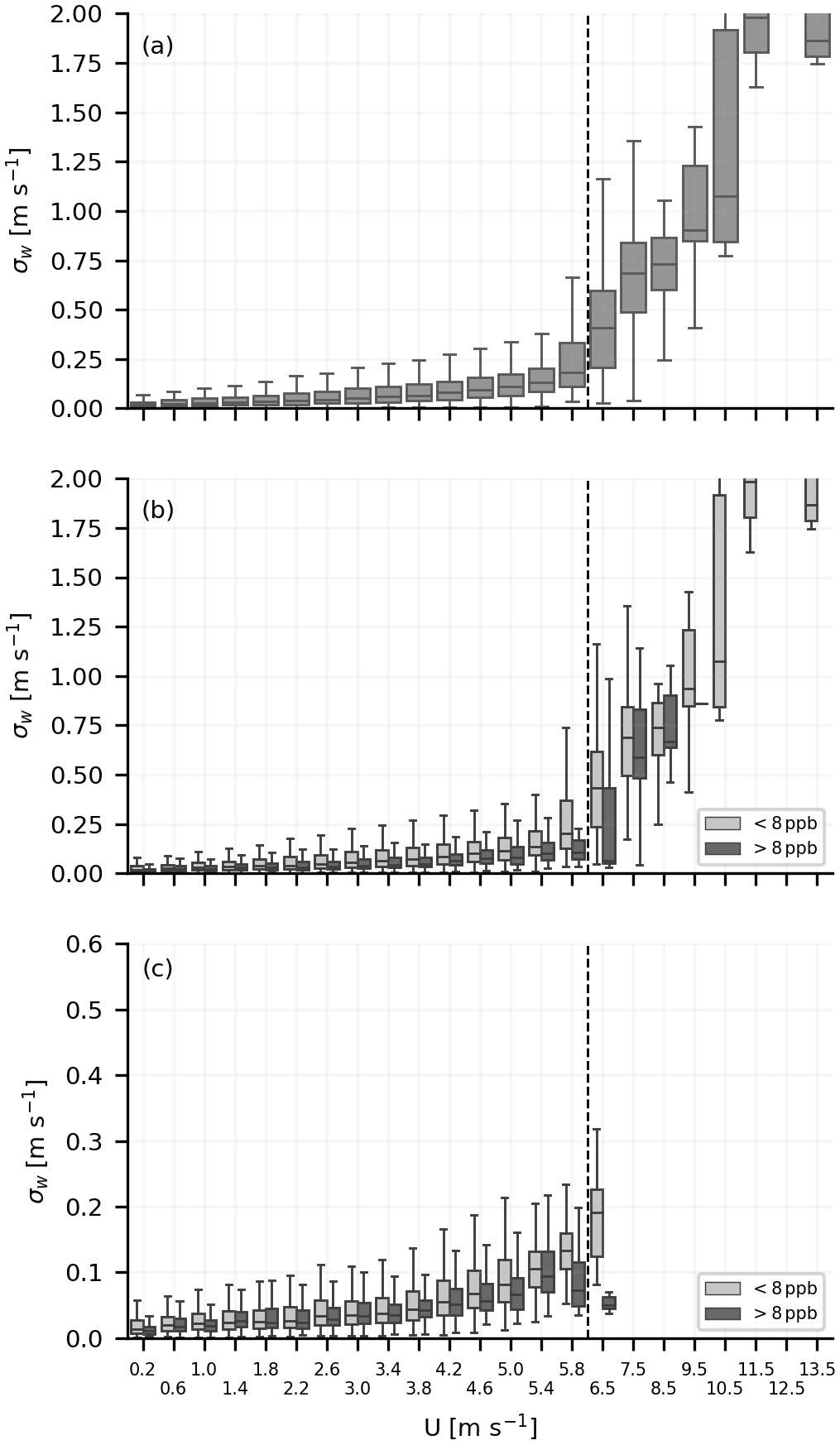
Figure 10 Standard deviation (σ_w) of the vertical velocity, plotted against the mean wind speed, for 1 min averaging time. In the top panel (a), the variability of σ_w for each wind speed bin is shown for all data points, with no classification based on CH₄ gradients. In (b), the same as (a) is shown but separating between measurements with gradients above and below 8 ppb. Note that our CH₄ mixing ratio measurements are at 15 min resolution; therefore, we assume the same value every 15 min window, so we can associate the 1 min σ_w and U with CH₄ mixing ratios. In the bottom panel (c), we excluded the 15 min time periods where the wind speed varied by more than 0.5 m s⁻¹. Note the difference in y axis for (c). The wind speed bins are shown every 0.4 m s⁻¹ until 5.8 m s⁻¹ and after the spacing is 1 m s⁻¹. This gradual increase to coarser wind speed bins is done due to less data at higher wind speeds. High-frequency measurements cover six months of 2014: March, April, May, July, August and September.

Given these facts, we can associate positive gradients with the more stable regime 1: low σ_w even at wind speeds exceeding the threshold value, identified without separating into gradient classes. In other words, the wind speed threshold under positive gradient events is shifted to a higher wind speed, maintaining low σ_w values. To account for wind speed variations that could affect our assumption of constant CH₄ mixing ratios for every 15 min window, we have filtered out the 15 min time periods in which the difference between the maximum and minimum wind speed is larger than 0.5 m s⁻¹ (Fig. 10c). After filtering, the dependence of σ_w on wind speed shows a similar pattern for each of the classes. In general, σ_w is less variable for positive gradient events. However, the difference in wind speed threshold is even more evident at the wind speed bins of 5.9 and 6.1 m s⁻¹. According to Sun et al. (2012), turbulence in regime 1 is weak and is controlled by vertical temperature gradients, in line with our finding of a stronger thermal stratification for positive gradients shown before. In regime 1 eddies generated at the observation height triggered by local shear do not come into contact with the ground (Sun et al., 2012). This is because, as stated by Sun et al. (2012), the length scale of the local shear is smaller than the observation height.

More evidence about the dominant regime of the NBL when the positive gradients occur is given by the potential temperature gradient ($\frac{\mathrm{d}\mathit{\theta }}{\mathrm{d}z}$) between 81 and 36 m. We found that 99.95 % of the positive gradients occur with positive values of $\frac{\mathrm{d}\mathit{\theta }}{\mathrm{d}z}$. As a result, one can infer the absence of vertical motions at the tower location. We can only attribute this lack of vertical mixing above the canopy to the tower location. Therefore, we have to separate the NBL conditions at the tower and at the potential source location. Unfortunately, we only have measurements at the tower and it is not realistic to measure at all possible source locations. Thus, the transport mechanisms can be divided into (1) those responsible for vertical transport of CH₄ at the source location and (2) those responsible for the horizontal advection bringing the CH₄ signals to the tower. More on the vertical and horizontal transport mechanisms is discussed in Sect. 4.2.

3.4 Rejecting biomass burning and the Amazon River as potential sources

The timing of the biomass burning season coincides with the dry season in the Amazon region (Gatti et al., 2014; van der Laan-Luijkx et al., 2015; Aragão et al., 2018), thus one could think that CH₄ from combustion is responsible for the positive gradients presented here. During incomplete combustion, CH₄ is co-emitted together with carbon monoxide (CO) (Akagi et al., 2011; Kirschke et al., 2013; Andreae, 2019); thus, CO is considered a good proxy for biomass burning and it can be used as a reference to get an idea of enhancement ratios due to fire emissions.

In Fig. 11 large CO mixing ratios (>200 ppb) are observed, suggesting that for these measurements we could have sampled air with biomass burning signals. However, these data points represent only 10 % of the data shown. Moreover, biomass burning typically produces CH₄ in a certain emission ratio to CO, dependent on the fuel type (Andreae and Merlet, 2001; Andreae, 2019). These reference ratios are shown as lines in Fig. 11 and it can be seen that very few points fall on the reference lines and the CH₄ mixing ratios are substantially enhanced compared to those of CO, indicating an additional source of CH₄ seen for all wind directions. The mean CO mixing ratio during nighttime in the dry season at 79 m (140±1.6 ppb) is on average 33 ppb higher than during the wet season (107±1.25 ppb), suggesting that during the dry season we observe a “background enhancement” of CO mixing ratios at ATTO. Therefore, we can conclude that CH₄ measurements at ATTO during the dry season will always have a contribution of biomass burning, but as Fig. 11 shows this background enhancement of CO can not completely explain the additional CH₄ of the positive gradients. Note that most of the data points are grouped below 200 ppb for CO, suggesting that positive gradients occur with CO mixing ratios close to the mean dry season mixing ratio. Given these facts, we believe that positive gradients have a minor contribution of CH₄ from biomass burning, but the magnitude of the CH₄ enhancement relative to the CO mixing ratios needs to have an additional source.

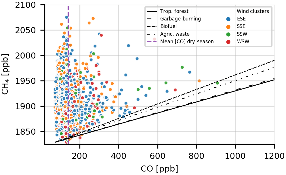
Figure 11 Methane (CH₄) as a function of carbon monoxide (CO) together with the slopes of the expected emission ratios (ER) for different types of fires based on the updated assessment of Andreae (2019) and classified into the dominant wind direction clusters for positive gradients (southern quadrants: from 90 to 270^∘). The data points were filtered to select only nighttime measurements, and the CO data were further filtered to select the same times for which the above-8 ppb class was seen for our CH₄ mixing ratio measurements. The data cover the time period between June 2013 and November 2018. All measurements were performed at 79 m.

Therefore, the challenge constraining to what extent fire emissions affect our CH₄ relies on identifying a clear and distinctive fire plume that provides information on not only the CH₄∕CO ratio but also the ratio relative to other species. Considering that black carbon (BC) particles are emitted in smoldering and flaming fires (Andreae and Merlet, 2001) together with CO and CH₄, we use BC measurements to gain more insights about the influence of fire emissions on the full CH₄ signal at ATTO. Following the same approach as in Fig. 11, the BC∕CO ratios in Fig. 12 indicate a more clear fire signal for the ESE and SSE wind directions. Note that the time period used in this plot is 5 months shorter than in Fig. 11 and contains fewer data points, yet some of those points fall on the reference slopes of Andreae (2019). In general terms, even though fire signals are measured at ATTO during nighttime for positive CH₄ gradients as suggested by Fig. 12, the nighttime CH₄ enhancements at 79 m are not fully explained by combustion. Most of the data points in the ESE wind direction match the reference slope for biofuel and tropical forest burning. Both of these are linked to human activity, and according to the comprehensive study by Pöhlker et al. (2019) in the ESE direction there is substantial fire activity, the rainforest has suffered more fragmentation and degradation, and there are more settlements. It is worth recalling that here we are focusing on nighttime data when stable atmospheric conditions prevail; therefore, the BC associated with biofuel burning might come from nearby settlements. For other directions, the fire signal is not so evident, and for some data points the CO mixing ratio is very high. This can be seen for all wind directions, and we believe that this can be explained by a possible weakening of the BC∕CO ratio due to deposition of BC (Saturno et al., 2018). Last but not least, even though biomass burning takes place throughout the entire dry season, its influence at the ATTO site is more relevant during October and November, as shown by Saturno et al. (2018) and our carbon monoxide time series. Despite being able to detect a clear fire signature, CH₄ enhancements are too high relative to CO, suggesting that an additional source is needed to explain the positive CH₄ gradient enhancement during nighttime.

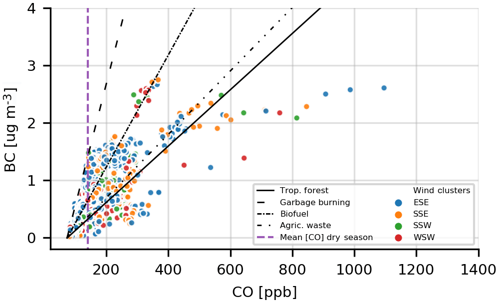
Figure 12 Black Carbon (BC) as a function of carbon monoxide (CO) together with the slopes of the expected emission ratios (ER) for different types of fires based on the updated assessment of Andreae (2019) and classified into the dominant wind direction clusters for positive gradients (southern quadrants: from 90 to 270^∘). The data points were filtered to select only nighttime measurements, and the BC data were further filtered to select the same periods at which the above-8 ppb class was seen for our CH₄ mixing ratio measurements. Note that the BC dataset spans from June 2013 to May 2018. The heights of CO and BC measurements are 79 and 60 m a.g.l., respectively.

The Amazon River was discarded as a potential source even though it coincides with the wind direction found for the positive gradients. The Amazon River is 120 km southeast of ATTO, which means that a strong CH₄ emission into the nocturnal boundary layer will have to be advected at a wind speed of 6 m s⁻¹ to reach ATTO in 5 h. This might be possible on some occasions but as we saw before (Fig. 8) positive gradients are associated with wind speeds between 2 and 5 m s⁻¹. Moreover, 80 % of the wind speed for nighttime positive gradients is below 4 m s⁻¹. In addition, we calculated the distance to the CH₄ source by time integrating the wind speed at 81 m from 20:00 LT (beginning of the night) until the first occurrence of a positive gradient (>8 ppb). The distribution of these distances is shown in Fig. 13. The distances with more counts are below 50 km, 90 % of the data points fall below 100 km and 80 % of the data points are below 72 km. Given these facts, the Amazon River is not considered a potential source for the nighttime CH₄ positive gradients.

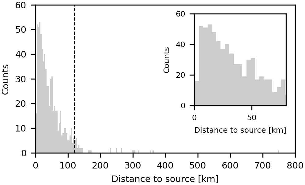
Figure 13 Distribution of the cumulative distance the wind at 81 m traveled from the potential source. The distance was calculated by time integrating the wind speed at 81 m from 20:00 LT (beginning of the night) until the first occurrence of a positive gradient (>8 ppb). The vertical dashed line shows the distance to the Amazon River in the southeast direction. The inset on the top right is a zoomed-in view showing the x axis until 80 km.

4 Discussion

4.1 Constraining potential nighttime CH₄ sources

Based on the predominant wind direction of the positive gradients, we propose a potential source of the nighttime CH₄ signals at the 79 m level. First in importance and most dominant is the southeastern quadrant, and second in line is the southwestern quadrant (see Figs. 7 and 8). In these directions lies the Uatumã River, which we believe is the most likely main source (but not unique) of the positive gradients seen at ATTO. In addition to the natural CH₄ production by this river, there are two additional sources that could enhance CH₄ degassing from this water body. The first one is related to an enhanced CH₄ concentration downstream of the Balbina reservoir. As it was shown by Kemenes et al. (2007), the Balbina reservoir not only leaks methane at the turbine intake due to depressurization but it also enhances CH₄ concentrations downstream along the Uatumã River. Kemenes et al. (2007) found that CH₄ concentrations in the Uatumã River decreased gradually until 30 km below the Balbina reservoir and remained constant for the next 70 km. It is worth noting that the CH₄ concentrations in the river were on average 24 µM (Kemenes et al., 2007), 3 orders of magnitude higher than the average background value (0.05 µM) for Amazonian rivers (Richey et al., 1988; Kemenes et al., 2007). The second additional source is very likely decomposition of dead flooded forest stands downstream of the Balbina reservoir along the Uatumã River. The dead stands are a consequence of the Balbina damming, which has changed the natural flooding pulse along the river, causing massive mortality of flooded forest trees along a 80 km stretch downstream of the dam (Resende et al., 2019). These dead stands were mapped recently by Resende et al. (2019), and their spatial distribution coincides with the wind directions associated with the positive gradient events (see Fig. C1). Rivers also emit carbon dioxide (CO₂), but the CH₄ enhancements described here do not coincide with an increase in CO₂. This is mainly because nighttime respiration is very strong and any nonlocal enhancement at 79 m is masked by local CO₂ signals at lower levels.

In addition, CH₄ could also be produced in the topographic depressions or valleys that form the drainage network surrounding ATTO. We have mentioned earlier that unpublished measurements of atmospheric CH₄ mixing ratios performed recently in one of these valleys indicate a nighttime increase in CH₄ within the canopy. Based on Junk et al. (2011), these depressions can be classified as wetlands subjected to unpredictable, polymodal flood pulses fed by rainwater, with low nutrient availability compared to the plateaus. The flooding dynamics are driven by flash flood pulses after precipitation events, which can flush out a large amount of the organic material available for decomposition (Florian Wittmann, 2019, personal communication). Therefore, these depressions were assumed to have low potential for producing CH₄. Nevertheless, the accumulation seen for CH₄ mixing ratio measurements performed during May and June in 2019 indicates that either CH₄ is transported to the lowest part of the valley and accumulates during the night or that CH₄ is produced at the valley and accumulated in situ.

The question that arises here is why do we see a seasonal pattern in the positive gradients, being more frequent and predominant during the dry season? Considering Uatumã River as the main source, we can explain this seasonality based on the effectiveness with which methane is degassed from the river to the atmosphere and the prevailing atmospheric conditions that drive atmospheric transport from the river to ATTO. During the dry season, when the river levels are low, degassing is more effective due to lower hydrostatic pressure, rendering the ebullitive pathway more efficient due to a shorter water column, which also reduces the probability of oxidation (Sawakuchi et al., 2014).

Therefore, during the dry season the CH₄ produced in the river sediment plus that added by the Balbina reservoir could be more effectively emitted to the atmosphere. It is important to note here that the suggested source coming from the anaerobic decomposition of the dead stands of flooded forests, or igapó, could also be affected by the shorter water column during the dry season. However, in terms of enabling anaerobic conditions in the sediments, we have to make a distinction between floodplain and riverine environments, as these could have different responses to flooding. Anaerobic conditions in floodplain soils seem to follow the established idea that with a higher water level there should be higher methane emissions (Kaplan, 2002; Bloom et al., 2012; Melton et al., 2013; Ringeval et al., 2014; Bloom et al., 2017), which are either diffused or transported by ebullition or trees (Pangala et al., 2017) to the atmosphere. In contrast, sediment in rivers could always be anaerobic with the potential to produce methane regardless of the season. What is really affected by a deeper water column in a river is the time for CH₄ to be oxidized and the increased hydrostatic pressure that can inhibit the ebullitive pathway (Sawakuchi et al., 2014).

Given the aforementioned, we can now link these potential sources along the Uatumã River and its seasonal pattern with the dominant atmospheric conditions during the dry season months. During these months and in particular in August the frequency with which the wind brings air from the southeast to ATTO is higher than during the wet season months, when the prevailing wind direction is from the northeast (see Fig. A1). Therefore, the probability of advecting methane-rich air emitted in the Uatumã River area and potentially the valleys along that same direction is also higher during the dry season.

4.2 Atmospheric transport mechanisms from the source

Nocturnal vertical exchange can be driven by intermittent turbulence (Acevedo et al., 2006; Oliveira et al., 2018), gravity waves (Zeri and Sá, 2011), katabatic or drainage flows (Goulden et al., 2006; Tóta et al., 2008; Araújo et al., 2008; Tóta et al., 2012), and nocturnal land–river breezes (De Oliveira and Fitzjarrald, 1994; Sun et al., 1998). Intermittent turbulence mainly occurs as top-down bursts (Sun et al., 2012) that can connect the upper layers of the NBL with the canopy and even penetrate the upper part of it, as was shown to be important for ozone and CO₂ fluxes at the ATTO site by Oliveira et al. (2018). However, as intermittent turbulence (or regime 3 events, as defined by Sun et al., 2012) is mainly observed as top-down intrusions, we discard it as a vertical transport mechanism at the source locations given that the source of CH₄ has to be at the surface. Gravity waves were shown to be responsible for transporting mass out of the subcanopy layer during strong stability conditions and clear nights (Fitzjarrald and Moore, 1990), yet Cava et al. (2004) suggested that wave motions do not play an important role in scalar transport over a pine forest, based on the fact that one wave period had zero mean flux. Furthermore, Zeri and Sá (2011), for a study based in the Amazon, found that the wave passage was not directly associated with vertical fluxes of CO₂. Therefore, it is difficult to firmly associate gravity waves with a vertical transport of CH₄ at the valleys or at the Uatumã River.

Having discarded these mechanisms, we believe that land breezes and drainage flows are the most probable causes inducing vertical transport at the Uatumã River and the valleys close to ATTO. During the night, due to differential radiative cooling over land and water, the river is warmer than the forest, leading to slightly warmer air over the water. This leads to a breeze from the land to the water that can transport trace gases from the forest to the river. Such a breeze (from land to water) was observed over the Balbina reservoir by Vale et al. (2018), finding a nocturnal accumulation of CO₂ over the water. Measurements during the ABLE experiment showed that the Amazon River could be 6 ^∘C warmer than the forest (De Oliveira and Fitzjarrald, 1994). Considering that black water rivers, such as the Uatumã River are warmer than white water rivers, like the Amazon River, it is very likely that the Uatumã River is warmer than the surrounding forest. The temperature difference produces a pressure gradient as warm and less-dense air moves vertically over the river. These air parcels can vertically transport CH₄ to upper parts of the NBL. This mechanism was described as a “chimney effect” in the study by Sun et al. (1998), in which they found that water vapor, ozone and CO₂ can be vertically transported by these events over a lake. The width of the lake in their study was about 10 km, and the width of the largest open water flooded areas along the Uatumã River southeast of ATTO, the Lago Cumateúba and Lago Araçatuba, are 3.5 and 1.8 km.

The vertical transport mechanism at the valleys could be slightly different from that over the river. We believe that updrafts driven by air convergence forced by drainage flows can lead to vertical transport. Drainage flows in the Amazon were inferred by Goulden et al. (2006) using in situ measurements and remote sensing imagery. And although vertical transport mechanisms at the lower topographic areas were not addressed, they suggest that the air at the center could be well mixed. Later, Araújo et al. (2008) showed that nocturnal katabatic flow from the plateau to the valley not only affects the horizontal distribution of CO₂ mixing ratios along a topographic gradient but also the vertical profile of CO₂ mixing ratios over the valley. They had tower measurements on the plateau, on the slope and at the valley floor. With this setup they could confirm the occurrence of a shallow convergence zone over the valley that breaks down the thermal inversion and transports air vertically from the valley floor to the layers above. Araújo et al. (2008) suggest that the air might sink over the slope to maintain the local circulation, but the katabatic or drainage flow at ATTO could be more pronounced due to steeper slopes compared to those in Araújo et al. (2008). In a different study (Tóta et al., 2012), drainage flows were found to occur above the canopy, moving from the plateau to the valley as in Araújo et al. (2008), but in the subcanopy layer they observed upward (anabatic) flow during nighttime. If this process occurs at the ATTO site, despite its steeper topographic gradients, it would not explain the observed positive CH₄ gradients. Such a mechanism would instead result in negative CH₄ gradients as the CH₄ signal would arrive first to the 4 m inlet.

For the horizontal transport of CH₄ towards the tower from the source location, we have discarded a nocturnal low-level jet since these events are commonly associated with high wind speed, high friction velocities and weak to unstable conditions (Karipot et al., 2008), whereas positive gradients coincide with low u_* and a broad range of wind speeds between 2 and 5 m s⁻¹, and they are not specifically associated with large wind speed. Therefore, we believe that horizontal transport of CH₄ from the source location to the tower is driven by horizontal advection of the prevailing wind, bringing methane-rich air when the wind direction coincides with those shown in Fig. 7.

5 Conclusions

We showed that during the dry season, CH₄ mixing ratios are on average higher at the top of the 80 m tower than at the lower inlet heights. We have defined these events as positive CH₄ gradients based on the following condition: CH_479 m – CH_44 m>8 ppb, which was applied to 6 years of continuous measurements at 30 min resolution to classify our measurements. The CH₄ positive gradients of the dry season are associated with very strong CH₄ signals measured at 79 m, which occur more frequently during nighttime. Nighttime positive gradients (CH_479 m> CH_44 m) are more frequent during July, August and September. The amplitude of the mean diurnal cycle of the CH₄ gradient during the dry season is 4 times larger than that of the wet season due to the strong nighttime positive gradients. The dominant wind direction for these nighttime episodes, at monthly and diurnal timescales, is southeast of ATTO. In addition, this direction has the highest probability, 50 %, of bringing air that will cause a positive gradient (>8 ppb). This probability was also found to be linked to a wind speed range between 4 and 5 m s⁻¹. Despite these moderate wind speeds, these CH₄ enhancements showed lower net radiation (it is more negative by −2 to −3 W m⁻²; see Fig. 9), less variable sensible heat flux, low friction velocity (<0.3 m s⁻¹) and a strong thermal inversion above the canopy. Further analysis of high-frequency micrometeorological data suggests that positive gradients are associated with regime 1 of the nocturnal boundary layer, in which turbulence is weak, controlled by temperature gradients and generated by wind shear (Sun et al., 2012).

Based on CH₄∕CO enhancement ratios, we excluded biomass burning as the main driver of the positive gradients and have shown that the Uatumã River is very likely the most important source, due to the coincidence with the dominant wind direction. In addition, we suggest that two additional CH₄ sources might enhance the natural emissions from the river area. The first one is a Balbina-reservoir-driven increase in CH₄ concentrations in the river (Kemenes et al., 2007), and the second possible source of CH₄ is due to anaerobic decomposition of dead stands of flooded forest along the Uatumã River downstream of the reservoir (i.e., the areas mapped by Resende et al., 2019).

The atmospheric transport mechanisms were divided into those responsible for horizontal advection of CH₄ from the source locations to the ATTO site and those that transport air vertically from the source location to the upper layers of the nocturnal boundary layer. We suggest that vertical transport over the Uatumã River results from differential radiative cooling of the forest and the water, producing a horizontal pressure difference that causes an upward displacement of air parcels over the river and transporting CH₄ aloft. These air parcels are then advected by the prevailing horizontal wind towards the ATTO site and subsequently measured at the 79 m level.

In the near future the 325 m tower will be fully equipped, providing valuable information in terms of CH₄ mixing ratios and meteorological variables, which will enable us to study if the positive gradient extends to upper layers of the nocturnal boundary layer. We will be able to assess the influence of the residual layer and the height of the nocturnal boundary layer in our CH₄ measurements. To better understand local circulation and its effect on vertical CH₄ transport, we strongly recommend performing profile measurements at the river and in nearby valleys with emerging measurement techniques, such as unmanned aerial vehicles. High-resolution atmospheric transport models, such as the Weather Research and Forecasting Greenhouse Gas model (WRF-GHG), could also help to understand and either reject or confirm the mechanisms mentioned here. Furthermore, an upcoming campaign at ATTO specifically aims to determine the isotopic signature of the CH₄ mixing ratio during a positive gradient event, providing more accurate information about the CH₄ source.

Appendix A: Mean monthly and mean hourly wind directions

Figure A1 Monthly averaged wind rose plots at 81 m.

Figure A2 Hourly-mean wind rose plots for each hour of the day. Averaged over all of the measurement period at 81 m.

Appendix B: Radiation in wet and dry seasons at ATTO

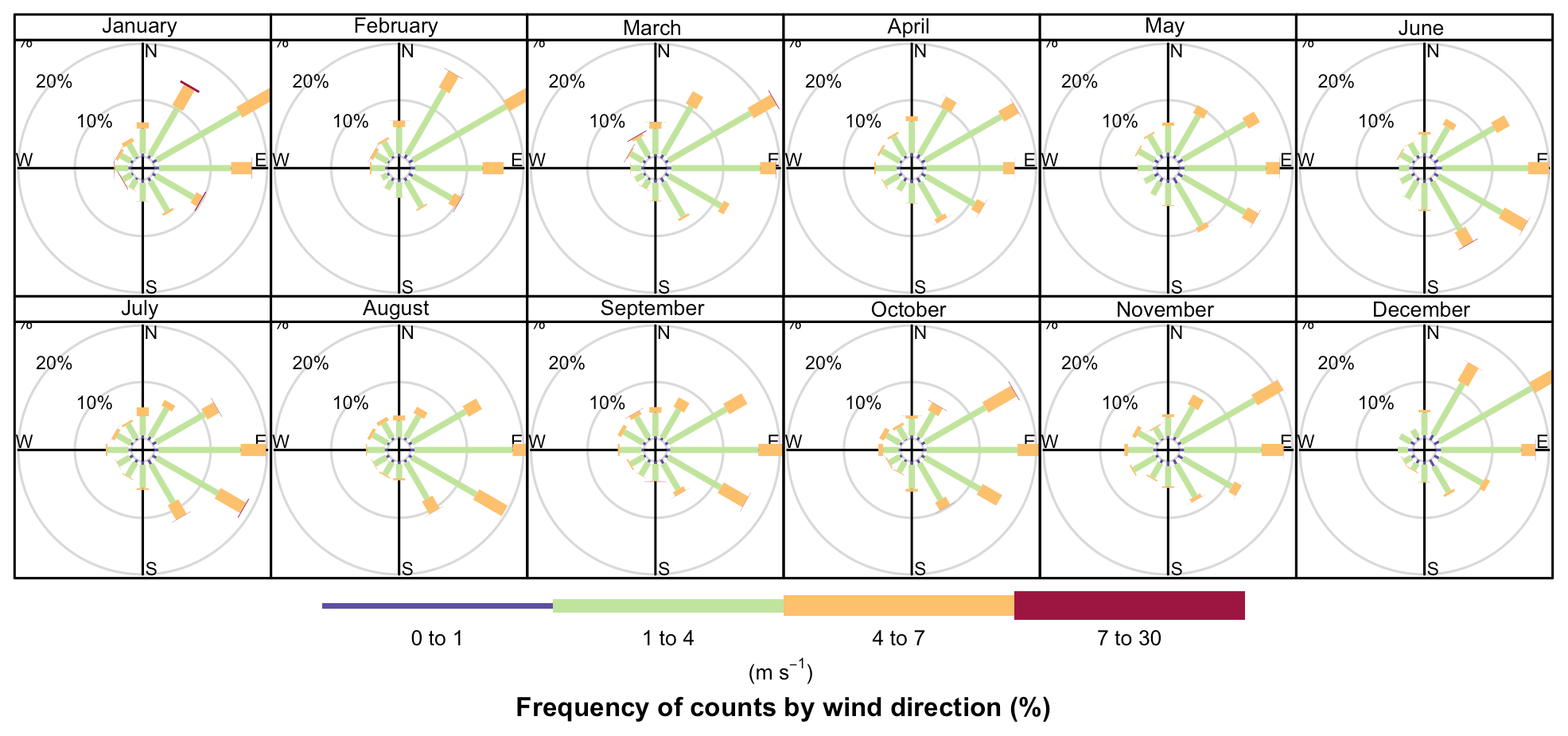
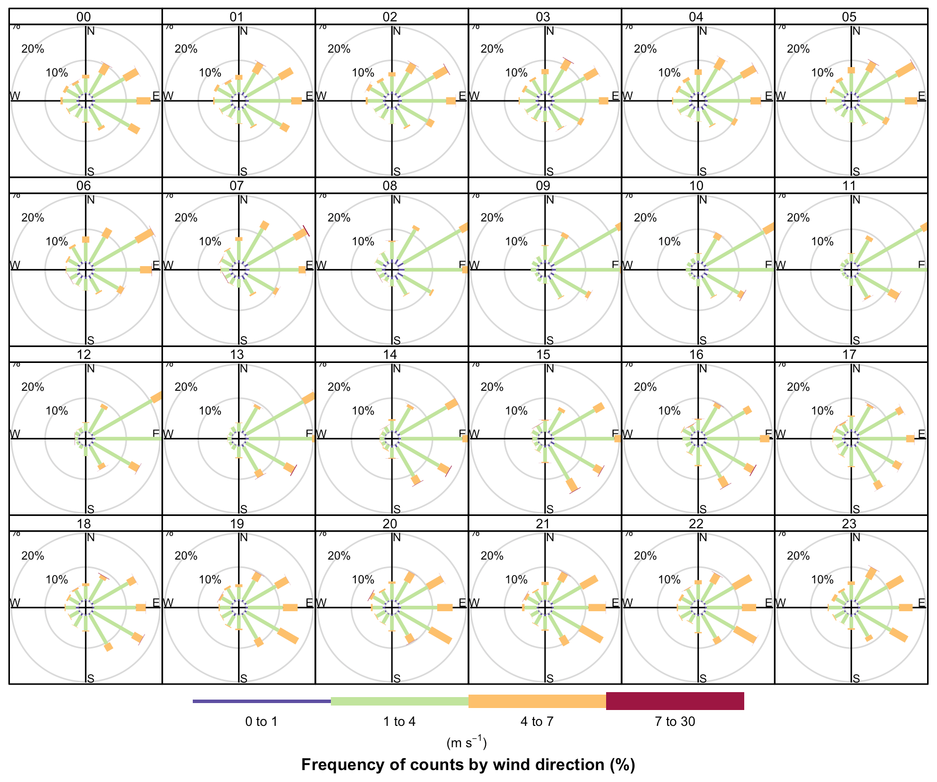
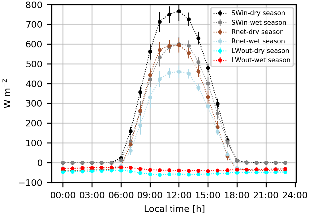
Figure B1 Net, shortwave incoming and longwave outgoing radiation for dry and wet seasons at ATTO.

Appendix C: Dead stands of flooded forest

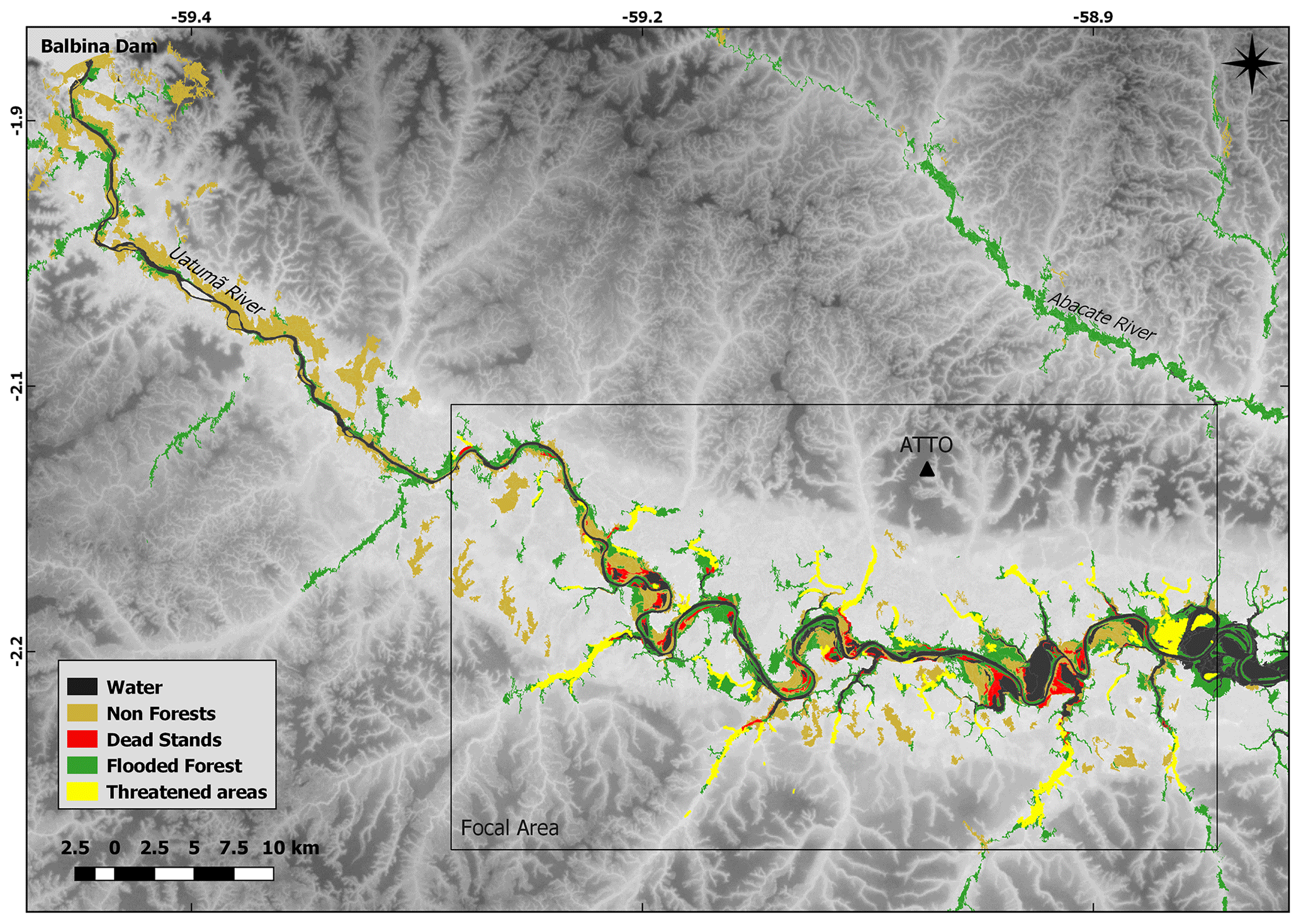
Figure C1 Map showing the dead stands and potentially threatened areas due to the tree mortality caused by the Balbina Dam. This map was modified from Resende et al. (2019), with permission from Elsevier.