the Creative Commons Attribution 4.0 License.
the Creative Commons Attribution 4.0 License.
 | 05 Jun 2020
The isotopic composition of atmospheric nitrous oxide observed at the high-altitude research station Jungfraujoch, Switzerland
Eliza Harris
Stephan Henne
Sarah Eggleston
Martin Steinbacher
Lukas Emmenegger
Christoph Zellweger
Joachim Mohn
Atmospheric nitrous oxide (N2O) levels have been continuously growing since preindustrial times. Mitigation requires information about sources and sinks on the regional and global scales. Isotopic composition of N2O in the atmosphere could contribute valuable constraints. However, isotopic records of N2O in the unpolluted atmosphere remain too scarce for large-scale N2O models. Here, we report the results of discrete air samples collected weekly to biweekly over a 5-year period at the high-altitude research station Jungfraujoch, located in central Switzerland. High-precision N2O isotopic measurements were made using a recently developed preconcentration and laser spectroscopy technique. The measurements of discrete samples were accompanied by in situ continuous measurements of N2O mixing ratios. Our results indicate a pronounced seasonal pattern with minimum N2O mixing ratios in late summer, associated with a maximum in δ15Nbulk and a minimum in intramolecular 15N site preference (δ15NSP). This pattern is most likely due to stratosphere–troposphere exchange (STE), which delivers N2O-depleted but 15N-enriched air from the stratosphere into the troposphere. Variability in δ15NSP induced by changes in STE may be masked by biogeochemical N2O production processes in late summer, which are possibly dominated by a low-δ15NSP pathway of N2O production (denitrification), providing an explanation for the observed seasonality of δ15NSP. Footprint analyses and atmospheric transport simulations of N2O for Jungfraujoch suggest that regional emissions from the planetary boundary layer contribute to seasonal variations of atmospheric N2O isotopic composition at Jungfraujoch, albeit more clearly for δ15NSP and δ18O than for δ15Nbulk. With the time series of 5 years, we obtained a significant interannual trend for δ15Nbulk after deseasonalization ( ‰ a−1), indicating that the atmospheric N2O increase is due to isotopically depleted N2O sources. We estimated the average isotopic signature of anthropogenic N2O sources with a two-box model to be ‰ for δ15Nbulk, 34.8±3 ‰ for δ18O and 10.7±4 ‰ for δ15NSP. Our study demonstrates that seasonal variation of N2O isotopic composition in the background atmosphere is important when determining interannual trends. More frequent, high-precision and interlaboratory-compatible measurements of atmospheric N2O isotopocules, especially for δ15NSP, are needed to better constrain anthropogenic N2O sources and thus the contribution of biogeochemical processes to N2O growth on the global scale.
- Article
(5873 KB) - Full-text XML
-
Supplement
(644 KB) - BibTeX
- EndNote


Nitrous oxide (N2O) is a potent greenhouse gas (Fowler et al., 2015) and a strong stratospheric ozone-depleting substance (Ravishankara et al., 2009). For several decades, near-surface atmospheric N2O mixing ratios have been continuously measured at a series of remote sites, within the networks of the Global Atmosphere Watch program (JMA and WMO, 2018), the Advanced Global Atmospheric Gases Experiment (AGAGE) (Prinn et al., 2018) and the National Oceanic and Atmospheric Administration (NOAA) Earth System Research Laboratory (ESRL) Global Monitoring Division (GMD) (Nevison et al., 2011). These measurements have shown a significant increase in atmospheric N2O mixing ratio, at a current growth rate of about 0.93 nmol mol−1 a−1 (WMO, 2018). On the global scale, given excessive nitrogen (N) fertilizer application, agriculture is known to be the largest and most important anthropogenic source of N2O (Reay et al., 2012; Tian et al., 2019). However, long-term observations of N2O in the unpolluted atmosphere have shown seasonal and interannual variabilities as well as interhemispheric differences in N2O mixing ratios (Nevison et al., 2011; Thompson et al., 2014a, b), which cannot yet be resolved by atmospheric transport models and existing emission inventories. Moreover, regional contributions of N2O emissions and the strengths of individual N2O production pathways remain difficult to quantify.
Isotopic signatures of atmospheric N2O can provide important constraints on N2O sources (Denk et al., 2017) and trends (Kim and Craig, 1993). The ratios of 15N∕14N and 18O∕16O in N2O are often reported in δ notation as δ(15N∕14N) and δ(18O∕16O), abbreviated as δ15Nbulk (average for 14N15N16O and 15N14N16O) and δ18O, respectively. A large fraction of N2O emitted to the atmosphere originates from soil bacterial processes, which usually emit N2O that is more enriched in light (14N, 16O) isotopes than the tropospheric background (Pérez et al., 2001; Snider et al., 2015a; Toyoda et al., 2017). By contrast, N2O produced in the oceans (Bourbonnais et al., 2017; Fujii et al., 2013) and emitted from fossil fuel combustion (Ogawa and Yoshida, 2005; Toyoda et al., 2008) has higher δ15Nbulk and δ18O values which are comparable to the tropospheric background. A recent study has summarized isotopic signatures of anthropogenic N2O sources divided into the EDGAR (Emissions Database for Global Atmospheric Research) emission categories (Janssens-Maenhout et al., 2019), showing differences in isotopic signatures between agricultural (δ15Nbulk = −17.8 ‰ to −1.0 ‰ and δ18O = 23.9 ‰ to 29 ‰) and industrial sources (δ15Nbulk = −28.7 ‰ to 5.5 ‰ and δ18O = 28.6 ‰ to 40.3 ‰) (Harris et al., 2017). These empirical ranges, together with isotopic mixing models, provide a valuable approach to interpret variability in atmospheric N2O mixing ratios.
A number of studies have analyzed temporal trends in N2O isotopic composition in the modern atmosphere (Kaiser et al., 2003; Park et al., 2012; Röckmann and Levin, 2005; Toyoda et al., 2013) and in the past from firn and ice cores (Bernard et al., 2006; Ishijima et al., 2007; Prokopiou et al., 2018; Röckmann et al., 2003; Sowers et al., 2002). These isotopic measurements have shown a decrease in both δ15Nbulk–N2O and δ18O–N2O associated with an increasing trend in atmospheric N2O mixing ratios since preindustrial times, indicating that the recent increase of atmospheric N2O may be due to agricultural emissions (15N and 18O depleted). The reported trend since the 1960s seems rather steady ( ‰ a−1 for δ15Nbulk and −0.016 ± 0.006 ‰ a−1 for δ18O) (Bernard et al., 2006; Ishijima et al., 2007; Park et al., 2012; Prokopiou et al., 2017; Röckmann et al., 2003; Röckmann and Levin, 2005). However, a more recent (1999–2010) study reported a smaller decreasing trend in δ15Nbulk and only an insignificant trend in δ18O for the Northern Hemisphere (Toyoda et al., 2013). Several hypotheses were proposed to explain the differences in the observed trends: (1) the interhemispheric difference in N2O emission sources results in inconsistent isotopic signatures among different studies (Thompson et al., 2014b); (2) uncertainties in isotopic measurements and variable sampling schemes (air type, sampling frequency and time) mask the small secular trend of N2O isotopic composition in the background atmosphere (Toyoda et al., 2013); and/or (3) N2O source isotopic signatures have changed in recent years, possibly due to shifts in N fertilizer type and climatic forcing (Tian et al., 2019). Hence, further investigation into the global N2O source inventory and its evolution over time requires more frequent, precise measurements of N2O isotopocules in the unpolluted atmosphere, particularly in the Northern Hemisphere.
Recently, site-specific compositions of N2O isotopomers (site preference: δ15NSP), which denote the difference of 15N between the central (14N15N16O, α position) and terminal (15N14N16O, β position) N atoms, has been applied to constrain sources contributing to atmospheric N2O (Toyoda et al., 2013; Yoshida and Toyoda, 2000). δ15NSP of N2O is particularly effective for distinguishing between the major N2O production processes, i.e., nitrification and denitrification, generally referred to as aerobic and anaerobic N2O production, with high and low δ15NSP, respectively (Sutka et al., 2006). However, despite the advantages of δ15NSP measurements, existing long-term studies have not yet been able to reach a definitive understanding of the δ15NSP−N2O trend, showing both positive (Bernard et al., 2006; Park et al., 2012; Röckmann and Levin, 2005) and negative tendencies (Röckmann et al., 2003) over the last 4 decades. This is probably due to an insufficient analytical precision and poor interlaboratory agreement, in particular as the aforementioned studies are all based on isotope ratio mass spectrometry (IRMS). To retrieve site-specific isotopic information by IRMS, the N2O+ molecular ions and the NO+ fragment ions are analyzed, and raw data have to be corrected for rearrangements of central and terminal N and 17O content (Toyoda et al., 2001). Inappropriate correction algorithms and the limited availability of reference materials (Ostrom et al., 2018) further enlarge the analytical uncertainty (Mohn et al., 2014).
Seasonal variability in atmospheric N2O isotopic composition, which could affect the longer-term trends, is still rarely reported in the literature (Park et al., 2012; Toyoda et al., 2013). Moreover, studies of seasonality of N2O isotopic composition are limited to the recent past since the air samples derived from firn and ice cores suffer from coarse temporal resolution (<2 samples per year). Park et al. (2012) studied seasonality of atmospheric N2O isotopic composition by analyzing a set of archived air samples collected from Cape Grim (Australia) using a sophisticated mathematical modeling approach. They found consistent seasonal patterns in δ15Nbulk, δ18O and δ15NSP of atmospheric N2O, showing highest 15N∕18O enrichment in June and lowest in December. This pattern was negatively correlated with the seasonality of the N2O mixing ratios (lowest in April–May and highest in December), which is in agreement with a previous study by Nevison et al. (2011). The negative correlation between isotopic composition and mixing ratios has been explained by stratosphere–troposphere exchange (STE), which transports N2O-depleted but isotopically enriched stratospheric air (prevailing reduction process) into the lower atmosphere (Yung and Miller, 1997). However, in a more recent study from Hateruma Island (Japan), Toyoda et al. (2013) reported insignificant seasonal patterns in atmospheric N2O isotopocules (smaller variability than measurement precision), despite their finding of a somewhat similar seasonal pattern in N2O mixing ratio (minimum in July). Although there are interhemispheric differences in N2O sources and distinct sampling frequencies in the two studies discussed above (2–3 times per year versus monthly), it is noteworthy that both studies observed significantly larger variability in δ15NSP than in δ15Nbulk and δ18O. Whether the fluctuations in δ15NSP are mainly caused by the limited repeatability of the chosen analytical techniques or interplay of processes or mechanisms regulating atmospheric N2O remains to be tested (Park et al., 2012).
With inherent selectiveness, in particular for site-specific isotopic composition, laser spectroscopy provides a new analytical approach for direct, precise measurements of all four N2O isotopocules (Harris et al., 2014; Mohn et al., 2012). The recent development of quantum cascade laser absorption spectroscopy (QCLAS) coupled with an automated preconcentration unit has been applied to measure N2O isotopocules in ambient air, with comparable precision for δ15Nbulk and δ18O and superior precision for δ15NSP relative to IRMS systems (Harris et al., 2017; Mohn et al., 2014). Here, we present results from the application of a preconcentration unit coupled to QCLAS to measure atmospheric N2O isotopocules in background air collected at the high-altitude research station Jungfraujoch, Switzerland. Between April 2014 and December 2018, we collected weekly to biweekly air samples for N2O isotopic analyses, in parallel with online measurement of N2O mixing ratios. To our knowledge, this work reports the first time series of background atmospheric N2O isotopic composition using laser spectroscopy. With this unique dataset, we aim to (1) constrain seasonal patterns of three N2O isotopic signatures at the Jungfraujoch observatory; (2) determine interannual trends in N2O isotopocules, especially δ15NSP; and (3) interpret the observed patterns in N2O mixing ratios using temporal trends in N2O isotopic composition and reported isotopic signatures of anthropogenic sources.
2.1 Site description
The high-altitude research station Jungfraujoch (3580 m a.s.l.), located on the northern ridge of the Swiss Alps, is a well-established site for studying unpolluted atmosphere over central Europe (e.g., Buchmann et al., 2016). Although the station is located in the free troposphere most of the time, it is occasionally affected by air recently lifted from the planetary boundary layer (Herrmann et al., 2015; Zellweger et al., 2003). Henne et al. (2010) investigated the representativeness of 35 European monitoring stations and categorized Jungfraujoch as “mostly remote”. The Jungfraujoch station is part of several national and international networks, like the meteorological SwissMetNet operated by MeteoSwiss, the Swiss National Air Pollution Monitoring Network (NABEL), the Global Atmospheric Watch program (GAW) of the World Meteorological Organization (WMO) and the Integrated Carbon Observation System (ICOS) Research Infrastructure. This results in an extended set of long-term and continuously available parameters such as meteorological variables (Appenzeller et al., 2008); greenhouse gases (Schibig et al., 2015; Sepúlveda et al., 2014; Yuan et al., 2018); CO2 isotopic composition (Sturm et al., 2013; Tuzson et al., 2011); ozone-depleting substances; and their replacement products (Reimann et al., 2008), atmospheric pollutants (Logan et al., 2012; Pandey Deolal et al., 2012; Zellweger et al., 2009), and aerosol parameters (Bukowiecki et al., 2016).
2.2 In situ measurements and discrete air sampling (flasks)
In situ observations of N2O mixing ratios commenced at Jungfraujoch in December 2004. Initially, measurements were made with a gas chromatograph (GC) (Agilent 6890N, USA) followed by electron capture detection (ECD). The time resolution of these measurements was 24 to 30 min. In late 2014, we implemented a cavity-enhanced off-axis integrated cavity output spectroscopy analyzer (OA-ICOS, Los Gatos Research Inc., Mountain View, CA, USA), which measures the atmospheric N2O mixing ratio continuously. Measurements of N2O mixing ratios at Jungfraujoch were calibrated with three standard gases (319, 327 and 342 nmol mol−1) and accompanied with measurement of a working standard (331 nmol mol−1) every 160 min to account for instrumental drift. In addition, short- (two times every 40 h) and long-term (every 40 h) target measurements were included to monitor the data quality. Due to the superior measurement precision compared to the GC-ECD method (Lebegue et al., 2016), the OA-ICOS record has become the primary time series since January 2015. The GC-ECD observations continued until summer 2016 for comparison and quality control.
Additional parameters, recorded within NABEL and the ICOS infrastructure, were included in the analysis below. These data were carbon monoxide (CO) (measured by cavity ring-down spectroscopy; model G2401, Picarro Inc., USA), the sum of oxidized nitrogen species (NOy) (measured by chemiluminescence detection after conversion of NOy to NO on a heated gold catalyst; CLD 89p, Eco Physics, Switzerland) and O3 (measured by UV absorption; TEI 49i, Thermo Scientific, USA). Details on measurement methods and calibration strategies can be found in Zellweger et al. (2009) for CO, Pandey Deolal et al. (2012) for NOy and Logan et al. (2012) for O3.
In conjunction with the online measurements, we deployed an automated sampling system (Fig. S1 in the Supplement) to collect pressurized air samples in aluminum cylinders from the same air inlet at the Sphinx Observatory of the Jungfraujoch station for subsequent N2O mixing ratio and isotopic analyses. The sample collection was conducted weekly from April 2014 to February 2016. After a sampling gap of 5 months due to a technical failure, we reinitiated a biweekly sampling, which continued from August 2016 to December 2018. The sampling system, automated by a customized LabVIEW program (National Instruments Corp., USA), consisted of a Nafion drier (PD-100T-48MSS, Perma Pure LLC, USA), a membrane gas compressor (KNF Neuberger, USA; type N286 series), a 16-port selector valve (EMT2CSD16MWEPH, VICI AG, Switzerland), and a rack to accommodate nine 2 L aluminum flasks (Luxfer, Messer Schweiz AG, Switzerland). During sample filling, pre-evacuated flasks were first purged with ambient air five times (1 h) and then filled to 12 000 hPa within 40 min, resulting in approximately 24 L (298 K and 1000 hPa) of air per flask for isotopic analysis. Air sample filling generally took place between 14:00 and 15:00 LT (local time) at each sampling day. Sample flasks were sent back to the laboratory at Empa for analyses every few months. For this study, 142 air samples were collected in flasks and analyzed for N2O isotopocules.
2.3 Analyses of discrete air samples
Discrete air samples were regularly analyzed in batches but not in chronological order to prevent the imprint of analytical drifts on temporal trends of the samples. N2O mole fractions were analyzed by QCLAS (CW-QC-TILDAS-76-CS, Aerodyne Research Inc., USA) against NOAA standards on the WMO-X2006A calibration scale (Hall et al., 2007), at a precision around 0.1 nmol mol−1 (determined with the average of 1 min data).
The four most abundant N2O isotopocules (14N14N16O, 99.03 %; 14N15N16O, 0.36 %; 15N14N16O, 0.36 %; 14N14N18O, 0.20 %) were analyzed using a customized QCLAS system (Aerodyne Research, Inc., USA) (Heil et al., 2014) coupled with an automated preconcentration device (Mohn et al., 2010). Before entering the preconcentration unit, sample air is passed through a Sofnocat 423 trap (Molecular Products Limited, GB) to remove CO and subsequently through an Ascarite trap (Ascarite: 6 g, 10–35 mesh, Sigma Aldrich, Switzerland, bracketed by Mg(ClO4)2, 2×1.5 g, Alfa Aesar, Germany) to remove CO2 and water. Approximately 5.5 L of air with a flow of 250 mL min−1 (at 295 K and 3500 hPa) is then passed through a HayeSep D trap cooled to −145 ∘C to collect N2O (Mohn et al., 2010). For N2O release to the multipath cell of the QCLAS, the HayeSep D trap is quickly heated to 10 ∘C and flushed with high-purity synthetic air (20.5 % of O2 in N2) carrier gas at a flow rate of 25 mL min−1 (at 295 K and 3500 hPa). A final cell pressure around 16 hPa is achieved, which results in an N2O mixing ratio of about 45 µmol mol−1. More instrumental details can be found in previous studies (Harris et al., 2017; Mohn et al., 2010, 2012). Sample tanks were each analyzed twice to yield duplicates for N2O isotopic results, which left sufficient air for amount fraction analysis as described in the previous paragraph.
2.4 Data analyses
We used 10 min averages of the continuous in situ measurements from the Jungfraujoch station across this study. For a point-to-point comparison of continuous and discrete measurements of N2O mixing ratio, we aggregated 10 min averages of in situ data for the same period when the discrete sample was filled into the cylinder (40 min).
In this study, we report abundances of N2O isotopocules using δ notation (‰) as below:
where X refers to 15Nα (14N15N16O), 15Nβ (15N14N16O) and 18O (14N14N18O); R refers to the ratio between the amount fractions of the rare isotopocules as mentioned above and the amount fraction of 14N14N16O; isotope standards refer to atmospheric N2 for 15N and Vienna Standard Mean Ocean Water (VSMOW) for 18O.
Hence, the total 15N content of N2O and site-specific composition of N2O isotopomers could be further illustrated as δ15Nbulk and δ15NSP, respectively, according to the equations below:
Two standards (CG1 and CG2; in 79.5 % N2 and 20.5 % O2) with distinct isotopic signatures (δ15Nα = 16.29±0.07 ‰ (CG1) and ‰ (CG2); δ15Nβ = ‰ and ‰; δ18O = 39.37±0.04 ‰ and 30.81±0.03 ‰) were used for calibrating isotopic composition. The calibration gases CG1 and CG2 were calibrated on the Tokyo Institute of Technology (TIT) scale, based on cross-calibration with primary standards assigned by TIT (Mohn et al., 2012, 2014). In addition, CG1 was measured repeatedly between samples and target gases to account for instrumental drift. Both CG1 and CG2 have N2O mixing ratios of 45 µmol mol−1, similar to the N2O amount fraction of the samples after preconcentration. However, to correct for possible instrumental dependence on N2O mixing ratio, CG1 was diluted to N2O mole fractions of 35–40 µmol mol−1 within each measurement batch. In general, duplicated isotopic measurements of flask samples yielded values of repeatability of 0.10 ‰–0.20 ‰ for δ15Nbulk and δ18O and 0.15 ‰–0.25 ‰ for δ15NSP.
At the beginning of the project, a batch of three cylinders (50 L water volume, Luxfer, Italy) were filled with pressurized ambient air in Dübendorf with an oil-free three-stage compressor (SA-3, Rix Industries, USA) and used as long-term target gases. The pressurized ambient air target gas was analyzed with identical treatment as Jungfraujoch air samples during every analysis batch to monitor long-term analytical drift. Standard deviations for repeated target gas measurements throughout the period of Jungfraujoch sample measurements were 0.13 ‰ for δ15Nbulk, 0.21 ‰ for δ15NSP and 0.11 ‰ for δ18O (Fig. S2).
2.5 Surface air footprint analysis and simulated regional N2O enhancement
We analyzed the air mass origin at Jungfraujoch by applying the Lagrangian particle dispersion model (LPDM) FLEXPART (FLEXible PARTicle dispersion model) in the backward mode (Stohl et al., 2005). The model was driven by meteorological fields taken from the ECMWF-IFS operational analysis cycle, extracted at a resolution of , 90∕137 levels globally and at higher horizontal resolution of for central Europe. We released 50 000 virtual air parcels every 3 h at 3000 m a.s.l. from Jungfraujoch to perform backward dispersion simulations over 10 d, which allowed us to calculate surface source sensitivities (concentration footprints). A release height of 3000 m a.s.l. was previously determined to be an optimum for simulating concentration footprints at Jungfraujoch, given the stated horizontal resolution which results in a considerable smoothing of the complex, alpine orography (Keller et al., 2012). The 3-hourly surface footprints for the whole observation period were used to categorize different transport regimes using the clustering approach outlined in Sturm et al. (2013). This allowed us to distinguish among six different source regions: Free Troposphere (FT), Southwest (SW), East (E), Local (L), West (W) and Northwest (NW).
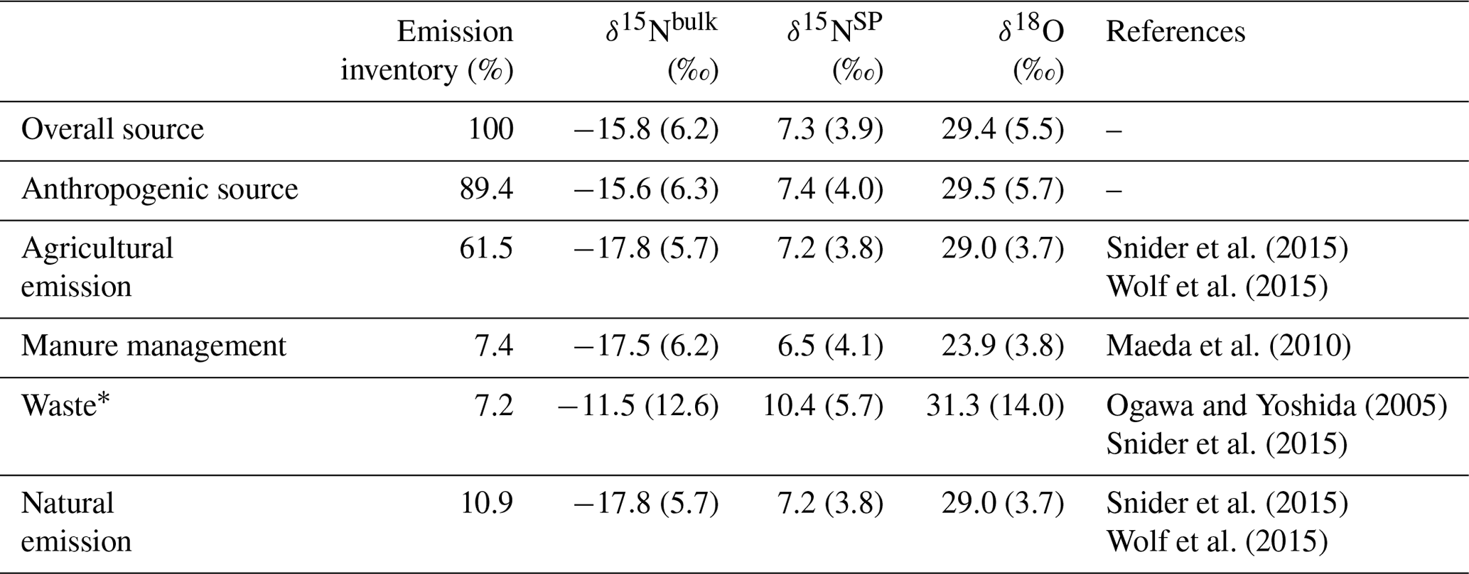
Table 1An overview of N2O emission sectors for the Swiss Meteotest inventory and the global EDAGR inventory and available source isotopic signatures (‰)1.
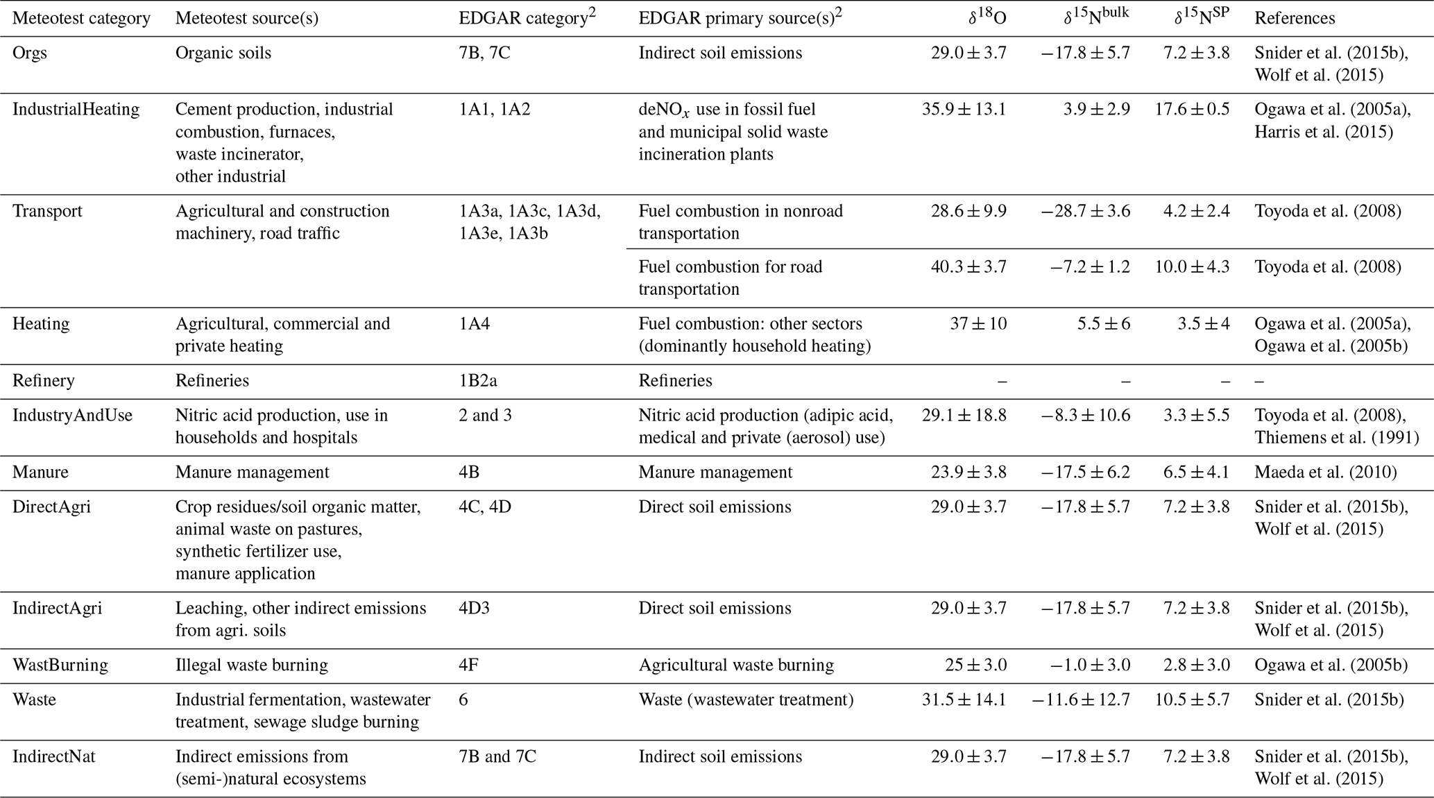
1 Isotopic signatures for anthropogenic sources are obtained from the summary by Harris et al. (2017). 2 These are the primary sources contributing to N2O emissions in Switzerland.
Similar to Henne et al. (2016) for CH4 and based on spatially resolved N2O emission inventories (Meteotest for Switzerland; EDGAR for Europe), we used the FLEXPART concentration footprints to calculate time series of atmospheric mole fraction increases at Jungfraujoch resolved by emission sectors (Henne et al., 2016). The emission inventory by Meteotest consists of 12 emission sectors, among which all sectors except “organic soils” are comparable to sectors in the EDGAR inventory (See Table 1) (Janssens-Maenhout et al., 2019). To improve seasonal representation of the emissions in our model, we used a monthly resolved optimized version of the emission inventory, which was obtained through inverse modeling using the N2O atmospheric mole fractions observed between March 2017 and September 2018 at the tall tower site Beromünster on the Swiss plateau (Henne et al., 2019). Therefore, in this study, source contributions to Jungfraujoch were estimated specifically for the period mentioned above.
2.6 Evaluation of seasonal pattern and interannual trend for time series
To explore seasonality and interannual trends, we fit the time series of in situ measurements of N2O and O3 mixing ratios, NOy-to-CO ratios and isotopic measurements of N2O with polynomial functions and Fourier series (four harmonics for in situ measurements and two harmonics for discrete measurements) (Thoning et al., 1989). Time series were then decomposed into a linear trend, seasonal variability (per 12 months) and residuals. This fit was conducted with a nonlinear least-squares (NLS) model with R version 3.5.3 (R Core Team, 2016). The detrended seasonality was examined by comparing peak-to-peak amplitudes with our analytical precisions and the uncertainty given by the 1 standard deviation of monthly residuals. To determine interannual trends, a linear regression was applied to both the raw and the deseasonalized datasets. The significance level is set to p<0.01. The interannual trends for N2O mixing ratios were found to be little affected by seasonality, so growth rates were determined only based on the raw datasets.
Although Jungfraujoch is a remote site, episodic influence from the planetary boundary layer can be observed at the station (Pandey Deolal et al., 2012; Zellweger et al., 2003). For evaluating trends of N2O mixing ratio measurements, we filtered out in situ data with significant influence from the plenary boundary layer in order to represent a major air mass footprint from the free troposphere (FT). In addition to the air transport regimes, an alternative filtering criterion for the free troposphere was based on the published mean ranges of NOy mixing ratios (501–748 pmol mol−1 depending on the season) and NOy-to-CO ratios (0.003–0.005 depending on the season) at Jungfraujoch (Zellweger et al., 2003). This criterion is less strict than that given by footprint analyses (Herrmann et al., 2015). After applying this criterion to the isotopic time series (which led to the exclusion of 32 measurement points), we reevaluated the seasonal and interannual trends in the N2O isotopic composition. In addition, because of the strong variability observed for isotopic data during the first 1.5 years (until February 2016), we performed an independent evaluation for the time series starting from August 2016.
2.7 Two-box model simulation
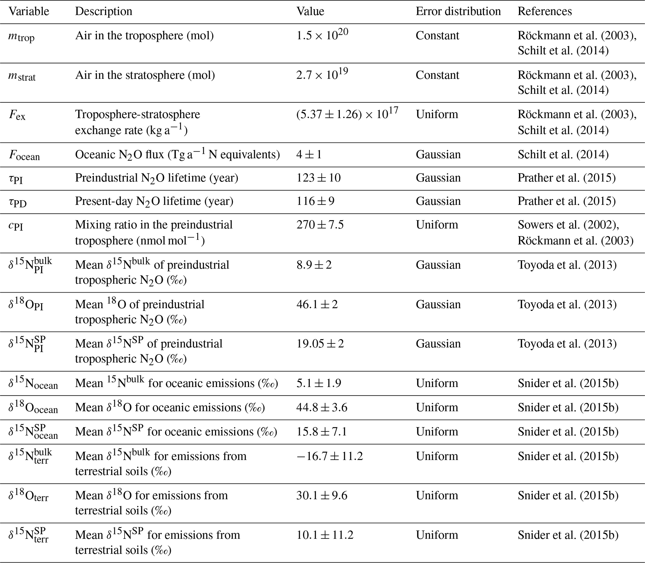
A two-box model representing a well-mixed troposphere and stratosphere was used to estimate the anthropogenic N2O source strength and isotopic composition from the trends measured at Jungfraujoch, similar to the approaches used by several previous studies (Ishijima et al., 2007; Röckmann et al., 2003; Schilt et al., 2014; Sowers et al., 2002). The input variables used to run the model are given in Table 2. The 200 iterations of the model were run using a Monte Carlo-style approach to approximate the uncertainty considering the uncertainty distribution for each input variable as given in Table 2. All variables were set independently within the Monte Carlo approximation except for preindustrial N2O lifetime (τPI), which was fixed to 106 % of the present-day N2O lifetime τPD (Prather et al., 2015).
Within each iteration of the model, the preindustrial N2O burden was first described, assuming steady state in the preindustrial era. The preindustrial stratospheric N2O mixing ratio (cS,PI) (270±7.5 nmol mol−1) was taken from Sowers et al. (2002):
where Fex refers to the troposphere–stratosphere exchange rate, cPI refers to the preindustrial tropospheric N2O mixing ratio, and MPI and MS,PI are the masses of N2O in the troposphere and stratosphere, respectively. The preindustrial terrestrial flux in Sowers et al. (2002) (Eq. 2) was used here assuming no anthropogenic emissions. The delta values for the preindustrial stratosphere and the fractionation factor for the stratospheric sink were taken from Eqs. (6) and (7) from Sowers et al. (2002), assuming steady state and no anthropogenic emissions. The model was run with a yearly time step starting from the preindustrial period, assuming that anthropogenic emissions began in 1845 (Sowers et al., 2002). For each year of the model run, the anthropogenic flux was calculated according to the exponential increase described by Sowers et al. (2002):
where t is the current year, t0=1845 and α is the growth rate (assumed to be constant). The rates of change for tropospheric and stratospheric N2O mixing ratios were then retrieved from Eqs. (2) and (3) in Sowers et al. (2002) and for the isotopic composition of stratospheric and tropospheric N2O from Eqs. (6) and (7) in Sowers et al. (2002).
The values of the parameters describing the anthropogenic flux were optimized to fit both the trend and the absolute values for the 5 years of Jungfraujoch isotope data and the mixing ratio data from the Jungfraujoch flasks and in situ data since 2005 (GAW data source). The uncertainties in α and in the anthropogenic source isotopic signatures were approximated by 1 standard deviation of values derived from repeated model runs.
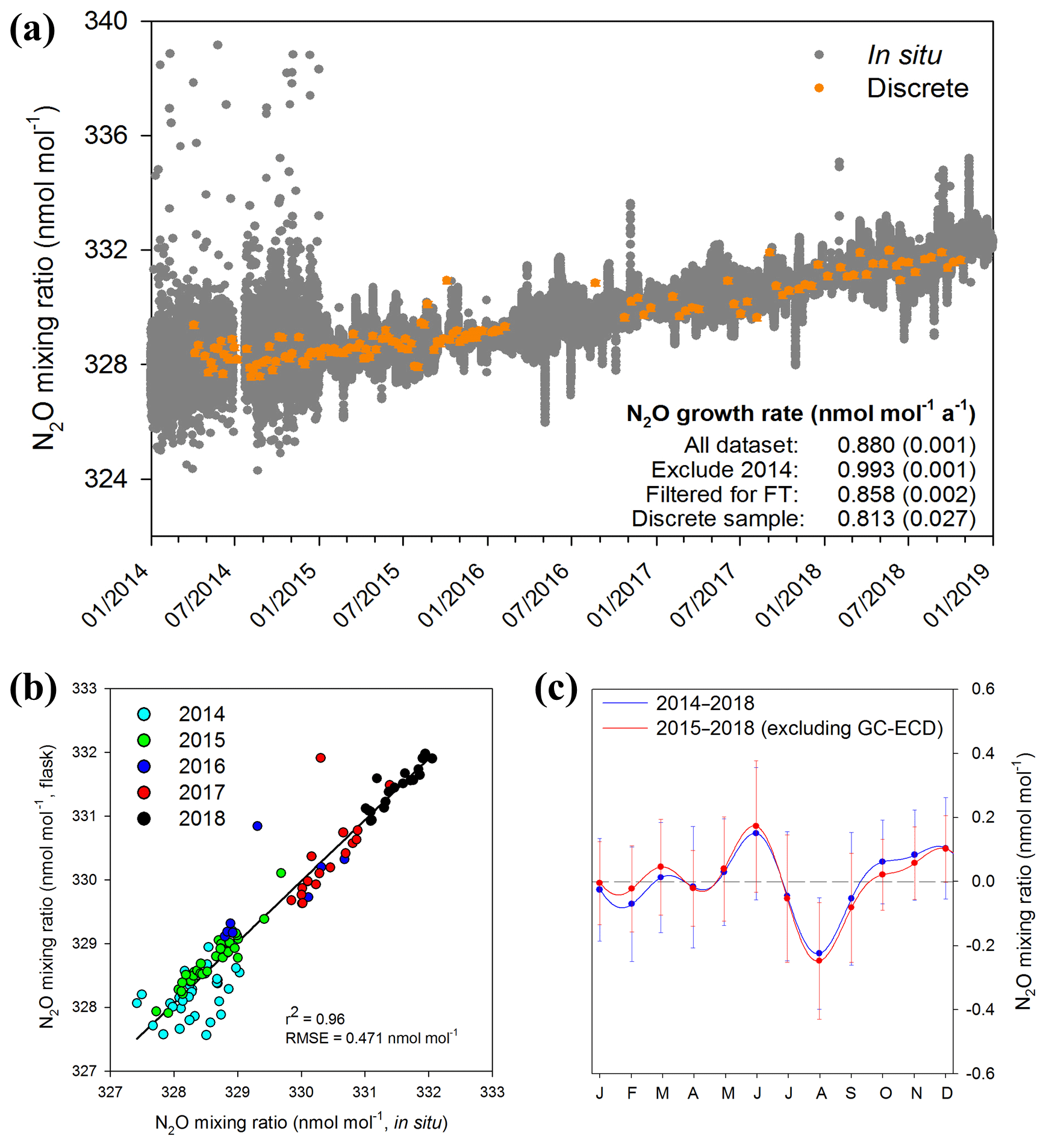
Figure 1(a) In situ (10 min averages) and discrete measurements of N2O mixing ratios from April 2014 to December 2018 at Jungfraujoch. In situ N2O mixing ratio measurements were performed with the GC-ECD method between April and December 2014. After that, OA-ICOS became the major analytical method for in situ measurements. Discrete sample points are presented as averages with error bars (1 standard deviation). Annual N2O growth rates determined by linear regression are given in the figure (uncertainty shown as 1 standard deviation). A sampling gap exists for discrete samples between February and August 2016. (b) Comparison of in situ and discrete measurements of N2O mixing ratios; in situ measurements were 10 min values averaged over the exact period of discrete sampling time (∼40 min); in situ measurements were performed with the GC-ECD method in 2014, and this was replaced with the OA-ICOS method from January 2015. (c) Seasonality of N2O mixing ratios at Jungfraujoch derived from in situ measurements. Datasets with and without GC-ECD measurements are compared for seasonality evaluation. The NLS model simulation for time series gives the detrended seasonality, with error bars indicating 1 standard deviation of monthly residuals.
2.8 Evaluation of the combined effects from STE and soil emission on δ15NSP
To evaluate the combined effects of STE and soil emission on the seasonal variability of δ15NSP (i.e., August minima), we made a mixing calculation as given below:
-
For soil emission, when based on the determined seasonality of N2O mole fraction at Jungfraujoch, the maximum N2O mole fraction enhancement was approximately 0.2 nmol mol−1 above baseline (Fig. 1). Hence, we assumed N2O enhancement from soil emission to be close to 0.15 to 0.20 nmol mol−1, which is close to the maximum N2O enhancement in our observation. The isotopic effect from soil emission can be derived from the difference between soil emission (7.2 ‰; Table 1) and tropospheric air (18 ‰, Fig. 2) in δ15NSP, i.e., −10.8 ‰.
-
For mixing with stratospheric air, the minimum of N2O mole fraction in August (−0.20 nmol mol−1) is likely to be the result of both N2O mole fraction enhancement from soil emission and N2O mole fraction depletion due to STE. Given the assumed N2O enhancement from soil emission, we estimated the N2O depletion due to STE as −0.35 to −0.40 nmol mol−1. The isotopic effect due to mixing with stratospheric air can be approximated using the apparent isotopic fractionation εapp (Kaiser et al., 2006), which was derived from the slope of Rayleigh plot with normalized N2O mole and isotope ratios. For 15NSP, εapp is calculated from the difference between 15N∕14N isotope fractionations at the central and terminal N atoms, i.e., αεapp−βεapp. Therefore, for the lower stratosphere, εapp (15NSP) was calculated to be about −15 ‰ (see more details in Kaiser et al., 2006).
-
For the overall effect, when combing the isotope effects and contributions to the change of N2O mole fraction by the two processes, the net effect is ((−0.35 to −0.40 nmol mol−1) (−15 ‰) + (0.15 to 0.20 nmol mol−1) (−10.8 ‰)) ∕ 330 nmol mol−1 ≈0.01 ‰. Such an isotope effect is below our analytical precision and too small to be measured in the background atmosphere.
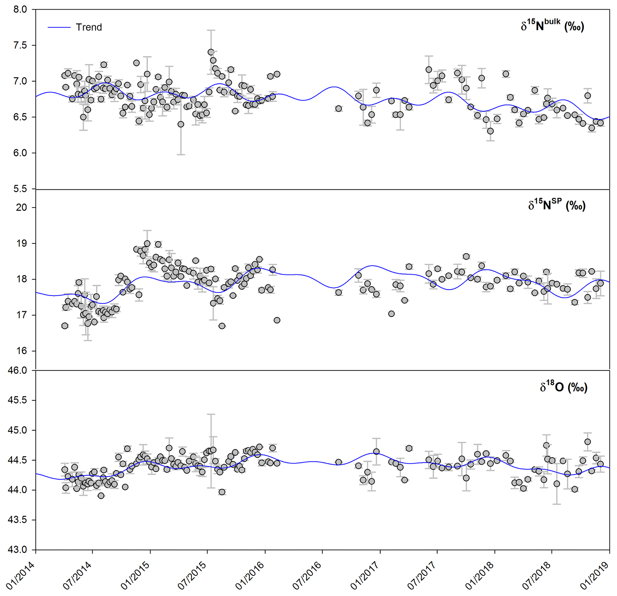
Figure 2Time series of isotopic composition of atmospheric N2O observed at Jungfraujoch from April 2014 to December 2018. Error bars indicate 1 standard deviation of repeated measurements. Blue lines indicate the simulated trends by the NLS model.
2.9 Bottom-up estimates of source isotopic signatures
To gauge the accuracy of the two-box model, we deployed a bottom-up approach as an alternative method of estimating the N2O source signatures. The isotopic signatures of most N2O source sectors given in the Meteotest/EDGAR emission inventory are available from the literature, except for the “Refinery” (Table 1). As “Refinery” generally contributes only about 0.02 % of the N2O emission at Jungfraujoch, it was excluded for source isotopic signature estimation. The simulated N2O emissions by variable sources were categorized according to the EDGAR emission types (Janssens-Maenhout et al., 2019). We then calculated isotopic signatures for the overall source and the anthropogenic sources alone (excluding indirect natural emission) as weighted averages.
3.1 Atmospheric N2O mixing ratios at Jungfraujoch
We observed a linear growth of atmospheric N2O at Jungfraujoch during the period 2014–2018 (Fig. 1a). A point-to-point comparison of discrete and in situ measurements showed good agreement, in particular after the first year (2015–2018), when the data quality of in situ measurements was largely improved due to the implementation of the more precise laser spectroscopy method as compared to GC-ECD (Fig. 1b). The improvement in analytical precision for N2O mixing ratio was due to better temporal coverage by the OA-ICOS instrument in contrast to the GC analyses which conduct one measurement per 24–30 min. The annual growth rates from 2014 to 2018 determined with in situ measurements were 0.880±0.001 and 0.993±0.001 nmol mol−1 a−1 with and without GC-ECD measurements in 2014, respectively. This difference in N2O growth rates is probably due to the limited data quality of GC-ECD, although a lower growth rate in 2014 compared to 2015–2018 cannot be excluded. It is noteworthy that the N2O growth rate determined for 2015 to 2019 at Jungfraujoch is slightly above the global mean growth rate for the recent decade reported by NOAA (0.93±0.03 nmol mol−1 a−1) (WMO, 2018). If we filter the in situ dataset to examine only the “free troposphere” periods, we obtain a lower increase (0.858±0.002 nmol mol−1 a−1). By comparison, the absolute growth rate determined from the discrete gas samples was even lower albeit with larger uncertainty (0.813±0.027 nmol mol−1 a−1).
A significant seasonal pattern was observed for N2O mixing ratios measured in situ, with a maximum in early summer and a minimum in late summer (Fig. 1c). For discrete N2O measurements, a similar trend was observed, but the detrended seasonality was not significant (Fig. S3), which might be due to the much lower number of samples.
3.2 Interannual trends of N2O isotopic composition and anthropogenic source signatures
Time series of δ15Nbulk, δ15NSP and δ18O for atmospheric N2O at Jungfraujoch are shown in Fig. 2. The NLS model simulation accounts well for the variabilities of isotopic time series. Interannual trends of three isotopic deltas were determined for both raw and deseasonalized datasets by linear regression (Table 3). The deseasonalized interannual trends were slightly smaller than the trends determined with the raw datasets. For the whole dataset, the deseasonalized trend indicates a significant decrease in δ15Nbulk of ‰ a−1. In contrast, deseasonalized time series of δ15NSP and δ18O increased, albeit insignificantly, by 0.065±0.027 ‰ a−1 and 0.019±0.011 ‰ a−1, respectively. The trends determined for periods with major air mass footprints from the free troposphere were close to those calculated for the whole dataset, except that δ15NSP trends decreased after filtering out the samples with significant impact from the plenary boundary layer. This indicates that N2O interannual trends observed at Jungfraujoch are of regional relevance, despite the fact that a small impact from local sources can be seen. Because of the observed irregular variability and the change in sampling frequency (though no change in daily sampling time) in our dataset, we separated the time series into two phases: April 2014–February 2016 (first phase; weekly sampling) and August 2016–December 2018 (second phase; biweekly sampling). In the first phase, the rates of increase in δ15NSP and δ18O were almost 1 order of magnitude larger than over the whole dataset. This is most likely due to the unexpectedly low δ15NSP and δ18O in summer 2014 followed by a distinct increase in winter 2014–2015, which results in large rates of increase over short periods. Such growth rates were not seen in the second phase, when both δ15NSP and δ18O showed small and insignificant variations. δ15Nbulk displayed a decreasing interannual trend in both phases; however, the rate of decrease was larger in the second phase ( ‰ a−1).
Table 3Trends of atmospheric δ15Nbulk, δ15NSP and δ18O at Jungfraujoch determined using discrete measurements between April 2014 and December 2018. The trends are determined for the whole dataset, the dataset filtered for free troposphere (removing data points with significant influence from the plenary boundary layer) and the second-phase dataset with biweekly measurements (August 2016 to December 2018).
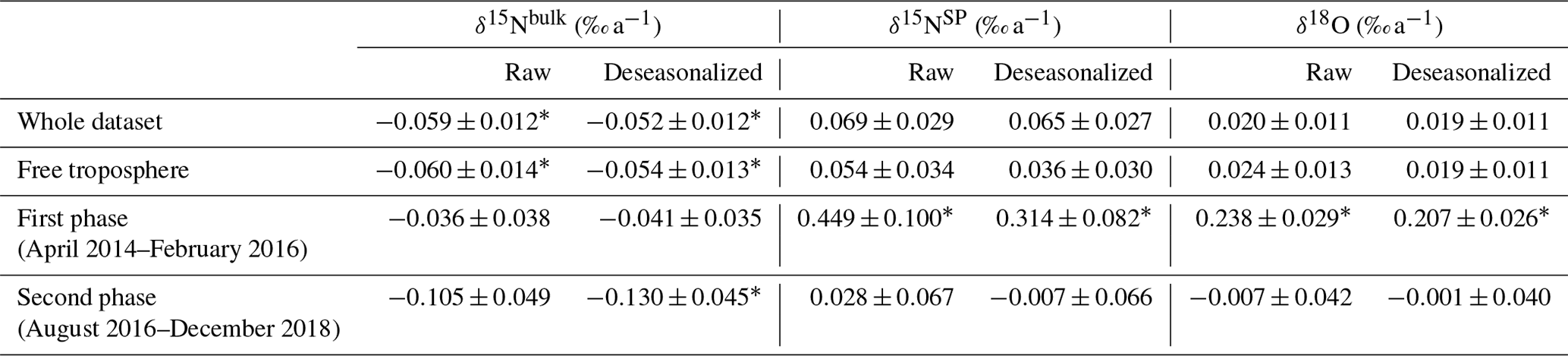
∗ Indicates significance of linear regression.
Table 4Results of the two-box model simulations and selected literature values for comparison.
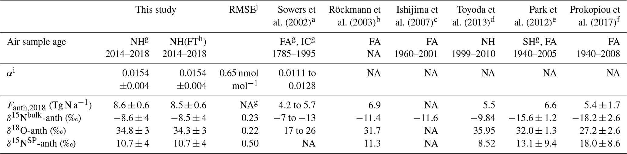
a Estimates are for 1995. b Estimates are for 1998; isotopic signatures of anthropogenic sources were calculated assuming modern tropospheric values to be the same as this study. c Estimate is for 2000; for δ18O, the calibration is not comparable. d Estimates are for 2012 using the “Base” scenario. e Estimates are for 2005. f δanth values are averaged values for the period of 1940–2008. g NH and SH: surface atmosphere from the Northern Hemisphere and Southern Hemisphere, respectively; FA: firn air; IC: ice core air; NA: not available. h FT: Jungfraujoch dataset filtered for free troposphere (based on NOy:CO). i “Value” is the dimensionless constant α describing the exponential increase in the anthropogenic flux. j RMSE refers to root-mean-square error. It is in units of nanomole per mole (nmol mol−1) for α, referring to the present-day tropospheric mixing ratio for N2O. For source isotopic values, RMSE is in the unit of per mill (‰). Simulations with the whole dataset and the dataset filtered for free troposphere yielded the same RMSE.
We tuned our two-box model to best match the observed N2O mixing ratios and isotopic composition at Jungfraujoch. An estimate of anthropogenic emissions and source signatures is given in Table 4. For 2018, annual N2O emissions were estimated to be 8.6±0.6 Tg N2O-N a−1 equivalents. The average isotopic signatures for anthropogenic sources were ‰, 34.8±3 ‰ and 10.7±4 ‰ for δ15Nbulk, δ15NSP and δ18O, respectively, which are clearly lower than those for preindustrial N2O in the tropospheric background (Table 2; Toyoda et al., 2013).
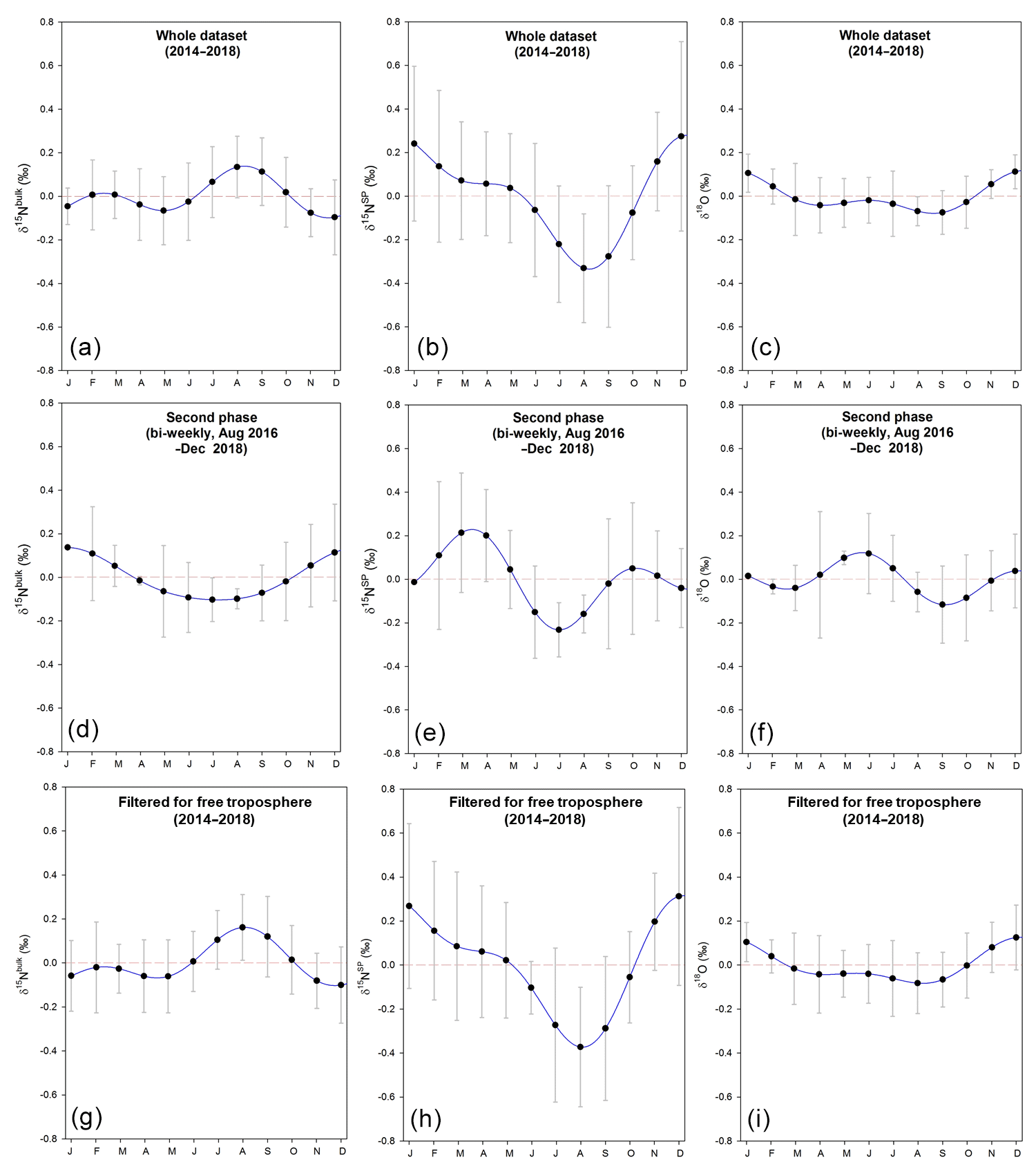
Figure 3Seasonality of isotopic signatures of atmospheric N2O observed at Jungfraujoch. (a–c) Seasonality obtained using the whole dataset from April 2014 to December 2018; (d–f) seasonality obtained using bi-weekly data collected between August 2016 and December 2018; (g–i) seasonality obtained using dataset filtered for free troposphere from April 2014 to December 2018. Dashed red lines refer to zero variability. The NLS model simulation for time series gives the detrended seasonality, with error bars indicating 1 standard deviation of monthly residuals.
3.3 Seasonal variation of N2O isotopic composition
δ15NSP of N2O showed the most pronounced variability among all isotopic time series (Fig. 2), spanning 2.5 ‰ for individual flask sample measurements. Seasonal variability was estimated with the NLS model and presented as mean seasonal cycles (Fig. 3). For δ15NSP, a “summer minimum” was found regardless of whether the entire dataset or only the second phase was considered (Fig. 3); although, seasonal variability of the second time series was smaller and showed the minimum occurring earlier. The seasonal pattern of δ15Nbulk determined from the whole dataset indicates a significant summer maximum, but this was not seen when only the data from the second phase was taken, as there was no significant seasonal pattern over this period alone. For δ18O, we observed only small temporal variability and a lack of seasonal pattern. In addition, seasonal variations of time series filtered for free troposphere were evaluated; these show temporal patterns similar to the whole dataset (Fig. 3).
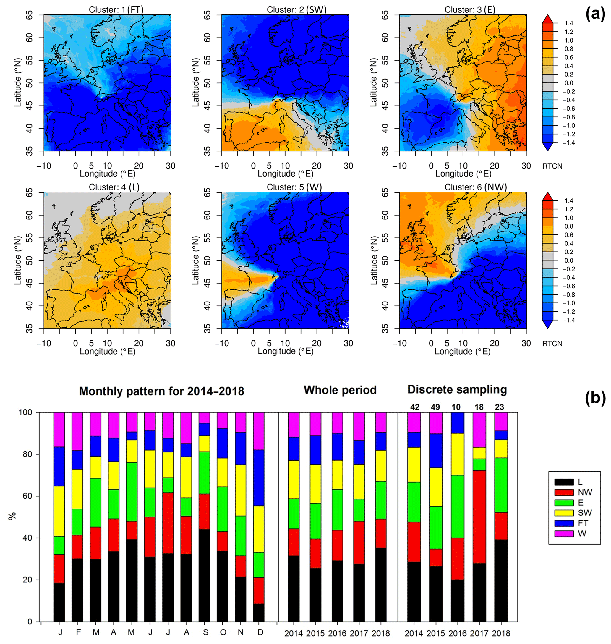
Figure 4(a) Clusters of air mass transport regimes for Jungfraujoch shown as normalized surface source sensitivities over our sampling period. Cluster abbreviations refer to Free Troposphere (FT), Southwest (SW), East (E), Local (L), West (W) and Northwest (NW). The normalization was done by calculating the difference between cluster-average source sensitivity and whole-period-average source sensitivities, divided by the period average. Orange colors indicate the main source regimes in each cluster, whereas blue colors indicate little to no influence on Jungfraujoch observations. The free tropospheric cluster showed lower than average surface sensitivity everywhere. (b) Cluster frequency of air mass transport regimes (%) shown as a monthly pattern (left) and interannual patterns for the whole periods (middle) and for the periods of discrete sampling (right). Numbers above the right figure indicate the total number of discrete samples per year.
3.4 Air mass origin and in situ measurements at Jungfraujoch
Back-trajectory simulations indicate six major transport clusters during 2014–2018, as shown in Fig. 4a. Four of these transport regimes (SW, E, L and NW) dominate, accounting for about 60 %–90 % coverage of the whole period. By contrast, the free troposphere cluster only represents 10 %–20 % of the data. Averaged monthly contributions of transport clusters are shown in Fig. 4b, with more pronounced impact by the L, E and NW regions in summer and stronger contribution by FT and SW in winter. The source patterns of the air masses at Jungfraujoch were generally consistent across the years in the present study. However, an apparent discrepancy was found for discrete sampling times in the last 2 years (e.g., particularly low contribution from SW), which is most likely due to the low and variable sampling frequency of the discrete sample collection (Fig. 4b).
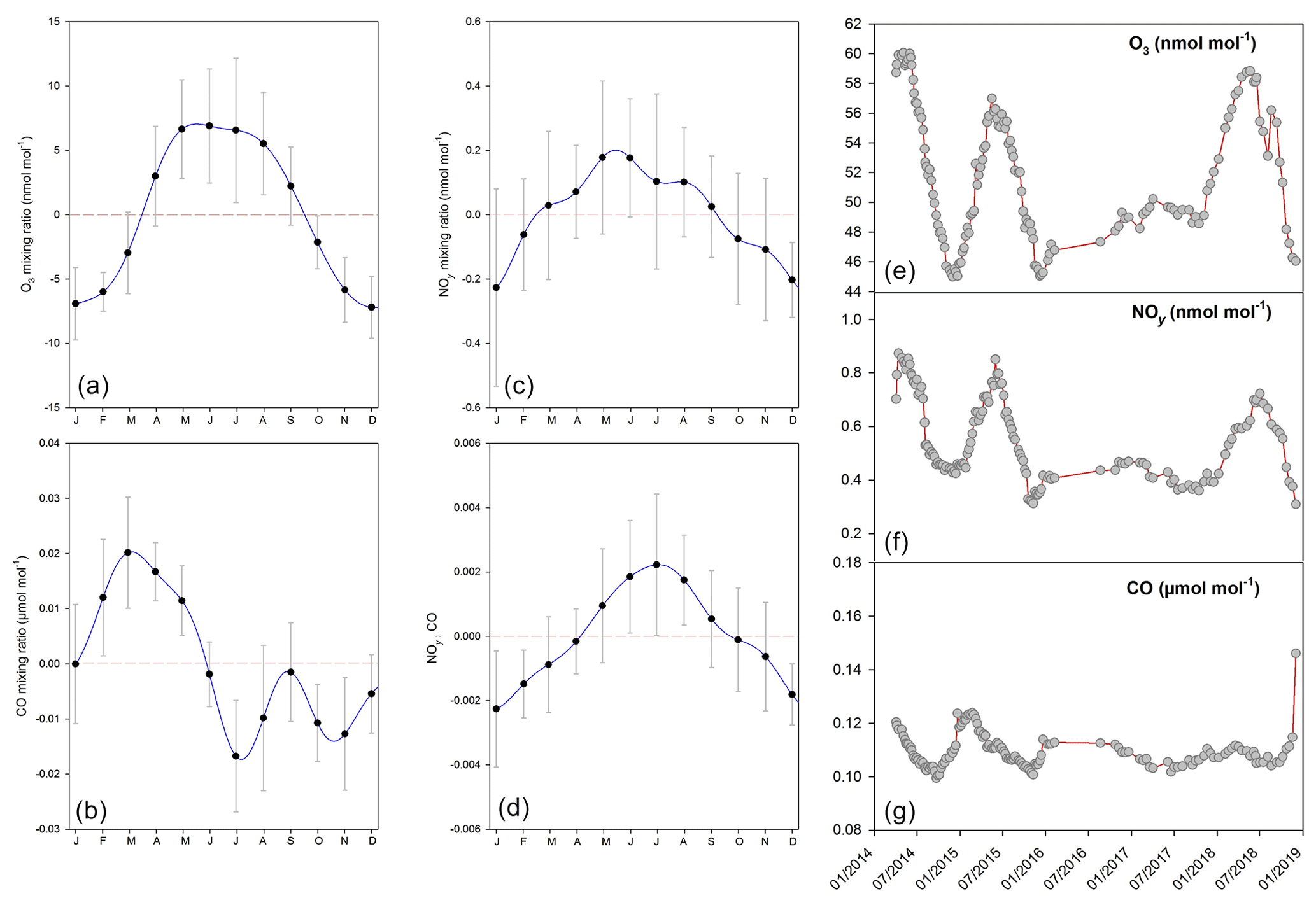
Figure 5(a–d) Seasonality of in situ measurements of O3, NOy and CO mixing ratios and NOy ∕ CO at Jungfraujoch; error bars represent the 1 standard deviation of monthly residuals from the NLS model simulation for time series. The 10 min data were used for seasonality analysis. (e–g) In situ measurements of O3, NOy and CO mixing ratios were averaged over the exact period of discrete sampling (∼40 min).
The detrended seasonal variability of in situ measurements indicates summer maxima for NOy mixing ratios as well as NOy-to-CO ratios at Jungfraujoch (Fig. 5). This likely indicates stronger exchange with the polluted planetary boundary layer in summer (Herrmann et al., 2015; Zellweger et al., 2003), which is consistent with the seasonal pattern of air mass footprint derived from back-trajectory simulations. The late spring-to-summer maxima for O3 mixing ratios may be attributed to air mixing with stratosphere and/or planetary boundary layer, similar to the findings from a previous study at Jungfraujoch (Tarasova et al., 2009). On the other hand, CO shows a maximum in early spring and decreases in summer when its atmospheric lifetime is shortest. Atmospheric O3, NOy and CO measurements during our discrete sampling periods also well represented seasonal variability shown for in situ measurements, except for 2016–2017 where there was a 5-month sampling gap (Fig. 5).
Comparisons of air mass footprints as well as O3, NOy and CO mixing ratios between in situ and discrete sampling indicate that the discrete sampling covers the main air source regions and variabilities in local pollution and free troposphere fairly well (Figs. 4 and 5). In the second phase (2016–2018), the less frequent sampling impedes evaluation of the seasonal and interannual variabilities.
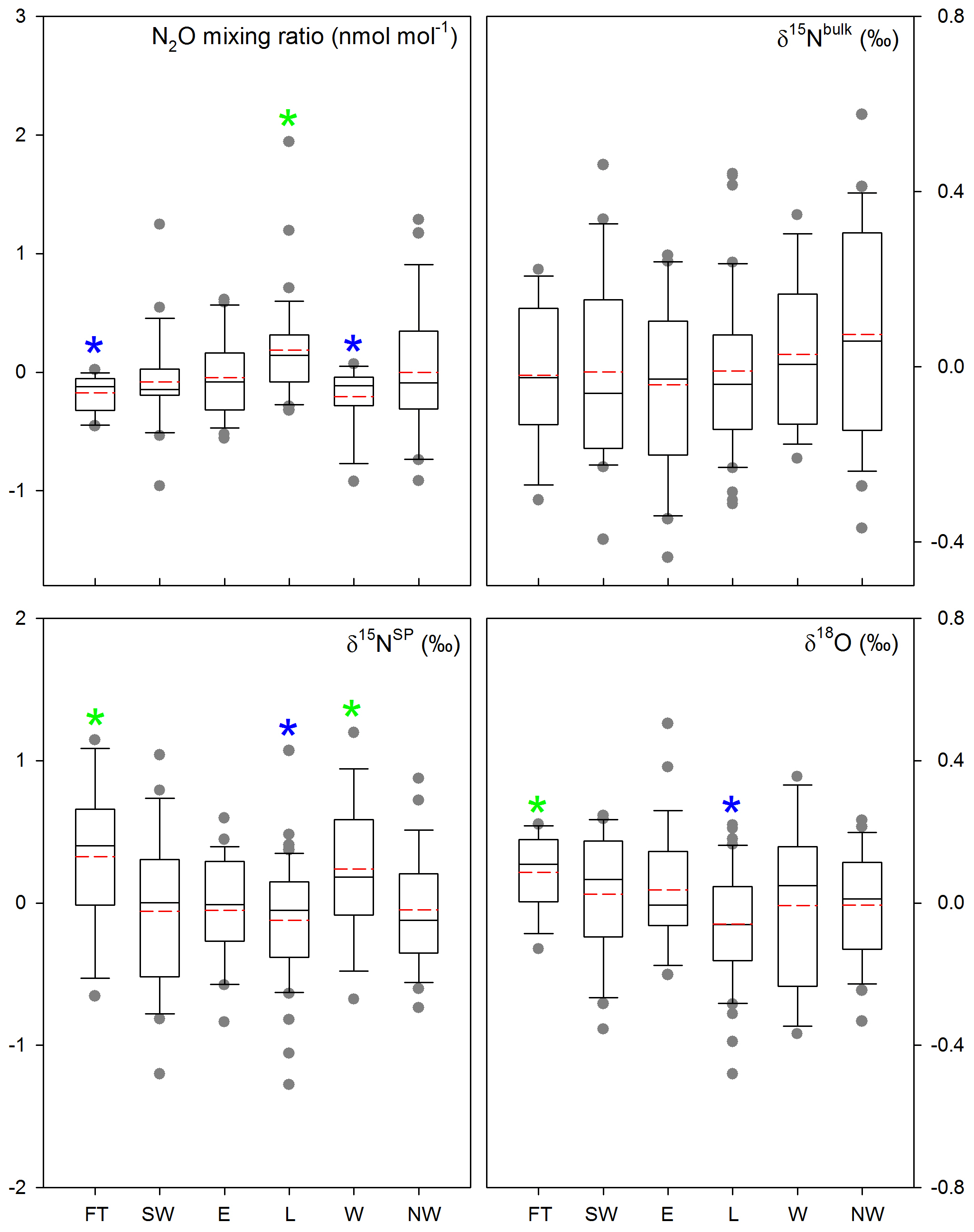
Figure 6Comparison of N2O mixing ratios and isotopic signatures (with linear trends removed) for the six air mass footprint clusters used in the present study. Green and blue stars indicate significantly larger and smaller values than the others, respectively; red dashed lines indicate mean levels; grey points indicate outliers.
3.5 Relationship between N2O isotopic signatures and air mass footprints
We categorized N2O mixing ratio and isotopic signature time series into subsets based on the six air mass transport clusters. One-way ANOVA among clusters indicates that N2O mixing ratios in air masses originating from cluster L were significantly higher and those from clusters FT and W were significantly lower than the others (Fig. 6). In accordance with the pattern found for mixing ratios, δ15NSP and δ18O were high for cluster FT, and low for cluster L. For δ15Nbulk, little difference between transport clusters was detected.
4.1 Quality assurance of isotopic measurements
This study reports the first results of background N2O isotopic measurements based on a laser spectroscopic technique. Benefiting from the preconcentration process, we achieved measurement repeatability for a target gas of 0.10 ‰–0.20 ‰ for δ15Nbulk and δ18O (Fig. S2), which is comparable to that of IRMS measurements of ambient atmosphere (Park et al., 2012; Prokopiou et al., 2017; Röckmann et al., 2003; Toyoda et al., 2013). The long-term robustness of our technique is adequate for disentangling both seasonal and interannual temporal variability as shown in Fig. 2. In particular, our repeatability of target measurements for δ15NSP (0.15 ‰–0.25 ‰) appears to be better than previous studies measuring background atmosphere or firn air (0.8 ‰, Park et al., 2012; 0.3 ‰, Prokopiou et al., 2017; 0.3 ‰, Toyoda et al., 2013).
4.2 Seasonal variabilities of atmospheric N2O isotopic composition
In situ measurements of N2O mixing ratios showed a clear early summer maximum and late summer minimum (Fig. 1). Such a seasonal pattern was previously found for a number of NOAA and AGAGE sites analyzing long-term N2O records in the NH (Jiang et al., 2007; Nevison et al., 2011). One explanation of the late-summer minimum is a strong influence of the STE process in this period, which transports N2O-depleted but isotopically enriched air downward from the stratosphere into the troposphere (Park et al., 2012; Snider et al., 2015b). During the late summer at Jungfraujoch, we find strong enrichment of 15N in atmospheric N2O according to the detrended seasonality for the whole dataset (Fig. 3). This is supported by a FLEXPART model simulation of the contribution of upper tropospheric air to Jungfraujoch station, showing highest contributions in August (Fig. S4; Stephan Henne, personal communication, 2019). At Hateruma Island, Japan, Toyoda et al. (2013) observed a seasonal pattern of atmospheric N2O mixing ratios, which is comparable with our study, but they found insignificant variations of isotopic composition. On the other hand, N2O seasonal variability could be influenced by oceanic emission sources (Jiang et al., 2007; Nevison et al., 2005), complicating the explanations for the observed temporal patterns. For example, in another study looking at archived air from Cape Grim, Australia, Park et al. (2012) detected an April–May minimum and a November–December maximum for N2O. This is expected for the SH, as STE is most prevalent in April (Nevison et al., 2011). They observed negative correlations of δ15Nbulk, δ15Nα and δ18O with N2O mixing ratios, appearing to support the idea that the STE process is responsible for seasonal variabilities in N2O mixing ratios and isotopic composition at Cape Grim. However, the seasonal cycle for δ15Nα was much larger than δ15Nbulk and δ18O, which could not be explained by STE alone. They suggested that the seasonal patterns of N2O isotopes at Cape Grim may be due to mixing between oceanic sources (high N2O with low 15N and 18O) and STE (low N2O with high 15N and 18O) (Nevison et al., 2011; Park et al., 2012). However, because we observed a concurrent minimum of δ15NSP and maximum of δ15Nbulk in July–August with low N2O at Jungfraujoch (Fig. 3), additional mechanisms must be considered here.
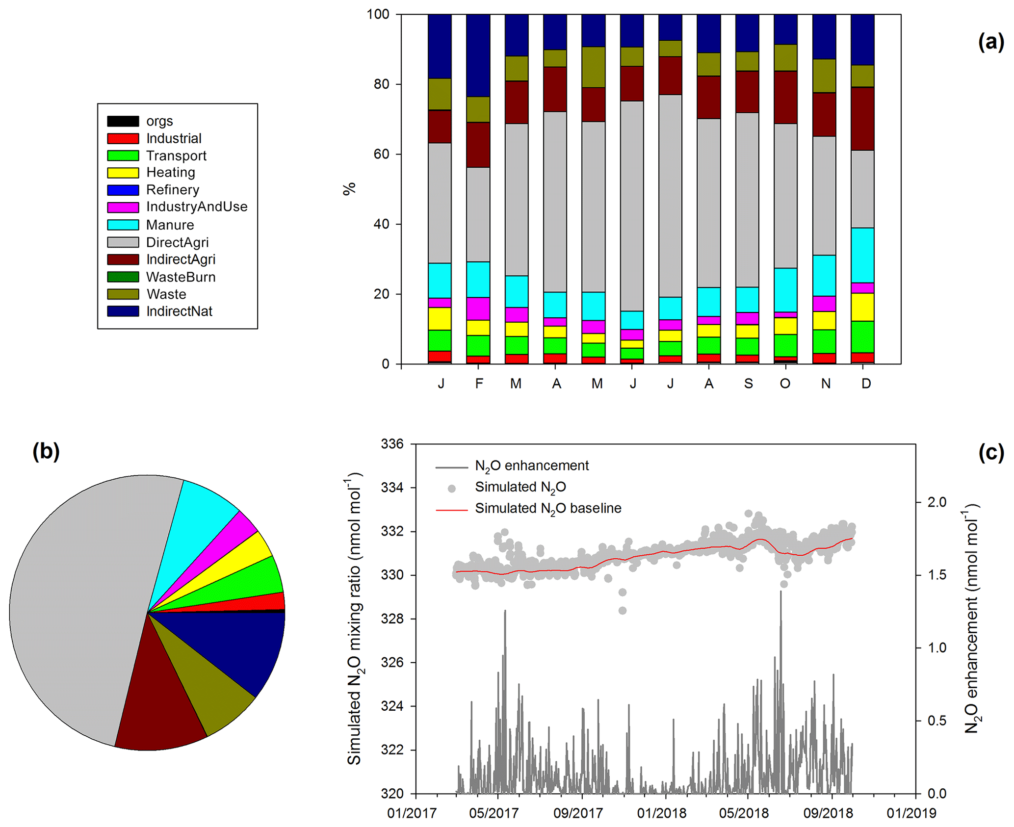
Figure 7(a) Mean monthly stacked-bar plots of source contributions (%) to atmospheric N2O at Jungfraujoch derived from inversion modeling. (b) Overall contributions of N2O sources responsible for emission to Jungfraujoch. (c) Simulated 3-hourly N2O mixing ratios, N2O mixing ratio baseline and N2O enhancements in units of nanomole per mole (nmol mol−1).
Regional model simulations based on Swiss N2O emissions derived from the inverse method were used to explore contributions from different sources to the variability in N2O enhancements at Jungfraujoch. As shown in Fig. 7a and b, soil emissions, including direct and indirect emissions from agricultural lands and emissions from (semi-)natural areas, account for more than 70 % of the total N2O enhancements, while manure and waste management contribute another 20 %. Total N2O enhancements appeared to be highest in May to July (Fig. 7c), in accordance with the highest contribution by soil emissions. The early-to-middle summer maximum in the simulated N2O enhancements is comparable with maximum of N2O mixing ratios in early summer as observed at Jungfraujoch (Fig. 1c). This underlines the importance of soil emission in accounting for atmospheric N2O variability (Saikawa et al., 2014). In late summer, the minimum of δ15NSP (Fig. 3) may be then attributed to the influence of soil emitted N2O, which has lower δ15NSP (7.2±3.8 ‰; Table 1) than the troposphere (Fig. 2). However, the STE process, which resulted in the minimum of N2O mixing ratio, likely contributes a positive isotope effect in the meantime (Kaiser et al., 2006). In order to evaluate the combined effect of STE and soil emission on δ15NSP in late summer, we applied a mixing calculation. Such an estimate was made based on the approximated N2O enhancement or depletion contributed by the two processes and the assumed isotope effects (see more details in the “Materials and methods” section). The mixing calculation indicated an overall isotope effect of about 0.01 ‰, which is extremely small and below our analytic precision. This practice suggests that it is still challenging to build a direct link between N2O sources and processes and the observed isotope signature in the background atmosphere. It is also noteworthy that the δ15NSP used in the calculation (7.2±3.8 ‰) may underestimate the isotope effects of soil emission, given that denitrification, as a major N2O process in soils, produces N2O with δ15NSP close to 0 ‰ (Sutka et al., 2006). Previous field studies have demonstrated that low-δ15NSP N2O emissions (∼0 ‰), i.e., following the denitrification pathway, predominates during summer periods at Swiss (Wolf et al., 2015) and German (Ibraim et al., 2019) grasslands. By contrast, the influence of biogeochemical processes (nitrification and denitrification) on δ15Nbulk is generally smaller than that on δ15NSP (Toyoda et al., 2011), and such an effect on δ15Nbulk are usually overwritten by the wide range of isotopic signatures in soil N substrates (Sutka et al., 2006). Hence, given the distinct δ15Nbulk maximum and N2O minimum in late summer during our observation (Figs. 1 and 3), we suggest that the STE process is mainly responsible for the seasonal variability in δ15Nbulk.
The footprint analyses based on air mass residence time revealed a seasonal pattern, with a higher contribution of background air from the FT and SW regions in winter and more pronounced contribution of local planetary boundary layer air from the L, E and NW regions in summer (Fig. 4b). The higher frequency of air mass footprints recently in contact with the surface in summer is consistent with inverse modeling results, indicating a larger contribution of soil N2O emissions in June–July (Fig. 7). For the air mass regime representing the free troposphere, N2O mixing ratios observed at Jungfraujoch were significantly below the average, while δ15NSP and δ18O were higher (Fig. 6). By contrast, the local cluster (L) representing a strong impact from the planetary boundary layer had higher N2O mixing ratios and lower isotopic signatures (except δ15Nbulk) than the other source regions. In addition, the ratio of NOy to CO, which is a more straightforward indicator of the free troposphere (Zellweger et al., 2003), shows significant negative correlations with δ15NSP and δ18O but not with δ15Nbulk (Fig. 8). This further suggests that the seasonal variability of δ15NSP and δ18O observed at Jungfraujoch is most likely influenced by ground-derived emissions, while fluctuations in N2O mixing ratios and δ15Nbulk are possibly driven by STE.
Considering the complexity in mechanisms responsible for N2O isotopic variations, we strongly recommend more field measurements of N2O isotopic signatures at higher frequency and at different background sites in order to cover spatial and temporal variability in N2O sources. For example, in the second phase, we only detected a significant seasonality of δ15NSP, with a minimum in July, which is 1 month earlier than the summer minimum found for the whole dataset (Fig. 3). This may be attributed to a difference in source regions, as Northwest regions appeared to be significantly more important during 2017 (second phase). However, due to low sampling frequency, it is challenging to overcome the large uncertainty in seasonality analysis for a 2-year period such as the second phase.
Based on our bottom-up approach, we simulated isotopic signatures for the overall N2O sources responsible for the N2O mixing ratio increase in the atmosphere (Fig. 9). However, the interpretation of simulated versus observed variability in N2O isotopic composition was difficult, except for the somewhat similar patterns in δ18O. Our results suggest a limitation in the current knowledge and literature values on isotopic signatures of most N2O sources. In addition, most N2O sources may not exhibit a well-defined isotopic signature but a range of values regulated under a number of processes and environmental factors. For example, isotopic signatures of soil-derived N2O are often determined by an interaction of several soil and climatic factors. It might be possible in the future to model these changes implementing isotopes in ecosystem models, as recently demonstrated by Denk et al. (2019).
4.3 Interannual trends of atmospheric N2O isotopic composition
Over a period of almost 5 years, our observations show an interannual increase in N2O mixing ratio and decrease in δ15Nbulk (Fig. 10). This is to be expected, assuming that the atmospheric N2O increase is primarily attributed to anthropogenic sources, which emit isotopically lighter N2O relative to the tropospheric background (Table 1) (Rahn and Wahlen, 2000). Compared to several studies on firn air (Ishijima et al., 2007; Röckmann et al., 2003) and surface air (Park et al., 2012; Röckmann and Levin, 2005; Toyoda et al., 2013), the rate of decrease for δ15Nbulk at Jungfraujoch is relatively high (−0.05 ‰ a−1 to −0.06 ‰ a−1, Table 3). Such a discrepancy in the δ15Nbulk trend could be due to a large contribution of terrestrial N2O emission from the European continent to Jungfraujoch (Figs. 6 and 7), as N2O originating from soil emissions is significantly more isotopically depleted than that of oceanic sources (Snider et al., 2015b). Nevertheless, our observation period is shorter than that of other studies, so the interannual trends determined here are more likely affected by year-to-year variability. Among all reported records, the decrease of δ15Nbulk observed at Hateruma Island was the most up-to-date and smallest (−0.020 ‰ a−1–0.026 ‰ a−1) (Toyoda et al., 2013). The authors argued that the smaller declining trend for δ15Nbulk may be explained by the recent increase in anthropogenic isotopic ratios particularly for agricultural N2O emissions; although, Ishijima et al. (2007) suggested a decline in both δ15Nbulk and δ18O in anthropogenic N2O from 1952–1970 to 1970–2001 based on inverse modeling.
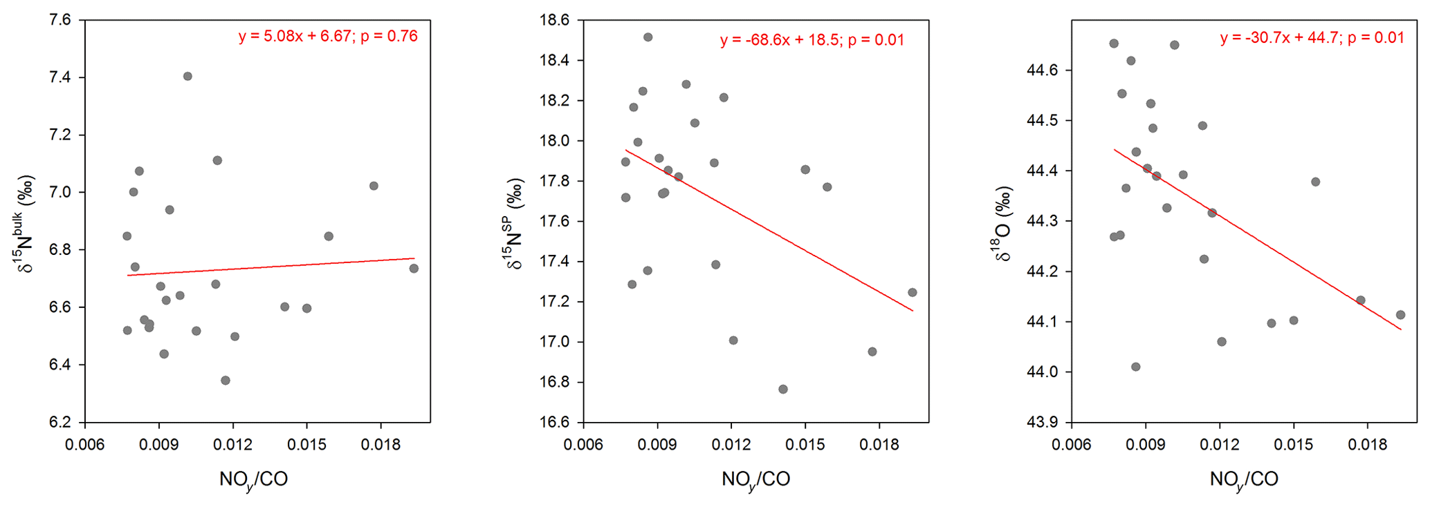
Figure 8Relationship between the NOy to CO ratios and isotopic signatures of N2O; only data points with NOy ∕ CO > 0.007 are presented here (which refer to scenarios with strong pollution from local air).
For the interannual trends observed at Jungfraujoch, it is noteworthy to point out that our observations covering a rather short period may lead to large uncertainties despite statistical significance. The discrepancy found in the trends between the first and second phases indicates that variability of N2O isotopic composition is likely to obscure interannual trends over shorter periods (Toyoda et al., 2013). Hence, extended time series of isotopic measurements are needed to reevaluate, for example, the observed tendency of increase in δ18O and δ15NSP at Jungfraujoch (Table 3; only significant during the first phase). For δ18O of atmospheric N2O, a generally declining trend smaller than that of δ15Nbulk has been indicated by a number of observations (Bernard et al., 2006; Ishijima et al., 2007; Park et al., 2012; Röckmann et al., 2003; Röckmann and Levin, 2005). This is expected as δ18O of anthropogenic N2O is not much different from that of the natural background, assuming that the oxygen atom in N2O is largely derived from soil water and ambient oxygen during production (Rahn and Wahlen, 2000).
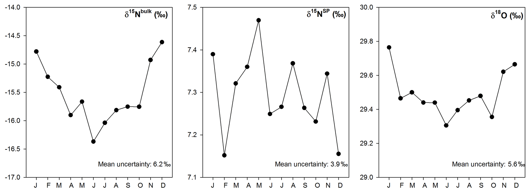
Figure 9Simulated seasonal variations of isotopic signatures for overall N2O sources based on the bottom-up approach; uncertainties shown in figures are comparable to the ranges of isotopic signatures for variable sources as found in literature.
It is still a challenging task to disentangle interannual trends of δ15NSP-N2O in the background atmosphere, due to limitations in analytical repeatability and precision (Harris et al., 2017; Mohn et al., 2014). Past results have reached inconsistent conclusions, showing positive (Bernard et al., 2006; Park et al., 2012; Prokopiou et al., 2017; Röckmann and Levin, 2005) or negative (Röckmann et al., 2003; Toyoda et al., 2013) trends of similar magnitude (Fig. 10). On the one hand, the negative trend in δ15NSP could be explained by the significantly lower δ15NSP from anthropogenic sources (e.g., agricultural sources; Table 1) than of the tropospheric background (near 18 ‰; Fig. 10). On the other hand, Park et al. (2012) suggested that the increase of δ15NSP in the atmospheric N2O may reflect a global increase in importance of the contribution by nitrification (high-δ15NSP process) to agricultural N2O emissions. This is based on the assumption that the growth of N2O emissions is largely due to enhanced fertilizer application, which promotes nitrification activity (Pérez et al., 2001; Tian et al., 2019). The observed mean increase rate of 0.02 ‰ a−1 for δ15NSP by Park et al. (2012) could then be translated into an increase of 13 %–23 % for the relative amount of nitrification-derived N2O between 1750 and 2005. However, this should be further evaluated with more frequent sampling (Park et al. (2012) only sampled 1–6 times per year) and tested with isotopic measurements across the NH, where agricultural N2O emissions are more dominant than in the SH. In addition, the strong seasonal pattern of δ15NSP at Jungfraujoch suggests that seasonal variations of δ15NSP in response to climatic or source factors are crucial and must be taken into consideration for evaluating interannual δ15NSP trends.
4.4 Simulated anthropogenic N2O sources with the two-box model and comparison with other studies
To further evaluate anthropogenic source signatures of N2O isotopic composition, we applied a two-box model representing a well-mixed troposphere and stratosphere (Röckmann et al., 2003; Schilt et al., 2014; Sowers et al., 2002). The model runs with the whole dataset and the dataset filtered for free troposphere only (Table 4) exhibit statistically identical results, supporting that our model estimates, with observations at Jungfraujoch, are representative of the background atmosphere. The simulated trends of the N2O mixing ratios and isotopic composition show a gradual increase in N2O and decrease in the isotopic signatures (see Fig. 10), which agree with existing observations within the model uncertainty. However, this does not hold for individual studies considered separately. For example, the N2O mixing ratios observed by Röckmann et al. (2003) and Prokopiou et al. (2017) would lead to a higher preindustrial N2O compared to our model simulation, which is likely due to the uncertainty in the firn air records (Prokopiou et al., 2017).
Table 5Isotopic signatures for the overall, anthropogenic and major N2O sources contributing to N2O variations at Jungfraujoch. Source signatures were estimated based on a bottom-up approach, with literature-derived isotopic signatures and fluxes for variable sources under the Swiss Meteotest emission inventory.
∗ “Waste” sources consist of both wastewater treatment and agricultural waste burning (biomass burning).
We compared the anthropogenic isotopic signatures determined by our two-box model with other similar studies in Table 4. Our estimates generally lie within the ranges given in the earlier studies (Ishijima et al., 2007; Park et al., 2012; Prokopiou et al., 2017; Röckmann et al., 2003; Sowers et al., 2002; Toyoda et al., 2013). However, isotopic signatures of N2O sources estimated for 2018 in this study are higher in δ15Nbulk and δ18O (by 4 ‰–8 ‰), and lower in δ15NSP (by 2 ‰–7 ‰), than model estimates for the early 2000s from two other studies from the SH (Park et al., 2012; Prokopiou et al., 2017). Such differences in δ15Nbulk and δ18O could be related to interhemispheric differences, as the relative contributions of N2O sources vary between the two hemispheres (Toyoda et al., 2013). Also, more interestingly, this could suggest a shift in the N2O source isotopic signatures over the last few decades. For example, an increase of δ15Nbulk in anthropogenic N2O sources over time may be attributed to growing contributions of other industrial or waste sources with high δ15Nbulk (Prokopiou et al., 2017). In addition, if the assumption of increasing δ15Nbulk and decreasing δ15NSP in anthropogenic N2O sources over time holds, it points to a recently growing contribution of denitrification relative to nitrification to the global atmospheric N2O increase (Sutka et al., 2006; Toyoda et al., 2013). By contrast, Park et al. (2012) and Prokopiou et al. (2017) proposed an increasing importance of nitrification for anthropogenic N2O emissions based on the increasing δ15NSP trend since 1940. This may suggest that a strong climate change feedback has recently resulted in significant shifts in N2O source process, hence twisting the isotopic signatures of anthropogenic sources (Griffis et al., 2017; Xu-Ri et al., 2012). Alternatively, the uncertainty in determining N2O isotopic signatures in the background atmosphere and interlaboratory comparability may play a role in the observed discrepancy.
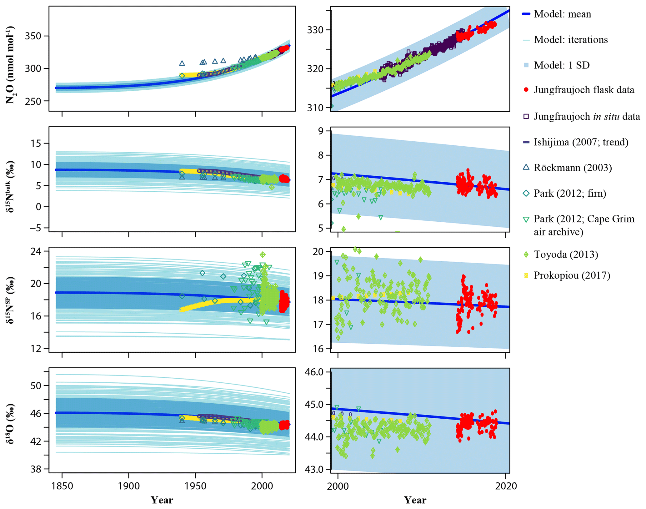
Figure 10Two-box model results showing the influence of anthropogenic emissions on N2O mixing ratio and isotopic composition in the troposphere. Left: full time range from the start of the anthropogenic period (1845) to present day; Right: zoom to the last 2 decades. Isotopic measurements at Jungfraujoch were used as the only constraint of current tropospheric N2O isotopic composition for the model. See the Materials and methods section as well as the Supplement for more details and other input parameters. Atmospheric as well as firn air measurements of δ15Nbulk, δ15NSP and δ18O from the literature are presented for comparison. Shaded blue areas indicate 1 standard deviation of the model iterations.
Given the strong heterogeneity in source contributions to N2O emissions around the globe (Saikawa et al., 2014), current two- and four-box model estimates based on observations at individual sites or regions are likely to reflect latitudinal or even interhemispheric differences in anthropogenic isotopic signatures. On the other hand, previous discussions of the model sensitivities by Röckmann et al. (2003) and Toyoda et al. (2013) have suggested that anthropogenic isotopic values are most sensitive to the trends in tropospheric isotopic values and the relative difference in tropospheric isotopic values between present and preindustrial times. For example, given the similar parameters used for preindustrial times as our study, Park et al. (2012) observed much lower δ15Nbulk in the recent troposphere than in our case, and hence resulting in significantly lower δ15Nbulk for the anthropogenic source. Furthermore, Park et al. (2012) and Prokopiou et al. (2017) simulated a positive trend in δ15NSP relative to preindustrial times, which in return resulted in a much higher δ15NSP for the anthropogenic sources.
Using an alternative bottom-up approach, we estimated the anthropogenic source isotopic signatures based on the N2O emission inventory simulated for Jungfraujoch and published source isotopic signatures as summarized by Harris et al. (2017) (Table 1). The retrieved anthropogenic isotopic signatures (Table 5) were largely in agreement with the isotopic signature of agricultural soil emissions (Snider et al., 2015b; Wolf et al., 2015), indicating that this source could explain more than 60 % of the total N2O emissions. However, the anthropogenic isotopic signatures estimated by this approach were lower than the results from our two-box model (Table 4). In contrast, another similar bottom-up estimate based on the global N2O emission inventory (Toyoda et al., 2013) reported anthropogenic isotopic values that agree well with our box-model results. This may be explained by the different isotopic signatures used to describe agricultural N2O emissions, as those values used for the bottom-up estimates by Toyoda et al. (2013) were significantly lower (Toyoda et al., 2011) than those used in this study (Snider et al., 2015b; Wolf et al., 2015). Such bottom-up estimation suggests that more isotopic measurements of the background atmosphere from different regions, and better constraints on individual anthropogenic (especially agricultural) N2O isotopic signatures, are necessary for a better representation of N2O isotopic composition in atmospheric modeling studies.
With the recently developed laser spectroscopic technique coupled with a preconcentration device, we achieved good repeatability in measurements of N2O isotopic composition from the background atmosphere at Jungfraujoch, Switzerland. This time series covered a period of 5 years and showed a distinct seasonality, with δ15Nbulk maxima and δ15NSP minima in late summer, associated with the lowest N2O mixing ratios over the year. The seasonal fluctuation of δ15Nbulk was associated with the stratosphere–troposphere exchange process, in agreement with other monitoring networks (Nevison et al., 2011), while the contrasting depletion of δ15NSP in later summer is possibly a combined result of STE and agricultural emissions, with the latter being more important. The analyses of air mass transport regimes together with the simulation of N2O enhancements for Jungfraujoch supported our explanations and highlighted that the fluctuation between the free troposphere and local contributions dominated by soil emission drives the seasonality of δ15NSP and δ18O as observed at Jungfraujoch.
We found statistically significant interannual trends for δ15Nbulk, which is expected as anthropogenic N2O sources are characterized by low 15N abundance. For δ15NSP and δ18O, interannual trends were highly uncertain and possibly masked by their large temporal variabilities. Using a two-box model approach, we simulated the evolution of N2O isotopic composition from preindustrial times to the present. This model suggests an overall decreasing trend for all isotopic deltas in conjunction with the atmospheric N2O increase. The anthropogenic source signatures given by the model generally agreed with previous studies. However, these model results are still sensitive to the ranges and trends of the observed N2O isotopic signatures in the present troposphere. In the future, more extended records of high-precision N2O isotopic measurements and application of multiple-box modeling approaches (Rigby et al., 2013) are necessary to account for the global N2O budget and evolution of anthropogenic sources.
Data for this study have been deposited in a general data repository (https://doi.org/10.6084/m9.figshare.12032760.v1, Yu et al., 2020).
The supplement related to this article is available online at: https://doi.org/10.5194/acp-20-6495-2020-supplement.
LY, EH and JM led and designed this study. LY, EH, SE conducted sample collection at Jungfraujoch; LY and EH analyzed discrete samples at Empa; MS and CZ contributed in situ measurements of N2O, NOy, CO and O3 at Jungfraujoch; LY, EH and SH performed data analyses for the time series and conducted model simulations. LY wrote the main part of the article; EH, SH and JM were involved in the revisions of the article and commenting. SE, MS, LE and CZ were also involved in scientific discussion and commenting on the article.
The authors declare that they have no conflict of interest.
We are thankful to the research infrastructure provided by the high-altitude research stations Jungfraujoch and Gornergrat. We are grateful to the help from the custodians (Martin and Joan Fischer and Ruedi and Christine Käser) at the research station of Jungfraujoch. We would like to thank Simon Wyss, Kerstin Zeyer, Patrik Zanchetta and Flurin Dietz for their support with the sample collection as well as laboratory assistance. NABEL is operated by Empa in collaboration with the Swiss Federal Office for the Environment. Sakae Toyoda and Naohiro Yoshida from Tokyo Institute of Technology are acknowledged for their analyses of the applied reference standards. This study was financially supported by the Swiss National Science Foundation (grant number 200021_163075) and the Swiss contribution to the Integrated Carbon Observation System (ICOS) Research Infrastructure (ICOS-CH). ICOS-CH is funded by the Swiss National Science Foundation and in-house contributions. Longfei Yu was additionally supported by the EMPAPOSTDOCS-II program, which receives funding from the European Union's Horizon 2020 research and innovation program under the Marie Skłodowska-Curie grant agreement number 754364.
This research has been supported by the Swiss National Science Foundation (grant no. 200021_163075) and the European Union's Horizon 2020 research and innovation program (Marie Skłodowska-Curie grant agreement number 754364).
This paper was edited by Jan Kaiser and reviewed by two anonymous referees.
Appenzeller, C., Begert, M., Zenklusen, E., and Scherrer, S. C.: Monitoring climate at Jungfraujoch in the high Swiss Alpine region, Sci. Total Environ., 391, 262–268, https://doi.org/10.1016/j.scitotenv.2007.10.005, 2008.
Bernard, S., Röckmann, T., Kaiser, J., Barnola, J.-M., Fischer, H., Blunier, T., and Chappellaz, J.: Constraints on N2O budget changes since pre-industrial time from new firn air and ice core isotope measurements, Atmos. Chem. Phys., 6, 493–503, https://doi.org/10.5194/acp-6-493-2006, 2006.
Bourbonnais, A., Letscher, R. T., Bange, H. W., Échevin, V., Larkum, J., Mohn, J., Yoshida, N., and Altabet, M. A.: N2O production and consumption from stable isotopic and concentration data in the Peruvian coastal upwelling system, Global Biogeochem. Cy., 31, 678–698, https://doi.org/10.1002/2016GB005567, 2017.
Buchmann, B., Hueglin, C., Reimann, S., Vollmer, M. K., Steinbacher, M., and Emmenegger, L.: Reactive gases, ozone depleting substances and greenhouse gases, in: From weather observations to atmospheric and climate sciences in Switzerland, edited by: Willemse, S. and Furger, M., vdf Hochschulverlag AG, Dübendorf, Switzerland, 2016.
Bukowiecki, N., Weingartner, E., Gysel, M., Coen, M. C., Zieger, P., Herrmann, E., Steinbacher, M., Gäggeler, H. W., and Baltensperger, U.: A review of more than 20 years of aerosol observation at the high altitude research station Jungfraujoch, Switzerland (3580 m a.s.l.), Aerosol Air Qual. Res., 16, 764–788, https://doi.org/10.4209/aaqr.2015.05.0305, 2016.
Butterbach-Bahl, K., Baggs, E. M., Dannenmann, M., Kiese, R., and Zechmeister-Boltenstern, S.: Nitrous oxide emissions from soils: how well do we understand the processes and their controls?, Philos. T. Roy. Soc. B, 368, 20130122, https://doi.org/10.1098/rstb.2013.0122, 2013.
Decock, C. and Six, J.: How reliable is the intramolecular distribution of 15N in N2O to source partition N2O emitted from soil?, Soil Biol. Biochem., 65, 114–127, https://doi.org/10.1016/j.soilbio.2013.05.012, 2013.
Denk, T. R. A., Mohn, J., Decock, C., Lewicka-Szczebak, D., Harris, E., Butterbach-Bahl, K., Kiese, R., and Wolf, B.: The nitrogen cycle: A review of isotope effects and isotope modeling approaches, Soil Biol. Biochem., 105, 121–137, https://doi.org/10.1016/j.soilbio.2016.11.015, 2017.
Denk, T. R. A., Kraus, D., Kiese, R., Butterbach-Bahl, K., and Wolf, B.: Constraining N cycling in the ecosystem model LandscapeDNDC with the stable isotope model SIMONE, Ecology, 100, c02675, https://doi.org/10.1002/ecy.2675, 2019.
Fowler, D., Steadman, C. E., Stevenson, D., Coyle, M., Rees, R. M., Skiba, U. M., Sutton, M. A., Cape, J. N., Dore, A. J., Vieno, M., Simpson, D., Zaehle, S., Stocker, B. D., Rinaldi, M., Facchini, M. C., Flechard, C. R., Nemitz, E., Twigg, M., Erisman, J. W., Butterbach-Bahl, K., and Galloway, J. N.: Effects of global change during the 21st century on the nitrogen cycle, Atmos. Chem. Phys., 15, 13849–13893, https://doi.org/10.5194/acp-15-13849-2015, 2015.
Fujii, A., Toyoda, S., Yoshida, O., Watanabe, S., Sasaki, K., and Yoshida, N.: Distribution of nitrous oxide dissolved in water masses in the eastern subtropical North Pacific and its origin inferred from isotopomer analysis, J. Oceanogr., 69, 147–157, https://doi.org/10.1007/s10872-012-0162-4, 2013.
Griffis, T. J., Chen, Z., Baker, J. M., Wood, J. D., Millet, D. B., Lee, X., Venterea, R. T., and Turner, P. A.: Nitrous oxide emissions are enhanced in a warmer and wetter world, P. Natl. Acad. Sci. USA, 114, 12081–12085, https://doi.org/10.1073/pnas.1704552114, 2017.
Hall, B. D., Dutton, G. S., and Elkins, J. W.: The NOAA nitrous oxide standard scale for atmospheric observations, J. Geophys. Res.-Atmos., 112, 1–9, https://doi.org/10.1029/2006JD007954, 2007.
Harris, E. J., Nelson, D. D., Olsewski, W., Zahniser, M., Potter, E., Mcmanus, B. J., Whitehill, A., Prinn, R. G., Ono, S., and Harris, E.: Development of a spectroscopic technique for continuous online monitoring of oxygen and site-specific nitrogen isotopic com, Anal. Chem., 86, 1726–1734, 2014.
Harris, E., Zeyer, K., Kegel, R., Müller, B., Emmenegger, L., and Mohn, J.: Nitrous oxide and methane emissions and nitrous oxide isotopic composition from waste incineration in Switzerland, J. Waste Manag., 35, 135–140, https://doi.org/10.1016/j.wasman.2014.10.016, 2015.
Harris, E., Ibraim, E., Henne, S., Hüglin, C., Zellweger, C., Tuzson, B., Emmenegger, L., and Mohn, J.: Tracking nitrous oxide emission processes at a suburban site with semicontinuous, in situ measurements of isotopic composition, J. Geophys. Res.-Atmos., 122, 1850–1870, https://doi.org/10.1002/2016JD025906, 2017.
Heil, J., Wolf, B., Brüggemann, N., Emmenegger, L., Tuzson, B., Vereecken, H., and Mohn, J.: Site-specific 15N isotopic signatures of abiotically produced N2O, Geochim. Cosmochim. Ac., 139, 72–82, https://doi.org/10.1016/j.gca.2014.04.037, 2014.
Henne, S., Brunner, D., Folini, D., Solberg, S., Klausen, J., and Buchmann, B.: Assessment of parameters describing representativeness of air quality in-situ measurement sites, Atmos. Chem. Phys., 10, 3561–3581, https://doi.org/10.5194/acp-10-3561-2010, 2010.
Henne, S., Brunner, D., Oney, B., Leuenberger, M., Eugster, W., Bamberger, I., Meinhardt, F., Steinbacher, M., and Emmenegger, L.: Validation of the Swiss methane emission inventory by atmospheric observations and inverse modelling, Atmos. Chem. Phys., 16, 3683–3710, https://doi.org/10.5194/acp-16-3683-2016, 2016.
Henne, S., Mohn, J., and Brunner, D.: Quantification of Swiss nitrous oxide emissions through atmospheric observations and inverse modelling, Final Report, Project of FOEN, Swiss Federal Office for the Environment, Dübendorf, Switzerland, 2019.
Herrmann, E., Weingartner, E., Henne, S., Vuilleumier, L., Bukowiecki, N., Steinbacher, M., Conen, F., Coen, M. C., Hammer, E., Juranyi, Z., Baltensperger, U., and Gysel, M.: Analysis of long-term aerosol size distribution data from Jungfraujoch with emphasis on free tropospheric conditions, cloud influence, and air mass transport, J. Geophys. Res.-Atmos., 120, 1751–1762, https://doi.org/10.1002/2015JD023660, 2015.
Ibraim, E., Wolf, B., Harris, E., Gasche, R., Wei, J., Yu, L., Kiese, R., Eggleston, S., Butterbach-Bahl, K., Zeeman, M., Tuzson, B., Emmenegger, L., Six, J., Henne, S., and Mohn, J.: Attribution of N2O sources in a grassland soil with laser spectroscopy based isotopocule analysis, Biogeosciences, 16, 3247–3266, https://doi.org/10.5194/bg-16-3247-2019, 2019.
Ishijima, K., Sugawara, S., Kawamura, K., Hashida, G., Morimoto, S., Murayama, S., Aoki, S., and Nakazawa, T.: Temporal variations of the atmospheric nitrous oxide concentration and its δ15N and δ18O for the latter half of the 20th century reconstructed from firn air analyses, J. Geophys. Res.-Atmos., 112, D03305, https://doi.org/10.1029/2006JD007208, 2007.
Janssens-Maenhout, G., Crippa, M., Guizzardi, D., Muntean, M., Schaaf, E., Dentener, F., Bergamaschi, P., Pagliari, V., Olivier, J. G. J., Peters, J. A. H. W., van Aardenne, J. A., Monni, S., Doering, U., Petrescu, A. M. R., Solazzo, E., and Oreggioni, G. D.: EDGAR v4.3.2 Global Atlas of the three major greenhouse gas emissions for the period 1970–2012, Earth Syst. Sci. Data, 11, 959–1002, https://doi.org/10.5194/essd-11-959-2019, 2019.
Jiang, X., Ku, W. L., Shia, R. L., Li, Q., Elkins, J. W., Prinn, R. G., and Yung, Y. L.: Seasonal cycle of N2O: Analysis of data, Global Biogeochem. Cy., 21, GB1006, https://doi.org/10.1029/2006GB002691, 2007.
JMA and WMO: World Meteorological Organization – Global Atmosphere Watch – World Data Centre for Greenhouse Gases, Data Summary, No. 42, 101 p., available at: https://gaw.kishou.go.jp/static/publications/summary/sum42/sum42.pdf, last access: October 2018.
Kaiser, J., Röckmann, T., and Brenninkmeijer, C. A. M.: Complete and accurate mass spectrometric isotope analysis of tropospheric nitrous oxide, J. Geophys. Res.-Atmos., 108, 4476, https://doi.org/10.1029/2003JD003613, 2003.
Kaiser, J., Engel, A., Borchers, R., and Röckmann, T.: Probing stratospheric transport and chemistry with new balloon and aircraft observations of the meridional and vertical N2O isotope distribution, Atmos. Chem. Phys., 6, 3535–3556, https://doi.org/10.5194/acp-6-3535-2006, 2006.
Keller, C. A., Hill, M., Vollmer, M. K., Henne, S., Brunner, D., Reimann, S., O'Doherty, S., Arduini, J., Maione, M., Ferenczi, Z., Haszpra, L., Manning, A. J., and Peter, T.: European emissions of halogenated greenhouse gases inferred from atmospheric measurements, Environ. Sci. Technol., 46, 217–225, https://doi.org/10.1021/es202453j, 2012.
Kim, K.-R. and Craig, H.: Nitrogen-15 and Oxygen-18 Characacteristics of Nitrous Oxide: A Global Perspective, Science, 262, 1855–1857, 1993.
Lebegue, B., Schmidt, M., Ramonet, M., Wastine, B., Yver Kwok, C., Laurent, O., Belviso, S., Guemri, A., Philippon, C., Smith, J., and Conil, S.: Comparison of nitrous oxide (N2O) analyzers for high-precision measurements of atmospheric mole fractions, Atmos. Meas. Tech., 9, 1221–1238, https://doi.org/10.5194/amt-9-1221-2016, 2016.
Logan, J. A., Staehelin, J., Megretskaia, I. A., Cammas, J. P., Thouret, V., Claude, H., De Backer, H., Steinbacher, M., Scheel, H. E., Stbi, R., Frhlich, M., and Derwent, R.: Changes in ozone over Europe: Analysis of ozone measurements from sondes, regular aircraft (MOZAIC) and alpine surface sites, J. Geophys. Res.-Atmos., 117, 1–23, https://doi.org/10.1029/2011JD016952, 2012.
Maeda, K., Toyoda, S., Shimojima, R., Osada, T., Hanajima, D., Morioka, R., and Yoshida, N.: Source of nitrous oxide emissions during the cow manure composting process as revealed by isotopomer analysis of and amoa abundance in betaproteobacterial ammonia-oxidizing bacteria, Appl. Environ. Microb., 76, 1555–1562, https://doi.org/10.1128/AEM.01394-09, 2010.
Mohn, J., Guggenheim, C., Tuzson, B., Vollmer, M. K., Toyoda, S., Yoshida, N., and Emmenegger, L.: A liquid nitrogen-free preconcentration unit for measurements of ambient N2O isotopomers by QCLAS, Atmos. Meas. Tech., 3, 609–618, https://doi.org/10.5194/amt-3-609-2010, 2010.
Mohn, J., Tuzson, B., Manninen, A., Yoshida, N., Toyoda, S., Brand, W. A., and Emmenegger, L.: Site selective real-time measurements of atmospheric N2O isotopomers by laser spectroscopy, Atmos. Meas. Tech., 5, 1601–1609, https://doi.org/10.5194/amt-5-1601-2012, 2012.
Mohn, J., Wolf, B., Toyoda, S., Lin, C. T., Liang, M. C., Brüggemann, N., Wissel, H., Steiker, A. E., Dyckmans, J., Szwec, L., Ostrom, N. E., Casciotti, K. L., Forbes, M., Giesemann, A., Well, R., Doucett, R. R., Yarnes, C. T., Ridley, A. R., Kaiser, J., and Yoshida, N.: Interlaboratory assessment of nitrous oxide isotopomer analysis by isotope ratio mass spectrometry and laser spectroscopy: Current status and perspectives, Rapid Commun. Mass Spec., 28, 1995–2007, https://doi.org/10.1002/rcm.6982, 2014.
Nevison, C. D., Keeling, R. F., Weiss, R. F., Popp, B. N., Jin, X., Fraser, P. J., Porter, L. W., and Hess, P. G.: Southern Ocean ventilation inferred from seasonal cycles of atmospehric N2O and O2∕N2 at Cape Grim, Tasmania, Tellus B, 57, 218–229, https://doi.org/10.1111/j.1600-0889.2005.00143.x, 2005.
Nevison, C. D., Dlugokencky, E., Dutton, G., Elkins, J. W., Fraser, P., Hall, B., Krummel, P. B., Langenfelds, R. L., O'Doherty, S., Prinn, R. G., Steele, L. P., and Weiss, R. F.: Exploring causes of interannual variability in the seasonal cycles of tropospheric nitrous oxide, Atmos. Chem. Phys., 11, 3713–3730, https://doi.org/10.5194/acp-11-3713-2011, 2011.
Ogawa, M. and Yoshida, N.: Intramolecular distribution of stable nitrogen and oxygen isotopes of nitrous oxide emitted during coal combustion, Chemosphere, 61, 877–887, https://doi.org/10.1016/j.chemosphere.2005.04.096, 2005a.
Ogawa, M. and Yoshida, N.: Nitrous oxide emission from the burning of agricultural residue, Atmos. Environ., 39, 3421–3429, https://doi.org/10.1016/j.atmosenv.2005.01.059, 2005b.
Ostrom, N. E., Gandhi, H., Coplen, T. B., Toyoda, S., Böhlke, J. K., Brand, W. A., Casciotti, K. L., Dyckmans, J., Giesemann, A., Mohn, J., Well, R., Yu, L., and Yoshida, N.: Preliminary assessment of stable nitrogen and oxygen isotopic composition of USGS51 and USGS52 nitrous oxide reference gases and perspectives on calibration needs, Rapid Commun. Mass Spec., 32, 1207–1214, https://doi.org/10.1002/rcm.8157, 2018.
Pandey Deolal, S., Brunner, D., Steinbacher, M., Weers, U., and Staehelin, J.: Long-term in situ measurements of NOx and NOy at Jungfraujoch 1998–2009: Time series analysis and evaluation, Atmos. Chem. Phys., 12, 2551–2566, https://doi.org/10.5194/acp-12-2551-2012, 2012.
Park, S., Croteau, P., Boering, K. A., Etheridge, D. M., Ferretti, D., Fraser, P. J., Kim, K.-R., Krummel, P. B., Langenfelds, R. L., van Ommen, T. D., Steele, L. P., and Trudinger, C. M.: Trends and seasonal cycles in the isotopic composition of nitrous oxide since 1940, Nat. Geosci., 5, 261–265, https://doi.org/10.1038/ngeo1421, 2012.
Pérez, T., Trumbore, S. E., Tyler, S. C., Matson, P. A., Ortiz-Monasterio, I., Rahn, T., and Griffiths, D. W. T.: Identifying the agricultural imprint on the global N2O budget using stable isotopes, J. Geophys. Res., 106, 9869–9878, https://doi.org/10.1179/1607845413y.0000000087, 2001.
Prather, M. J., Hsu, J., Deluca, N. M., Jackman, C. H., Oman, L. D., Douglass, A. R., Fleming, E. L., Strahan, S. E., Steenrod, S. D., Søvde, O. A., Isaksen, I. S. A., Froidevaux, L., and Funke, B.: Measuring and modeling the lifetime of nitrous oxide including its variability Michael, J. Geophys. Res.-Atmos., 120, 5693–5705, https://doi.org/10.1002/2015JD023267, 2015.
Prinn, R. G., Weiss, R. F., Arduini, J., Arnold, T., DeWitt, H. L., Fraser, P. J., Ganesan, A. L., Gasore, J., Harth, C. M., Hermansen, O., Kim, J., Krummel, P. B., Li, S., Loh, Z. M., Lunder, C. R., Maione, M., Manning, A. J., Miller, B. R., Mitrevski, B., Mühle, J., O'Doherty, S., Park, S., Reimann, S., Rigby, M., Saito, T., Salameh, P. K., Schmidt, R., Simmonds, P. G., Steele, L. P., Vollmer, M. K., Wang, R. H., Yao, B., Yokouchi, Y., Young, D., and Zhou, L.: History of chemically and radiatively important atmospheric gases from the Advanced Global Atmospheric Gases Experiment (AGAGE), Earth Syst. Sci. Data, 10, 985–1018, https://doi.org/10.5194/essd-10-985-2018, 2018.
Prokopiou, M., Martinerie, P., Sapart, C. J., Witrant, E., Monteil, G., Ishijima, K., Bernard, S., Kaiser, J., Levin, I., Blunier, T., Etheridge, D., Dlugokencky, E., van de Wal, R. S. W., and Röckmann, T.: Constraining N2 emissions since 1940 using firn air isotope measurements in both hemispheres, Atmos. Chem. Phys., 17, 4539–4564, https://doi.org/10.5194/acp-17-4539-2017, 2017.
Prokopiou, M., Sapart, C. J., Rosen, J., Sperlich, P., Blunier, T., Brook, E., van de Wal, R. S. W. and Röckmann, T.: Changes in the Isotopic Signature of Atmospheric Nitrous Oxide and Its Global Average Source During the Last Three Millennia, J. Geophys. Res.-Atmos., 123, 1–17, https://doi.org/10.1029/2018JD029008, 2018.
Rahn, T. and Wahlen, M.: A reassessment of the global isotopic budget of atmospheric nitrous oxide, Global Biogeochem. Cy., 14, 537–543, https://doi.org/10.1029/1999GB900070, 2000.
Ravishankara, A. R., Daniel, J. S., and Portmann, R. W.: Nitrous oxide (N2O): the dominant ozone-depleting substance emitted in the 21st century, Science, 326, 123–125, https://doi.org/10.1126/science.1176985, 2009.
R Core Team: A language and environment for statistical computing, R Foundation for statistical computing, 2015, Vienna, Austria, available at: https://www.R-project.org/ (last access: 3 June 2020), 2016.
Reay, D. S., Davidson, E. A., Smith, K. A., Smith, P., Melillo, J. M., Dentener, F., and Crutzen, P. J.: Global agriculture and nitrous oxide emissions, Nat. Clim. Change, 2, 410–416, https://doi.org/10.1038/nclimate1458, 2012.
Reimann, S., Vollmer, M. K., Folini, D., Steinbacher, M., Hill, M., Buchmann, B., Zander, R., and Mahieu, E.: Observations of long-lived anthropogenic halocarbons at the high-Alpine site of Jungfraujoch (Switzerland) for assessment of trends and European sources, Sci. Total Environ., 391, 224–231, https://doi.org/10.1016/j.scitotenv.2007.10.022, 2008.
Rigby, M., Prinn, R. G., O'Doherty, S., Montzka, S. A., McCulloch, A., Harth, C. M., Mühle, J., Salameh, P. K., Weiss, R. F., Young, D., Simmonds, P. G., Hall, B. D., Dutton, G. S., Nance, D., Mondeel, D. J., Elkins, J. W., Krummel, P. B., Steele, L. P., and Fraser, P. J.: Re-evaluation of the lifetimes of the major CFCs and CH3CCl3 using atmospheric trends, Atmos. Chem. Phys., 13, 2691–2702, https://doi.org/10.5194/acp-13-2691-2013, 2013.
Röckmann, T., Kaiser, J., and Brenninkmeijer, C. A. M.: The isotopic fingerprint of the pre-industrial and the anthropogenic N2O source, Atmos. Chem. Phys., 3, 315–323, https://doi.org/10.5194/acp-3-315-2003, 2003.
Röckmann, T. and Levin, I.: High-precision determination of the changing isotopic composition of atmospheric N2O from 1990 to 2002, J. Geophys. Res.-Atmos., 110, 1–8, https://doi.org/10.1029/2005JD006066, 2005.
Saikawa, E., Prinn, R. G., Dlugokencky, E., Ishijima, K., Dutton, G. S., Hall, B. D., Langenfelds, R., Tohjima, Y., Machida, T., Manizza, M., Rigby, M., O'Doherty, S., Patra, P. K., Harth, C. M., Weiss, R. F., Krummel, P. B., van der Schoot, M., Fraser, P. J., Steele, L. P., Aoki, S., Nakazawa, T., and Elkins, J. W.: Global and regional emissions estimates for N2O, Atmos. Chem. Phys., 14, 4617–4641, https://doi.org/10.5194/acp-14-4617-2014, 2014.
Schibig, M. F., Steinbacher, M., Buchmann, B., van der Laan-Luijkx, I. T., van der Laan, S., Ranjan, S., and Leuenberger, M. C.: Comparison of continuous in situ CO2 observations at Jungfraujoch using two different measurement techniques, Atmos. Meas. Tech., 8, 57–68, https://doi.org/10.5194/amt-8-57-2015, 2015.
Schilt, A., Brook, E. J., Bauska, T. K., Baggenstos, D., Fischer, H., Joos, F., Petrenko, V. V., Schaefer, H., Schmitt, J., Severinghaus, J. P., Spahni, R., and Stocker, T. F.: Isotopic constraints on marine and terrestrial N2O emissions during the last deglaciation, Nature, 516, 234–237, https://doi.org/10.1038/nature13971, 2014.
Sepúlveda, E., Schneider, M., Hase, F., Barthlott, S., Dubravica, D., García, O. E., Gomez-Pelaez, A., González, Y., Guerra, J. C., Gisi, M., Kohlhepp, R., Dohe, S., Blumenstock, T., Strong, K., Weaver, D., Palm, M., Sadeghi, A., Deutscher, N. M., Warneke, T., Notholt, J., Jones, N., Griffith, D. W. T., Smale, D., Brailsford, G. W., Robinson, J., Meinhardt, F., Steinbacher, M., Aalto, T., and Worthy, D.: Tropospheric CH4 signals as observed by NDACC FTIR at globally distributed sites and comparison to GAW surface in situ measurements, Atmos. Meas. Tech., 7, 2337–2360, https://doi.org/10.5194/amt-7-2337-2014, 2014.
Snider, D., Thompson, K., Wagner-Riddle, C., Spoelstra, J., and Dunfield, K.: Molecular techniques and stable isotope ratios at natural abundance give complementary inferences about N2O production pathways in an agricultural soil following a rainfall event, Soil Biol. Biochem., 88, 197–213, https://doi.org/10.1016/j.soilbio.2015.05.021, 2015a.
Snider, D. M., Venkiteswaran, J. J., Schiff, S. L., and Spoelstra, J.: From the ground up: Global nitrous oxide sources are constrained by stable isotope values, PLoS One, 10, 1–19, https://doi.org/10.1371/journal.pone.0118954, 2015b.
Sowers, T., Rodebaugh, A., Yoshida, N., and Toyoda, S.: Extending records of the isotopic composition of atmospheric N2O back to 1800 A.D. from air trapped in snow at the South Pole and the Greenland Ice Sheet Project II ice core, Global Biogeochem. Cy., 16, 1–10, https://doi.org/10.1029/2002GB001911, 2002.
Stohl, A., Forster, C., Frank, A., Seibert, P., and Wotawa, G.: Technical note: The Lagrangian particle dispersion model FLEXPART version 6.2, Atmos. Chem. Phys., 5, 2461–2474, https://doi.org/10.5194/acp-5-2461-2005, 2005.
Sturm, P., Tuzson, B., Henne, S., and Emmenegger, L.: Tracking isotopic signatures of CO2 at the high altitude site Jungfraujoch with laser spectroscopy: analytical improvements and representative results, Atmos. Meas. Tech., 6, 1659–1671, https://doi.org/10.5194/amt-6-1659-2013, 2013.
Sutka, R. L., Ostrom, N. E., Ostrom, P. H., Breznak, J. A., Pitt, A. J., Li, F., and Gandhi, H.: Distinguishing Nitrous Oxide Production from Nitrification and Denitrification on the Basis of Isotopomer Abundances Distinguishing Nitrous Oxide Production from Nitrification and Denitrification on the Basis of Isotopomer Abundances, Appl. Environ. Microb., 72, 638–644, https://doi.org/10.1128/AEM.72.1.638, 2006.
Tarasova, O. A., Senik, I. A., Sosonkin, M. G., Cui, J., Staehelin, J., and Prévôt, A. S. H.: Surface ozone at the Caucasian site Kislovodsk High Mountain Station and the Swiss Alpine site Jungfraujoch: data analysis and trends (1990–2006), Atmos. Chem. Phys., 9, 4157–4175, https://doi.org/10.5194/acp-9-4157-2009, 2009.
Thiemens, M. H. and Trogler, W. C.: Nylon Production: An Unknown Source of Atmospheric Nitrous Oxide, Science, 251, 932–934, https://doi.org/10.1126/science.251.4996.932, 1991.
Thompson, R. L., Patra, P. K., Ishijima, K., Saikawa, E., Corazza, M., Karstens, U., Wilson, C., Bergamaschi, P., Dlugokencky, E., Sweeney, C., Prinn, R. G., Weiss, R. F., O'Doherty, S., Fraser, P. J., Steele, L. P., Krummel, P. B., Saunois, M., Chipperfield, M., and Bousquet, P.: TransCom N2O model inter-comparison – Part 1: Assessing the influence of transport and surface fluxes on tropospheric N2O variability, Atmos. Chem. Phys., 14, 4349–4368, https://doi.org/10.5194/acp-14-4349-2014, 2014a.
Thompson, R. L., Ishijima, K., Saikawa, E., Corazza, M., Karstens, U., Patra, P. K., Bergamaschi, P., Chevallier, F., Dlugokencky, E., Prinn, R. G., Weiss, R. F., O'Doherty, S., Fraser, P. J., Steele, L. P., Krummel, P. B., Vermeulen, A., Tohjima, Y., Jordan, A., Haszpra, L., Steinbacher, M., Van der Laan, S., Aalto, T., Meinhardt, F., Popa, M. E., Moncrieff, J., and Bousquet, P.: TransCom N2O model inter-comparison – Part 2: Atmospheric inversion estimates of N2O emissions, Atmos. Chem. Phys., 14, 6177–6194, https://doi.org/10.5194/acp-14-6177-2014, 2014b.
Thoning, K. W., Tans, P. P., and Komhyr, W. D.: Atmospheric carbon dioxide at Mauna Loa Observatory: 2. Analysis of the NOAA GMCC data, 1974–1985, J. Geophys. Res., 94, 8549–8565, https://doi.org/10.1029/jd094id06p08549, 1989.
Tian, H., Yang, J., Xu, R., Lu, C., Canadell, J., Davidson, E. A., Jackson, R., Arneth, A., Chang, J., Ciais, P., Gerber, S., Ito, A., Joos, F., Lienert, S., Messina, P., Olin, S., Pan, S., Peng, C., Saikawa, E., Thompson, R., Vuichard, N., Winiwarter, W., Zaehle, S., and Zhang, B.: Global soil nitrous oxide emissions since the preindustrial era estimated by an ensemble of terrestrial biosphere models: Magnitude, attribution, and uncertainty, Glob. Chang. Biol., 25, 640–659, https://doi.org/10.1111/gcb.14514, 2019.
Toyoda, S., Yoshida, N., Urabe, T., Aoki, S., Nakazawa, T., Sugawara, S., and Honda, H.: Fractionation of N2O isotopomers in the stratosphere, J. Geophys. Res., 106, 7515, https://doi.org/10.1029/2000JD900680, 2001.
Toyoda, S., Yamamoto, S., Arai, S., Nara, H., Yoshida, N., Kashiwakura, K., and Akiyama, K.: Isotopomeric characterization of N2O produced, consumed, and emitted by automobiles, Rapid Commun., 22, 603–612, https://doi.org/10.1002/rcm, 2008.
Toyoda, S., Yano, M., Nishimura, S., Akiyama, H., Hayakawa, A., Koba, K., Sudo, S., Yagi, K., Makabe, A., Tobari, Y., Ogawa, N. O., Ohkouchi, N., Yamada, K., and Yoshida, N.: Characterization and production and consumption processes of N2O emitted from temperate agricultural soils determined via isotopomer ratio analysis, Global Biogeochem. Cy., 25, 1–17, https://doi.org/10.1029/2009GB003769, 2011.
Toyoda, S., Kuroki, N., Yoshida, N., Ishijima, K., Tohjima, Y., and Machida, T.: Decadal time series of tropospheric abundance of N2O isotopomers and isotopologues in the Northern Hemisphere obtained by the long-term observation at Hateruma Island, Japan, J. Geophys. Res.-Atmos., 118, 3369–3381, https://doi.org/10.1002/jgrd.50221, 2013.
Toyoda, S., Yoshida, N., and Koba, K.: Isotopocule analysis of biologically produced nitrous oxide in various environments, Mass Spectrom. Rev., 36, 135–160, https://doi.org/10.1002/mas.21459, 2017.
Toyoda, S., Yoshida, N., Morimoto, S., Aoki, S., Nakazawa, T., Sugawara, S., Ishidoya, S., Uematsu, M., Inai, Y., Hasebe, F., Ikeda, C., Honda, H., and Ishijima, K.: Vertical distributions of N2O isotopocules in the equatorial stratosphere, Atmos. Chem. Phys., 18, 833–844, https://doi.org/10.5194/acp-18-833-2018, 2018.
Tuzson, B., Henne, S., Brunner, D., Steinbacher, M., Mohn, J., Buchmann, B., and Emmenegger, L.: Continuous isotopic composition measurements of tropospheric CO2 at Jungfraujoch (3580 m a.s.l.), Switzerland: real-time observation of regional pollution events, Atmos. Chem. Phys., 11, 1685–1696, https://doi.org/10.5194/acp-11-1685-2011, 2011.
WMO: WMO Greenhouse Gas Bulletin, available at: https://library.wmo.int/doc_num.php?explnum_id=5455, November (last access: 3 June 2020), 2018.
Wolf, B., Merbold, L., Decock, C., Tuzson, B., Harris, E., Six, J., Emmenegger, L., and Mohn, J.: First on-line isotopic characterization of N2O above intensively managed grassland, Biogeosciences, 12, 2517–2531, https://doi.org/10.5194/bg-12-2517-2015, 2015.
Xu-Ri, Prentice, I. C., Spahni, R., and Niu, H. S.: Modelling terrestrial nitrous oxide emissions and implications for climate feedback, New Phytol., 196, 472–488, https://doi.org/10.1111/j.1469-8137.2012.04269.x, 2012.
Yoshida, N. and Toyoda, S.: Constraining the atmospheric N2O budget from intramolecular site preference in N2O isotopomers, Nature, 405, 330–334, https://doi.org/10.1038/35012558, 2000.
Yu, L., Harris, E., Henne, S., Eggleston, S., Steinbacher, M., and Emmenegger, L.: Data depository for “The isotopic composition of atmospheric nitrous oxide observed at the high-altitude research station Jungfraujoch, Switzerland”, figshare, Dataset, https://doi.org/10.6084/m9.figshare.12032760.v1, 2020.
Yuan, Y., Ries, L., Petermeier, H., Steinbacher, M., Gómez-Peláez, A. J., Leuenberger, M. C., Schumacher, M., Trickl, T., Couret, C., Meinhardt, F., and Menzel, A.: Adaptive selection of diurnal minimum variation: a statistical strategy to obtain representative atmospheric CO2 data and its application to European elevated mountain stations, Atmos. Meas. Tech., 11, 1501–1514, https://doi.org/10.5194/amt-11-1501-2018, 2018.
Yung, Y. L. and Miller, C. E.: Isotopic fractionation of stratospheric nitrous oxide, Science, 278, 1778–1780, https://doi.org/10.1126/science.278.5344.1778, 1997.
Zellweger, C., Forrer, J., Hofer, P., Nyeki, S., Schwarzenbach, B., Weingartner, E., Ammann, M., and Baltensperger, U.: Partitioning of reactive nitrogen (NOy) and dependence on meteorological conditions in the lower free troposphere, Atmos. Chem. Phys., 3, 779–796, https://doi.org/10.5194/acp-3-779-2003, 2003.
Zellweger, C., Hüglin, C., Klausen, J., Steinbacher, M., Vollmer, M., and Buchmann, B.: Inter-comparison of four different carbon monoxide measurement techniques and evaluation of the long-term carbon monoxide time series of Jungfraujoch, Atmos. Chem. Phys., 9, 3491–3503, https://doi.org/10.5194/acp-9-3491-2009, 2009.