the Creative Commons Attribution 4.0 License.
the Creative Commons Attribution 4.0 License.
 | 04 Jun 2020
Stratospheric impact on the Northern Hemisphere winter and spring ozone interannual variability in the troposphere
Junhua Liu
Jose M. Rodriguez
Luke D. Oman
Anne R. Douglass
Mark A. Olsen
In this study we use ozone and stratospheric ozone tracer simulations from the high-resolution () Goddard Earth Observing System, Version 5 (GEOS-5), in a replay mode to study the impact of stratospheric ozone on tropospheric ozone interannual variability (IAV). We use these simulations in conjunction with ozonesonde measurements from 1990 to 2016 during the winter and spring seasons. The simulations include a stratospheric ozone tracer (StratO3) to aid in the evaluation of the impact of stratospheric ozone IAV on the IAV of tropospheric ozone at different altitudes and locations. The model is in good agreement with the observed interannual variation in tropospheric ozone, except for the post-Pinatubo period (1992–1994) over the region of North America. Ozonesonde data show a negative ozone anomaly in 1992–1994 following the Pinatubo eruption, with recovery thereafter. The simulated anomaly is only half the magnitude of that observed. Our analysis suggests that the simulated stratosphere–troposphere exchange (STE) flux deduced from the analysis might be too strong over the North American (50–70∘ N) region after the Mt. Pinatubo eruption in the early 1990s, masking the impact of lower stratospheric ozone concentration on tropospheric ozone. European ozonesonde measurements show a similar but weaker ozone depletion after the Mt. Pinatubo eruption, which is fully reproduced by the model. Analysis based on the stratospheric ozone tracer identifies differences in strength and vertical extent of stratospheric ozone impact on the tropospheric ozone interannual variation (IAV) between North America and Europe. Over North American stations, the StratO3 IAV has a significant impact on tropospheric ozone from the upper to lower troposphere and explains about 60 % and 66 % of the simulated ozone IAV at 400 hPa and ∼11 % and 34 % at 700 hPa in winter and spring, respectively. Over European stations, the influence is limited to the middle to upper troposphere and becomes much smaller at 700 hPa. The Modern-Era Retrospective analysis for Research and Applications, Version 2 (MERRA-2), assimilated fields exhibit strong longitudinal variations over Northern Hemisphere (NH) mid-high latitudes, with lower tropopause height and lower geopotential height over North America than over Europe. These variations associated with the relevant variations in the location of tropospheric jet flows are responsible for the longitudinal differences in the stratospheric ozone impact, with stronger effects over North America than over Europe.
- Article
(22878 KB) - Full-text XML
-
Supplement
(1718 KB) - BibTeX
- EndNote


Tropospheric ozone plays an important role in the oxidative capacity of the troposphere. In the upper troposphere, it is the third most important greenhouse gas after carbon dioxide and methane and affects the radiative balance of the atmosphere (Forster et al., 2007). Unlike the well-mixed greenhouse gases, tropospheric ozone and its radiative forcing are spatially and temporally inhomogeneous (Lacis et al., 1990; Forster and Shine, 1997; Joiner et al., 2009; Worden et al., 2008, 2011; Bowman et al., 2013). Stratosphere–troposphere exchange (STE) has been shown to impact the tropospheric ozone distribution (e.g., Holton et al., 1995; Terao et al., 2008; Hess et al., 2015; Williams et al., 2019). Liu et al. (2017) showed that stratospheric ozone input plays a dominant role in driving the interannual variation (IAV) in upper tropospheric ozone over the Southern Hemisphere ocean, where its radiative impact is largest. Considering the observed and expected net global decrease in emissions of ozone precursors and the predicted increase in ozone STE (e.g., Collins et al., 2003; Sudo et al., 2003; Hardiman et al., 2014; Banerjee et al., 2016), it is important to quantify the role of stratospheric ozone in comparison to that of precursor emissions in determining the tropospheric ozone distribution.
In this study we use a long-term, full chemistry simulation of ozone and a “stratospheric ozone tracer” (StratO3) by the Goddard Earth Observing System V5 (GEOS-5) – chemistry climate model (CCM), as well as the analyzed meteorological fields, to interpret the tropospheric ozone IAV derived from the ozonesonde measurement in the Northern Hemisphere mid-high latitudes. In doing so, we examine the vertical and longitudinal distribution of the stratospheric ozone impact on the IAV of tropospheric ozone and their linkage to transport.
STE has been the subject on many studies for several decades (Danielsen, 1968; Holton et al., 1995; Olsen et al., 2002, 2003, 2013; Sprenger and Wernli, 2003; Stohl et al., 2003a, b; Thompson et al., 2007; Lefohn et al., 2011; Skerlak et al., 2014; Williams et al., 2019). It contributes significantly to ozone in the upper troposphere, where ozone has a strong radiative effect. Observations, assimilations and simulations from high-resolution models show that deep STE events occasionally reach ground level, adversely affecting the air quality near the surface (e.g., Haagenson et al., 1981; Davies and Schuepbach, 1994; Lefohn et al., 2001; Langford et al., 2012, 2015; Lin et al., 2012, 2015; Ott et al., 2016; Knowland et al., 2017; Akritidis et al., 2018). In addition, various chemistry climate models project increased STE leading to a higher contribution of stratospheric ozone to tropospheric ozone (Collins et al., 2003; Sudo et al., 2003; SPARC CCMVal, 2010; Zeng et al., 2010). Limitations in the representation of small-scale stratospheric intrusions lead to uncertainties in the calculated stratospheric contribution to concentrations and variations of tropospheric ozone at the spatial scales of a global model. These limitations also lead to uncertainty in their relative magnitudes compared to the effects of increased or decreased emissions of ozone precursors. The uncertainties in stratospheric contribution to tropospheric ozone variations lead to similar uncertainties in resulting ozone radiative forcing, a key area of focus in climate change studies.
Various studies have used chemistry transport models (CTMs) to examine the response of tropospheric ozone to changes in stratospheric input and in surface emissions; these models have used a simple treatment of stratospheric–tropospheric flux, either adopting the SYNOZ (synthetic ozone) approximation developed by McLinden et al. (2000) to specify the stratosphere-to-troposphere flux (e.g., the GEOS-Chem model in Fusco and Logan, 2003; Hess and Zbinden, 2013) or specifying ozone in the lower stratosphere (LS) (the GISS model in Fusco and Logan, 2003; Karlsdottir et al., 2000). Hess et al. (2015) analyzed the effects of stratospheric input to tropospheric ozone variations over the Northern Hemisphere midlatitudes with four ensemble simulations of the free running Whole Atmosphere Community Climate Model (WACCM) for 1953 to 2005. Their model used a standard stratospheric chemical mechanism and simple CH4-NOx chemistry in the troposphere with constant surface emissions of ozone precursors. The study reproduced well the observed tropospheric ozone IAV, suggesting that natural variability in transport and stratospheric ozone plays a significant role in the tropospheric ozone IAV over the Northern Hemisphere. Williams et al. (2019) used a nudged CCM simulation with the ERA-Interim reanalysis and a stratospheric tagged ozone tracer to assess the role of stratospheric ozone in influencing both regional and seasonal variations in tropospheric ozone. Their study showed that the stratosphere has a much larger influence than previously estimated, though some differences from other studies may be due to different definitions of the stratospheric tracer.
In this study, we use a long-term full chemistry GEOS-CCM replay simulation, driven by the essential output of the MERRA-2 meteorology (U, V, T, pressure), with a stratospheric ozone tracer at a horizontal resolution of 0.5∘. This is the suggested minimum model resolution needed to resolve the structure of deep STE events (Ott et al., 2016). We focus on 1990–2016, a period of considerable IAV in STE (James et al., 2003), varied trends in emissions of ozone precursors and greater availability of reliable ozone observations than in prior periods. We examine the vertical extents of STE impact on tropospheric ozone using model simulations and ozonesonde measurements sampled over North America and Europe. We rely on the StratO3 tracer simulation to quantify the contribution of stratospheric ozone to tropospheric ozone at different levels, as well as its contribution to the IAV.
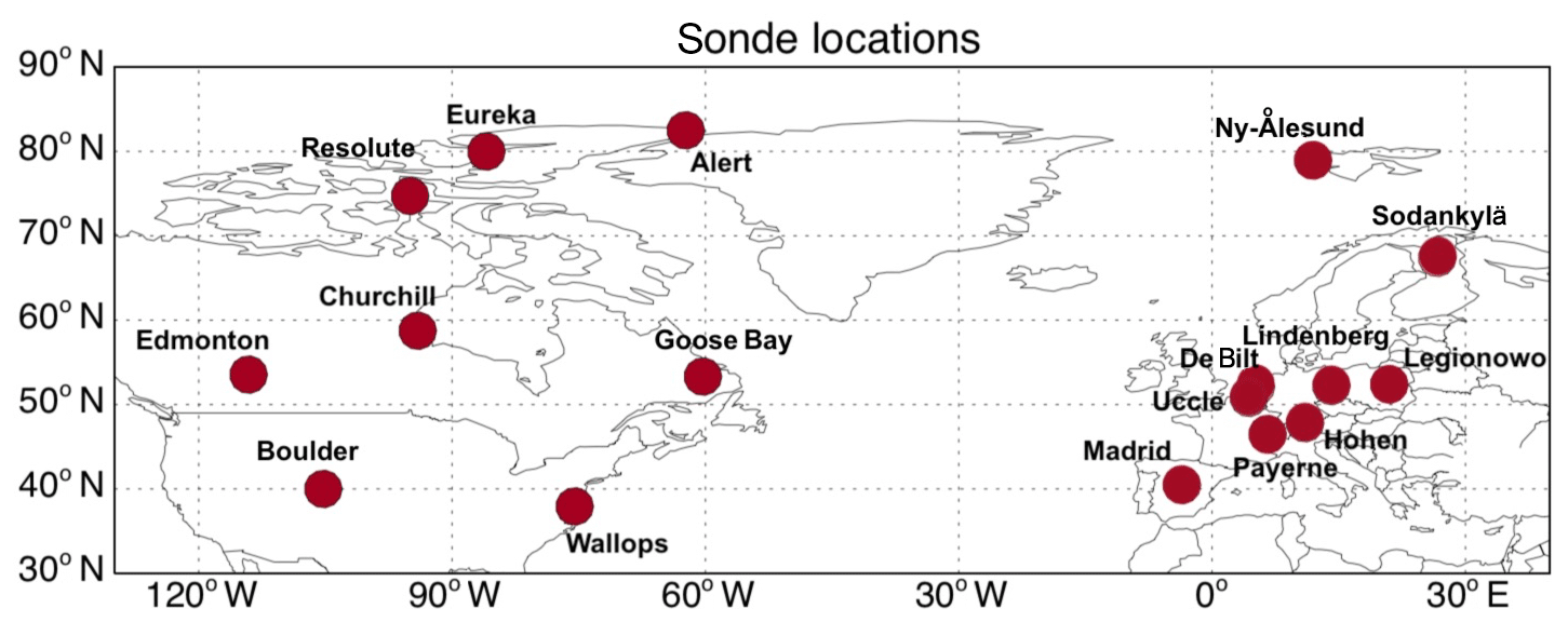
Figure 1Map of ozonesonde sites selected in this study.
Table 1The longitude, latitude, measurement time period and mean sampling frequency of the selected North American ozonesonde sites.
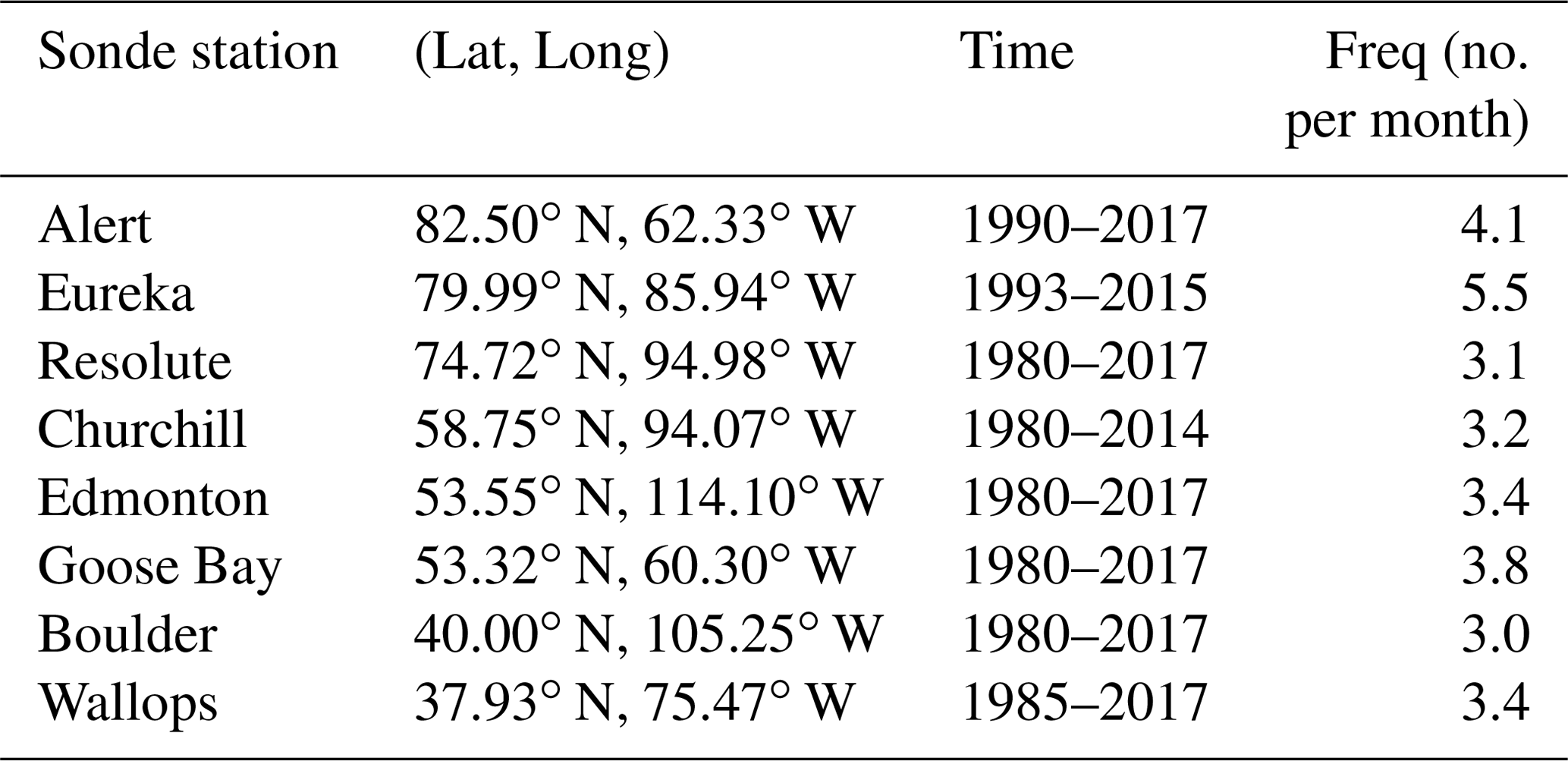
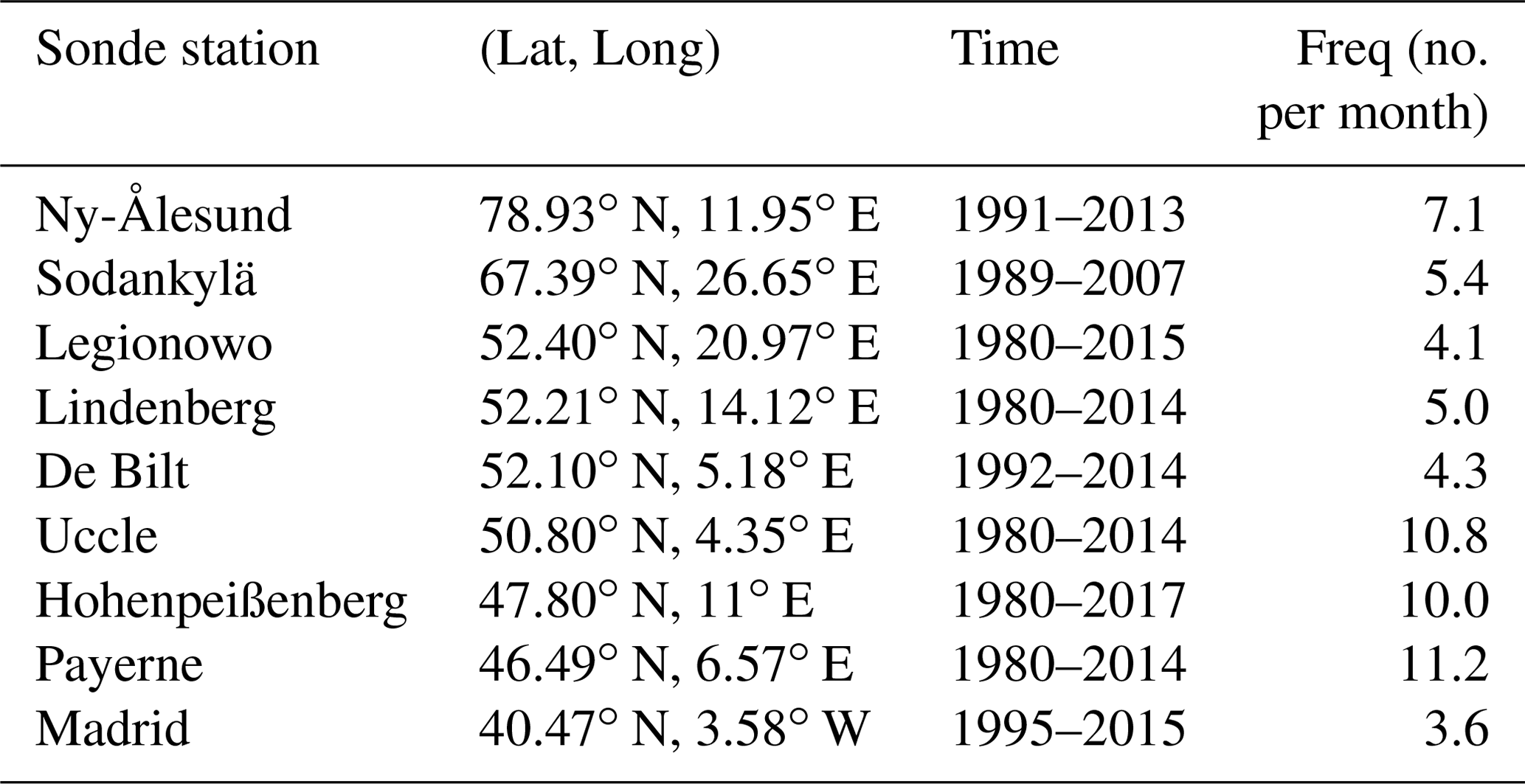
Table 2The longitude, latitude, measurement time period and mean sampling frequency of the selected European ozonesonde sites.
2.1 Ozonesondes
We select 17 ozonesonde sites, eight in North America and nine in Europe, all of which have a record of at least three profiles every month between 1990 and 2016 (Fig. 1 and Tables 1 and 2). The data are obtained from the World Ozone and Ultraviolet Radiation Data Centre (WOUDC; http://www.woudc.org, last access: 1 February 2020). Observations over most stations are obtained using electrochemical concentration cells (ECCs), which rely on the oxidation reaction of ozone with potassium iodide in solution (Komhyr et al., 1995). At Hohenpeißenberg, Germany, measurements are obtained using the Brewer–Mast instrument. The sonde ozone measurements have a vertical resolution of ∼150 m, with an accuracy of ±5 % in the troposphere (WMO, 2014).
2.2 MERRA2-GMI
We use a replay simulation (http://acd-ext.gsfc.nasa.gov/Projects/GEOSCCM/MERRA2GMI, last access: 1 February 2020) of the GEOSCCM with the Global Modeling Initiative (GMI) chemical mechanism (Duncan et al., 2007; Strahan et al., 2007) for gas chemistry, which includes a complete treatment of stratospheric and tropospheric chemistry, and the Goddard Chemistry Aerosol Radiation and Transport (GOCART) module (Chin et al., 2002; Colarco et al., 2010) for aerosols. The replay simulation follows the replay methodology as described in Orbe et al. (2017) and uses the RAs3 setting, which best represents overall transport. The model inputs the 3-hourly time-averaged output of MERRA-2 meteorology (U, V, T, pressure) and recomputes the analysis increments, which are used as a forcing to the meteorology at every time step over the 3 h replay interval. The replay simulation is run at a MERRA-2 native resolution of ∼50 km in the horizontal dimension and 72 vertical levels. This replay simulation is referred to as the “MERRA2-GMI” simulation.
The MERRA2-GMI simulation was run from 1980 to 2018. The emissions in this run include anthropogenic, biofuel, biomass burning and biogenic emissions. The values for fossil fuel and biofuel emissions are taken from the MACCity inventory (2011) until 2010 and then derived by following the Representative Concentration Pathway (RCP) 8.5 scenario after 2010. The MACCity anthropogenic emissions are derived by interpolating the Atmospheric Chemistry and Climate Model Intercomparison Project (ACCMIP) emissions (Lamarque et al., 2010) on a yearly basis between the base years 1990, 2000, 2005 and 2010. For the years 2005 and 2010, the interpolation follows the RCP 8.5 emission scenario. Biomass burning emissions are taken from the Global Fire Emissions Database (GFED) version 4s (Giglio et al., 2013) after 1997. Prior to 1997, biomass burning emissions are based on a GFED4s climatology with year-to-year variability imposed using regional scale factors derived from the Total Ozone Mapping Spectrometer (TOMS) aerosol index (Duncan et al., 2003). The simulation used the Model of Emissions of Gases and Aerosols from Nature (MEGAN) (Guenther et al., 2006) to simulate biogenic emissions, including isoprene, within the model. The lightning parameterization in the model (Allen et al., 2010) is constrained by the MERRA-2 detrended cumulative mass flux, with seasonal constraints from the Lightning Imaging Sensor (LIS)/Optical Transient Detector (OTD) v2.3 climatology (Cecil et al., 2014). Methane is specified using latitude and time-dependent surface observations from the NOAA Earth System Research Laboratory (ESRL) Global Monitoring Division (GMD) network (Dlugokencky et al., 2011). Our initial model evaluations suggest that the MERRA2-GMI ozone simulations are in good agreement with the means and variability of the total and tropospheric column ozone from satellite observations (Figs. S1 and S2 in the Supplement).
A StratO3 tracer is included in the model to diagnose the stratospheric ozone influence on the troposphere. StratO3 is set equal to simulated ozone in the stratosphere and is removed in the troposphere based on interannually varying monthly mean loss rates and surface deposition fluxes archived from a standard full chemistry simulation. StratO3 tracer is defined relative to a dynamically varying tropopause, which is derived from an artificial tracer, e90, introduced by Prather et al. (2011). The e90 tracer is set to a uniform mixing ratio (100 ppb) at the surface with a 90 d e-folding lifetime everywhere in the atmosphere. This lifetime is long enough for the tracer to be well mixed throughout the troposphere but short compared to the transport timescales in the stratosphere, resulting in sharp e90 tracer gradients across the tropopause. In our simulations, the e90 tropopause value is set to 90 ppb. Prather et al. (2011) shows that the e90 tropopause not only matches the other traditional definitions of the tropopause but also has the advantage of being able to capture complex features such as tropopause folds. Therefore, the e90 tropopause is optimal in effectively separating stratospheric from tropospheric air from a chemical composition perspective. The e90 tracer has been used in many studies of STE as an accurate tropopause definition and an ideal transport tracer in the upper troposphere and lower stratosphere (UTLS) (e.g., Hsu and Prather, 2014; Liu et al., 2016, 2017; Pan et al., 2016; Randel et al., 2016).
The MERRA2-GMI simulation has hourly output for ozone and 3-hourly output for StratO3 at each model level. When comparing to the ozonesonde measurements, the model outputs are sampled at the nearest grid point and launch time for each sonde.
3.1 Winter and spring ozone IAV in the lower stratosphere and troposphere over North American and European sites
Previous studies have shown that the relative contribution of stratospheric ozone to tropospheric ozone is greatest in the free troposphere during winter (e.g., Holton et al., 1995; Stohl et al., 2000; Skerlak et al., 2014, 2015) and at the surface during spring (e.g., Lin et al., 2012, 2015). In summer, the relative contribution of stratospheric ozone is low due to the increased chemical ozone production in the troposphere. Here, we focus on the winter (DJF) and spring (MAM) seasons to examine the interannual variations in the strength and vertical extent of stratospheric ozone impact on the tropospheric ozone.
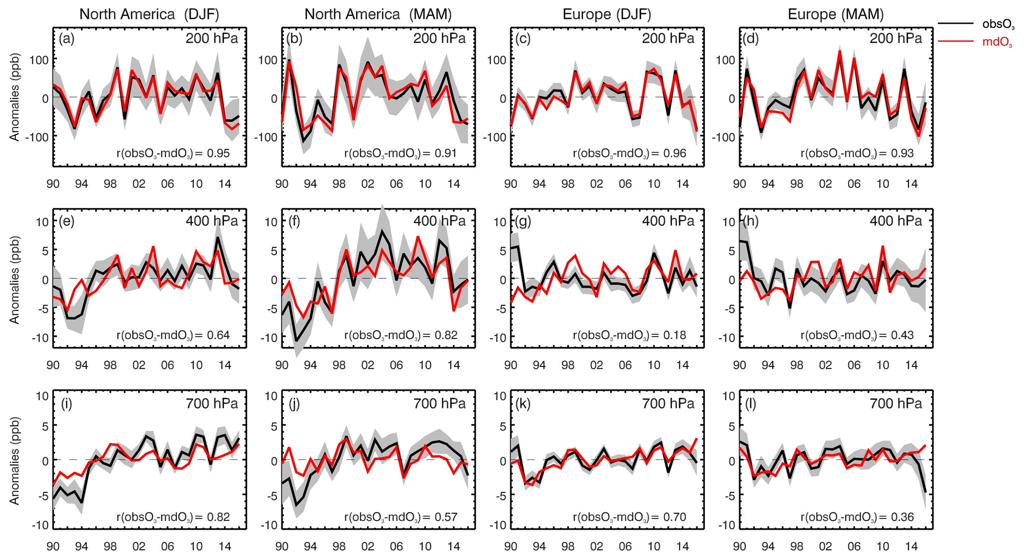
Figure 2Time series plots of observed (black) and simulated (red) ozone anomalies (unit: ppb) at 200 hPa (top), 400 hPa (middle) and 700 hPa (bottom) averaged from selected ozonesonde sites over North America and Europe in winter and spring seasons from 1990 to 2016. The anomalies are calculated by removing the seasonal mean averaged from 1990 to 2016. The shaded area represents the 95 % confidence interval (CI) of observed mean, which is calculated by multiplying the standard error of observations by 1.96.
Figure 2 compares the anomalies of modeled and ozonesonde measured ozone at 200, 400 and 700 hPa in the winter and spring seasons from 1990 to 2016 averaged over sites from North America and Europe. Anomaly at each site is calculated by removing the respective seasonal mean climatology from 1995 to 2016 and then averaged over all sites for each region (see the Supplement). The shaded area represents the 95 % confidence interval (CI) of the calculated mean from daily observations over all the selected stations. To quantify the magnitude of IAVs, we adopt the standard deviation (SD) of these ozone anomalies. We perform the standard statistical F test to assess the regional and seasonal differences in the ozone IAVs. The calculated standard deviations and F test statistics are shown in Tables S1 and S2.
At 200 hPa, the model reproduces well the observed IAV in both seasons over both regions (r≥0.91, Fig. 2a–d). There are no significant differences in the magnitude of ozone IAV between North America and Europe (Table S1). But over both regions, the ozone IAVs show significant seasonal differences with greater magnitude in spring than in winter (Table S2). Negative ozone anomalies occur in the early 1990s and at the end of the record from 2014 to 2016, while positive anomalies are obtained for most years between 1998 and 2013. The negative ozone anomalies during the period of 1992–1996 are consistent with the chemical and dynamical perturbations following the 15 June 1991 eruption of Mt. Pinatubo (Hadjinicolaou et al., 1997; Stenchikov et al., 2002; Rozanov et al., 2002). The negative ozone anomaly in 2015–2016 is associated with stratospheric circulation changes caused by the unusually warm ENSO event coinciding with a disrupted quasi-biennial oscillation (QBO) during that period (Tweedy et al., 2017; Diallo et al., 2018).
At 400 hPa, the model reproduces the IAV of the observations, with negative anomalies in the early 1990s and mostly positive anomalies thereafter. The observed negative ozone anomaly after the Mt. Pinatubo eruption has a maximum amplitude of 7 ppb (−13 % relative anomaly) in the winter of 1992–1994. The model underestimates the observed peak depletion in the winter of 1992, with the simulations falling outside the 95 % CI of the observations from 1992 to 1994 (Fig. 2e). In spring, the model reproduces well the timing of observed ozone depletion but again underestimates its amplitude (Fig. 2f). At 700 hPa, the observations from the North American sites show a similar negative ozone anomaly in 1992–1994 to that obtained at 200 and 400 hPa, with prevailing positive anomalies thereafter. The model results for the sign of the interannual variations are in relatively good agreement with observations but again underestimate the magnitudes of the negative anomalies in the early 1990s after the Mt. Pinatubo eruption.
Over European sites, the observed ozone IAV, excluding year 1990–1991, exhibits a similar pattern to the one at 200 hPa after 1991, although the minima after the Mt. Pinatubo eruption are not as pronounced as over North America (Fig. 2g–h). The maximum positive anomaly, observed in 1990–1991, is not reproduced by the model. The model–observation correlation coefficients increase significantly if we omit these 2 years (from 0.18 to 0.58 in the winter and from 0.43 to 0.58 in the spring). At 700 hPa, the model reproduces the magnitude of observed ozone depletion after the Mt. Pinatubo eruption. Unlike at 200 hPa, the differences in the magnitude of ozone anomalies between North America and Europe are significant at 400 and 700 hPa, with smaller ozone anomalies over European sites than over North American sites in both seasons (Table S1). The magnitude of ozone anomalies does not show significant seasonal difference between DJF and MAM, except over North America at 400 hPa (Table S2).
Table 3Variance explained (r2) of ozone between 200 and 400 hPa, 200 and 700 hPa in observations and simulations. The numbers in parentheses are variance explained for simulations.
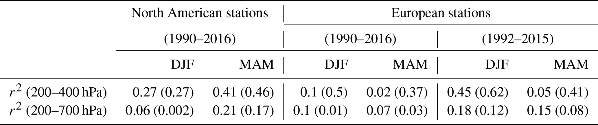
We use explained variance (square of correlation coefficient: r2) to determine the fraction of the ozone variance in the troposphere that can be attributed to the variance in stratospheric ozone. Table 3 shows the explained variances in the winter and spring ozone anomalies between 200 and 400 hPa, 200 and 700 hPa for the observations and simulations averaged over the North American and European stations. Both the model and observations suggest that about 27 % of North American ozone variations at 400 hPa are accounted for by changes at 200 hPa in the winter. The 200–400 hPa ozone relationship is higher in the spring (r2=0.4 in the observation and 0.46 in the simulation). Over Europe, the 200–400 hPa ozone relationship in the observations is relatively low (r2=0.1 in DJF and 0.02 in MAM), due to the phase shift of these two-time series during the first 2 years, where observed ozone anomalies are negative at 200 hPa but reach a maximum at 400 hPa. The explained variance increases to 0.45 after removing these 2 years in the winter but not that much in the spring (r2=0.05). High correlations of the ozone anomalies between 200 hPa and 400 hPa are seen in the model in both seasons. The highest relationship between 200 and 700 hPa is found over the North American sites in the spring with r2=0.21 and 0.17, respectively, in the observation and simulation, which is consistent with the previous findings of the deep STE hotspots along western US in the spring season (Lin et al., 2012; Skerlak et al., 2014; Langford et al., 2015).
The correlations between the stratosphere and troposphere IAV in both observations and model simulations suggest a potential impact of stratospheric ozone on tropospheric ozone variations. Previous studies have found high correlations between ozone in the lower stratosphere with that in the middle and lower troposphere, with the largest effects in late winter and spring. Correlation does not necessarily mean causality, and to date, model investigations of this correlation (Terao et al., 2008; Hess and Zbinden, 2013) have not used a model with both stratospheric and tropospheric chemistry and up-to-date stratospheric circulation. The MERRA2-GMI simulation has both of these attributes, detailed dynamic diagnostics and StratO3 as described in Sect. 2.2. In the next section, we use the StratO3 tracer to examine the contribution of stratospheric ozone to the IAV of tropospheric ozone, as a function of altitude, season and location. We will also use diagnostics from the model to explore the influence of transport on the stratospheric ozone contribution to the tropospheric ozone and its IAV.
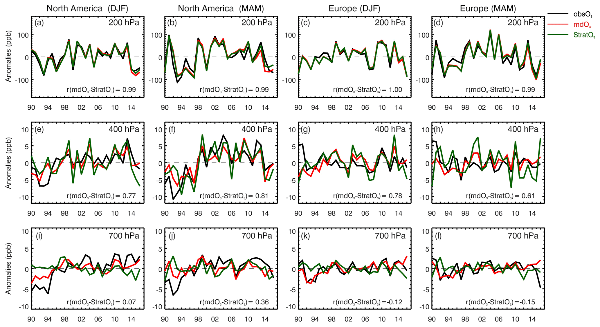
Figure 3Similar to Fig. 2 but adding the simulated StratO3 anomalies (green). The correlation coefficients between simulated ozone and StratO3 are shown in text.
3.2 Impact of stratospheric ozone on tropospheric ozone IAV
Figure 3 shows the same comparison between the observed (black lines) and simulated ozone (red lines) anomalies as in Fig. 2 but adding the anomalies of simulated StratO3 (green lines). As expected, the StratO3 anomalies at 200 hPa are almost identical to the simulated ozone anomalies, since most measurements are in the stratosphere at this level.
The variability in the amount of tropospheric ozone that was transported from the stratosphere as inferred by StratO3 is due to both the variability in the lower stratospheric ozone reservoir and the variability in the net downward mass flux (Albers et al., 2018). These two variabilities may either cancel or reinforce each other, depending on their relative phases. At 400 hPa, over the North American stations, the minimum and maximum of StratO3 tracer is highly correlated with the minimum and maximum of simulated ozone. The IAV of StratO3 explains more than 60 % of simulated ozone variations (Fig. 3e, f; r=0.77 in DJF and 0.81 in MAM), suggesting that the changes in stratospheric ozone input strongly impact the simulated ozone IAV in the upper troposphere. The correlation between StratO3 and observed ozone is slightly lower (0.44) than that with simulated ozone in DJF over North America. The decreased correlation is mainly due to the model–observation discrepancy between 1992–1994. The sondes at 400 hPa show a similar ozone depletion through 1992–1994 as seen at 200 hPa after the Mt. Pinatubo eruption, while the model shows an ozone increase after 1992 through 1994, which is driven by changes in the stratospheric ozone contribution to the modeled ozone (Fig. 3e). This suggests that the impact of the negative anomalies of stratospheric ozone (200 hPa) may be counterbalanced by an increase in downward mass flux from the stratosphere, thus leading to the model underestimation of the negative anomaly in observations at 400 hPa. In MAM, the StratO3-measured O3 correlation is high (0.74) over North America. Over European sites, a similar correlation is observed between simulated ozone and StratO3 at 400 hPa in the winter (r=0.78), with a slightly smaller value in the spring (r=0.61). The correlation decreases when comparing StratO3 to the observed ozone, mainly because of the model–observation discrepancy during the first 2 years. Omitting the first 2 years gives a fair correlation between StratO3 and observed ozone (0.66 in DJF and 0.34 in MAM). The fair-to-good correlations between StratO3 and observed ozone indicate a significant impact of stratospheric ozone on the tropospheric ozone variations at 400 hPa over both North America and Europe..
Figure 3i–l compare the simulated StratO3 anomalies to the observed and simulated ozone anomalies at 700 hPa over North American and European ozonesonde sites during winter and spring. Over North America, the observed ozone anomalies stay low in the early 1990s and increase thereafter in both seasons, which is underestimated in the model. In the winter, StratO3 anomalies decrease slightly in contrast to increases in both observed and simulated ozone anomalies. The winter StratO3–O3 correlation is ∼0. In spring, both observed and simulated ozone exhibit similar IAV, which agree with the phase of the StratO3 anomalies after the Pinatubo period (1991–1995). The StratO3–O3 correlation increases from 0.07 to 0.33 in winter and from 0.36 to 0.58 in spring from 1996 to 2016.
Over North America, our model results are in good agreement with the observed IAV at all levels except right after the Mt. Pinatubo eruption. The model only reproduces about half of the observed tropospheric depletion over North America. As discussed above, this could be due to an excessive mass flux from the stratosphere in the MERRA-2 analysis during this period. Model results are in better agreement with the magnitude of observed ozone depletion after the Mt. Pinatubo eruption in the middle and lower troposphere over Europe. There is no significant relationship between StratO3 and simulated ozone at 700 hPa. This is expected since the impact of stratospheric ozone decreases, and the impact of ozone production from its precursors becomes more important at lower altitudes. In summary, our model analysis identifies differences in the strength and vertical extent of stratospheric ozone impact on the tropospheric ozone IAV between North America and Europe. Over North America, the StratO3 IAV has a significant impact on the tropospheric ozone IAV from the upper to lower troposphere and explains 60 % and 66 % of the simulated ozone IAV at 400 hPa and 11 % and 34 % at 700 hPa in winter and spring, respectively, after 1995. Over Europe, the influence is limited to the middle to upper troposphere and becomes much less at 700 hPa.
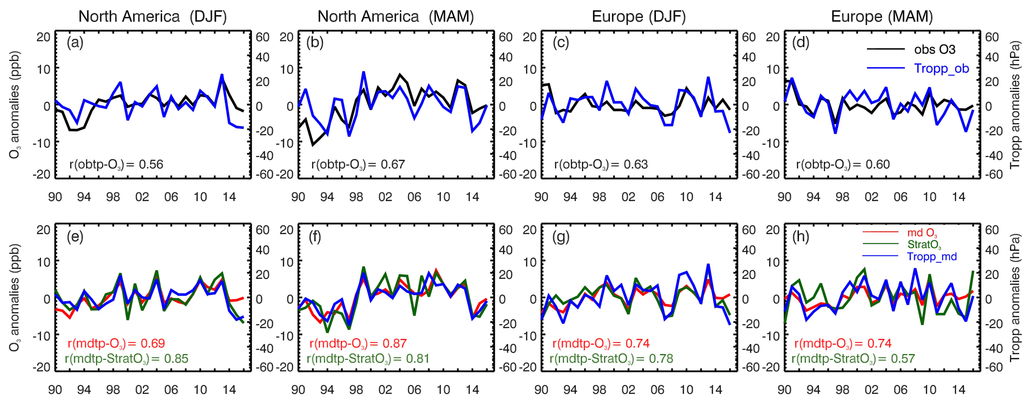
Figure 4(a–d) Time series of the observed ozone mixing ratio anomalies at 400 hPa and the tropopause pressures derived from observed ozone profiles averaged over the North American and European sites in winter and spring. Their correlation coefficients are shown in black text. (e–h) Time series of the simulated ozone and StratO3 anomalies at 400 hPa with the tropopause pressures derived from simulated ozone profiles, with the respective correlation coefficients shown in red and green text.
The differences in the stratospheric ozone impact between North America and Europe are likely due to variations in the net downward flux associated with planetary-scale waves. Previous studies have suggested that the IAV of the STE mass flux is likely correlated to changes in the tropopause height (e.g., Gettelman et al., 2011). Figure 4a–d show the comparison of the observed ozone mixing ratio anomalies at 400 hPa and the tropopause pressures derived from the observed ozone profiles following the criteria in vertical gradient and ozone mixing ratio given by Browell et al. (1996). The tropopause pressure was estimated to be at the pressure where a linear regression line passing through the lower stratospheric ozone profile (150–400 ppb, lower than 100 hPa) intersects with the 100 ppb ozone level. Figure 4e–h compare the simulated ozone and StratO3 anomalies at 400 hPa with the tropopause pressures derived from simulated ozone profiles following the same criteria as for the observations. As expected, the IAV of ozone and StratO3 positively correlates with that of the derived tropopause pressure (anticorrelates with the tropopause height) in both model and observation. In general, during years with a lower tropopause, stratospheric ozone influence at 400 hPa increases and results in a positive ozone anomaly. During years with a higher tropopause, decreased stratospheric ozone influence leads to a negative ozone anomaly at 400 hPa.
The above high correlations between the IAV of tropopause pressure and StratO3 raise the question of what dynamical conditions control the higher/lower tropopause pressures, STE mass fluxes and the subsequent impact of stratospheric ozone on tropospheric ozone. These questions are particularly important if these dynamical conditions change in the future as a result of climate change. In the next section, we rely on the model's 3-D dynamical diagnostics, including air mass flux and horizontal wind patterns, to examine both the vertical and horizontal transport influence of the stratospheric ozone contribution on the tropospheric ozone and its IAV. We also examine the longitudinal difference in the model's dynamics to explain the identified differences in the stratospheric ozone impact between North America and Europe.
4.1 Case study of 3-D dynamic characteristics
Planetary-scale Rossby waves, superimposed on the mean westerly zonal flow, are the dominant dynamical variability over northern midlatitudes in winter and spring. Troughs occur where the flow moves equatorward. Tongues of stratospheric polar air extend equatorward associated with frequent STE processes. Ridges occur where the flow moves poleward, bringing in warm tropospheric air. The Northern Hemisphere is typically encircled by several of these waves, with troughs (ridges) likely occurring over eastern (western) continental edges (e.g.,Thorncroft et al., 1993). Homeyer and Bowman (2013) have shown that a Rossby wave in the upper troposphere can affect the flow in the lower levels and plays an important role in the meridional transport of both tropical and subtropical air masses. Ozone transport associated with these wave disturbances are responsible for a large fraction of ozone temporal and spatial variability in winter and spring (e.g., Kinnersley and Tung, 1998; McCormack et al., 1998; Lozitsky et al., 2011; Zhang et al., 2015).
In this section, we examine the linkage of the vertical and horizontal transport to the stratospheric ozone contribution in the troposphere using the model's 3-D air mass flux and horizontal winds. Our analysis focuses on the year 1993, when there is a major discrepancy with the observations at 400 hPa as shown in Fig. 3.
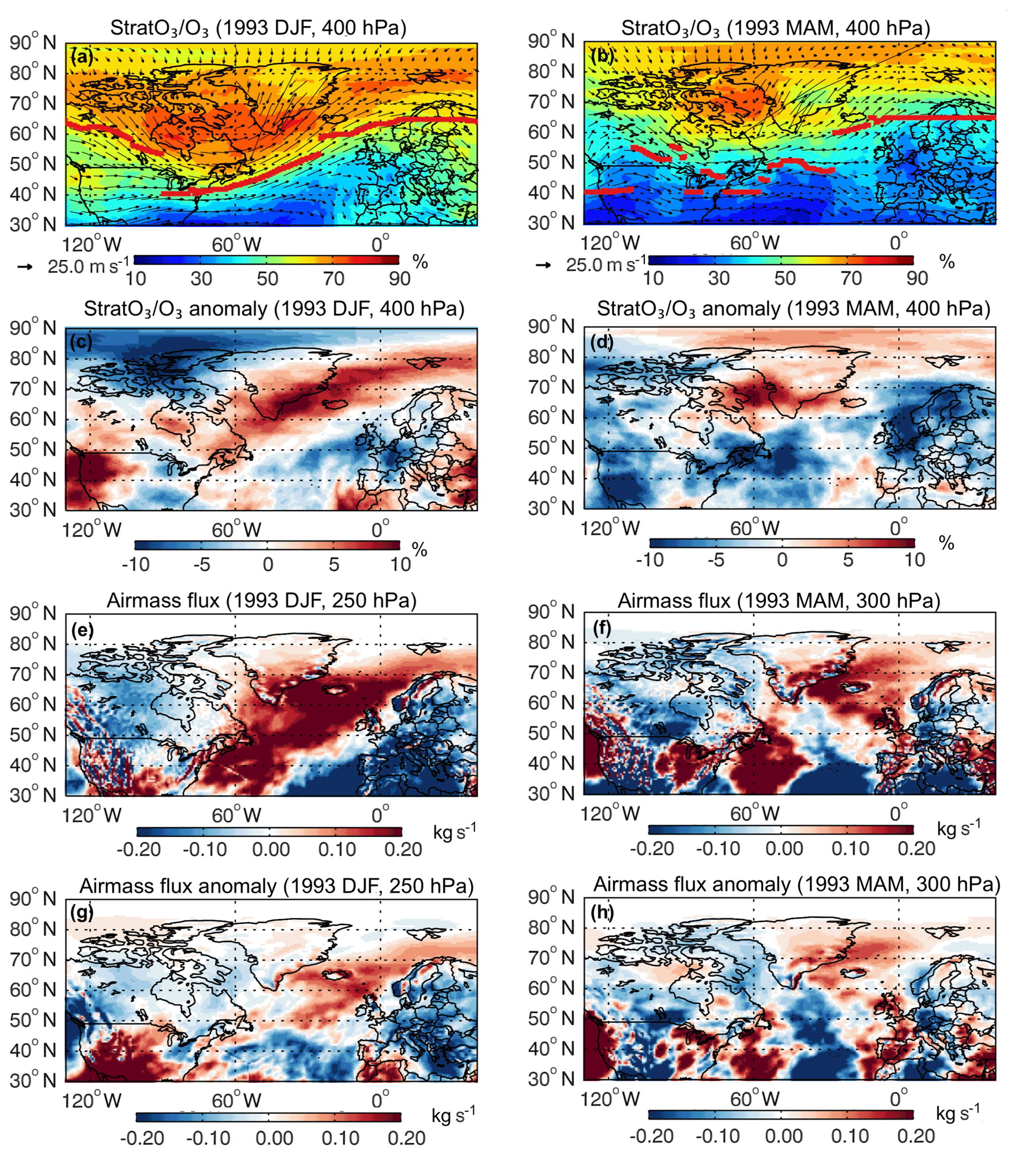
Figure 5Spatial maps of simulated (a, b) StratO3∕O3 ratio and (c, d) its anomaly at 400 hPa and (e, f) air mass flux and (g, h) its anomaly at the seasonal mean tropopause pressure in the winter (left) and spring (right) of 1993. The seasonal mean tropopause pressure in the model averaged from 30 to 80∘ N is around 250 hPa in winter and around 300 hPa in spring. Thin black arrows in first row represent the prevailing wind pattern at 400 hPa. Thick red lines indicate the jet locations, where the strongest winds are.
Figure 5 illustrates the relationship of the StratO3∕O3 ratio at 400 hPa to the horizontal winds at 400 hPa and the vertical air mass flux near the seasonal mean tropopause pressure in the year 1993. The seasonal mean tropopause pressure in the model averaged from 30 to 80∘ N is around 250 hPa in winter and around 300 hPa in spring. Because of the different tropopause heights, different pressure levels are shown in the figures. The vertical air mass flux is calculated by multiplying omega (dp ∕ dt; units: pa s−1) with the density of air. The sign of calculated air mass flux is reversed so that positive values represent upward fluxes; negative values represent downward fluxes. Figure 5a and b show the simulated StratO3∕O3 ratio in the winter and spring of 1993; prevailing wind patterns at 400 hPa are superimposed on this ratio. The jet, the location of maximum winds, is indicated by thick red lines. Figure 5c and d show the anomalies of simulated StratO3∕O3. Figure 5e and h show the vertical air mass flux around the tropopause pressure (blue color represents the downward motion, and red color represents the upward motion near the tropopause) and their anomalies (blue color represents an increase in downward flux or a decrease in upward flux; red color represents a decrease in downward flux or an increase in upward flux around the tropopause).
In the winter of 1993, the jet at 400 hPa exhibited a typical wave pattern, with a trough over eastern North America and ridges over western North America and western Europe (Fig. 5a). Strong northwesterly winds prevailed north of 50∘ N over western North America. They converged with the westerlies around 45∘ N in eastern North America. The winds then changed direction to southeasterly and flowed into the North Atlantic and Europe, bringing warmer tropospheric low ozone air into western Europe (Fig. 5a). The maps of the air mass flux and its anomalies (Fig. 5e and g) suggest that North America between 50 and 70∘ N was dominated by more vigorous downward mass fluxes of stratospheric air. Meanwhile, the northwesterly winds brought ozone-rich air from high latitudes, resulting in a positive anomaly of stratospheric ozone influence at 400 hPa (Fig. 5c). Although the lower stratospheric ozone level decreased significantly in the winter of 1993 due to the Pinatubo eruption (Fig. 2), the enhanced downward mass fluxes across the tropopause in the model counteracted the depletion and led to a positive ozone anomaly at 400 hPa over North America between 50 and 70∘ N (Fig. S3). Over the high latitudes (>70∘ N), where there is less dynamic perturbation (including both vertical and horizontal transport), the stratospheric ozone contribution at 400 hPa was largely driven by the depletion of the ozone concentration in the lower stratosphere and showed a strong negative anomaly in 1993 (Fig. 5c). Most of the European region was covered by the increased downward air mass flux near the tropopause in the winter of 1993. However, a negative anomaly of the StratO3 contribution at 400 hPa was seen over western Europe. It is likely that the combined negative effects of the ozone depletion in the lower stratosphere and the downwind of the warmer tropospheric low ozone air from the subtropical North Atlantic Ocean exceeded the positive effect of the increased downward air mass flux over this region.
In the spring of 1993, regions with maximum StratO3∕O3 at 400 hPa were located further north compared to those in the winter and centered around the northern part of the Labrador Sea. Southwesterly wind prevailed south of 65∘ N over western North America, bringing in low-StratO3 oceanic air from the subtropics. The winds changed direction to northwesterly around 120∘ W and 65∘ N and flowed westerly around the Hudson Bay until reaching the west coast of Europe. The winds then bifurcated into two branches: one passed by the northern side of Europe and the other flowed around the southern side of Europe. In North America south of 50∘ N, there were three cells with increased upward air mass fluxes near the tropopause ranging from 110 to 50∘ W (Fig. 5f, h). Regions downwind of these cells exhibited a negative anomaly of stratospheric ozone contribution at 400 hPa (western North America, eastern North America from the Great Lakes and west North Atlantic, Fig. 5d). Over Hudson Bay and the central US, the increased downward mass flux near the tropopause contributed to the slightly positive anomaly of the stratospheric ozone contribution at 400 hPa. Over the north and west of Europe, the combined negative effects from the increased upward mass flux across the tropopause (Fig. 5f, h) as well as downwind of the westerly flows with low stratospheric ozone (Fig. 5b) led to strong negative anomalies in the stratospheric ozone contribution at 400 hPa.
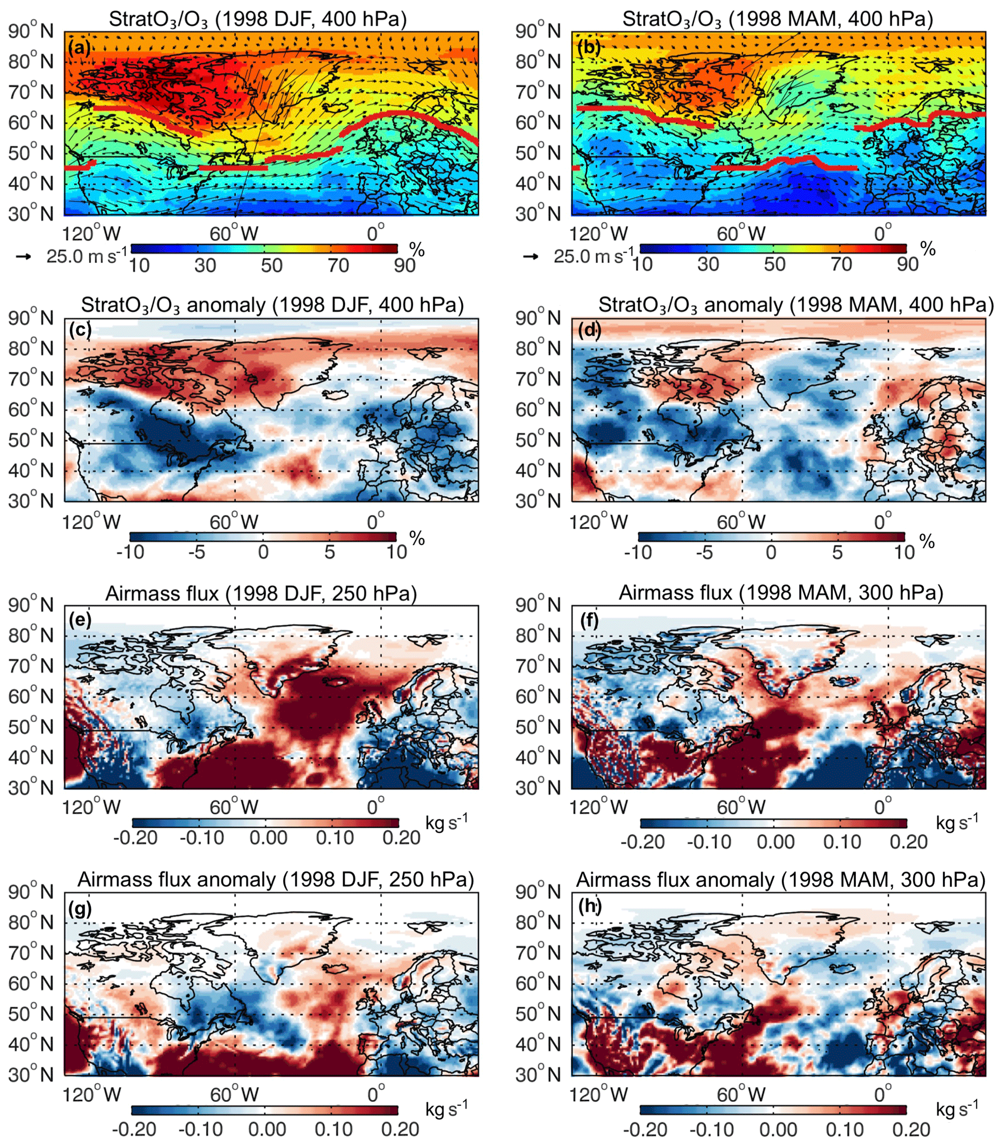
Figure 6Similar to Fig. 5 but for the year 1998.
Figure 6 shows a similar analysis as Fig. 5, except for 1998, when stratospheric ozone levels have recovered from the Mt. Pinatubo eruption and reached a regional maximum (Fig. 2). In the winter of 1998, a poleward shift of the jet occurred over most of North America. The jet location as well as the regions with the maximum StratO3∕O3 ratio moved to the north by about 7∘ compared to the winter of 1993 (Fig. 6a). With the poleward shift of the jet, the StratO3∕O3 anomaly exhibited a negative (positive) maximum along the equatorward (poleward) side of the jet. Southwesterly winds prevailed over regions equatorward of the jet at 400 hPa, bringing in tropical oceanic low ozone air to North America. Around the tropopause, there were increased upward air mass fluxes along the west coast of North America and decreased downward air mass fluxes over western and central North America. Therefore, although there was an increase in the stratospheric ozone concentration in 1998, the wind patterns in the troposphere and the vertical mass flux around the tropopause associated with the northward shift of the jet system caused a less favorable transport of stratospheric ozone into troposphere. This resulted in a negative anomaly of StratO3∕O3 at 400 hPa over most of North America. In the spring of 1998, a similar poleward shift of the jet occurred over North America as that in the winter, with a negative StratO3∕O3 anomaly over most of North America north of 45∘ N (Fig. 6b, d).
Our analysis suggests that significant interannual variations exist in both the regional wind patterns associated with the westerlies waves and the strength of downward air mass fluxes across the tropopause. The IAV of stratospheric ozone influence in the troposphere reflects a combined effect of the IAV in the 3-D dynamics as well as that in the lower stratospheric ozone concentration, which may either oppose or reinforce each other.
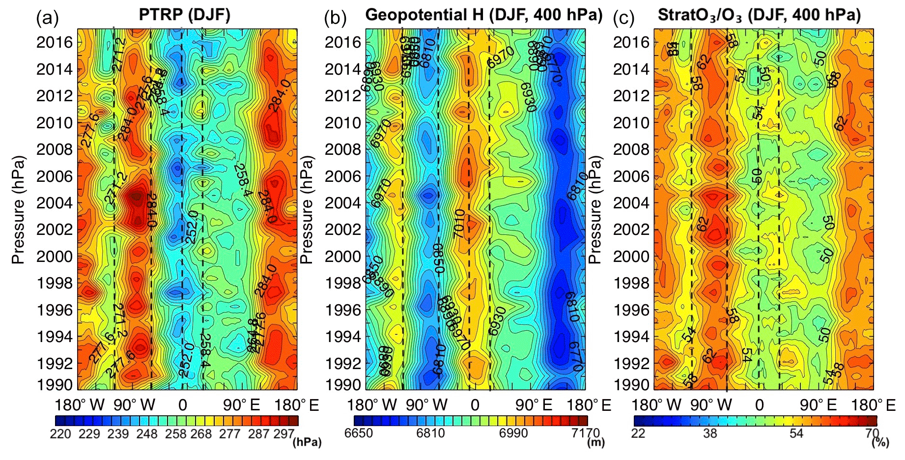
Figure 7Latitudinal average between 30 and 80∘ N of (a) the tropopause pressure, (b) the geopotential height at 400 hPa and (c) the StratO3∕O3 ratio at 400 hPa along each longitude from 180∘ W to 180∘ E from 1990 to 2016 in winter (DJF). Dashed lines indicate the longitudinal range for the North American region (120–60∘ W) and the European region (10∘ W–26∘ E).
4.2 Longitudinal difference in stratospheric ozone influence
Our analysis based on data and model sampled at sonde sites identified differences in the strength and vertical extent of stratospheric ozone impact on tropospheric ozone IAV between North America and Europe. Over North American sites, a significant impact of the StratO3 IAV on tropospheric ozone extends to the lower troposphere. Over European sites, the influence is limited to the middle to upper troposphere. In this section, we examine whether the longitudinal differences seen over the ozonesonde sites are a large-scale phenomenon, by extending our analysis to a broader spatial domain. Figures 7 and 8 show the latitudinal average (30 to 80∘ N) of tropopause pressure, geopotential height at 400 hPa and the StratO3∕O3 ratio at 400 hPa at each longitude from 180∘ W to 180∘ E from 1990 to 2016 in winter and spring. The geopotential heights and tropopause pressure are good diagnostics of large-scale circulation patterns. All of them show strong longitudinal difference between North America (120–60∘ W) and Europe (10∘ W–26∘ E), with lower geopotential height, higher tropopause pressure (lower tropopause height) and greater stratospheric ozone contribution over North America than over Europe. The longitudinal gradients between North America and Europe are slightly weaker in spring than in winter. The spatial map of StratO3∕O3 climatology at 400 hPa averaged from 1990 to 2016 suggests that the longitudinal difference is persistent over most of the mid-high latitudes (Fig. S4) and is closely related to the wavelike pattern in jets. The climatology of jet meanders to the south over central and eastern North America and brings in cold polar air with more stratospheric subsidence. The jet moves to the north over Europe and brings in warm air with less stratospheric ozone influence. Skerlak et al. (2014) identified the deep STE hotspots along western North America using the ERA-Interim reanalysis data set from the European Centre for Medium-Range Weather Forecasts (ECMWF) from 1979 to 2011. Therefore, over North America, the stratospheric subsidence inside the polar vortex as well as deep stratospheric intrusion events results in a deeper and greater stratospheric ozone influence on the tropospheric ozone than over Europe.
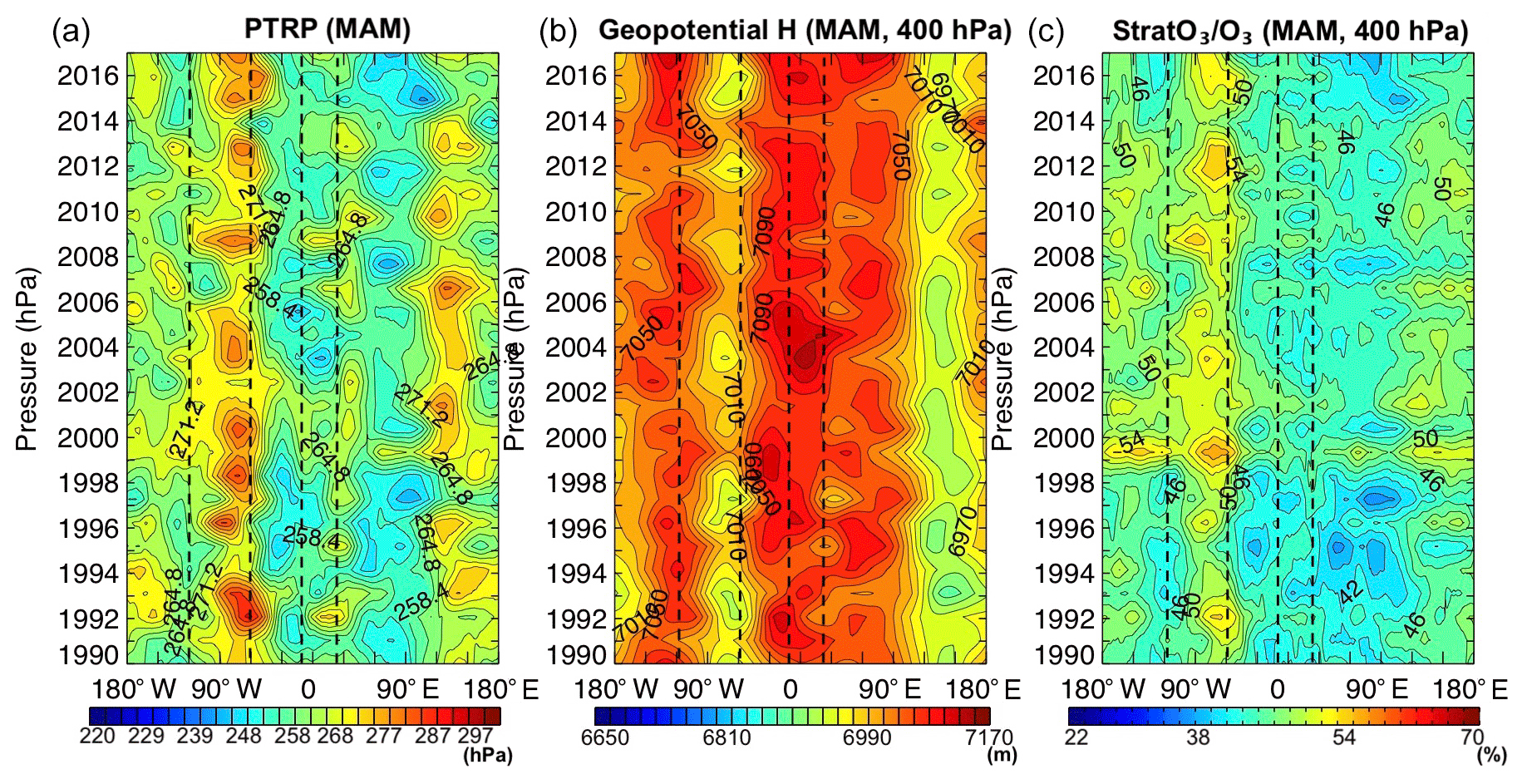
Figure 8Latitudinal average between 30 and 80∘ N of (a) the tropopause pressure, (b) the geopotential height at 400 hPa and (c) the StratO3∕O3 ratio at 400 hPa along each longitude from 180∘ W to 180∘ E from 1990 to 2016 in spring (MAM). Dashed lines indicate the longitudinal range for the North American region (120–60∘ W) and the European region (10∘ W–26∘ E).
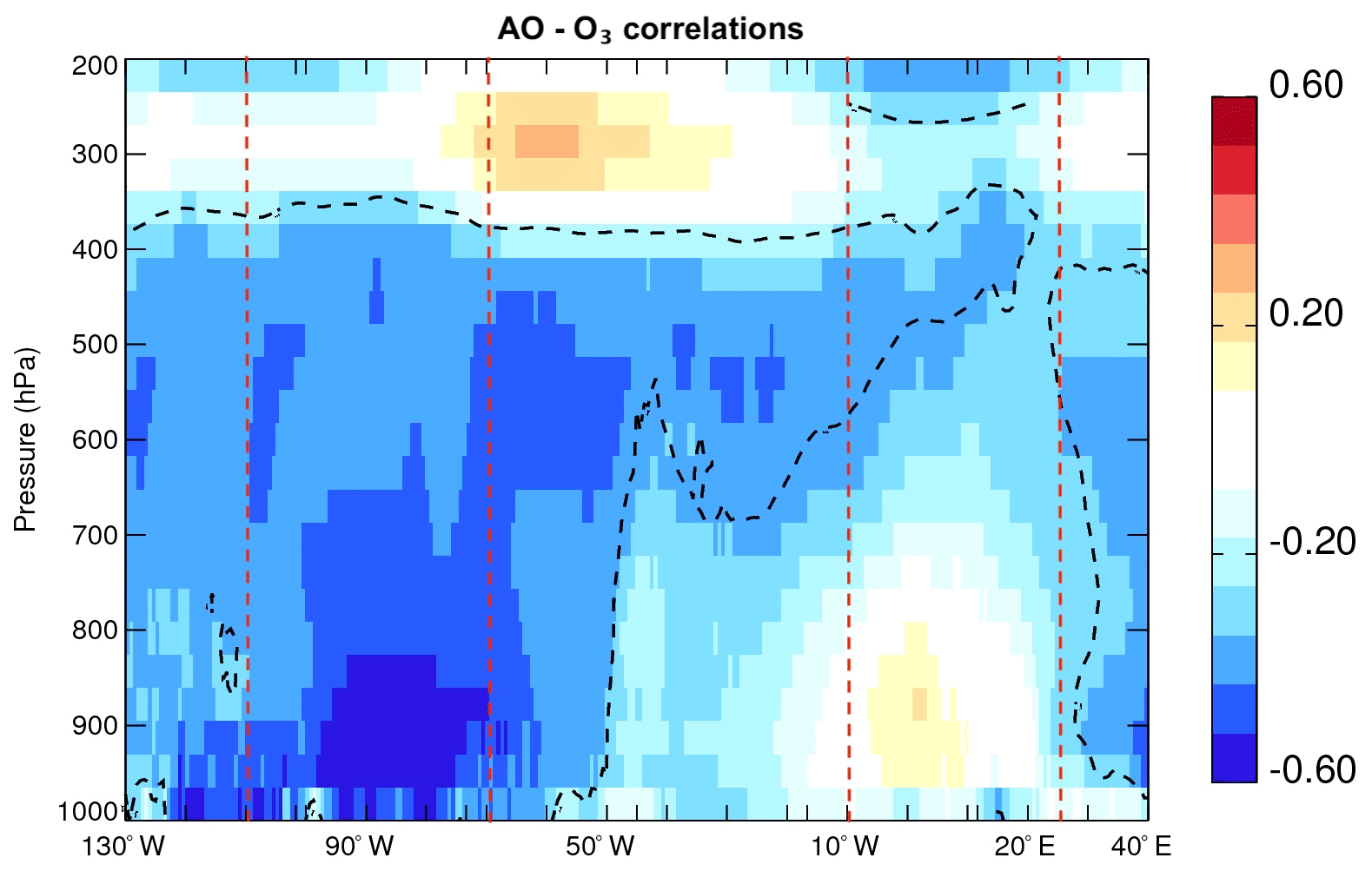
Figure 9Longitudinal variations in correlation profiles (r) between AO index and simulated ozone averaged over 30 and 80∘ N in DJF from 1000 to 200 hPa. Correlations inside black dashed lines are statistically significant (df=25; p<0.05). Red dashed lines indicate the longitudinal range for the North American region (120–60∘ W) and the European region (10∘ W–26∘ E).
A modulating factor in the IAV is the Artic Oscillation (AO) – the primary mode of dynamical IAV in the troposphere during winter. Several studies have examined the mechanism for downward transport from the stratosphere to the troposphere and attributed changes in the strength of lower-stratospheric polar vortex to AO anomalies at the surface, with a positive AO phase linked to a more isolated and stronger polar vortex (Ambaum and Hoskins, 2002; Perlwitz and Harnik, 2003) and lower tropopause heights. Lamarque and Hess (2004) found that the AO explains up to 50 % of the IAV in tropospheric ozone over North America in January–March but did not find any significant correlation in European sonde data, with similar results from the Model for OZone And Related chemical Tracers (MOZART) model. They argued that the correlation may be caused by the influence of the AO on its modulation of STE as well as transport of ozone and its precursors. Kivi et al. (2007) found that changes in the AO explained most of the tropospheric ozone trends in January–April, based on analysis of Arctic ozonesonde data. Figure 9 shows the longitudinal variations in simulated ozone and AO correlation profiles averaged over 30 and 80∘ N from 1000 to 200 hPa. Over North America (120 to 60∘ W), the correlation between simulated ozone and the AO index is negative and stays low above 400 hPa. The anticorrelation increases with increased pressure and reaches its maximum near the surface around 90∘ W. The anticorrelation averaged over Europe (10∘ W–26∘ E) stays low above 400 hPa, increases slightly from 400 to 700 hPa, then decreases sharply near the surface. This is similar to the correlations obtained from the ozonesonde profiles (Fig. S5). The similarity of correlation patterns over sonde sites and their surrounding broader regions indicates that the AO-related stratospheric subsidence is a large-scale phenomenon.
In this study we used ozone and stratospheric ozone tracer simulations from MERRA-2 GMI and observations from ozonesondes to investigate the interannual variations and vertical extents of the stratospheric ozone impact on tropospheric ozone. Our work focuses on the winter and spring seasons over North America and Europe.
The model reproduces the observed interannual variations in tropospheric ozone over North America except for the Pinatubo period from 1991 to 1995. The ozonesonde data show a negative ozone anomaly in 1992–1994 following the Pinatubo eruption, with recovery thereafter. However, the simulated anomaly is about half the magnitude of the observed tropospheric ozone depletion. Over European regions, ozonesonde measurements show a similar but weaker ozone depletion, which was fully reproduced by the model. We use a stratospheric ozone tracer to gauge the impact of stratospheric ozone variations in different regions of the troposphere. Our results based on the stratospheric ozone tracer suggest that the influence of the stratospheric IAV is significant in the upper to lower troposphere over North America, while over Europe, the stratospheric influence is limited to the middle to upper troposphere. Our analysis of the MERRA2 assimilated fields shows strong longitudinal variations in meteorological parameters over Northern Hemisphere mid-high latitudes, with lower tropopause height and lower geopotential height over North America than over Europe. These variations associated with the relevant variations in the location of tropospheric jet flows are responsible for the longitudinal change in the stratospheric ozone influence. The increase in frequency in stratospheric folds near the jets and the strong winter subsidence inside the polar vortex lead to stronger stratospheric impact over North America than over Europe.
We examined the linkages of horizontal and vertical dynamical structures in the lower stratosphere to the contributions of stratospheric ozone in the upper and middle troposphere. Our analysis suggests that the IAV of wave disturbances of the westerlies likely affect the IAV of the prevailing wind patterns as well as the strength of STE flux. The IAV of stratospheric ozone influence in the troposphere reflects a combined effect of the changes in the lower stratospheric ozone concentration and in the 3-D dynamics, which may either oppose or reinforce each other, depending on their relative phases.
Our analysis provides an in-depth understanding of how dynamics influences the ozone redistribution in the troposphere and reveals deficiencies in the model's transport. The observed ozone at 400 hPa over the North American sites show a similar ozone depletion as that at 200 hPa after the Mt. Pinatubo eruption, while the model only reproduces about half the magnitude of the observed ozone depletion at 400 hPa. The effect of lower stratospheric ozone concentration seems masked by the increased stratospheric-tropospheric flux, indicated by increased tropopause pressure accompanied by a stronger downward air mass flux in the model, especially between 50 and 70∘ N. Therefore, the model underestimation of the observed ozone depletion after the Mt. Pinatubo eruption over North America in the lower troposphere could be due to the STE flux being too strong in the model for this region during that period. The deficiencies in the model's transport might come from the limitations of the input MERRA-2 meteorological fields during early 1990s. The assimilated MERRA-2 meteorological fields are significantly improved after the year 1998 when many higher-resolution meteorological observations are included in the assimilation (Bosilovich et al., 2015; Stauffer et al., 2019). Apart from the input meteorological fields, the discrepancies might be also due to the replay configuration used in the model. Orbe et al. (2017) showed that small differences are seen in stratosphere–troposphere exchange between the GMI-CTM and a replay simulation constrained with the same meteorological fields. In spite of the weaker response in the model, the general agreement between the model and observations and the correlation between StratO3 and measurements indicate a significant impact of stratospheric ozone variations on tropospheric ozone.
All data used for this article can be obtained by contacting Junhua Liu (junhua.liu@nasa.gov).
The supplement related to this article is available online at: https://doi.org/10.5194/acp-20-6417-2020-supplement.
JL performed the data and model analysis and wrote the paper; JL and JMR conceived and planned the project and participated in the numerous scientific discussions. LDO performed and provided the MERRA2-GMI simulation. ARD provided insights on interpolation of model and data comparison. LDO and MAO helped on dynamical analysis of model simulations and interpolation of the findings. LH prepared ozonesonde data. All authors provided critical feedback and helped shape the research, analysis and paper.
The authors declare that they have no conflict of interest.
The first author gratefully acknowledges the financial support by NASA's Atmospheric Chemistry Modeling and Analysis Program (ACMAP). We thank the World Ozone and Ultraviolet Radiation Data Centre and the SHADOZ program for making the routine sonde data accessible. We gratefully acknowledge Jerry R. Ziemke from NASA for providing the OMI/MLS TCO data and Stacey M. Frith from NASA for providing SBUV total ozone column data. Work was performed under contract with NASA at Goddard. We thank Clara Orbe for her helpful comments on the model's replay configuration. Computer resources for the MERRA-2 GMI simulation were provided by the NASA Center for Climate Simulation. We thank the editor and the reviewers for their helpful comments and suggestions to improve this paper.
This research has been supported by the NASA Aura Science Team and ACMAP (2016) (grant no. NNH16ZDA001N-ACMAP/NNX17AG58G).
This paper was edited by Andreas Engel and reviewed by three anonymous referees.
Akritidis, D., Katragkou, E., Zanis, P., Pytharoulis, I., Melas, D., Flemming, J., Inness, A., Clark, H., Plu, M., and Eskes, H.: A deep stratosphere-to-troposphere ozone transport event over Europe simulated in CAMS global and regional forecast systems: analysis and evaluation, Atmos. Chem. Phys., 18, 15515–15534, https://doi.org/10.5194/acp-18-15515-2018, 2018.
Albers, J. R., Perlwitz, J., Butler, A. H., Birner, T., Kiladis, G. N., Lawrence, Z. D., Manney, G. L., Langford, A. O., and Dias, J.: Mechanisms Governing Interannual Variability of Stratosphere-to-Troposphere Ozone Transport, J. Geophys. Res.-Atmos., 123, 234–260, https://doi.org/10.1002/2017jd026890, 2018.
Allen, D., Pickering, K., Duncan, B., and Damon, M.: Impact of lightning NO emissions on North American photochemistry as determined using the Global Modeling Initiative (GMI) model, J. Geophys. Res.-Atmos., 115, D22301, https://doi.org/10.1029/2010jd014062, 2010.
Ambaum, M. H. P. and Hoskins, B. J.: The NAO troposphere-stratosphere connection, J. Climate, 15, 1969–1978, 2002.
Banerjee, A., Maycock, A. C., Archibald, A. T., Abraham, N. L., Telford, P., Braesicke, P., and Pyle, J. A.: Drivers of changes in stratospheric and tropospheric ozone between year 2000 and 2100, Atmos. Chem. Phys., 16, 2727–2746, https://doi.org/10.5194/acp-16-2727-2016, 2016.
Bosilovich, M., Akella, S., Coy, L., Cullather, R., Draper, C., Gelaro, R., Kovach, R., Liu, Q., Molod, A., Norris, P., Wargan, K., Chao, W., Reichle, R., Takacs, L., Vikhliaev, Y., Bloom, S., Collow, A., Firth, S., Labow, G., Partyka, G., Pawson, S., Reale, O., Schubert, S. D., and Suarez, M.: MERRA-2: Initial Evaluation of the Climate, NASA Tech. Rep. Series on Global Modeling and Data Assimilation, NASA/TM–2015-104606, Vol. 43, 2015.
Bowman, K. W., Shindell, D. T., Worden, H. M., Lamarque, J. F., Young, P. J., Stevenson, D. S., Qu, Z., de la Torre, M., Bergmann, D., Cameron-Smith, P. J., Collins, W. J., Doherty, R., Dalsøren, S. B., Faluvegi, G., Folberth, G., Horowitz, L. W., Josse, B. M., Lee, Y. H., MacKenzie, I. A., Myhre, G., Nagashima, T., Naik, V., Plummer, D. A., Rumbold, S. T., Skeie, R. B., Strode, S. A., Sudo, K., Szopa, S., Voulgarakis, A., Zeng, G., Kulawik, S. S., Aghedo, A. M., and Worden, J. R.: Evaluation of ACCMIP outgoing longwave radiation from tropospheric ozone using TES satellite observations, Atmos. Chem. Phys., 13, 4057–4072, https://doi.org/10.5194/acp-13-4057-2013, 2013.
Browell, E. V., Fenn, M. A., Butler, C. F., Grant, W. B., Clayton, M. B., Fishman, J., Bachmeier, A. S., Anderson, B. E., Gregory, G. L., Fuelberg, H. E., Bradshaw, J. D., Sandholm, S. T., Blake, D. R., Heikes, B. G., Sachse, G. W., Singh, H. B., and Talbot, R. W.: Ozone and aerosol distributions and air mass characteristics over the South Atlantic Basin during the burning season, J. Geophys. Res.-Atmos., 101, 24043–24068, https://doi.org/10.1029/95jd02536, 1996.
Cecil, D. J., Buechler, D. E., and Blakeslee, R. J.: Gridded lightning climatology from TRMM-LIS and OTD: Dataset description, Atmos. Res., 135, 404–414, https://doi.org/10.1016/j.atmosres.2012.06.028, 2014.
Chin, M., Ginoux, P., Kinne, S., Torres, O., Holben, B. N., Duncan, B. N., Martin, R. V., Logan, J. A., Higurashi, A., and Nakajima, T.: Tropospheric aerosol optical thickness from the GOCART model and comparisons with satellite and Sun photometer measurements, J. Atmos. Sci., 59, 461–483, https://doi.org/10.1175/1520-0469(2002)059<0461:taotft>2.0.co;2, 2002.
Colarco, P., da Silva, A., Chin, M., and Diehl, T.: Online simulations of global aerosol distributions in the NASA GEOS-4 model and comparisons to satellite and ground-based aerosol optical depth, J. Geophys. Res.-Atmos., 115, D14207, https://doi.org/10.1029/2009jd012820, 2010.
Collins, W. J., Derwent, R. G., Garnier, B., Johnson, C. E., Sanderson, M. G., and Stevenson, D. S.: Effect of stratosphere-troposphere exchange on the future tropospheric ozone trend, J. Geophys. Res.-Atmos., 108, 8528, https://doi.org/10.1029/2002jd002617, 2003.
Danielsen, E. F.: Stratospheric-Tropospheric Exchange Based on Radioactivity, Ozone and Potential Vorticity, J. Atmos. Sci., 25, 502–518, https://doi.org/10.1175/1520-0469(1968)025<0502:stebor>2.0.co;2, 1968.
Davies, T. D. and Schuepbach, E.: Episodes of high ozone concentrations at the earths surface resulting from transport down from the upper troposphere lower stratosphere – A review and case-studies, Atmos. Environ., 28, 53–68, https://doi.org/10.1016/1352-2310(94)90022-1, 1994.
Diallo, M., Riese, M., Birner, T., Konopka, P., Müller, R., Hegglin, M. I., Santee, M. L., Baldwin, M., Legras, B., and Ploeger, F.: Response of stratospheric water vapor and ozone to the unusual timing of El Niño and the QBO disruption in 2015–2016, Atmos. Chem. Phys., 18, 13055–13073, https://doi.org/10.5194/acp-18-13055-2018, 2018.
Dlugokencky, E. J., Nisbet, E. G., Fisher, R., and Lowry, D.: Global atmospheric methane: budget, changes and dangers, Philos. T. Roy. Soc. A, 369, 2058–2072, https://doi.org/10.1098/rsta.2010.0341, 2011.
Duncan, B. N., Martin, R. V., Staudt, A. C., Yevich, R., and Logan, J. A.: Interannual and seasonal variability of biomass burning emissions constrained by satellite observations, J. Geophys. Res.-Atmos., 108, 4100, https://doi.org/10.1029/2002jd002378, 2003.
Duncan, B. N., Logan, J. A., Bey, I., Megretskaia, I. A., Yantosca, R. M., Novelli, P. C., Jones, N. B., and Rinsland, C. P.: Global budget of CO, 1988-1997: Source estimates and validation with a global model, J. Geophys. Res.-Atmos., 112, D22301, https://doi.org/10.1029/2007jd008459, 2007.
Forster, P., Ramaswamy, V., Artaxo, P., Berntsen, T., Betts, R., Fahey, D. W., Haywood, J., Lean, J., Lowe, D. C., Myhre, G., Nganga, J., Prinn, R., Raga, G., M., S., and Van Dorland, R.: Changes in Atmospheric Constituents and in Radiative Forcing, Cambridge University Press, Cambridge, United Kingdom and New York, NY, USA, 747–845, 2007.
Forster, P. M. D. and Shine, K. P.: Radiative forcing and temperature trends from stratospheric ozone changes, J. Geophys. Res.-Atmos., 102, 10841–10855, https://doi.org/10.1029/96jd03510, 1997.
Frith, S. M., Kramarova, N. A., Stolarski, R. S., McPeters, R. D., Bhartia, P. K., and Labow, G. J.: Recent changes in total column ozone based on the SBUV Version 8.6 Merged Ozone Data Set, J. Geophys. Res.-Atmos., 119, 9735–9751, https://doi.org/10.1002/2014jd021889, 2014.
Fusco, A. C. and Logan, J. A.: Analysis of 1970–1995 trends in tropospheric ozone at Northern Hemisphere midlatitudes with the GEOS-CHEM model, J. Geophys. Res.-Atmos., 108, 4449, https://doi.org/10.1029/2002jd002742, 2003.
Gettelman, A., Hoor, P., Pan, L. L., Randel, W. J., Hegglin, M. I., and Birner, T.: The extratropical upper troposphere and lower stratosphere, Rev. Geophys., 49, RG3003, https://doi.org/10.1029/2011rg000355, 2011.
Giglio, L., Randerson, J. T., and van der Werf, G. R.: Analysis of daily, monthly, and annual burned area using the fourth-generation global fire emissions database (GFED4), J. Geophys. Res.-Biogeo., 118, 317–328, https://doi.org/10.1002/jgrg.20042, 2013.
Granier, C., Bessagnet, B., Bond, T., D'Angiola, A., van der Gon, H. D., Frost, G. J., Heil, A., Kaiser, J. W., Kinne, S., Klimont, Z., Kloster, S., Lamarque, J. F., Liousse, C., Masui, T., Meleux, F., Mieville, A., Ohara, T., Raut, J. C., Riahi, K., Schultz, M. G., Smith, S. J., Thompson, A., van Aardenne, J., van der Werf, G. R., and van Vuuren, D. P.: Evolution of anthropogenic and biomass burning emissions of air pollutants at global and regional scales during the 1980–2010 period, Clim. Change, 109, 163–190, https://doi.org/10.1007/s10584-011-0154-1, 2011.
Guenther, A., Karl, T., Harley, P., Wiedinmyer, C., Palmer, P. I., and Geron, C.: Estimates of global terrestrial isoprene emissions using MEGAN (Model of Emissions of Gases and Aerosols from Nature), Atmos. Chem. Phys., 6, 3181–3210, https://doi.org/10.5194/acp-6-3181-2006, 2006.
Haagenson, P. L., Shapiro, M. A., and Middleton, P.: A case-study relating high ground-level ozone to enhanced photochemistry and isentropic transport from the stratosphere, J. Geophys. Res.-Oceans, 86, 5231–5237, https://doi.org/10.1029/JC086iC06p05231, 1981.
Hadjinicolaou, P., Pyle, J. A., Chipperfield, M. P., and Kettleborough, J. A.: Effect of interannual meteorological variability on mid-latitude O3, Geophys. Res. Lett., 24, 2993–2996, https://doi.org/10.1029/97gl03055, 1997.
Hardiman, S. C., Butchart, N., and Calvo, N.: The morphology of the Brewer-Dobson circulation and its response to climate change in CMIP5 simulations, Q. J. Roy. Meteor. Soc., 140, 1958–1965, https://doi.org/10.1002/qj.2258, 2014.
Hess, P., Kinnison, D., and Tang, Q.: Ensemble simulations of the role of the stratosphere in the attribution of northern extratropical tropospheric ozone variability, Atmos. Chem. Phys., 15, 2341–2365, https://doi.org/10.5194/acp-15-2341-2015, 2015.
Hess, P. G. and Zbinden, R.: Stratospheric impact on tropospheric ozone variability and trends: 1990–2009, Atmos. Chem. Phys., 13, 649–674, https://doi.org/10.5194/acp-13-649-2013, 2013.
Holton, J. R., Haynes, P. H., McIntyre, M. E., Douglass, A. R., Rood, R. B., and Pfister, L.: Stratosphere-troposphere exchange, Rev. Geophys., 33, 403–439, https://doi.org/10.1029/95rg02097, 1995.
Homeyer, C. R. and Bowman, K. P.: Rossby Wave Breaking and Transport between the Tropics and Extratropics above the Subtropical Jet, J. Atmos. Sci., 70, 607–626, https://doi.org/10.1175/jas-d-12-0198.1, 2013.
Hsu, J. N. and Prather, M. J.: Is the residual vertical velocity a good proxy for stratosphere-troposphere exchange of ozone?, Geophys. Res. Lett., 41, 9024–9032, https://doi.org/10.1002/2014gl061994, 2014.
James, P., Stohl, A., Forster, C., Eckhardt, S., Seibert, P., and Frank, A.: A 15-year climatology of stratosphere-troposphere exchange with a Lagrangian particle dispersion model, 2. Mean climate and seasonal variability, J. Geophys. Res.-Atmos., 108, 8522, https://doi.org/10.1029/2002jd002639, 2003.
Joiner, J., Schoeberl, M. R., Vasilkov, A. P., Oreopoulos, L., Platnick, S., Livesey, N. J., and Levelt, P. F.: Accurate satellite-derived estimates of the tropospheric ozone impact on the global radiation budget, Atmos. Chem. Phys., 9, 4447–4465, https://doi.org/10.5194/acp-9-4447-2009, 2009.
Karlsdottir, S., Isaksen, I. S. A., Myhre, G., and Berntsen, T. K.: Trend analysis of O3 and CO in the period 1980–1996: A three-dimensional model study, J. Geophys. Res.-Atmos., 105, 28907–28933, https://doi.org/10.1029/2000jd900374, 2000.
Kinnersley, J. S. and Tung, K. K.: Modeling the global interannual variability of ozone due to the equatorial QBO and to extratropical planetary wave variability, J. Atmos. Sci., 55, 1417–1428, https://doi.org/10.1175/1520-0469(1998)055<1417:mtgivo>2.0.co;2, 1998.
Kivi, R., Kyroe, E., Turunen, T., Harris, N. R. P., von der Gathen, P., Rex, M., Andersen, S. B., and Wohltmann, I.: Ozonesonde observations in the Arctic during 1989–2003: Ozone variability and trends in the lower stratosphere and free troposphere, J. Geophys. Res.-Atmos., 112, D08306, https://doi.org/10.1029/2006jd007271, 2007.
Knowland, K. E., Ott, L. E., Duncan, B. N., and Wargan, K.: Stratospheric Intrusion-Influenced Ozone Air Quality Exceedances Investigated in the NASA MERRA-2 Reanalysis, Geophys. Res. Lett., 44, 10691–10701, https://doi.org/10.1002/2017gl074532, 2017.
Komhyr, W. D., Barnes, R. A., Brothers, G. B., Lathrop, J. A., and Opperman, D. P.: Electrochemical concentration cell ozonesonde performance evaluation during stoic 1989, J. Geophys. Res.-Atmos., 100, 9231–9244, https://doi.org/10.1029/94jd02175, 1995.
Lacis, A. A., Wuebbles, D. J., and Logan, J. A.: Radiative forcing of climate by changes in the vertical-distribution of ozone, J. Geophys. Res.-Atmos., 95, 9971–9981, https://doi.org/10.1029/JD095iD07p09971, 1990.
Lamarque, J. F. and Hess, P. G.: Arctic Oscillation modulation of the Northern Hemisphere spring tropospheric ozone, Geophys. Res. Lett., 31, L06127, https://doi.org/10.1029/2003gl019116, 2004.
Lamarque, J.-F., Bond, T. C., Eyring, V., Granier, C., Heil, A., Klimont, Z., Lee, D., Liousse, C., Mieville, A., Owen, B., Schultz, M. G., Shindell, D., Smith, S. J., Stehfest, E., Van Aardenne, J., Cooper, O. R., Kainuma, M., Mahowald, N., McConnell, J. R., Naik, V., Riahi, K., and van Vuuren, D. P.: Historical (1850–2000) gridded anthropogenic and biomass burning emissions of reactive gases and aerosols: methodology and application, Atmos. Chem. Phys., 10, 7017–7039, https://doi.org/10.5194/acp-10-7017-2010, 2010.
Langford, A. O., Brioude, J., Cooper, O. R., Senff, C. J., Alvarez, R. J., Hardesty, R. M., Johnson, B. J., and Oltmans, S. J.: Stratospheric influence on surface ozone in the Los Angeles area during late spring and early summer of 2010, J. Geophys. Res.-Atmos., 117, D00V06, https://doi.org/10.1029/2011jd016766, 2012.
Langford, A. O., Senff, C. J., Alvarez, R. J., Brioude, J., Cooper, O. R., Holloway, J. S., Lin, M. Y., Marchbanks, R. D., Pierce, R. B., Sandberg, S. P., Weickmann, A. M., and Williams, E. J.: An overview of the 2013 Las Vegas Ozone Study (LVOS): Impact of stratospheric intrusions and long-range transport on surface air quality, Atmos. Environ., 109, 305–322, https://doi.org/10.1016/j.atmosenv.2014.08.040, 2015.
Lefohn, A. S., Oltmans, S. J., Dann, T., and Singh, H. B.: Present-day variability of background ozone in the lower troposphere, J. Geophys. Res.-Atmos., 106, 9945–9958, https://doi.org/10.1029/2000jd900793, 2001.
Lefohn, A. S., Wernli, H., Shadwick, D., Limbach, S., Oltmans, S. J., and Shapiro, M.: The importance of stratospheric-tropospheric transport in affecting surface ozone concentrations in the western and northern tier of the United States, Atmos. Environ., 45, 4845–4857, https://doi.org/10.1016/j.atmosenv.2011.06.014, 2011.
Lin, M., Fiore, A. M., Cooper, O. R., Horowitz, L. W., Langford, A. O., Levy II, H., Johnson, B. J., Vaishali Naik, V., Oltmans, S. J., and Senff, C. J.: Springtime high surface ozone events over the western United States: Quantifying the role of stratospheric intrusions, J. Geophys. Res., 117, D00V22, https://doi.org/10.1029/2012JD018151, 2012.
Lin, M., Fiore, A. M., Horowitz, L. W., Langford, A. O., Oltmans, S. J., Tarasick, D., and Rieder, H. E.: Climate variability modulates western US ozone air quality in spring via deep stratospheric intrusions, Nat. Commun., 6, 7105, https://doi.org/10.1038/ncomms8105, 2015.
Liu, J., Rodriguez, J. M., Thompson, A. M., Logan, J. A., Douglass, A. R., Olsen, M. A., Steenrod, S. D., and Posny, F.: Origins of tropospheric ozone interannual variation over Reunion: A model investigation, J. Geophys. Res.-Atmos., 121, 521–537, https://doi.org/10.1002/2015jd023981, 2016.
Liu, J., Rodriguez, J. M., Steenrod, S. D., Douglass, A. R., Logan, J. A., Olsen, M. A., Wargan, K., and Ziemke, J. R.: Causes of interannual variability over the southern hemispheric tropospheric ozone maximum, Atmos. Chem. Phys., 17, 3279–3299, https://doi.org/10.5194/acp-17-3279-2017, 2017.
Lozitsky, V., Grytsai, A., Klekociuk, A., and Milinevsky, G.: Influence of planetary waves on total ozone column distribution in northern and southern high latitudes, Int. J. Remote Sens., 32, 3179–3186, https://doi.org/10.1080/01431161.2010.541519, 2011.
McCormack, J. P., Miller, A. J., Nagatani, R., and Fortuin, J. P. F.: Interannual variability in the spatial distribution of extratropical total ozone, Geophys. Res. Lett., 25, 2153–2156, https://doi.org/10.1029/98gl01548, 1998.
McLinden, C. A., Olsen, S. C., Hannegan, B., Wild, O., Prather, M. J., and Sundet, J.: Stratospheric ozone in 3-D models: A simple chemistry and the cross-tropopause flux, J. Geophys. Res.-Atmos., 105, 14653–14665, https://doi.org/10.1029/2000jd900124, 2000.
McPeters, R. D., Bhartia, P. K., Haffner, D., Labow, G. J., and Flynn, L.: The version 8.6 SBUV ozone data record: An overview, J. Geophys. Res.-Atmos., 118, 8032–8039, https://doi.org/10.1002/jgrd.50597, 2013.
Olsen, M. A., Douglass, A. R., and Schoeberl, M. R.: Estimating downward cross-tropopause ozone flux using column ozone and potential vorticity, J. Geophys. Res.-Atmos., 107, 4636, https://doi.org/10.1029/2001jd002041, 2002.
Olsen, M. A., Douglass, A. R., and Schoeberl, M. R.: A comparison of Northern and Southern Hemisphere cross-tropopause ozone flux, Geophys. Res. Lett., 30, 1412, https://doi.org/10.1029/2002gl016538, 2003.
Olsen, M. A., Douglass, A. R., and Kaplan, T. B.: Variability of extratropical ozone stratosphere-troposphere exchange using microwave limb sounder observations, J. Geophys. Res.-Atmos., 118, 1090–1099, https://doi.org/10.1029/2012jd018465, 2013.
Orbe, C., Waugh, D. W., Yang, H., Lamarque, J. F., Tilmes, S., and Kinnison, D. E.: Tropospheric transport differences between models using the same large-scale meteorological fields, Geophys. Res. Lett., 44, 1068–1078, https://doi.org/10.1002/2016gl071339, 2017.
Ott, L. E., Duncan, B. N., Thompson, A. M., Diskin, G., Fasnacht, Z., Langford, A. O., Lin, M. Y., Molod, A. M., Nielsen, J. E., Pusede, S. E., Wargan, K., Weinheimer, A. J., and Yoshida, Y.: Frequency and impact of summertime stratospheric intrusions over Maryland during DISCOVER-AQ (2011): New evidence from NASA's GEOS-5 simulations, J. Geophys. Res.-Atmos., 121, 3687–3706, https://doi.org/10.1002/2015jd024052, 2016.
Pan, L. L., Honomichl, S. B., Kinnison, D. E., Abalos, M., Randel, W. J., Bergman, J. W., and Bian, J.: Transport of chemical tracers from the boundary layer to stratosphere associated with the dynamics of the Asian summer monsoon, J. Geophys. Res.-Atmos., 121, 14159–14174, https://doi.org/10.1002/2016jd025616, 2016.
Perlwitz, J. and Harnik, N.: Observational evidence of a stratospheric influence on the troposphere by planetary wave reflection, J. Climate, 16, 3011–3026, 2003.
Prather, M. J., Zhu, X., Tang, Q., Hsu, J. N., and Neu, J. L.: An atmospheric chemist in search of the tropopause, J. Geophys. Res.-Atmos., 116, D04306, https://doi.org/10.1029/2010jd014939, 2011.
Randel, W. J., Rivoire, L., Pan, L. L., and Honomichl, S. B.: Dry layers in the tropical troposphere observed during CONTRAST and global behavior from GFS analyses, J. Geophys. Res.-Atmos., 121, 14142–14158, https://doi.org/10.1002/2016jd025841, 2016.
Rozanov, E. V., Schlesinger, M. E., Andronova, N. G., Yang, F., Malyshev, S. L., Zubov, V. A., Egorova, T. A., and Li, B.: Climate/chemistry effects of the Pinatubo volcanic eruption simulated by the UIUC stratosphere/troposphere GCM with interactive photochemistry, J. Geophys. Res.-Atmos., 107, 4594, https://doi.org/10.1029/2001jd000974, 2002.
Škerlak, B., Sprenger, M., and Wernli, H.: A global climatology of stratosphere-troposphere exchange using the ERA-Interim data set from 1979 to 2011, Atmos. Chem. Phys., 14, 913–937, https://doi.org/10.5194/acp-14-913-2014, 2014.
Škerlak, B., Sprenger, M., Pfahl, S., Tyrlis, E., and Wernli, H.: Tropopause folds in ERA-Interim: Global climatology and relation to extreme weather events, J. Geophys. Res.-Atmos., 120, 4860–4877, https://doi.org/10.1002/2014jd022787, 2015.
SPARC CCMVal: SPARC Report on the Evaluation of Chemistry-Climate Models, edited by: Eyring, V., Shepherd, T., and Waugh, D., SPARC Report No. 5, WCRP-30/2010, WMO/TD – No. 40, 424 pp., available at: https://www.sparc-climate.org/publications/sparc-reports/ (last access: 1 February 2020), 2010.
Sprenger, M. and Wernli, H.: A northern hemispheric climatology of cross-tropopause exchange for the ERA15 time period (1979–1993), J. Geophys. Res.-Atmos., 108, 8521, https://doi.org/10.1029/2002jd002636, 2003.
Stauffer, R. M., Thompson, A. M., Oman, L. D., and Strahan, S. E.: The Effects of a 1998 Observing System Change on MERRA-2-Based Ozone Profile Simulations, J. Geophys. Res.-Atmos., 124, 7429–7441, https://doi.org/10.1029/2019jd030257, 2019.
Stenchikov, G., Robock, A., Ramaswamy, V., Schwarzkopf, M. D., Hamilton, K., and Ramachandran, S.: Arctic Oscillation response to the 1991 Mount Pinatubo eruption: Effects of volcanic aerosols and ozone depletion, J. Geophys. Res.-Atmos., 107, 4803, https://doi.org/10.1029/2002jd002090, 2002.
Stohl, A., Spichtinger-Rakowsky, N., Bonasoni, P., Feldmann, H., Memmesheimer, M., Scheel, H. E., Trickl, T., Hubener, S., Ringer, W., and Mandl, M.: The influence of stratospheric intrusions on alpine ozone concentrations, Atmos. Environ., 34, 1323–1354, https://doi.org/10.1016/s1352-2310(99)00320-9, 2000.
Stohl, A., Bonasoni, P., Cristofanelli, P., Collins, W., Feichter, J., Frank, A., Forster, C., Gerasopoulos, E., Gaggeler, H., James, P., Kentarchos, T., Kromp-Kolb, H., Kruger, B., Land, C., Meloen, J., Papayannis, A., Priller, A., Seibert, P., Sprenger, M., Roelofs, G. J., Scheel, H. E., Schnabel, C., Siegmund, P., Tobler, L., Trickl, T., Wernli, H., Wirth, V., Zanis, P., and Zerefos, C.: Stratosphere-troposphere exchange: A review, and what we have learned from STACCATO, J. Geophys. Res.-Atmos., 108, 8516, https://doi.org/10.1029/2002jd002490, 2003a.
Stohl, A., Wernli, H., James, P., Bourqui, M., Forster, C., Liniger, M. A., Seibert, P., and Sprenger, M.: A new perspective of stratosphere-troposphere exchange, B. Am. Meteorol. Soc., 84, 1565–1573, https://doi.org/10.1175/bams-84-11-1565, 2003b.
Strahan, S. E., Duncan, B. N., and Hoor, P.: Observationally derived transport diagnostics for the lowermost stratosphere and their application to the GMI chemistry and transport model, Atmos. Chem. Phys., 7, 2435–2445, https://doi.org/10.5194/acp-7-2435-2007, 2007.
Sudo, K., Takahashi, M., and Akimoto, H.: Future changes in stratosphere-troposphere exchange and their impacts on future tropospheric ozone simulations, Geophys. Res. Lett., 30, 2256, https://doi.org/10.1029/2003gl018526, 2003.
Terao, Y., Logan, J. A., Douglass, A. R., and Stolarski, R. S.: Contribution of stratospheric ozone to the interannual variability of tropospheric ozone in the northern extratropics, J. Geophys. Res.-Atmos., 113, D18309, https://doi.org/10.1029/2008jd009854, 2008.
Thompson, A. M., Stone, J. B., Witte, J. C., Miller, S. K., Pierce, R. B., Chatfield, R. B., Oltmans, S. J., Cooper, O. R., Loucks, A. L., Taubman, B. F., Johnson, B. J., Joseph, E., Kucsera, T. L., Merrill, J. T., Morris, G. A., Hersey, S., Forbes, G., Newchurch, M. J., Schmidlin, F. J., Tarasick, D. W., Thouret, V., and Cammas, J. P.: Intercontinental Chemical Transport Experiment Ozonesonde Network Study (IONS) 2004: 1. Summertime upper troposphere/lower stratosphere ozone over northeastern North America, J. Geophys. Res.-Atmos., 112, D12S12, https://doi.org/10.1029/2006jd007441, 2007.
Thorncroft, C. D., Hoskins, B. J., and McIntyre, M. F.: 2 PARADIGMS OF BAROCLINIC-WAVE LIFE-CYCLE BEHAVIOR, Q. J. Roy. Meteor. Soc., 119, 17–55, https://doi.org/10.1002/qj.49711950903, 1993.
Tweedy, O. V., Kramarova, N. A., Strahan, S. E., Newman, P. A., Coy, L., Randel, W. J., Park, M., Waugh, D. W., and Frith, S. M.: Response of trace gases to the disrupted 2015–2016 quasi-biennial oscillation, Atmos. Chem. Phys., 17, 6813–6823, https://doi.org/10.5194/acp-17-6813-2017, 2017.
Williams, R. S., Hegglin, M. I., Kerridge, B. J., Jöckel, P., Latter, B. G., and Plummer, D. A.: Characterising the seasonal and geographical variability in tropospheric ozone, stratospheric influence and recent changes, Atmos. Chem. Phys., 19, 3589–3620, https://doi.org/10.5194/acp-19-3589-2019, 2019.
WMO: Scientific Assessment of Ozone Depletion: 2014, Global Ozone Research and Monitoring Project – Report No. 55, World Meteorological Organization, Geneva, Switzerland, 416 pp., 2014.
Worden, H. M., Bowman, K. W., Worden, J. R., Eldering, A., and Beer, R.: Satellite measurements of the clear-sky greenhouse effect from tropospheric ozone, Nat. Geosci., 1, 305–308, https://doi.org/10.1038/ngeo182, 2008.
Worden, H. M., Bowman, K. W., Kulawik, S. S., and Aghedo, A. M.: Sensitivity of outgoing longwave radiative flux to the global vertical distribution of ozone characterized by instantaneous radiative kernels from Aura-TES, J. Geophys. Res.-Atmos., 116, D14115, https://doi.org/10.1029/2010jd015101, 2011.
Zeng, G., Morgenstern, O., Braesicke, P., and Pyle, J. A.: Impact of stratospheric ozone recovery on tropospheric ozone and its budget, Geophys. Res. Lett., 37, L09805, https://doi.org/10.1029/2010gl042812, 2010.
Zhang, J. K., Tian, W. S., Wang, Z. W., Xie, F., and Wang, F. Y.: The Influence of ENSO on Northern Midlatitude Ozone during the Winter to Spring Transition, J. Climate, 28, 4774–4793, https://doi.org/10.1175/jcli-d-14-00615.1, 2015.
Ziemke, J. R., Oman, L. D., Strode, S. A., Douglass, A. R., Olsen, M. A., McPeters, R. D., Bhartia, P. K., Froidevaux, L., Labow, G. J., Witte, J. C., Thompson, A. M., Haffner, D. P., Kramarova, N. A., Frith, S. M., Huang, L.-K., Jaross, G. R., Seftor, C. J., Deland, M. T., and Taylor, S. L.: Trends in global tropospheric ozone inferred from a composite record of TOMS/OMI/MLS/OMPS satellite measurements and the MERRA-2 GMI simulation , Atmos. Chem. Phys., 19, 3257–3269, https://doi.org/10.5194/acp-19-3257-2019, 2019.