Evidence for energetic particle precipitation and quasi-biennial oscillation modulations of the Antarctic NO₂ springtime stratospheric column from OMI observations

Observations from the Ozone Monitoring Instrument (OMI) on the Aura satellite are used to study the effect of energetic particle precipitation (EPP, as proxied by the geomagnetic activity index, A_p) on the Antarctic stratospheric NO₂ column in late winter–spring (August–December) during the period from 2005 to 2017. We show that the polar (60–90^∘ S) stratospheric NO₂ column is significantly correlated with EPP throughout the Antarctic spring, until the breakdown of the polar vortex in November. The strongest correlation takes place during years with the easterly phase of the quasi-biennial oscillation (QBO). The QBO modulation may be a combination of different effects: the QBO is known to influence the amount of the primary NO_x source (N₂O) via transport from the Equator to the polar region; and the QBO phase also affects polar temperatures, which may provide a link to the amount of denitrification occurring in the polar vortex. We find some support for the latter in an analysis of temperature and HNO₃ observations from the Microwave Limb Sounder (MLS, on Aura). Our results suggest that once the background effect of the QBO is accounted for, the NO_x produced by EPP significantly contributes to the stratospheric NO₂ column at the time and altitudes when the ozone hole is present in the Antarctic stratosphere. Based on our findings, and the known role of NO_x as a catalyst for ozone loss, we propose that as chlorine activation continues to decrease in the Antarctic stratosphere, the total EPP-NO_x needs be accounted for in predictions of Antarctic ozone recovery.

1 Introduction

In the polar stratosphere, the dominant source of odd nitrogen, NO_x (NO+NO₂), is produced via the oxidation of nitrous oxide, N₂O (Brasseur and Solomon, 2005):

$$\begin{array}{}\text{(R1)}& {\mathrm{N}}_{\mathrm{2}}\mathrm{O}+\mathrm{O}{(}^{\mathrm{1}}\mathrm{D})⟶\mathrm{2}\mathrm{NO}.\end{array}$$

This reaction requires the presence of excited oxygen atoms O(¹D), which are produced in the atmosphere by the photolysis of ozone (O₃) and, thus, depend on the presence of sunlight. As a result, NO production via Reaction (1) only takes place outside of polar winter conditions. Following Reaction (1), the existing NO can be converted to NO₂ by reaction with ozone:

$$\begin{array}{}\text{(R2)}& \mathrm{NO}+{\mathrm{O}}_{\mathrm{3}}⟶{\mathrm{NO}}_{\mathrm{2}}+{\mathrm{O}}_{\mathrm{2}}.\end{array}$$

As N₂O production in situ in the polar stratosphere is insignificant, the polar stratospheric NO_x production is highly dependant on the amount of N₂O transported from the tropics (Brasseur and Solomon, 2005). This principal source of polar N₂O is injected from the troposphere into the stratosphere at equatorial latitudes. It is then transported towards the polar regions by the large-scale Brewer–Dobson circulation. Recent work by Strahan et al. (2015) has shown that the phase of the QBO influences the transport of N₂O from the “surf zone” to the polar vortex with a lag of 12 months. Further, their results (Fig. 1 of Strahan et al., 2015) indicate that the easterly phase of the QBO during June–July is also generally associated with positive N₂O anomalies in the polar stratosphere between altitudes of ∼24 and 33 km in September, whereas the opposite is true for the westerly phase of the QBO. Notably for our study, these particular altitudes, at this time, are also affected by the large-scale transport of mesospheric air masses affected by energetic particle precipitation (Funke et al., 2014a).

The main pathway of NO_x loss is via photolysis (Brasseur and Solomon, 2005). During polar night conditions when little to no sunlight is available, this results in a long chemical lifetime (weeks to months) for the NO_x family. However, NO_x can be removed from the lower stratosphere during the polar night via a process known as denitrification, which removes NO_x when it is stored in the HNO₃ reservoir. This requires the winter vortex to be cold enough that polar stratospheric clouds (PSCs) form. Denitrification occurs when reactive nitrogen (particularly NO₂) is converted into HNO₃ in the lower stratosphere (Santee et al., 1995). HNO₃ is readily incorporated into PSCs, removing gaseous HNO₃ from the lower stratosphere as it eventually falls into the troposphere via gravitational sedimentation (Brasseur and Solomon, 2005).

1.1 EPP indirect effect

It is now well established that precipitating energetic particles can drive large enhancements in NO_x quantities in the polar atmosphere (see e.g. Seppälä et al., 2007a; Funke et al., 2014a, b). Energetic particle precipitation (EPP) is the flux of charged particles (protons and electrons) of solar and magnetospheric origin into the Earth's atmosphere. The charged particles are guided to the polar regions by the Earth's magnetic field. Once they reach the atmosphere, they ionize the main neutral gases (N₂ and O₂). The chain of ion-neutral reactions that follows the ionization then leads to increases in NO_x species (this is known as “EPP-NO_x”), particularly in the mesosphere and lower thermosphere (Brasseur and Solomon, 2005). EPP manifests as energetic electron precipitation (EEP) as well as proton precipitation, which in the form of solar proton events (SPEs) is the most extreme from of EPP (see e.g. Seppälä et al., 2014). SPEs are usually associated with coronal mass ejections (CMEs); thus, while the particles are highly energetic and have the ability to ionize as far down as the stratosphere, the events are short (hours to days) in duration and occur sporadically. Conversely, EEP is always present in some form and is mostly dependant on the solar wind speed (Funke et al., 2014b). Due to the lower energies of the electrons, EEP-driven in situ NO_x increases typically occur in the mesosphere and above (Turunen et al., 2009). When EPP occurs over the winter pole, the mesospheric NO_x has a long chemical lifetime and can be transported downward into the stratosphere inside the polar vortex. Once in the stratosphere, these NO_x enhancements are effective at catalytically destroying ozone (see e.g., Jackman et al., 2008, and references therein). As NO_x is not formed from N₂O during winter, EPP becomes a significant contributor to the polar winter NO_x budget (Funke et al., 2014b).

1.2 Previous work

Several previous studies have examined the effects of EPP on polar winter NO_x or the wider NO_y family, the latter of which includes both NO_x and its reservoir species such as NO₃, N₂O₅, HNO₃, and ClONO₂. We will summarize the findings of the key observational works, with particular focus on those with Southern Hemisphere (SH) or NO_x transport aspects, in the following. Note that we will use the term NO_x or NO_y depending on which the study in question addressed.

Randall et al. (1998) reported stratospheric NO₂ observations from the Polar Ozone and Aerosol Measurement (POAM II) instrument over three polar late winter–early spring periods. They found evidence to suggest that NO_x from the SH polar mesosphere was transported down into the stratosphere inside the polar vortex during the winter. They also suggested that the observed enhanced levels of stratospheric NO_x in 1994 could have been, at least partially, due to production by EPP that took place at higher altitudes before the downward transport. Based on their analysis, Randall et al. (1998) suggested that NO_x transported to stratosphere from the mesosphere and above during the polar winter should be observable in Antarctic NO₂ column measurements.

Siskind et al. (2000) used Halogen Occultation Experiment (HALOE) observations from the Upper Atmosphere Research Satellite (UARS) satellite between 1991 and 1996 to track NO_x enhancements in October in the SH polar region. They found that the year-to-year variability in NO_x inside the polar vortex followed variability in the wintertime mean auroral geomagnetic activity index, the A_p index, which is a measure now frequently used for overall EPP levels (Matthes et al., 2017). At the time, they found that the peak NO_x enhancements from “auroral” activity corresponded to around 3 %–5 % of the total NO_x generated from N₂O. Studies of NO_x enhancements following the large Halloween SPEs in October–November 2003 also revealed large quantities of NO_x in the Northern Hemisphere (NH) in January (Jackman et al., 2005). However, dynamical effects, driven by the following major sudden stratospheric warming (SSW), indicated that this NO_x was unlikely to have originated from the SPEs (Seppälä et al., 2007b). The NO_x increases were more likely a result of the large amount of EEP that was present during the polar winter combined with downward descent. For example, Randall et al. (2005) used observations from a number of satellite instruments to show that the springtime NO_x increases in the NH were influenced by strong downward descent in January 2004, which brought an excess amount of NO_x down to the stratosphere. Randall et al. (2007) used Atmospheric Chemistry Experiment Fourier transform spectrometer (ACE-FTS) and HALOE observations to show that the peak upper stratospheric EPP-NO_x was highly correlated with EEP levels from 1992 to 2005, which continued until September in the SH. Dynamics influencing the polar vortex is one of the main reasons that relations between NO_x observations and EPP break down. This is particularly important in the NH, where the polar vortex is more susceptible to SSWs. Randall et al. (2007) also found that the largest EPP-NO_x enhancements occurred during the declining phase of the solar cycle, when more high-speed solar wind streams, driving EEP, are likely to occur.

Using tracer correlations to quantify EPP-NO_x vs. NO_x from N₂O oxidation, Randall et al. (2007) suggested that the maximum EPP-NO_x enhancements comprised up to 40% of the total polar NO_y (total reactive nitrogen, ${\mathrm{NO}}_y=\mathrm{NO}+{\mathrm{NO}}_{\mathrm{2}}+{\mathrm{NO}}_{\mathrm{3}}+{\mathrm{ClONO}}_{\mathrm{2}}+{\mathrm{HNO}}_{\mathrm{4}}+{\mathrm{N}}_{\mathrm{2}}{\mathrm{O}}_{\mathrm{5}}+{\mathrm{HNO}}_{\mathrm{3}}$) budget. Seppälä et al. (2007a) contrasted the average wintertime A_p levels with the polar winter upper stratospheric–lower mesospheric NO_x observations from the Global Ozone Monitoring by Occultation of Stars (GOMOS) instrument onboard the Envisat satellite, finding a nearly linear relationship between the two from 2002 to 2006 for both hemispheres. Funke et al. (2014b) used Michelson Interferometer for Passive Atmospheric Sounding (MIPAS) observations, also from Envisat, of NO_y to quantify the amount of EPP-NO_y in the polar winter. Analogous to Randall et al. (2007), they found that EPP-NO_y accounted for up to 40% of the wintertime polar NO_y. Funke et al. (2014a) then correlated A_p and EPP-NO_y in the wintertime and concluded that the strong relationship between A_p and EPP-NO_y supports using A_p as a proxy for tracking EPP-NO_y production in the SH wintertime.

1.3 This work

Here, we use stratospheric NO₂ column observations from the Ozone Monitoring Instrument (OMI) onboard the Aura satellite to investigate EPP as a source of NO_x variability in the Antarctic late winter–spring. We have a relatively long satellite period (2005–2017) in which to analyse how this NO_x propagates in the following springtime, and whether this is detectable in the NO₂ column. We also analyse how the phase of the QBO affects the contribution of EPP-NO₂ to the total NO₂ column in springtime. The QBO influence could likely be due to a combination of two effects: (1) the QBO phase influences the transport of N₂O to the polar region (Strahan et al., 2015), resulting in an increased background NO_x source at key times and key altitudes during easterly QBO years (opposite for westerly QBO); and (2) QBO conditions influence polar temperatures, which may affect the probability of PSC formation. As PSC formation is linked to denitrification, there may be a connection between the removal of NO_x and the QBO. To test for the latter, we will provide a simple analysis of HNO₃ and temperature observations from the Microwave Limb Sounder (MLS), also onboard Aura (a more detailed analysis of PSC observations would be required to test this further).

2 Data sets

2.1 OMI NO₂ observations

We use stratospheric NO₂ column observations from the Dutch–Finnish-built Ozone Monitoring Instrument (OMI) onboard NASA's Aura satellite from August to December between 2005 and 2017 (v3, Level 2 daily gridded NO₂; see Krotov et al., 2019 and Krotkov et al., 2017). The daily gridded data have a $\mathrm{0.25}{}^{\circ }\times \mathrm{0.25}{}^{\circ }$ horizontal resolution. In our analysis, we use data from latitudes poleward of 50^∘ S. Note that all latitudes are geographic latitudes in the following. Aura is in a Sun-synchronous orbit in the “A-train” constellation (orbital altitude of 705 km, inclination of 98^∘, and 16 d repeat cycle), with the ascending node crossing the Equator at approximately 13:45 LST daily (Schoeberl et al., 2008). As a result, OMI measurements take place at the same locations each year. While NO₂ has a notable diurnal cycle, using observations from the same sunlit locations (thus the same local times) each year minimizes this effect in our analysis.

The OMI NO₂ data are provided as total column as well as separated tropospheric and stratospheric columns. This separation is based on the location of the tropopause. Here, we only use the OMI stratospheric column observations. The effective vertical range of the stratospheric column based on the OMI averaging kernels corresponds to ∼15–35 km. At these altitudes, NO₂ makes up about 80 % of the total NO_x during daytime (see Brasseur and Solomon, 2005, chap. 5.5). As this corresponds to a large fraction of the total NO_x, we take the OMI NO₂ column measurements to represent a reasonable proxy for the variation in total NO_x. The algorithm for the OMI column separation is described in Bucsela et al. (2013). OMI measures backscattered solar radiation from the atmosphere. Thus, observations are only available for solar illuminated locations – there is no coverage during polar night conditions. The latitudinal coverage is illustrated in Fig. 1, which presents the zonally averaged mean NO₂ column for the period under investigation (2005–2017). The figure shows how the NO₂ column varies in the polar springtime, with increasing amounts of NO₂ in the stratosphere as time progresses due to its release from its reservoirs (Dirksen et al., 2011). The error in the individual NO₂ column measurement is estimated to be less than 2×10¹⁴ molecules cm⁻²; however, in areas with low levels of tropospheric pollution (such as the southern polar region), this error is considerably less (Bucsela et al., 2013). Since June 2007, OMI NO₂ has experienced an issue known as the row anomaly (RA), which affects certain fields of view. All RA-affected measurements have been excluded here, leaving around 2×10⁵ observations poleward of 60^∘ S per day for the analysis period.

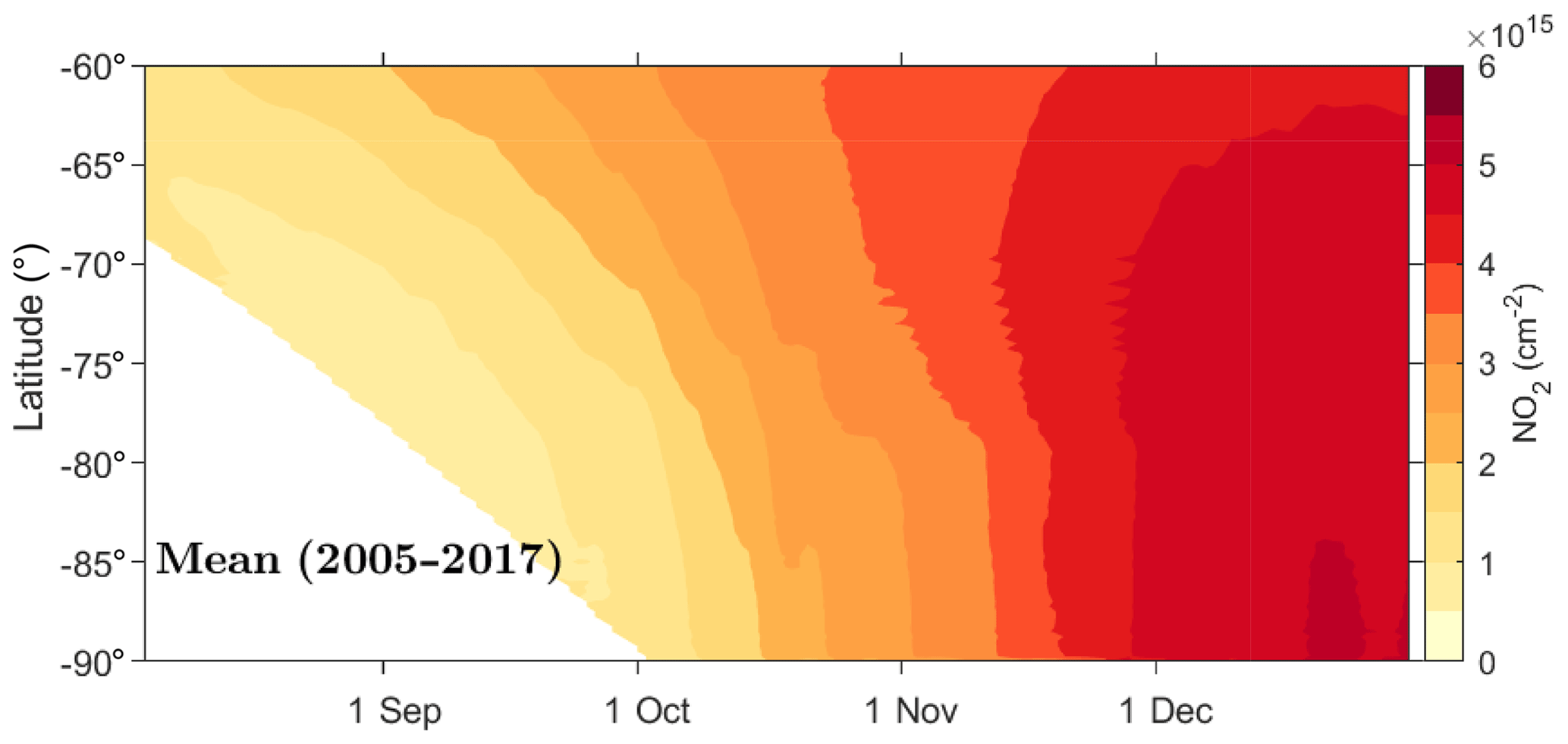
Figure 1 The OMI 3 d running mean zonally averaged NO₂ column for the time period from 2005 to 2017. The contour interval is 0.5×10¹⁵ cm⁻². The white area at high latitudes in August–September indicates polar night conditions, during which OMI observations are not available.

The August–December monthly mean polar (60 to 90^∘ S) average zonal mean NO₂ columns for each year are listed in Table 1.

2.2 MLS observations

We use HNO₃ and temperature profiles from NASA's Microwave Limb Sounder (MLS), which is also onboard the Aura satellite (Manney et al., 2015; Schwartz and Read, 2015). This study uses the version 4.2 product with data screened according to Livesey et al. (2017). The latitude range used here is 60 to around 82^∘ S, and the pressure range used is approximately 100 to 10 hPa. MLS HNO₃ profiles have been validated by Santee et al. (2007), using data from both the HNO₃ 240 GHz radiometer (for pressures ≥22 hPa) and the HNO₃ 190 GHz radiometer (for pressures ≤15 hPa). MLS HNO₃ has a vertical resolution of 3–4 km in the lower–middle stratosphere (used here), and the precision of individual profiles is around 0.6 ppbv in this region. The estimated error in these profiles is no more than 10 %. MLS temperature profiles have been validated by Schwartz et al. (2008) with a precision of around ±0.6 K on individual profiles between 100 and 10 hPa.

2.3 EPP proxy

The geomagnetic activity index, A_p, is a well-established proxy for EPP (see e.g. Matthes et al., 2017; Funke et al., 2014a), and it is used here to estimate the overall levels of EPP for each polar winter under investigation. From 2005 to 2017, the mean of winter A_p was 8.3, reflecting the relatively low overall solar activity during solar cycle 24 (the solar cycle 23 average was 12.9). To estimate the overall EPP activity during each winter, we calculate the mean A_p for the May–August period of each year. These means are referred to as ${\widehat{A}}_{\mathrm{p}}$ hereafter and are provided in Table 1. We designate high ${\widehat{A}}_{\mathrm{p}}$ (H-${\widehat{A}}_{\mathrm{p}}$) winters as those with ${\widehat{A}}_{\mathrm{p}}>\mathrm{8.3}$, i.e. a ${\widehat{A}}_{\mathrm{p}}$ value higher than the average for 2005–2017. Similarly, we designate low ${\widehat{A}}_{\mathrm{p}}$ winters (L-${\widehat{A}}_{\mathrm{p}}$) as those with ${\widehat{A}}_{\mathrm{p}}<\mathrm{8.3}$. The variation in winter ${\widehat{A}}_{\mathrm{p}}$ throughout this study is shown in Fig. 2. This figure captures the 11-year solar cycle fairly well, with a minimum around 2009 and a maximum around 2015.

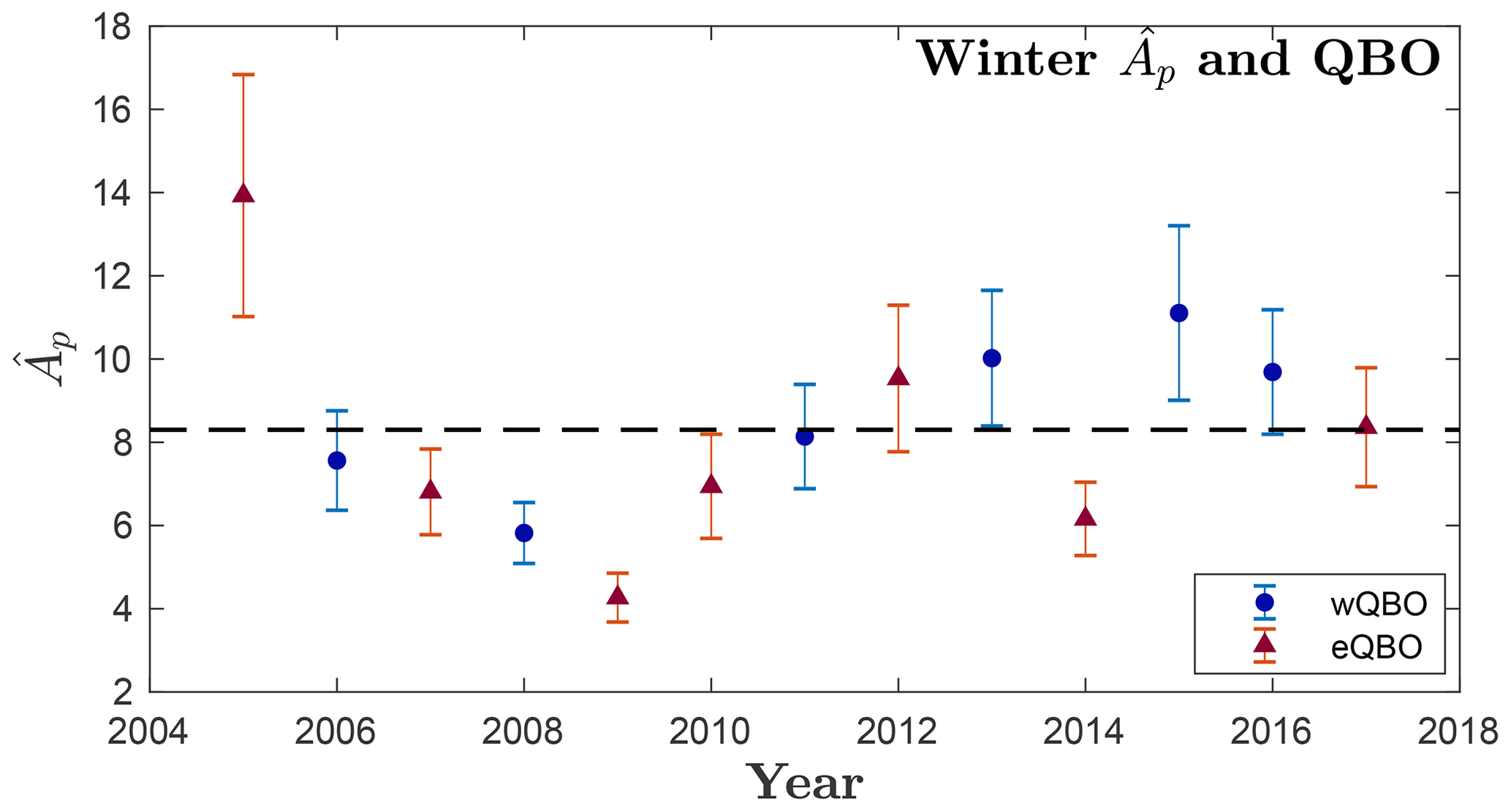
Figure 2 Mean wintertime A_p (${\widehat{A}}_{\mathrm{p}}$) for each year of this study with the error bars indicating 2 times the standard error of the mean (±2SEM). The dashed line indicates the average ${\widehat{A}}_{\mathrm{p}}$ for this study (8.3). The direction of the QBO at 25 hPa in May is indicated: red triangles represent the eQBO, and blue circles represent the wQBO.

Several previous works have used tracer correlations to extract only the NO_x produced by EPP (or NO_y when information on the NO_x reservoirs is available; see e.g. Randall et al., 2007 and Funke et al., 2014b). When tracer information is not available, other works have investigated the variability in odd nitrogen resulting in variability in EPP levels (usually proxied by A_p; see e.g. Seppälä et al., 2007a). Here, we focus on finding evidence of the EPP contribution to column observations. As we do not have mesosphere–stratosphere descent tracer observations available from OMI, we are unable to use the tracer correlation methods. To overcome this, we perform correlation analysis for both latitudinal coverage and polar average NO₂ observations to find evidence of A_p-driven variability in the Antarctic NO₂ column. All correlations between the NO₂ columns and ${\widehat{A}}_{\mathrm{p}}$ are based on the Spearman rank correlation (Spearman ρ), as it more robustly accounts for any non-linear relationships (Wilks, 2011) while still interpreting linear trends where present. Statistical significance is defined here as correlations significant at the ≥95 % level (i.e. p ≤0.05).

2.4 Quasi-biennial oscillation

To investigate the potential QBO effect in the Antarctic atmosphere, we estimate the phase of the QBO from the 25 hPa level zonal mean zonal wind (Naujokat, 1986) near the Equator in May each year. For use of the 25 hPa level in the Southern Hemisphere, see Baldwin and Dunkerton (1998). We designate years when the zonal mean zonal wind direction is easterly as the easterly QBO (eQBO) and westerly as the westerly QBO (wQBO). The QBO direction for each year of the study is indicated in both Table 1 and Fig. 2. Figure 2 illustrates the approximately biennial nature of the oscillation, with the direction changing almost every year.

Table 1 The May–August mean A_p (${\widehat{A}}_{\mathrm{p}}$) ±2SEM, the polar (60 to 90^∘ S) August–December monthly mean cos (latitude)-weighted zonal mean stratospheric NO₂ column density (×10¹⁵ cm⁻²), and the QBO phase (E represents easterly, and W represents westerly) for each year from 2005 to 2017.

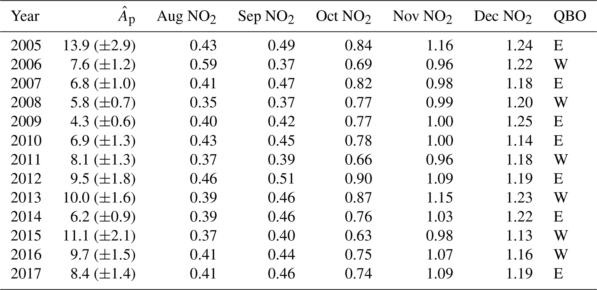
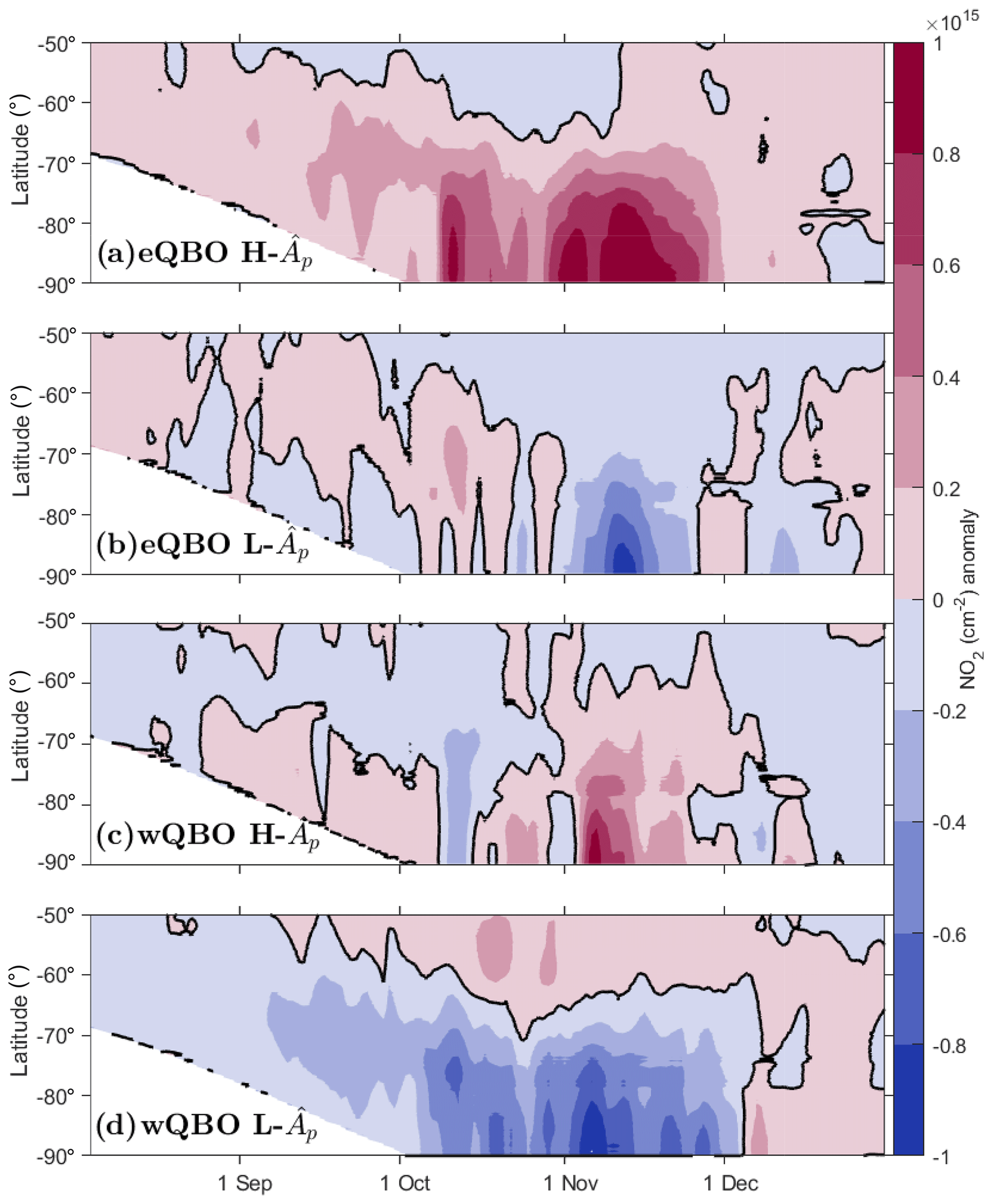
Figure 3 (a) The mean NO₂ anomaly for years with both H-${\widehat{A}}_{\mathrm{p}}$ and eQBO. The contour level is 0.2×10¹⁵ cm⁻² with the black contour representing zero anomaly. Panels (b–d) are the same as (a) but show different combinations of ${\widehat{A}}_{\mathrm{p}}$ and QBO (see figure).

3 Results

3.1 NO₂ anomalies

We first investigate the anomaly from the mean for each of the four different categories of this study: eQBO H-${\widehat{A}}_{\mathrm{p}}$, eQBO L-${\widehat{A}}_{\mathrm{p}}$, wQBO H-${\widehat{A}}_{\mathrm{p}}$, and wQBO L-${\widehat{A}}_{\mathrm{p}}$. This is to show how the NO₂ column evolves in the springtime under the different conditions and to further justify the splitting of years based on the QBO phase. Figure 3 presents the average anomaly, (i.e. the mean, as shown in Fig. 1, is deducted) for each of the four different categories of this study. We can see that the winter ${\widehat{A}}_{\mathrm{p}}$ affects the column NO₂ present in the spring: years with H-${\widehat{A}}_{\mathrm{p}}$ (Fig. 3a, c) have more positive anomalies from August to November, especially at the highest latitudes. In Fig. b and c, the month of October is highly variable, with both panels showing regions of positive and negative anomaly. For low ${\widehat{A}}_{\mathrm{p}}$ years (Fig. 3b, d), early spring is not consistently positive or negative; however, November displays negative anomalies at high latitudes. The combined influence of the QBO and ${\widehat{A}}_{\mathrm{p}}$ appears to be most significant for H-${\widehat{A}}_{\mathrm{p}}$ eQBO years and L-${\widehat{A}}_{\mathrm{p}}$ wQBO years (Fig. 3a, d). These show consistent but opposite behaviour throughout the spring, with H-${\widehat{A}}_{\mathrm{p}}$ eQBO years being the most favourable for NO₂ and wQBO L-${\widehat{A}}_{\mathrm{p}}$ being the least favourable.

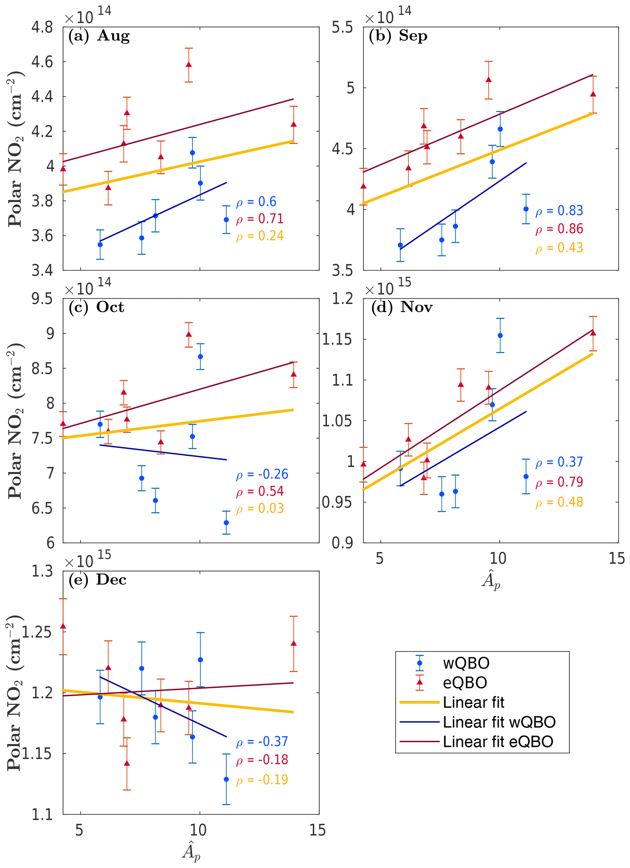
Figure 4 ${\widehat{A}}_{\mathrm{p}}$ vs. the monthly average cos (latitude) area-weighed NO₂ column density averaged over the region from 60 to 90^∘ S (where available, see text) from August to December (months are shown as individual panels). Red triangles indicate years with eQBO, and blue circles indicate years with wQBO. The yellow line shows a least squares linear fit to all data, the red line shows the eQBO years only, and the blue line shows the wQBO years only. The Spearman ρ (correlation coefficient) for each set is shown in each panel using the corresponding colour, e.g. red ρ corresponds to the correlation coefficient for eQBO years. Error bars are ±2SEM.

3.2 Mean SH polar columns

Figure 4 presents the ${\widehat{A}}_{\mathrm{p}}$ and the mean polar (60–90^∘ S) NO₂ column for each year (2005–2017) and for each individual month from August to December. This is to investigate whether a relationship exists between ${\widehat{A}}_{\mathrm{p}}$ size and the NO₂ column, and how this is affected by the QBO phase. The mean polar columns are area weighted by the cosine of latitude. The phase of the QBO in the preceding May is indicated: red triangles correspond to eQBO conditions, and blue circles correspond to wQBO conditions. Least squares linear fits for all years, wQBO years, and eQBO years are included in each panel to guide the eye. The Spearman correlation coefficient (ρ) for each month for all years (yellow) and for eQBO (red) and wQBO (blue) years only are also included in the panels. Note that as the OMI measurement field gradually increases from an initial maximum latitude of around 68^∘ S in August to 90^∘ S by the end of September, the total NO₂ column values do not initially fully encompass the entire polar region (60–90^∘ S). The missing data in August and September are treated as missing values in the mean calculation and, as such, do not contribute to the mean in these figures.

The results shown in Fig. 4 suggests that a correlation between ${\widehat{A}}_{\mathrm{p}}$ and the stratospheric NO₂ column occurs in August, September, and November. This is consistent with Fig. 3. Furthermore, there is a clear positive correlation for eQBO years from August to November, whereas the positive correlation in August and September disappears in October for wQBO years. While the wQBO November linear fit is close to the total fit, the individual years show large variability. In general, wQBO years have consistently lower column NO₂ values, especially in August and September. The generally reduced levels of NO₂ during wQBO conditions is compatible with the analysis of Strahan et al. (2015), which indicated that the altitudes where Funke et al. (2014a) reported EPP-NO_y enhancements in later winter–early spring have consistently lower (higher) levels of the dominant NO_x source, N₂O, during wQBO (eQBO).

To contrast our results with previous extensive work by Funke et al. (2014a), we repeated the analysis presented in Fig. 4 using gigamoles (Gmol, see Funke et al., 2016) for the monthly mean polar NO₂ columns. This figure is included in the Appendix as Fig. A1 and shows the least squares linear fits, with the corresponding parameters given in each panel. This allows us to estimate the EPP contribution to the lower stratosphere (∼15–35 km) NO₂ in the spring, analogous to Funke et al. (2014a). For example, in September (Fig. A1b in the Appendix), the approximate contribution from EPP in eQBO years to the polar stratospheric NO₂ column is +0.023 Gmol/${\widehat{A}}_{\mathrm{p}}$. The largest contribution to OMI lower stratospheric NO₂ from EPP occurs in November, with the corresponding values of +0.073 (eQBO), +0.072 (wQBO), and +0.066 (all years) Gmol/${\widehat{A}}_{\mathrm{p}}$ respectively. Funke et al. (2014a) (see their Fig. 10, showing excess EPP-NO_y in the stratosphere–lower mesosphere in early spring) found an increase in SH polar EPP-NO_y of around +0.0698 Gmol/A_p in September. Contrasting this with our results of +0.066 Gmol/${\widehat{A}}_{\mathrm{p}}$ in November, it seems that a large fraction of the EPP-NO_y detected by Funke et al. (2014a) is maintained in the polar region and is able to reach the lower stratosphere, where it can still be detected as NO₂ in November. Note that Funke et al. (2014a) use a weighted A_p scheme.

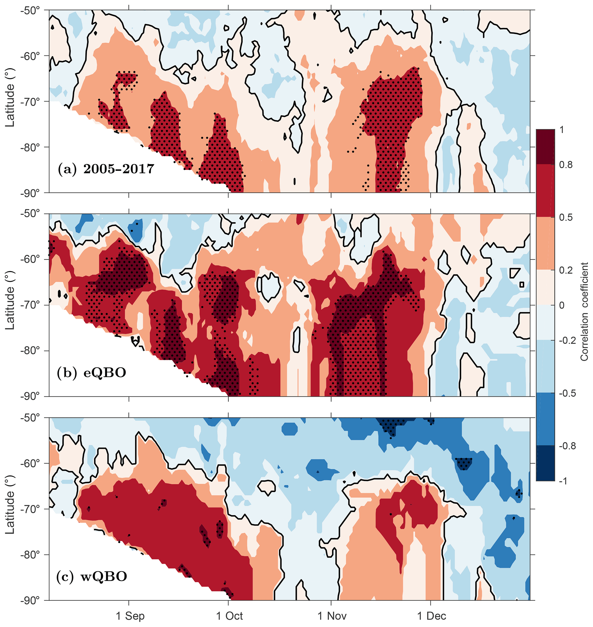
Figure 5 (a) Correlation of ${\widehat{A}}_{\mathrm{p}}$ and the 7 d running mean NO₂ column density for August–December for all years; (b) correlation of ${\widehat{A}}_{\mathrm{p}}$ and the 7 d running mean NO₂ column density for years with eQBO only; (c) correlation of ${\widehat{A}}_{\mathrm{p}}$ and the 7 d running mean NO₂ column density for years with wQBO only. All figures have a 1^∘ latitudinal resolution. Contour levels are shown for [−1, −0.8, −0.5, −0.2, 0, 0.2, 0.5, 0.8, 1], and the zero contour is indicated using black. Stippling shows regions with a correlation significant at the ≥95 % level.

3.3 Latitudinal correlations

Figure 5 shows the latitudinal extent of the correlation between ${\widehat{A}}_{\mathrm{p}}$ and the 7 d running mean NO₂ column for latitudes from 50 to 90^∘ S averaged over 1^∘ latitude bins. Stippling indicates that the correlation is significant at the ≥95 % level. This shows how the correlation between ${\widehat{A}}_{\mathrm{p}}$ and the NO₂ column evolves over time and latitude as well as different QBO phases. Figure 5a presents the correlation when all years are taken into account. A significant positive correlation occurs in late August and varies throughout September; it is then significant again in November. October and December show little to no significant correlation. Figure 5b shows the correlation for eQBO years only. There are areas of statistically significant positive correlations in all months except December. In October, significant correlations only occur at the very beginning of the month. High positive correlations are still present from 60 to 90^∘ S from early to mid-November, providing the first evidence that the indirect EPP-NO_x effect lasts well into the SH spring. Figure 5c presents the correlation for years with wQBO only. While positive correlations are present throughout August and September, only small regions are found to be statistically significant. October marks a shift towards a negative correlation (not statistically significant) at all latitudes. In November, the correlations turn positive once more, but these are once again not statistically significant.

The results shown in Fig. 5 suggest that the NO₂ increases at high polar latitudes in September are due to increased EPP/geomagnetic activity, as strong correlations between NO₂ and ${\widehat{A}}_{\mathrm{p}}$ occur in all panels. They also imply that increases in NO₂ in November can be due to a combination of high EPP activity and eQBO, whereas wQBO appears to reduce the occurrence of any EPP-induced NO₂ increases.

3.4 The polar vortex influence in October

The correlations presented in the previous sections were found to have fewer occurrences of statistical significance in October than the surrounding months. As this time of year marks the typical break-up period of the polar vortex (Hurwitz et al., 2010) and knowing that the descent of EPP-produced NO_x is limited to inside the polar vortex (as previously demonstrated for October by Siskind et al., 2000), we will now investigate October separately, taking the polar vortex into account.

To account for effects from potential asymmetries in the shape of the polar vortex in October in our zonal mean calculations, we repeated the earlier analysis for measurements located inside the vortex. To establish the location of the edge of the polar vortex, we utilized the OMI co-located ozone column measurements (Bhartia, 2012): ozone-depleted air is isolated within the vortex until the vortex break-up, typically in late November (Kuttippurath and Nair, 2017). Based on this, we assume that measurement locations poleward of 50^∘ S with a corresponding stratospheric ozone column of <245 DU are inside the polar vortex. We perform this assessment for every day of October during the study period in order to find the daily vortex extent. This is then used to locate NO₂ that is inside the vortex for every day in October during the study period. An example of how the ozone column and the estimated vortex edge are reflected in the NO₂ column measurement for 1 day of the study (19 October 2014) is shown in Fig. 6. Note that we are unable to use this method on months prior to October due to OMI's viewing method and the ozone column not being low enough to detect a clear vortex edge.

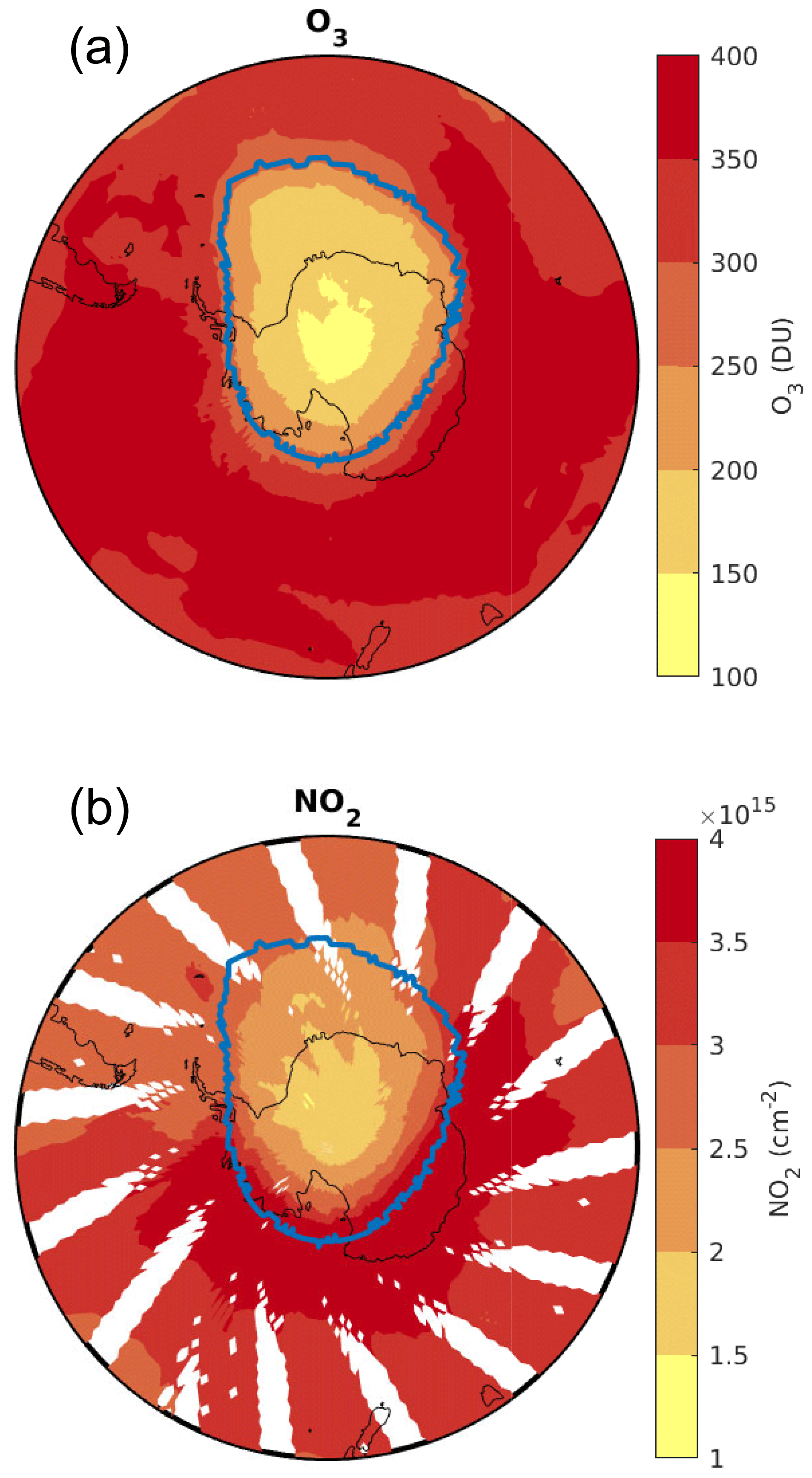
Figure 6 Vortex edge identification based on the OMI ozone column for 19 October 2014. Panel (a) shows the OMI measured ozone column density with the 245 DU contour highlighted. Panel (b) shows the NO₂ stratospheric column with the 245 DU ozone contour highlighted. This method is repeated for each individual day in October throughout the study period.

Figure 7a shows the October results (as in Fig. 4c) when only observations inside the polar vortex are included. For eQBO, we find that the observations are now much closer to the linear fit than in Fig. 4c, implying that the earlier disappearance of correlation was likely due to variations in the shape of the polar vortex in October.

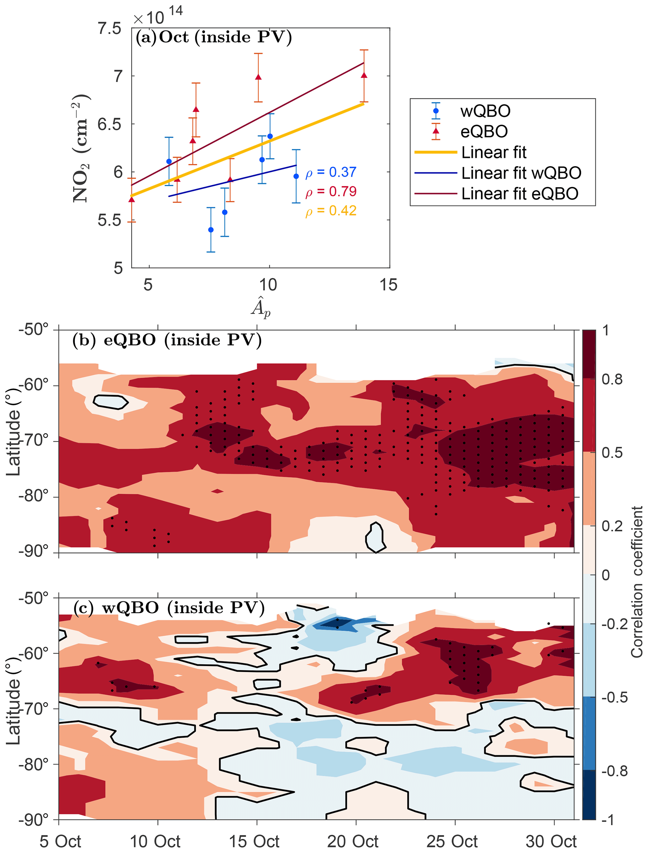
Figure 7 (a) ${\widehat{A}}_{\mathrm{p}}$ vs. the average, cos (latitude) area-weighted NO₂ for the region from 60 to 90^∘ S for observations inside the polar vortex (PV). Red triangles correspond to eQBO years, and blue circles correspond to wQBO years. The yellow line represents a linear fit to all data points, the red line represents a linear fit for eQBO years only, and the blue line represents a linear fit for wQBO years only. ρ values are displayed as in Fig. 4. Error bars indicate the 95 % confidence interval for the mean. (b) Correlation of ${\widehat{A}}_{\mathrm{p}}$ with the 5 d running mean NO₂ column inside the polar vortex for eQBO years. Contour levels are shown for [−1, −0.8, −0.5, −0.2, 0, 0.2, 0.5, 0.8, 1] with an additional black line for the zero contour. The stippling indicates that correlations are significant at the ≥95 % level. Panel (c) is the same as panel (b) but for wQBO years.

Similarly, for the horizontal distribution of the correlations (Fig. 7b), we now find high correlations for eQBO years throughout October. This again implies that the lack of a correlation in October is due to the distorted shape of the polar vortex being smeared out by the calculation of zonal means, and the effect of EPP on the NO₂ column is significant through October. The reappearance of correlations in eQBO years in November in Fig. 5b is likely a mixing effect, with the breakdown of the polar vortex around this time leading to vortex air being mixed with extra-vortex air which results in the NO₂ distribution not being as skewed as it was when contained in the vortex. Figure 7c also shows higher correlation with more instances of significance in wQBO years in October than in Fig. 5c, although this is more variable than in eQBO years (which is consistent with Fig. 5, where wQBO years show lower correlation). Although the A_p index has generally been lower in the past decade than it was during the 1991–1996 period investigated by Siskind et al. (2000), considering observations only in the vortex still shows the same, strong linear relationship found in that study.

4 Discussion

4.1 Influence of the QBO

As shown in Figs. 3, 4, and 5a, our results suggest that the phase of the QBO influences the SH polar EPP-NO_x signal in the spring months. The results of Strahan et al. (2015) suggest that the eQBO phase in early winter leads to increased N₂O between altitudes of ∼24 and 33 km in September: Fig. 1 of Strahan et al. (2015) shows a positive anomaly for N₂O in September in eQBO years (and the opposite for wQBO). Although their designation of the QBO phase differs slightly from ours, this would not largely affect their comparability, as our designations only differ for 1 year of a 10 year study. Our results suggest that although there is an increased pool of N₂O in the polar region during eQBO (contributing to a larger NO₂ column from N₂O oxidation), EPP still contributes a clear fraction to the overall SH polar stratospheric column NO₂ in the springtime. Taking the QBO phase into account, this EPP contribution during spring is generally more pronounced. We note that the high correlation with ${\widehat{A}}_{\mathrm{p}}$ is only present until September for wQBO years, whereas it lasts until November for eQBO years. It is not clear why this is the case for wQBO. A further analysis of possible reasons behind this discrepancy is beyond the scope of this work.

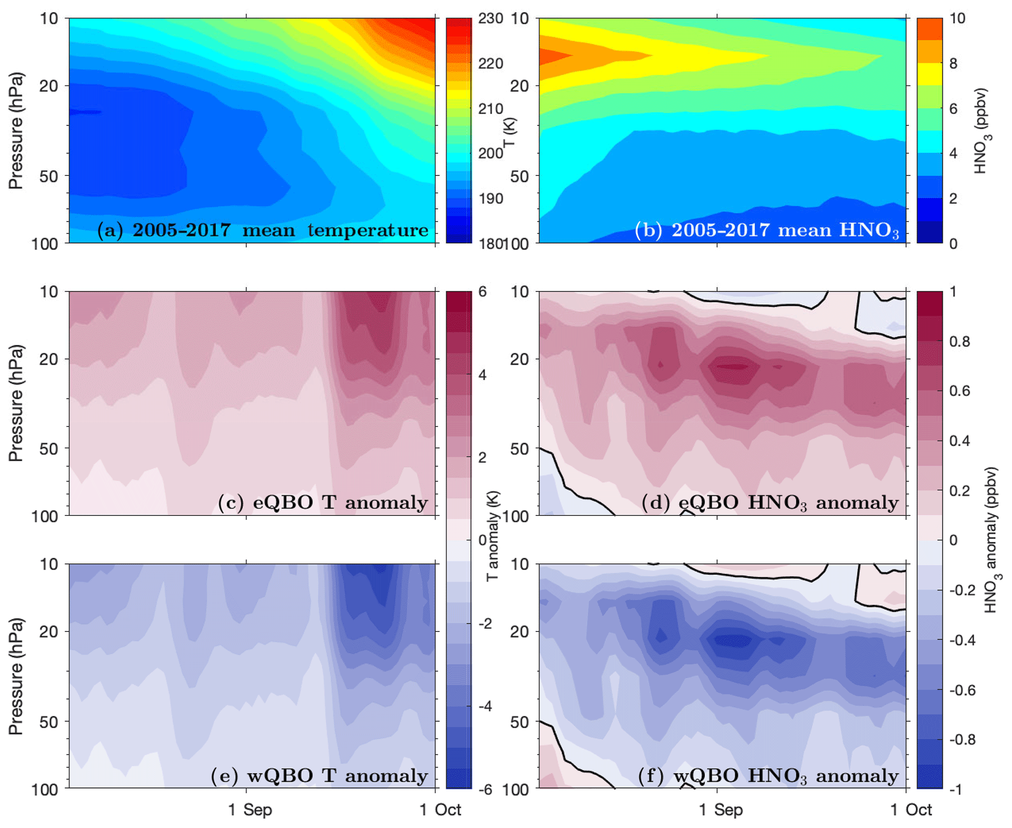
Figure 8 (a) The 3 d running mean MLS temperature from 2005 to 2017 (5 K contour interval), and (b) the 3 d running mean MLS HNO₃ from 2005 to 2017 (1 ppbv contour interval). Panels (a) and (b) are both averaged over the region from 60 to 82^∘ S for the lower stratosphere for the late winter–early spring period from 2005 to 2017. (c) The HNO₃ anomaly (the mean shown in panel a has been subtracted) for years with eQBO (the contour interval is 0.1 ppbv, and the black contour shows the zero anomaly). (d) The temperature anomaly (mean shown in panel b has been subtracted) for years with eQBO (the contour interval is 1 K, and the black contour shows the zero anomaly). Panel (e) is the same as panel (c) but for years with wQBO, and panel (f) is the same as panel (d) but for years with wQBO.

4.2 Possible influence of PSCs and denitrification

Here we discuss possible reasons for the consistently lower amounts of NO₂ in wQBO years found in Fig. 4.

Baldwin and Dunkerton (1998) found that the polar vortex is colder during winters with wQBO. A colder polar vortex results in a higher likelihood of polar stratospheric cloud (PSC) formation (Brasseur and Solomon, 2005). As discussed in Sect. 1, PSCs affect the heterogeneous chemistry in the polar region, leading to the denitrification of the lower stratosphere (Dirksen et al., 2011). One of the possible reasons for the lower NO₂ column during wQBO found here could be enhanced denitrification as a result of lower temperatures in the vortex that bring about enhanced PSC formation. In the following, we will perform a simple analysis to test for signs of this from existing MLS observations, although a more detailed analysis of PSC observations would be required for robust conclusions.

To test whether the QBO phase affects denitrification in the Antarctic stratosphere, we analysed temperature and HNO₃ observations from the MLS (see Sect. 2.2). Figure 8a and b show the mean temperature and HNO₃ respectively, each averaged over the region from 60 to 82^∘ S for 2005–2017 over the late winter–early spring period, i.e. when the polar vortex is coldest and PSCs are forming. Figure 8c and e show the anomalies from the mean temperature for eQBO and wQBO years respectively. Figure 8d and f present the anomaly from the mean HNO₃ mixing ratio for eQBO and wQBO years respectively. The vertical pressure range of all of the panels is 100 to 10 hPa which corresponds to an altitude range of approximately 17 to 32 km. Figure 8 suggests that eQBO years tend to have more HNO₃ (up to 1 ppbv) and a higher temperature (up to 4 K) throughout this period, whereas wQBO years show a consistently negative anomaly in HNO₃ (down to −1 ppbv) and a lower temperature (down to −4 K). Colder temperatures would likely lead to more PSC formation and, thus, more HNO₃ being removed from the stratosphere (more denitrification) in wQBO years (than in eQBO years). It should, however, be noted here that the link between PSC coverage and QBO modulation of polar temperature via the Holton–Tan mechanism is still under debate (see e.g. Strahan et al., 2015).

5 Conclusions

This study provides new evidence of the EPP contribution to the Antarctic stratospheric NO_x column in the late springtime using OMI (Aura) stratospheric NO₂ observations. This is one of the few studies to use stratospheric NO₂ data from OMI and highlights the value of long time series of stratospheric NO₂ from nadir-viewing instruments. Our analysis shows that the influence of the QBO is able to mask the stratospheric EPP-NO_x signal in satellite observations in a way that, to our knowledge, has not previously been accounted for: considering the phase of the QBO makes the contribution from EPP more pronounced in the NO₂ column, and signals of enhanced EPP-NO_x in the polar stratospheric column can be detected until late November.

Previously, Funke et al. (2014a) analysed EPP-NO_y observations, and they were able to attribute SH enhancements with an average A_p dependence of +0.0698 Gmol/A_p to early spring months (September). Here, we show that this reactive nitrogen lingers, entering the lower stratosphere in the form of NO₂ at an average A_p dependence of +0.066 Gmol/${\widehat{A}}_{\mathrm{p}}$ in November.

We present evidence of the contribution from EPP-NO_x in the Antarctic stratosphere at a time when halogen-activated ozone loss is taking place. NO_x is well known to react with both ozone and active halogens, catalytically destroying the former and driving the latter to its reservoirs (Brasseur and Solomon, 2005). Antarctic ozone loss has been found to be reduced in years with eQBO (Garcia and Solomon, 1987) due (at least in part) to the increased vortex temperatures hampering chlorine activation on PSCs (Lait et al., 1989). Our results suggest that as chlorine activation continues to decrease in the Antarctic stratosphere following the Montreal Protocol (Solomon et al., 2016), the total EPP-NO_x (in addition to SPEs as pointed out by Stone et al., 2018) should be accounted for in predictions of Antarctic springtime ozone recovery. Future studies should investigate the role of the larger EPP-NO_x fraction when investigating the net effect of NO₂ on the fragile ozone chemistry in the springtime.

Appendix A

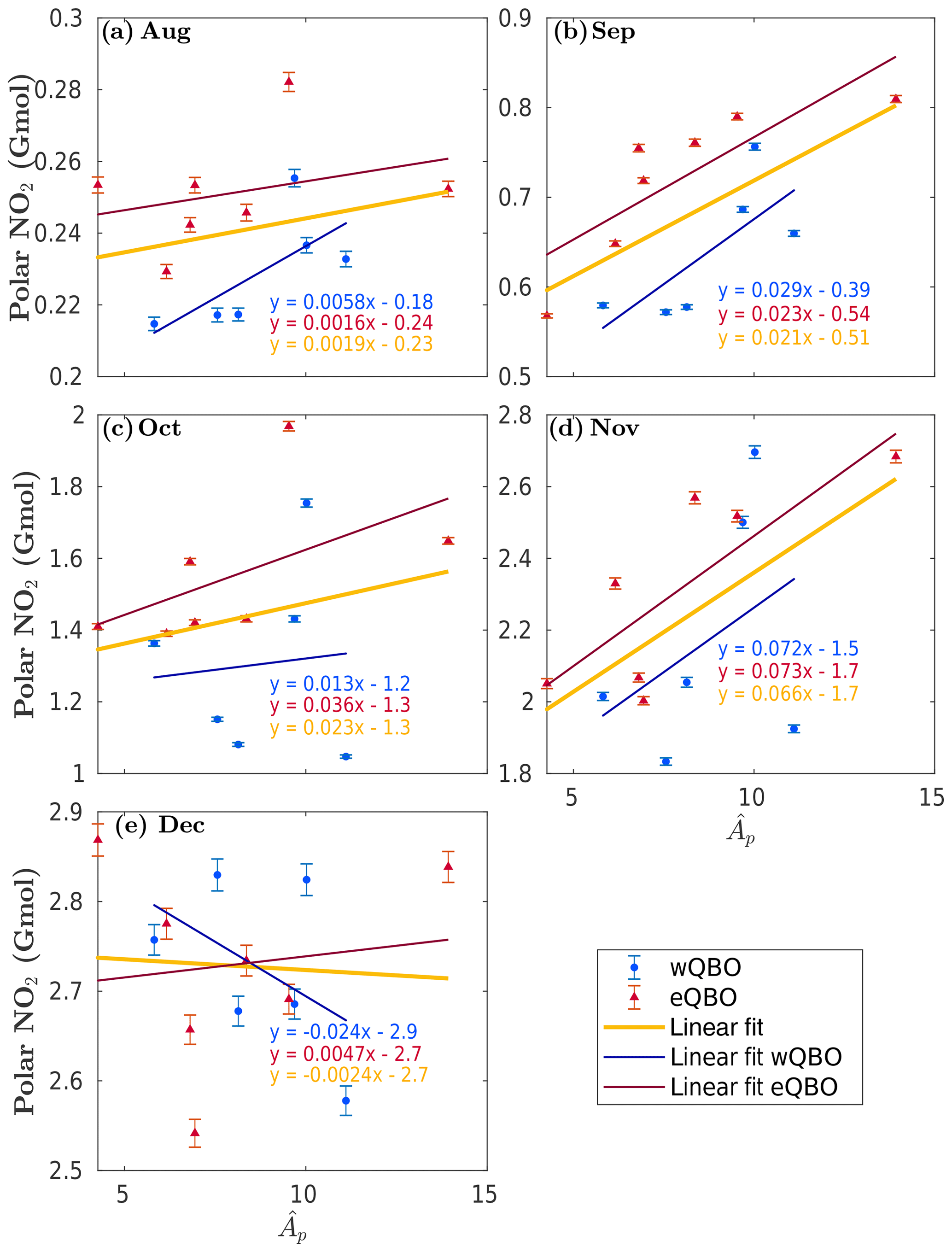
Figure A1 The same as Fig. 4 but with the monthly average polar NO₂ expressed in gigamoles (Gmol). Each panel shows the linear least squares fit to data points (colour coding is the same as that in previous figures), including the fit equations (y= NO₂, $x={\widehat{A}}_{\mathrm{p}}$). Red triangles are years with eQBO, and blue circles are years with wQBO. The yellow linear fit is a best-fit line for all of the data in each plot, the red line fits only eQBO data, and the blue line fits only wQBO data.