the Creative Commons Attribution 4.0 License.
the Creative Commons Attribution 4.0 License.
 | 28 May 2020
Quantifying cloud adjustments and the radiative forcing due to aerosol–cloud interactions in satellite observations of warm marine clouds
Tristan L'Ecuyer
Aerosol–cloud interactions and their resultant forcing remains one of the largest sources of uncertainty in future climate scenarios. The effective radiative forcing due to aerosol–cloud interactions (ERFaci) is a combination of two different effects, namely how aerosols modify cloud brightness (RFaci, intrinsic) and how cloud extent reacts to aerosol (cloud adjustments CA; extrinsic). Using satellite observations of warm clouds from the NASA A-Train constellation from 2007 to 2010 along with MERRA-2 Reanalysis and aerosol from the SPRINTARS model, we evaluate the ERFaci in warm, marine clouds and its components, the RFaciwarm and CAwarm, while accounting for the liquid water path and local environment. We estimate the ERFaciwarm to be Wm−2. The RFaciwarm dominates the ERFaciwarm contributing 80 % ( Wm−2), while the CAwarm enhances this cooling by 20 % ( Wm−2). Both the RFaciwarm and CAwarm vary in magnitude and sign regionally and can lead to opposite, negating effects under certain environmental conditions. Without considering the two terms separately and without constraining cloud–environment interactions, weak regional ERFaciwarm signals may be erroneously attributed to a damped susceptibility to aerosol.
- Article
(1761 KB) - Full-text XML
- BibTeX
- EndNote


Aerosol–cloud interactions (ACIs) and their impact on cloud radiative effects are a vital component of Earth’s radiative balance. Warm clouds, in particular, are susceptible to aerosols, and due to their prevalence and role as “Earth's sunblock”, these interactions are critical for regulating Earth's surface temperature (Platnick and Twomey, 1994). Aerosols entering a cloud may become cloud condensation nuclei (CCN), initiating a domino effect wherein the cloud's droplet number increases, reducing the mean droplet radius, brightening the cloud’s albedo, dampening its ability to precipitate, and, in theory, increasing its lifetime and radiative effect (Twomey, 1977; Albrecht, 1989). However, it remains unknown to what degree aerosols alter warm-cloud radiative forcing as models and observations disagree. Global climate models are prone to uncertainty due to their dependence on parameterizations and inability to explicitly represent all scales of ACIs, while satellite observations have poor temporal resolution, and natural covariances with the environment may influence warm-cloud response to aerosol (Stevens and Feingold, 2009). In order to understand aerosol–cloud interactions and the resulting change in cloud radiative effect, observation-based methods must address the inherent limitations of satellite observations by creating a framework to resolve the interplay between clouds, the environment, and aerosol–cloud interactions (Seinfeld et al., 2016).
Correctly quantifying the effective radiative forcing due to aerosol–cloud interactions (ERFaci) of warm clouds specifically is important to establish a climate sensitivity and identify cloud feedbacks (Bony and Dufresne, 2005; Rosenfeld, 2006; Boucher et al., 2013). It has been understood since the early 1990s that low, warm clouds play a leading role in determining future warming scenarios (Slingo, 1990). The micro- and macrophysical responses of warm clouds to ACIs lead to numerous, poorly understood cloud feedbacks in the Earth system (Gettelman and Sherwood, 2016). Clouds do not exist in isolation (Stephens, 2005). Clouds are part of an interconnected system; changes to one aspect, such as particle size or liquid water content, have a ripple effect on other components of the Earth system. Likewise, clouds can be thought of residing in a “buffered system” where the response of a cloud to aerosol perturbations can be invigorated or diminished depending on the conditions in which it is initiated (Stevens and Feingold, 2009). These interconnections lead to a range of cloud responses to aerosol that depend on the local meteorology and cloud state (Douglas and L'Ecuyer, 2019). Both the short and long timescales of ACIs and their radiative forcing are affected by the interconnections they exist in, meaning constraining the ERFaci of warm clouds must go beyond a single measure of the ERFaci globally and distinguish the individual components of the ERFaci, i.e., the radiative forcing due to aerosol–cloud interactions (RFaci) and cloud adjustments (CA). To account for the challenges in estimating the cloud radiative response to aerosol, we constrain the influences of the local meteorology and cloud state using a method developed in Douglas and L'Ecuyer (2019), hereafter DL19. The ERFaciwarm is separated into the RFaciwarm and cloud adjustments determined with constraints on meteorology following DL19, and estimates of each effect are presented to find the relative contributions of the RFaciwarm and cloud adjustments to the ERFaciwarm. The present study expands upon work done in DL19 by specifying what aspects of the cloud lead to changes in the cloud radiative effect (CRE), whether that be the brightness or cloud extent or both, and whether these changes can negate each other, such as when a cloud shrinks but the brightness increases.
Warm clouds, like marine stratocumulus and trade cumulus, are the prevailing cloud type over the oceans and dominate aerosol–cloud interactions (Gryspeerdt and Stier, 2012). Marine stratocumulus over the cold upwelling waters, such as off the west coast of Africa, persist for long periods of time in the stable, low marine boundary layers (Wood, 2012). Cumulus form from marine stratocumulus to cumulus transitions and in the equatorial region as trade cumuli (Sandu and Stevens, 2011). The sheer abundance and bright albedo of warm clouds make them important to the radiative balance of Earth, and it should be no surprise that warm clouds contribute the largest amount of forcing to the ERFaci (Christensen et al., 2016). Marine stratocumulus have been the primary focus of aerosol–cloud–radiation interactions due to their sheet-like, “homogeneous” structure, pervasiveness (∼25 % of the Earth at any moment), location near anthropogenic continental emissions, and susceptibility to changes in their CCN (Hahn and Warren, 2007; Platnick and Twomey, 1994).
The warm-cloud albedo has the largest response to aerosol compared to mixed-phase or ice-phase clouds (Christensen et al., 2016). Twomey was the first to hypothesize the high susceptibility of entirely liquid clouds to aerosol using a simple cloud model; work since then has confirmed this as the basis of RFaci (Twomey, 1977). Observation- and model-based studies focus on the albedo effect because it is a macrophysical manifestation of microphysical processes. An increase in CCN and decrease in mean droplet radius greatly increase the cloud albedo and, as such, have significant implications for the radiative balance. The radiative forcing of the albedo effect, or the sudden microphysical response to aerosol loading (RFaci), is dependent on the activation and eventual microphysical initiation of aerosol as cloud droplets, which can be influenced by local dynamics, the stability of the boundary layer, and the initial cloud state (Su et al., 2010). “Model” conditions simulated by Twomey only exist in the most pristine, stable southern oceans (Gryspeerdt et al., 2017; Hamilton et al., 2014). Depending on the region studied, aerosol can increase the cloud albedo as expected or in certain cases, lead to a dimming effect, such as when aerosol loading reaches a critical point or the local meteorology regulates the sign and/or magnitude of ACIs (Gryspeerdt et al., 2019; Christensen et al., 2014). Studies conflict to what degree the RFaci dominates the ERFaci, in part because the cloud acts as a buffered system and mitigates the RFaci depending on the thermodynamic conditions, making the quantification of the RFaci particularly challenging (Goren and Rosenfeld, 2014; Feingold et al., 2016; Stevens and Feingold, 2009).
Efforts to understand the other component of the ERFaci, cloud adjustments, have been similarly clouded in uncertainty. Cloud lifetime and extent are highly susceptible to aerosol (Dagan et al., 2018). Models have shown that aerosol affects the distribution of liquid throughout the cloud and vertical motion within the cloud, greatly perturbing the cloud’s lifetime, precipitation, and extent (Ramanathan et al., 2001; Dagan et al., 2016). Aerosol can act to increase the lifetime of clouds through delayed collision coalescence or decrease the lifetime through evaporation–entrainment and induced cloud feedbacks (Albrecht, 1989; Small et al., 2009). A satellite observation-based study of ship tracks showed clouds experience a expansion or shrinking of cloud extent depending on whether the clouds are at an open or closed state and the background state of the aerosol (Chen et al., 2015). The cloud adjustment response depends on the cloud state and a sequence of reactions dictated by the environment (Gryspeerdt et al., 2019). As such, cloud adjustments remain the largest source of variability in ERFaci in global climate models (Fiedler et al., 2019).
To account for influences and variation in the ERFaciwarm, RFaciwarm, and warm-cloud adjustments, we constrain the liquid water path, relative humidity of the free atmosphere, and stability of the boundary layer and covariances between them before evaluating the susceptibility of the effect in the same fashion as DL19. These constraints are held fixed first on a global and then on a regional basis to diagnose regime-specific then regionally specific responses. Finally, the decomposed ERFaciwarm, or the sum of the RFaciwarm and warm-cloud adjustments, is calculated, with constraints on the environment and cloud state, for precipitating and non-precipitating scenes on a regional basis. Our methodology aims to reduce biases by accounting for the regionally specific aerosol and thermodynamic conditions (Feingold, 2003). The relationship between aerosol and cloud response has been proven to be sensitive to regional features like aerosol type or meteorology (Twohy et al., 2005; Chen et al., 2014) (DL19). Aerosol–cloud interactions experience a nonlinear relationship with liquid water path; therefore it is important to separate this complex relationship from ACIs and the associated forcing in order to reduce the effects of this nonlinear relationship on our results (Gryspeerdt et al., 2019).
2.1 Data
Collocated satellite observations of cloud shortwave effect, cloud fraction, and aerosol index are obtained by NASA A-Train satellites Aqua, CloudSat, and the Cloud-Aerosol Lidar and Infrared Pathfinder Satellite Observation (CALIPSO) from 2007 to 2010. The NASA A-Train was intentionally created to maximize the synergy between different satellite products in order to improve our understanding of clouds, aerosols, and the environment (L'Ecuyer and Jiang, 2011). Observations of marine warm clouds and aerosols from the Cloud Profiling Radar (CPR) and Moderate Resolution Imaging Spectroradiometer (MODIS) aboard CloudSat and Aqua, respectively, are utilized to evaluate the effects of aerosol–cloud interactions on the radiative properties of clouds including their albedo and extent.
CloudSat was launched to an orbit collocated with Aqua and other A-Train satellites in 2006. The CPR on CloudSat is a 94 GHz radar with a ∼1.7 km along-track, 1.4 km cross-track resolution, and 480 m vertical resolution (Stephens et al., 2018; Tanelli et al., 2008). A number of cloud properties can be inferred using the CPR backscatter including cloud top height, cloud type, and accompanying radiative effects.
An along-track warm-cloud fraction is defined using cloud top height from 2B-CLDCLASS-LIDAR and freezing level from 2C-PRECIP-COLUMN. 2B-CLDCLASS-LIDAR combines CloudSat's CPR with CALIPSO lidar observations in order to discern even the thinnest clouds. At each pixel, the cloud fraction is defined by the amount of cloud uptrack and downtrack of that pixel at a 12 km scale, chosen to approximate the scale of marine boundary layer processes and accentuate small-scale changes in extent compared to other large sizes (e.g., ). Using a smaller scale such as 12 km for cloud fraction will allow even minute changes in the cloud extent to be detected by our methodology; using a larger size such as 96 km (∼1∘) may diminish cloud breakup processes within large stratocumulus decks or minimize effects on trade cumuli. 2B-CLDCLASS-LIDAR includes collocated Cloud-Aerosol Lidar with Orthogonal Polarization (CALIPSO) satellite lidar backscatter measurements to identify thin, shallow clouds that may escape detection by the CPR (Sassen et al., 2008). Cloud top heights from 2B-CLDCLASS-LIDAR, defined using a combination of collocated lidar and CPR measurements, are required to be below the freezing level (Haynes et al., 2009). The freezing level of 2C-PRECIP-COLUMN is obtained from European Centre for Medium-Range Weather Forecasts (ECMWF) analyses and is used to separate warm from mixed- and ice-phase clouds. Focusing only on warm-phase clouds helps reduce the uncertainty associated with retrievals of mixed- and ice-phase clouds.
Cloud fraction is combined with shortwave top of atmosphere forcings from the CloudSat 2B-FLXHR-LIDAR product to approximate the effect of aerosol on albedo. 2B-FLXHR-LIDAR uses a combination of CPR and CALIPSO measurements along with MODIS cloud properties and atmospheric conditions from ECMWF as input to a radiative transfer model that computes top of atmosphere shortwave fluxes that have been shown to agree well with CERES observations (Henderson et al., 2013). The mean shortwave flux at the top of atmosphere is weighed by a mean incoming solar radiation at the top of atmosphere in our analysis to account for diurnal variation in incoming solar radiation not sampled by the sun-synchronous A-Train orbit.
We use aerosol index (AI) as a proxy for aerosol concentration from MODIS. The AI is the product of the Angstrom exponent, calculated using aerosol optical depth (AOD) at 550 and 870 nm and the AOD at 550 nm. AI has been shown to have a higher correlation with CCN compared to AOD (Stier, 2016; Hasekamp et al., 2019). Cloudy scene AI is determined by interpolating between clear scenes along track. This interpolation may reduce the accuracy in completely overcast scenes; however for most scenes where cloud fraction is <1, this interpolation should be sufficiently accurate. Aerosol swelling in high humidity environments also leads to some uncertainty in AI but should be limited to select high-humidity environmental regimes. Preindustrial aerosol information is provided by Spectral Radiation-Transport Model for Aerosol Species (SPRINTARS), an atmosphere–ocean general circulation model (Takemura et al., 2000). Preindustrial aerosol errors lead to the majority of uncertainty in ACIs due to uncertainties in transport, source, and concentration of preindustrial aerosol conditions (Chen and Penner, 2005).
The sign and regional variations in susceptibilities found using MODIS AI shown within this study were evaluated against susceptibilities found using MACC and SPRINTARS aerosol in order to qualitatively scrutinize any error due to aerosol retrieval (Douglas, 2017). MACC and SPRINTARS provide independent aerosol estimates not susceptible to swelling, instrument sensitivity, or retrieval error.. The fact that our results were qualitatively similar using modeled aerosol provides confidence that the derived susceptibilities shown are not simply an artifact of using satellite-derived AI.
The analysis is constrained to clouds with liquid water paths (LWPs) between 0.02 to 0.4 kgm−2 using the Advanced Microwave Scanning Radiometer for Earth Observing Satellite (AMSR-E), an instrument aboard Aqua that infers water vapor and precipitation amounts using six microwave frequencies over a ∼14 km2 area (comparable to the averaging scale of our cloud fraction) (Parkinson, 2003; Wentz and Meissner, 2007). While the footprints of CloudSat and AMSR-E do not perfectly overlap, the AMSR-E LWP is used to establish a scene-based constraint on the clouds in order to better consolidate our observations into regimes. AMSR-E's footprint is within ∼2.5 km of CloudSat's track, meaning both sensors are observing the same liquid clouds (Lebsock and Su, 2014). Imposing these LWP limits in place removes only ∼1 % of observations leaving over 1.8 million satellite observations for analyses but avoids possible skewing by extremely thick, bright clouds or extremely thin, dim clouds.
Environmental information to define local meteorological regimes is provided by the Modern-Era Retrospective analysis for Research and Applications, version 2 (MERRA-2) reanalysis (Gelaro et al., 2017). To broadly characterize large-scale environmental conditions, MERRA-2 temperature and humidity profiles are collocated by taking the environmental profile within 30 min of a CloudSat overpass and within ∘ latitude and longitude. Vertical profiles of humidity and temperature are used to calculate the estimated inversion strength (EIS) of the boundary layer and the relative humidity at 700 mbar (RH700) to represent the humidity of the free atmosphere (Wood and Bretherton, 2006). By simultaneously stratifying the observations by LWP, RH, and EIS, the analysis directly accounts for covariability between LWP and the local environment by separately evaluating the susceptibility of each environmental regime within distinct LWP limits (Douglas and L'Ecuyer, 2019).
Clouds are separated into precipitating and non-precipitating regimes using CloudSat's 2C-PRECIP-COLUMN precipitation flag. Clouds with a 0 precipitation flag, no precipitation detected, are designated as non-precipitating. Precipitating clouds are separated using flag 3, where rain is certain (Haynes et al., 2009). Our precipitating clouds include a majority of the drizzling cases, as CloudSat's 2C-PRECIP-COLUMN's threshold for drizzle is −15 dB, which should capture all but the lightest drizzling clouds (Stephens and Wood, 2007).
2.2 Methodology
In DL19, environmental and cloud state regimes were imposed on a regional basis in order to identify regime-specific behavior of aerosol–cloud–radiation interactions. Within each regime, we regressed the cloud radiative effect (CRE) against AI in order to find the susceptibility of warm-cloud radiative properties to aerosol. We use these same susceptibilities within Sect. 3.1 to quantify the total warm, marine ERFaci. DL19 found that the susceptibility varies regionally and by regime; however the ERFaciwarm depends on the magnitude to which aerosol has increased since preindustrial times. Further, the ERFaciwarm does not diagnose what characteristics of the cloud are causing the effect, prompting us within this paper to decompose the ERFaciwarm into the effects on the albedo and the effects on cloud extent.
The mean shortwave flux at the top of the atmosphere from CloudSat’s 2B-FLXHR-LIDAR along with our definition of warm-cloud fraction from 60∘ S to 60∘ N are used to define the RFaciwarm and cloud adjustment terms of the ERFaciwarm. We first calculate the ERFaciwarm on a regional basis with regime constraints using estimates of the susceptibility of the warm CRE to aerosol from DL19 and preindustrial and present-day AI from SPRINTARS. We then use a partial derivative decomposition to separate out the RFaciwarm and cloud adjustment terms. These terms are evaluated globally as susceptibilities with constraints on the local meteorology and cloud state following the methodology of DL19. The RFaciwarm and cloud adjustments are evaluated regionally with constraints on cloud state and local meteorology. The decomposed ERFaciwarm is evaluated for precipitating and non-precipitating scenes to account for the potential effects of precipitation on ACIs. Finally, the sum of the RFaciwarm and cloud adjustments, i.e., the decomposed ERFaciwarm, is compared against the first estimate of the ERFaciwarm.
2.3 Regimes
Following DL19, the ERFaciwarm and components are evaluated within a constrained space on both a global and regional scale. LWP is held approximately constant using a set of 12 LWP limits on a global basis and five LWP limits on a regional basis. This is in line with the original work of Twomey (1977), which surmised that only for a fixed LWP will the cloud albedo increase in more polluted conditions. The local meteorology is defined by the stability of the boundary layer and the relative humidity of the free atmosphere. Both the stability, characterized by the estimated inversion strength, and the relative humidity of the free atmosphere, defined at the 700 mbar level, have been shown to influence the sign and magnitude of the susceptibility of the CRE to aerosol (Wood and Bretherton, 2006; Ackerman et al., 2004; De Roode et al., 2014). The resulting regimes isolate the susceptibility of the cloud to aerosol under controlled conditions. Buffering can entail the cloud being too thick and impervious to changes due to aerosol due to its high LWP, offsetting and opposite reactions of the cloud resulting in reduced mean signal, or the environment acting to dampen the cloud reaction, such as an unstable boundary layer reducing the impact of aerosol on cloud lifetime (Fan et al., 2016; Stevens, 2007). Using EIS and RH700 does not guarantee to limit all covariability between the environment, aerosols, clouds, and their interactions. Some covariability may still exist, such as surface winds that may affect both clouds and aerosol (Nishant and Sherwood, 2017). These constraints only account for the major environmental controls on clouds and aerosol–cloud interactions; some more minor or less common environmental controls may still exert an influence on our results.
While binning our observations by environmental regime should control for some modulation the environment has on aerosol–cloud interactions, it does not fully capture aerosol–environment interactions. For example, in some regions such as off the coast of Africa, biomass burning results in smoke layers that absorb incoming radiation and warm the atmosphere (Cochrane et al., 2019). This could affect the humidity and temperature of the local environment. Environmental regime constraints would capture how the altered environment may regulate aerosol–cloud interactions, but separation into such regimes does not address how the aerosol has impacted the environment.
2.4 Decomposing the ERFaci
A Newtonian-based method is employed to represent the ERFaciwarm as a sum of its parts, i.e., the RFaciwarm and cloud adjustments. A positive ERFaciwarm, RFaciwarm, or cloud adjustment denotes a damped cooling effect of the cloud, while a negative sign denotes an additional cooling due to aerosol–cloud interactions. If the shortwave cloud radiative effect is the product of the cloud fraction (CF) and the cloudy sky shortwave flux at the top of the atmosphere (SWCloudy),
then, taking the derivative of the CRE with respect to the log of aerosol index, we find the effective radiative forcing due to aerosol–cloud interactions (ERFaciwarm) or the change in the CRE with respect to aerosol.
where Δln(AI) is the change in ln(AI) from preindustrial to present-day conditions derived from SPRINTARS. SPRINTARS is a 3D aerosol model that includes emission, advection, diffusion, chemistry, wet deposition, and gravitational settling of multiple species of aerosol driven by a general circulation model developed by the University of Tokyo (Takemura et al., 2000, 2005). The results shown herein depend on the emissions scheme from SPRINTARS; if the model were altered, it is possible that the total forcing would change due to different Δln(AI).
All susceptibilities are found using MODIS AI, while only the Δln(AI) term uses SPRINTARS modeled aerosol. The lowest 12 % of aerosol indices are ignored when determining a susceptibility, as these have been shown to have little to no correlation with CCN compared to higher indices (Hasekamp et al., 2019). Error in MODIS AI estimates adds the greatest source of uncertainty in the observationally based portion of this study; however, signals derived are all robust enough to be observed even when random error is added to 10 % of the AI estimates. The regressions within all regime constraints, from only meteorological to regional, remain robust for all susceptibilities when 10 % of the AI estimates were randomly assigned. The same relationships can be qualitatively observed when SPRINTARS AOD is used in lieu of MODIS AI (Douglas, 2017). The susceptibility can be obtained directly from satellite estimates of top-of-atmosphere clear-sky and all-sky fluxes and aerosol index or further decomposed into separate albedo and cloud fraction responses using Eq. (1). Applying the chain rule to Eq. (2), combined with the definition of CRE from Eq. (1), gives
where the overbars represent means. The sum of the righthand terms represent the decomposition susceptibility:
The first term of Eq. (4) represents the cloud adjustment susceptibility to aerosol, which to first order is the effect of aerosol on the cloud extent:
The cloud adjustment forcing is the product of the cloud adjustment susceptibility λCA and the change in AI from preindustrial to current times Δln(AI):
The cloud adjustment susceptibility (λCA) is described by its most notable effect, the enhancement and sustainment of clouds as a result of precipitation suppression. We define the cloud adjustments as the product of the change in cloud fraction with respect to aerosol index and the mean cloud shortwave forcing. By multiplying by the mean cloud shortwave forcing, a change in cloud extent is converted to a change in the reflected shortwave. While this term does not explicitly account for precipitation, we separate clouds by rain state and determine the difference in the RFaciwarm and cloud adjustments between precipitating/non-precipitating clouds; this difference is likely close to the overall effect of precipitation on aerosol–cloud-radiation interactions.
This cloud adjustment term accounts for the main process, the change in extent of clouds by aerosol; however many other studies define the cloud adjustment term by the change in LWP by aerosol. We choose to instead focus on the expansion or shrinking of clouds by aerosol and constrain any LWP effects. Research has yet to establish how and where LWP increases or decreases due to aerosol–cloud interactions; focusing on the changes to cloud extent reduces the error in the adjustment term due to this uncertainty. The second term on the righthand side of Eq. (4) represents susceptibility of warm-cloud radiative forcing due to aerosol–cloud interactions (RFaci):
where the associated forcing is the product of the RFaciwarm susceptibility λRFaci and the change in AI from preindustrial to current times Δln(AI):
The RFaciwarm susceptibility is the change in the shortwave effect owing to changes in cloud droplet radius, an immediate, fast response. The outgoing shortwave radiation for cloudy scenes depends on the cloud albedo; a brighter, whiter cloud will reflect more incoming solar radiation, increasing SWCloudy at the top of the atmosphere. SWCloudy is weighted by the annual solar insolation cycle in order to normalize the term and reduce the impact of changes in the incoming solar flux. RFaciwarm is weighted by mean cloud fraction since the net effect of brighter clouds depends on how extensive they are. Finally, to account for the dependence of each susceptibility (RFaci, CA, and total) on the meteorology and cloud state, each susceptibility (λs from above) is evaluated in distinct EIS, RH, and LWP regimes regionally. The product of each susceptibility and Δln(AI) is the resulting forcing of the aerosol–cloud–radiation interaction:
where is the weighting factor, N is the number of limits imposed, and λ is the susceptibility being evaluated (ERFaciwarm, RFaciwarm, or CA) regionally (NReg) with constraints on LWP, EIS, and RH700. weights the ERFaciwarm, RFaciwarm, and cloud adjustments by the number of observations in each regime and also by the areal size of the region.
Constraints on LWP reduce the secondary effects of aerosol on LWP or LWP on susceptibility, as aerosol can result in thicker clouds, and thicker clouds may have a damped reaction to aerosol. Constraining the meteorology separates signals forced by aerosol and the environment (Stevens and Feingold, 2009). On a global scale the approach outlined in DL19 identifies regime-specific behavior; when applied on regional scales, the regimes allow a process level understanding of the mean regional behavior (Mülmenstädt and Feingold, 2018). This approach is optimal for our satellite-based observations where larger-scale parameters like AOD, AI, and cloud extent are less impacted by retrieval errors than specific properties of the aerosol.
The RFaciwarm and cloud adjustment susceptibilities are first understood with limits on the environment and cloud states on a global scale. Their individual forcings, or the product of the susceptibility and Δln(AI), are then found with constraints on the environment and cloud state regionally and contrasted against initial estimates of the ERFaciwarm evaluated under the same constraints. The susceptibility estimates are not forcings. Forcings are the product of the susceptibilities (λRFaci or λCA) and the change in the aerosol index from preindustrial times to current estimates, Δln(AI)). It is possible that even these estimates of forcing are slightly different than the definition of forcing from the IPCC or model-based studies which differentiate between top-of-atmosphere forcings in polluted vs. non-polluted GCM runs (Penner et al., 2011). The sum of these forcings, which we will term the decomposed ERFaciwarm, is contrasted with the simple expression for ERFaciwarm evaluated directly using Eq. (2). By separating out the individual components of the ERFaciwarm, the physical processes of aerosol–cloud–radiation interactions can be better understood. The difference between the ERFaciwarm and the decomposed ERFaciwarm represents uncertainty in the linear decomposition owing to covariability, nonlinearity, and other effects not quantified by our approach. In reality, there should be a covariability term at the end of Eq. (4) to relate how a change in RFaciwarm may affect cloud adjustment processes or vice versa; however a limitation of satellite observations is that they cannot temporally relate events, meaning covariance between the two terms cannot be accurately quantified (Seinfeld et al., 2016). We focus on the main cloud adjustment, the effect of aerosol on the cloud extent/lifetime; however other cloud adjustment effects exist that our simple calculation of a decomposed ERFaciwarm misses, such as how precipitation suppression directly leads to changes in cloud extent or how suppression could lead to a later invigorated state of the cloud and faster dissipation.
Precipitation is indicated by the 2C-RAIN-PROFILE rain rate along the entire 12 km track segment (L'Ecuyer and Stephens, 2002). The decomposition susceptibility is found for precipitating and non-precipitating scenes globally using Eq. (9). Only the decomposition terms are found separately for precipitating and non-precipitating pixels. The CERES footprint is larger than the CloudSat's, meaning that while CloudSat could see an entire 12 km along-track segment with no rain, the CERES footprint could still contain rain and influence the regression.
Uncertainty in each effect is found first by assuming the uncertainty in the observations lies in the AI, then by assuming a majority of the overall uncertainty in the ERFaciwarm from error in the preindustrial aerosol concentration estimates (Hamilton et al., 2014). Error is added randomly to AI to find how aerosol swelling or inaccurate retrievals of aerosol near cloud could alter susceptibility estimates. Aerosols swell in the vicinity of clouds, which increases their size and affects the MODIS-retrieved AI (Christensen et al., 2017). To assess how significantly this may affect results we have randomly added errors of 10 % to our AI estimates and re-derived all signals with all regime constraints. Even with error in AI, the signals within our environmental and LWP regimes are robust. Uncertainty in the observations is most likely to come from the AI as CloudSat 2B-FLXHR-LIDAR fluxes have been shown to have at most ∼10 Wm−2 error in shortwave top-of-atmosphere fluxes (Henderson et al., 2013). The error from AI is then combined with randomly adding error to the preindustrial AI estimates from SPRINTARS to quantify how error in the preindustrial aerosol may lead to uncertainty in the ERFaciwarm, RFaciwarm, and cloud adjustments. Overall, the majority of uncertainty in any ERFaci estimate lies in the preindustrial aerosol estimate (Chen and Penner, 2005; Carslaw et al., 2013; Stevens, 2013).
3.1 Estimate of the ERFaci
The warm-cloud ERFaci, or the effective radiative forcing due to aerosol–cloud interactions, is −0.32 Wm−2 when found with constraints on the liquid water path, stability, and free atmospheric relative humidity applied regionally. As stated before, a negative ERFaci/RFaci/cloud adjustment denotes additional cooling due to aerosol–cloud interactions. Figure 1 shows each component of Eq. (9) and the resulting regional distribution of the ERFaciwarm. The ERFaciwarm is found by applying Eq. (2) regionally with regime constraints following DL19. This is within the range reported by the fifth IPCC report (−0.05 to −0.95 Wm−2) but suggests the net cooling effect is toward the lower end of the expected range. Note, however, that this estimate neglects contributions from cold- or mixed-phased clouds and land regions (Boucher et al., 2013). This first estimate of the ERFaciwarm represents the sum of all effects of aerosol on the warm-cloud radiative effect with no distinction between the RFaciwarm and CAwarm and is representative of how aerosol–cloud interactions may be altering the current radiative budget (Carslaw et al., 2013).

Figure 1(a) The change in aerosol index from SPRINTARS from the preindustrial to present day, (b) adapted from DL19, and (c) the associated ERFaciwarm found using Eq. (2) found with constraints on LWP, EIS, and RH700 ( Wm−2) using susceptibilities from DL19 (b) without areal weighting.
As expected, marine stratocumulus decks in the southeast Pacific and South Atlantic exhibit the largest ERFaciwarm, exceeding −3.0 Wm−2 off the coast of Chile. The peak cooling is observed in the Southern Hemisphere, where the marine stratocumulus cloud decks subsist due to the strong inversions and cool sea surfaces (Wood, 2012). The storm track regions in the North Atlantic exhibit a slight cooling, as do the marine stratocumulus off the coast of California; however the Southern Hemisphere dominates the cooling effect. Some regions where dimming occurs are amplified by the change in emissions of the region, such as the Asian coast.
Interestingly, ACI is responsible for a net warming of as much as 0.6 Wm−2 in the tropical Atlantic and Indian oceans. Diagnosing the cause of this warming cannot be done through the ERFaciwarm, as it is impossible to accurately attribute it to a reduced albedo or cloud adjustment process. This signature, in particular, motivates decomposing the ERFaciwarm into the RFaciwarm and cloud adjustment components to allow the instantaneous albedo response to be separated from slower cloud processes. The physical processes resulting in a warming differ between the two components as the cloud adjustments are on a macrophysical scale, while the RFaciwarm is due to microphysical interactions between aerosol and CCN. The decomposition in Eq. (3) allows the specific underlying physical processes responsible for this positive (warming) forcing to be assessed regionally.
The change in aerosol index is most notable off the coast of Asia and along the European coasts. Emissions from large coastal cities lead to large increases in AI, particularly changes in sulfuric aerosol (McCoy et al., 2017). The AI may have decreased off the coast of Australia due to the overall aerosol size increasing, which would decrease the Angstrom exponent and therefore AI (Carslaw et al., 2017). The Northern Hemisphere has had much larger changes in AI since preindustrial times compared to the Southern Hemisphere due to the differences in anthropogenic activity between the two hemispheres. While the Southern Hemisphere has not experienced the same extreme changes in AI as the coast of Asia, the strong susceptibility of these warm clouds to aerosol combined with the local expansive clouds leads to a large cooling signal throughout the southern oceans.
3.2 Impact of LWP
Cloud LWP plays an integral role in modulating the strength of aerosol–cloud interactions. When first theorized by Twomey in 1977, the LWP of the cloud was considered to be constant as the first effect takes place. With this in mind, we first hold the LWP approximately constant and evaluate the decomposition susceptibility, Eq. (4), within distinct LWP regimes. While both the RFaciwarm and cloud adjustments are dependent on LWP, they appear to have inverse relationships (Fig. 2). λSum is found to increase with increasing LWP, reaching a peak susceptibility between 0.06 and 0.15 kgm−2 before asymptotically leveling off in the thickest LWP regime between 0.2 to 0.4 kgm−2. For the lowest LWPs, the cloud adjustment susceptibility dominates. This reverses in slightly thicker clouds at around 0.08 kgm−2. The RFaciwarm susceptibility grows to ∼20 Wm−2ln(AI)−1 after 0.08 kgm−2, while the cloud adjustment susceptibility damps and oscillates around 0 after 0.25 kgm−2.

Figure 2The RFaciwarm, cloud adjustment, and sum of the two susceptibilities, decomposition susceptibility, found within regimes of cloud state defined by LWP. The total decomposition susceptibility is −7.04 Wm−2ln(AI)−1.
Thicker clouds are less susceptible to precipitation suppression, the key process to initiating many of the cloud adjustments (Sorooshian et al., 2009; Michibata et al., 2016; Fan et al., 2016). This is reflected in the very muted cloud adjustment susceptibility for higher LWPs past ∼0.1 kgm−2. This inflection point is also where precipitation is more likely to occur in warm clouds and could be a sign of precipitation modulating the effects of aerosol on the cloud fraction (Lebsock et al., 2008; L'Ecuyer et al., 2009; Stevens and Feingold, 2009). An alternative explanation is that thicker clouds with larger LWPs are more likely to precipitate, scavenging aerosol and weakening the susceptibility. Aerosol–cloud–precipitation interactions complicate cloud adjustment processes in higher-LWP clouds; the true susceptibility may be masked by covariance between aerosol and precipitation in these clouds (McCoy et al., 2020). Precipitation would have an instantaneous effect on many cloud adjustment processes as major sink of liquid water within the cloud and therefore dampening process to other possible adjustments. Our framework for the cloud adjustment effect only considers processes which impact, either directly or indirectly, the cloud fraction. At higher LWPs, there are precipitation and other adjustment processes we do not account for that may later on change the radiative properties of the clouds, such as invigoration increasing the cloud depth and therefore both the longwave and shortwave cloud radiative effect (Rosenfeld et al., 2008; Koren et al., 2014).
Figure 2 confirms that LWP is intrinsically tied to the cloud albedo and extent, necessitating the use of cloud state constraints on the decomposed ERFaciwarm. While a change in LWP is itself considered a cloud adjustment, it is harder to establish a causal relationship between LWP and aerosol than cloud extent and aerosol due to the manifold of environmental parameters LWP depends on. LWP being held approximately constant in some subsequent analysis should therefore reduce the impact of the LWP adjustment on cloud extent. While LWP being held approximately constant accounts for some variability in the meteorology, explicitly holding the stability and free atmospheric contributions fixed within regimes of EIS and RH700 will further control modulation of λ by the environment. Modulation by the environment can include the amplification of the reaction through a stable environment further prolonging the cloud lifetime and therefore extent.
While regime constraints on LWP do reduce the covariability between aerosol–cloud interactions, and the role LWP plays in regulating these interactions, it does not remove all sources of covariability between LWP, aerosol, the environment, and cloud properties. Aerosol has been shown to negatively correlate with LWP (Gryspeerdt et al., 2019). It is possible that this relationship and the inherent relationship between the environment and LWP could affect results shown.
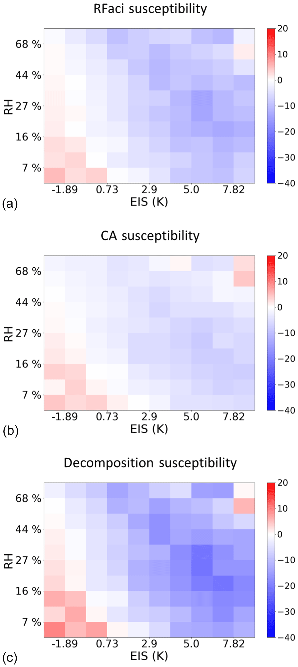
Figure 3Variations in the (a) RFaciwarm susceptibility, −5.26 Wm−2ln(AI)−1, (b) cloud adjustment susceptibility, −2.88 Wm−2ln(AI)−1, and (c) the sum of the two susceptibilities, i.e., the decomposed ERFaciwarm susceptibility, −8.22 Wm−2ln(AI)−1, with meteorological regimes defined by EIS and RH700.
3.3 Constrained by local meteorology
When further separated by meteorological regimes defined by stability and RH700 of the free atmosphere, the influence of the environment becomes clearer as strong variations in both the sign and magnitude of RFaciwarm and CAwarm with environmental regime are evident (Fig. 3). Both the RFaciwarm and cloud adjustment susceptibilities show warming responses in the most unstable, driest regimes. This is likely due to both the albedo and cloud extent being heavily influenced by entrainment-evaporation feedbacks (Small et al., 2009; Christensen et al., 2014). λCA shows a warming in the highest-humidity, most stable regimes, which may reflect cloud breakup processes like the stratocumulus to cumulus transition.
The total decomposed ERFaciwarm susceptibility, given by the sum of both the RFaciwarm and cloud adjustments within each individual stability and humidity regime, exhibits strong regime-specific susceptibilities, demonstrating the importance of understanding the total warm-cloud radiative response to aerosol with consideration of the environment. Constraints on meteorology allow us consider how meteorology influences the cloud response to aerosol. Without these constraints, any derived susceptibilities could be attributed environmental responses. While cloud darkening occurs in only the most unstable regime ( K), λCA continues to show a warming response in moderately neutral environments (∼2 K). This suggests that the instantaneous response (RFaci) is more sensitive to local meteorology than the slower cloud adjustments.
The dominant cooling of λRFaci and λCA in stable regimes illustrates the potential of a stable inversion to strengthen ACIs. The peak cooling of λCA occurs in a relatively dry atmosphere ∼27 % RH700. In this environment, the cloud extent rapidly increases as a response to aerosol; however the cloud is topped by a strong, stable inversion that prohibits much of an deepening of the cloud, perhaps instigating the effect to push horizontally rather than vertically (Christensen and Stephens, 2011). λRFaci peaks in stable but comparatively more moist environments where entrainment of moist air from the free atmosphere promotes activation of all available aerosol to CCN, rapidly increasing the albedo. This response may be similar to other regions where trade cumuli form and the FA is relatively moist (Koren et al., 2014).
Finally, while λRFaci shows less variation in sign, it exhibits more variation in magnitude between meteorological regimes indicating the importance of accounting for meteorological influences in order to capture this specific environmental regime dependence. It is possible that with additional constraints, understanding how other components of the meteorology is affecting these terms would become more clear. It is also possible λRFaci is impacted by some semidirect effects by smoke aerosol, which would lead to a cloud dimming and positive susceptibility. Semidirect effects are not accounted for by our methodology; however aerosol within the cloud layer could lead to cloud breakup processes, a dimmer albedo, and changes to the local environment by the absorbing aerosol.
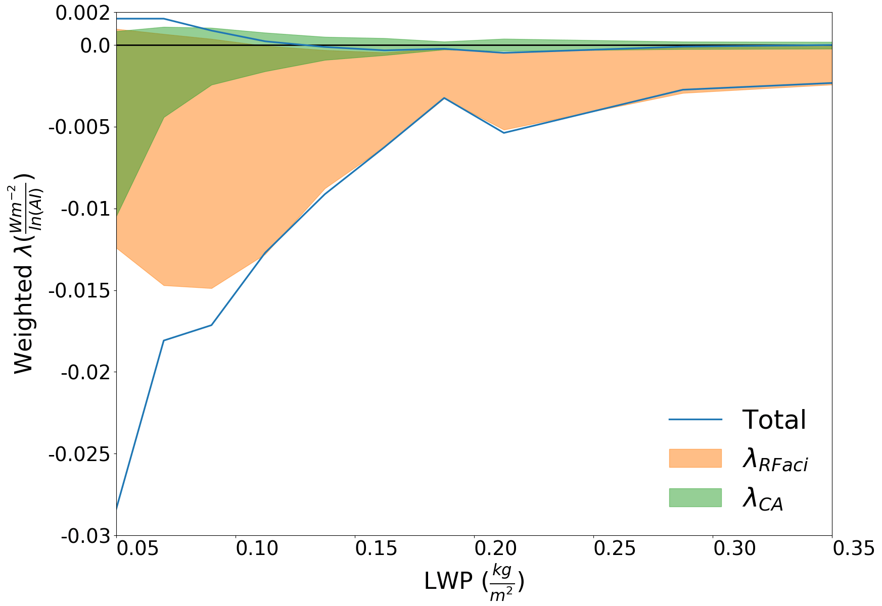
Figure 410 % to 90 % range of the decomposition for 11 cloud states when found within 100 environmental regimes of EIS and RH700. The RFaciwarm (orange fill, λRFaci) and cloud adjustment susceptibilities (green fill, λCA) total −4.18 Wm−2ln(AI)−1 and −1.26 Wm−2ln(AI)−1, respectively. The sum of the two from 10 to 90 percentiles, the decomposed susceptibility (blue line), totals −5.45 Wm−2ln(AI)−1.
3.4 Constraints on cloud state and local meteorology
As seen in Figs. 2 and 3, the susceptibility of each component of the ERFaciwarm varies with both cloud state and environmental regime. Therefore, when calculating each component of the ERFaciwarm, both the meteorology and LWP must be accounted for. To accomplish this, the RFaciwarm and CAwarm susceptibilities are found with constraints on both the LWP and environment (Fig. 4). The shaded region of Fig. 4 delineates the 10 % to 90 % range within each of the 11 cloud states of the susceptibility when further separated by the 100 environmental regimes used in Fig. 3. Unlike in Figs. 2 and 3, λ is weighted by frequency of occurrence within each environmental state. This illustrates how the magnitude and sign of each susceptibility can vary by environmental regime even when LWP is held approximately constant. The weighted and summed susceptibility is −5.45 Wm−2ln(AI)−1 with constraints on LWP, stability, and RH700 globally. This is slightly smaller than the susceptibility found in DL19; however, that susceptibility took into account all changes in warm-cloud CRE to aerosol, while our decomposition only accounts for the two largest effects, the albedo and cloud extent susceptibilities to aerosol. The lowest-LWP clouds (≤0.1 kgm−2) not only contribute most to the net susceptibility due to their abundance but also exhibit the widest range in susceptibilities across different meteorological states.
The two components exhibit different behavior in terms of susceptibility to cloud state (defined here by LWP). The cloud adjustment susceptibility is largest for the lowest LWPs, while the RFaciwarm susceptibility peaks around 0.06 kgm−2 and gradually declines. This may represent a “sweet spot” of cloud albedo susceptibility. Up to 0.1 kgm−2, aerosol are easily activated, and there are few processes beyond entrainment and activation to reduce the concentration within the cloud layer. Beyond 0.1 kgm−2, where the RFaciwarm begins to decrease, the cloud may be influenced by precipitation formation, reducing the λRFaci within each environmental regime.
λCA decreases in magnitude with LWP. Higher-LWP clouds, independent of the environment, may be less susceptible to lifetime effects, as was seen in Fig. 2. Precipitation suppression, the main driver of cloud adjustments, becomes less likely as LWP increases (Fan et al., 2016; Sorooshian et al., 2009). The thinnest and smallest clouds may have the largest potential to experience a enhancement effect.
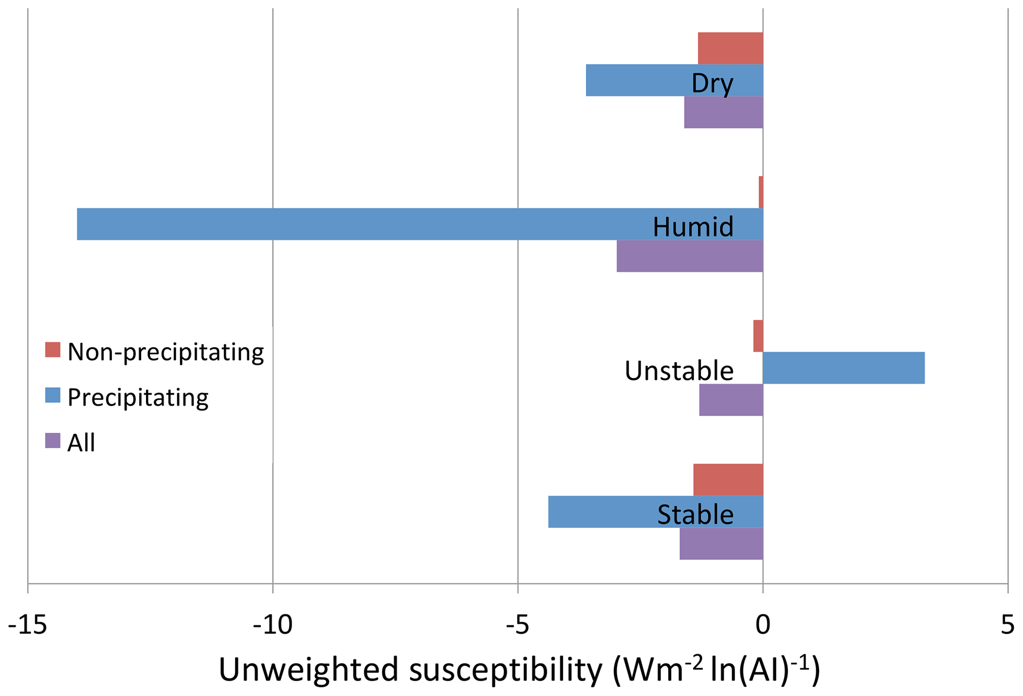
Figure 5Globally summed and relatively weighted susceptibilities for different conditions when found within regimes of EIS, RH, and LWP on a regional basis.
3.5 Impact of precipitation and environment on susceptibility
Precipitation formation within the cloud and the environment surrounding modulate the susceptibility. When weighted by the relative frequency of occurrence, rather than overall frequency of occurrence, the susceptibility of precipitating clouds is shown to be much higher in some environments than non-precipitating clouds (Fig. 5). Precipitating clouds in humid environments especially, defined as having a RH700 > 44 %, have a much greater susceptibility than any other regime of clouds. Unstable clouds show a reduced susceptibility in all cases, with precipitating clouds showing a warming effect in these environments, while non-precipitating clouds experience an extremely damped cooling effect. Unsurprisingly, in dry environments and stable environments, precipitation does less to magnify the susceptibility, and the difference between precipitating and non-precipitating susceptibilities is reduced.
Precipitating clouds reduce the amount of aerosol available to interact with warm clouds through wet scavenging, yet they still may induce several other processes within the cloud that stimulate a response Gryspeerdt et al.. These include stabilizing the boundary layer through virga and increasing the EIS and therefore susceptibility (Fig. 3). Precipitation formation within the cloud induces vertical motion and mixing of the cloud layer, increasing turbulence and mixing of the layer, which may increase activation of aerosol and therefore the response of the cloud. Further work must be done to resolve how and to what magnitude precipitation alters the warm-cloud radiative susceptibility to aerosol.
3.6 Contribution of RFaci and cloud adjustments to global ERFaci
With these considerations in mind, the sum of the RFaciwarm and CA, or the decomposed ERFaciwarm as we will refer to it, is Wm−2, found using Eq. (9) (Fig. 7). The components of the ERFaciwarm, i.e., the RFaciwarm and cloud adjustments, are found using Eqs. (5) and (7) and shown in Fig. 6. The ERFaciwarm from Fig. 1 is slightly larger in magnitude than the decomposed ERFaciwarm. Overall, their regional variations and magnitudes are extremely similar, suggesting the linear decomposition captures a majority of the ERFaciwarm. The southern oceans dominate the decomposed ERFaciwarm, as is expected based on the susceptibilities. The difference in overall magnitude stems from a stronger dimming effect evaluated in the decomposed ERFaciwarm (Fig. 6). In the decomposed ERFaciwarm, more regions experience a decrease in CRE with increasing AI compared to the ERFaciwarm. This may be due to the definition of the decomposed ERFaciwarm that allows either the RFaciwarm or CAwarm to reduce cooling.
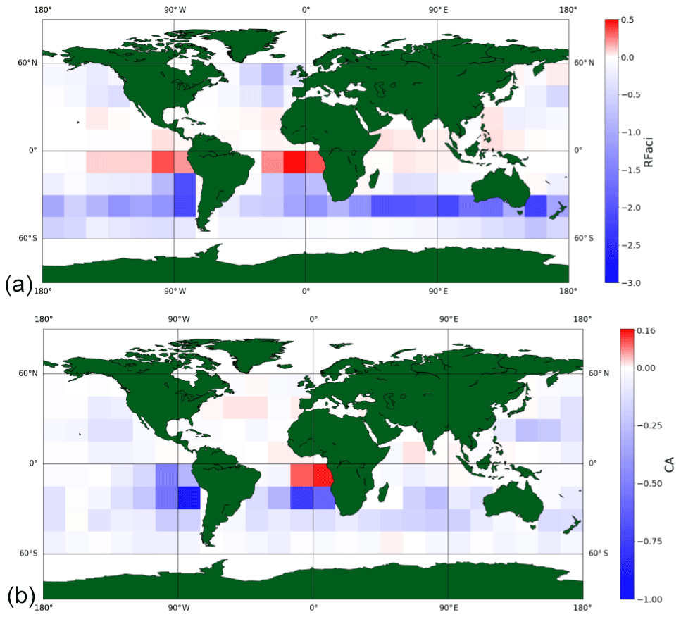
Figure 6(a) The radiative forcing due to aerosol–cloud interactions (RFaci) ( Wm−2) and (b) cloud adjustments ( Wm−2) found on a regional basis with constraints on LWP, EIS, and RH700 without weighting by area. Note the color bar for (b) CAwarm is 1∕3 of the magnitude of (a) RFaciwarm.
A reduced albedo, or positive RFaci, has been noted by other observation-based studies before (Chen et al., 2012). A positive RFaciwarm can be caused by multiple processes. A semidirect effect, where non-activated aerosol acts to decrease the total albedo of the cloud in the case of smoke, reduces the CRE of the cloud and therefore the RFaciwarm (Johnson et al., 2004). A decrease in the RFaciwarm may also be due to any changes to the distribution of liquid water throughout the cloud layer. In certain environmental conditions, an increase in aerosol may lead to sedimentation within the cloud throughout the entrainment zone, which could decrease the cloud albedo and therefore CRE (Ackerman et al., 2004). If these two effects combined under the “perfect storm” of aerosol and environmental conditions, the RFaciwarm would have a large, positive effect.
The cloud adjustment term likewise undergoes a positive (damped cooling) response in certain regions. A reduced cloud fraction due to aerosol–cloud interactions has been noted before by others (Small et al., 2009; Gryspeerdt et al., 2016). Chen et al. (2014) noted a decrease in LWP due to an increase in AI in their observationally based study, while other studies have indicated the LWP response and therefore cloud fraction response can be either positive or negative (Gryspeerdt et al., 2019). Any process that alters the cloud's liquid water path, such as evaporation–entrainment, may lead to a decrease in cloud fraction given certain environmental conditions.
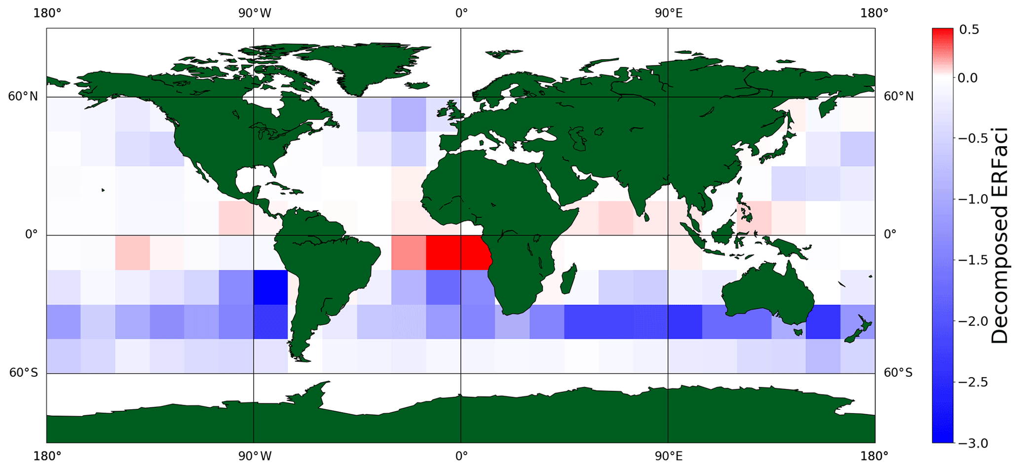
Figure 7The ERFaciwarm found as a sum of the RFaciwarm and cloud adjustments (Fig. 6) with constraints on the LWP, EIS, and RH700 on a regional basis (−0.26 Wm−2) without areal weighting.
The discrepancy between the two estimates of ERFaciwarm (0.065 Wm−2) may be cloud adjustment effects or covariance between RFaciwarm and CAwarm not captured by the simple regression employed here. The error between the two lies well within the bounds of error of both estimates (±0.16 and ±0.15). While cloud extent changes are the dominant cloud adjustment effect, changes in liquid water path due to precipitation suppression will have an impact on the radiative forcing as well. Future work on understanding and evaluating the ERFaciwarm must include other cloud adjustments and explicitly account for covariance between the RFaciwarm and cloud adjustments. Although they occur on different timescales, the RFaciwarm could be thought of as reactive to cloud adjustments. So while the cloud adjustment process may take hours, an albedo adjustment occurs simultaneously.
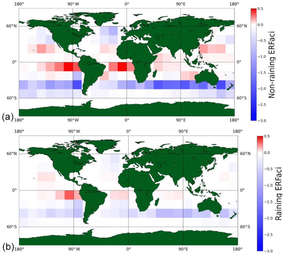
Figure 8The decomposed effective radiative forcing due to aerosol–cloud interactions found as a sum of its components on a regional scale within regimes of EIS, RH, and LWP for (a) non-raining clouds (−0.147 Wm−2) and (b) raining clouds (−0.06 Wm−2).
3.7 Regional variation due to precipitation
Figure 5 clearly demonstrates that precipitation plays a leading role in modulating the magnitude of aerosol–cloud interactions and their resultant forcing. The contribution of precipitating and non-precipitating clouds to the ERFaciwarm is presented in Fig. 8. Precipitation has a large impact on both the RFaciwarm and warm-cloud adjustment processes, indicated by the difference in global magnitudes between the two ERFaciwarm when separated by precipitation (−0.21 Wm−2) and not separated by precipitation (Fig. 7 −0.26 Wm−2). Precipitating clouds exhibit different microphysical processes and therefore pathways of aerosol–cloud interactions that lead to an increased susceptibility (−43.0 Wm−2ln(AI)−1 vs. −30.0 Wm−2ln(AI)−1 weighed individually). However, on average only ∼30 % of warm clouds observed by CloudSat are precipitating, leading to a smaller net contribution to the total ERFaciwarm shown in Fig. 8. If in future climates, warm clouds rain more frequently, it is possible that the decomposed ERFaciwarm could increase due to precipitating clouds higher susceptibilities, given the environmental conditions (EIS and RH) remain constant.
In regions where trade cumulus are more prevalent and the marine boundary layer is more unstable, precipitation clouds have the capacity to greatly decrease the cooling due to ERFaciwarm (Figs. 5, 8). However, this positive ERFaciwarm is balanced by their expansive cooling throughout the Southern Ocean. More regions experience a cooling due to ACIs when clouds are precipitating than not precipitating. Further, due to wet scavenging of aerosol, it is possible that precipitating clouds could reduce semidirect or direct effects and remove aerosol that could otherwise warm the atmosphere. The possible feedbacks or consequences of changes in precipitation require further research, especially since precipitation is heavily controlled by aerosol type as well as concentration.
The global distribution of the warm, marine cloud ERFaci and its components, the RFaciwarm and cloud adjustments, are found with constraints on cloud state and local meteorology following the methodology of DL19. The total effective radiative forcing due to aerosol–cloud interactions is Wm−2. The radiative forcing due to aerosol–cloud interactions is Wm−2. The forcing due to cloud adjustments from aerosol–cloud interactions is Wm−2. In all cases, constraining the environment and cloud state are found to be critical for reducing error in misrepresenting aerosol-environment effects as aerosol–cloud interactions. Our estimations of the ERFaciwarm, as a sum and/or single term, agrees with other estimates of the warm-cloud ERFaciwarm such as that of Chen et al., which estimated −0.46 Wm−2, and with Christensen et al., which estimated −0.36 Wm−2. The latter further showed liquid clouds dominate the ERFaciwarm over mixed-phase and ice-phase aerosol–cloud–radiation interactions. Thus changes in the warm-cloud susceptibility to aerosol perturbations could substantially alter the radiative balance due to the warm-cloud dominance of the ERFaciwarm.
Regionally, the ERFaciwarm derived from the linear decomposition into RFaciwarm and cloud adjustments agrees moderately well with that derived directly from the SW CRE, proving our method of decomposing the ERFaciwarm to the first-order components does capture the main effects adequately. Globally, the ERFaciwarm is dominated by the RFaciwarm; however the cloud adjustment term is found to contribute approx. one-fifth of the total forcing. The cloud adjustments vary regionally in sign and magnitude, meaning in some regions the two effects are additive, while in others they may cancel each other out. In the South Atlantic, both effects lead to a warming (positive) forcing as clouds both shrink and dim in this region, most likely due to the prevalence of a drier free atmosphere and unstable boundary layer in this region. In the tropical Pacific, clouds dim while the cloud extent swells, leading to an overall muted cooling effect. Regions like this where the two signals have opposing signals are prime examples of why a decomposition of the ERFaciwarm into its components is necessary. The muted signal in the tropical Pacific would most likely be attributed to offsetting reactions in the RFaciwarm and CAwarm, as this region shows a damped signal of ERFaciwarm, if not for the knowledge that the RFaciwarm and CAwarm have opposing responses in this region.
It is possible our simple methodology to evaluate cloud adjustments underestimates the possible forcing due to other adjustment processes or the possible covariance with the RFaciwarm. If the difference between the ERFaciwarm and the sum of the RFaciwarm and cloud adjustments is assumed to arise from the missing forcing from other adjustments, the total contribution of the CAwarm to the ERFaciwarm would increase to −0.11 Wm−2, or nearly a third, of the −0.32 Wm−2. This would be consistent with a recent estimate by Rosenfeld et al., which found the relationship between the total concentration of cloud droplets and cloud fraction, when constrained by LWP, still had a significant signal. Cloud adjustments are found to dominate over the RFaciwarm at the lowest liquid water paths. Thus in regions or climate conditions that support enhanced prevalence of thin clouds, the cloud adjustment term would increase at the expense of the RFaciwarm.
The Southern Hemisphere dominates the global ERFaciwarm due to ubiquitous marine stratocumulus in the South Pacific and South Atlantic. The Northern Hemisphere storm tracks region in the North Atlantic and marine stratocumulus off California exert approx. one-fifth of the magnitude of forcing observed from the pristine warm clouds of the Southern Hemisphere. Warm clouds in the Southern Hemisphere are predisposed to aerosol–cloud–radiation interactions.
Cloud adjustments and RFaciwarm varying regionally in sign and magnitudes implies that there are regions and conditions where the two components could effectively cancel each other out, thwarting short-term, observation-based attempts at discerning a noticeable change in cloud radiative effects due to aerosol. Moreover, the character of the clouds does not remain constant. Aerosol interactions that result in brighter clouds covering a smaller area or dimmer clouds covering a larger area represent important physical responses that may be masked by direct assessment of ERFaciwarm from CRE alone. In these regions especially, care should be taken in discerning which effect is dominating and to what magnitude.
All data used are publicly available. Satellite observations are available as stated in the acknowledgements. All CloudSat data are available from the CloudSat Data Processing Center (http://www.cloudsat.cira.colostate.edu; NASA, 2018a). MODIS, AMSR-E, and MERRA-2 Reanalysis data are available from the NASA Earth Data repository (https://earthdata.nasa.gov/; NASA, 2018b). SPRINTARS aerosol information is available at the SPRINTARS archive (https://sprintars.riam.kyushu-u.ac.jp/; Takemura, 2018).
AD performed all analysis, writing, and coding. TL'E helped with analysis and guided the discussion.
The authors declare that they have no conflict of interest.
This work was supported by NASA CloudSat/CALIPSO Science Team grant no. NNX13AQ32G and through the Jet Propulsion Laboratory, California Institute of Technology, CloudSat grant no. G-3969-1. Special thanks to Toshihiko Takemura at Kyushu University for the SPRINTARS modeled AI.
This research has been supported by the NASA (grant no. G-3969-1).
This paper was edited by Johannes Quaas and reviewed by two anonymous referees.
Ackerman, A. S., Kirkpatrick, M. P., Stevens, D. E., and Toon, O. B.: The impact of humidity above stratiform clouds on indirect aerosol climate forcing, Nature, 432, 1014, https://doi.org/10.1038/nature03174, 2004. a, b
Albrecht, B. A.: Aerosols, cloud microphysics, and fractional cloudiness, Science, 245, 1227–1230, 1989. a, b
Bony, S. and Dufresne, J.-L.: Marine boundary layer clouds at the heart of tropical cloud feedback uncertainties in climate models, Geophys. Res. Lett., 32, L20806, https://doi.org/10.1029/2005GL023851, 2005. a
Boucher, O., Randall, D., Artaxo, P., et al.: Clouds and aerosols, in: Climate change 2013: the physical science basis. Contribution of Working Group I to the Fifth Assessment Report of the Intergovernmental Panel on Climate Change, Cambridge University Press, 571–657, 2013. a, b
Carslaw, K. S., Lee, L. A., Reddington, C. L., Pringle, K. J., Rap, A., Forster, P. M., Mann, G. W., Spracklen, D. V., Woodhouse, M. T., Regayre, L. A., and Pierce, J. R.: Large contribution of natural aerosols to uncertainty in indirect forcing, Nature, 503, 67–71, https://doi.org/10.1038/nature12674, 2013. a, b
Carslaw, K. S., Gordon, H., Hamilton, D. S., Johnson, J. S., Regayre, L. A., Yoshioka, M., and Pringle, K. J.: Aerosols in the Pre-industrial Atmosphere, Current Climate Change Reports, 3, 1–15, https://doi.org/10.1007/s40641-017-0061-2, 2017. a
Chen, Y. and Penner, J. E.: Uncertainty analysis for estimates of the first indirect aerosol effect, Atmos. Chem. Phys., 5, 2935–2948, https://doi.org/10.5194/acp-5-2935-2005, 2005. a, b
Chen, Y.-C., Christensen, M. W., Xue, L., Sorooshian, A., Stephens, G. L., Rasmussen, R. M., and Seinfeld, J. H.: Occurrence of lower cloud albedo in ship tracks, Atmos. Chem. Phys., 12, 8223–8235, https://doi.org/10.5194/acp-12-8223-2012, 2012. a
Chen, Y.-C., Christensen, M. W., Stephens, G. L., and Seinfeld, J. H.: Satellite-based estimate of global aerosol–cloud radiative forcing by marine warm clouds, Nat. Geosci., 7, 643–646, https://doi.org/10.1038/ngeo2214, 2014. a, b, c
Chen, Y.-C., Christensen, M. W., Diner, D. J., and Garay, M. J.: Aerosol-cloud interactions in ship tracks using Terra MODIS/MISR, J. Geophys. Res.-Atmos., 120, 2819–2833, 2015. a
Christensen, M., Suzuki, K., Zambri, B., and Stephens, G.: Ship track observations of a reduced shortwave aerosol indirect effect in mixed-phase clouds, Geophys. Res. Lett., 41, 6970–6977, 2014. a, b
Christensen, M. W. and Stephens, G. L.: Microphysical and macrophysical responses of marine stratocumulus polluted by underlying ships: Evidence of cloud deepening, J. Geophys. Res.-Atmos., 116, D03201, https://doi.org/10.1029/2010JD014638, 2011. a
Christensen, M. W., Chen, Y.-C., and Stephens, G. L.: Aerosol indirect effect dictated by liquid clouds, J. Geophys. Res.-Atmos., 121, 14636–14650, https://doi.org/10.1002/2016JD025245, 2016. a, b, c
Christensen, M. W., Neubauer, D., Poulsen, C. A., Thomas, G. E., McGarragh, G. R., Povey, A. C., Proud, S. R., and Grainger, R. G.: Unveiling aerosol–cloud interactions – Part 1: Cloud contamination in satellite products enhances the aerosol indirect forcing estimate, Atmos. Chem. Phys., 17, 13151–13164, https://doi.org/10.5194/acp-17-13151-2017, 2017 a
Cochrane, S. P., Schmidt, K. S., Chen, H., Pilewskie, P., Kittelman, S., Redemann, J., LeBlanc, S., Pistone, K., Kacenelenbogen, M., Segal Rozenhaimer, M., Shinozuka, Y., Flynn, C., Platnick, S., Meyer, K., Ferrare, R., Burton, S., Hostetler, C., Howell, S., Freitag, S., Dobracki, A., and Doherty, S.: Above-cloud aerosol radiative effects based on ORACLES 2016 and ORACLES 2017 aircraft experiments, Atmos. Meas. Tech., 12, 6505–6528, https://doi.org/10.5194/amt-12-6505-2019, 2019. a
Dagan, G., Koren, I., Altaratz, O., and Heiblum, R. H.: Aerosol effect on the evolution of the thermodynamic properties of warm convective cloud fields, Sci. Rep.-UK, 6, 38769, https://doi.org/10.1038/srep38769, 2016. a
Dagan, G., Koren, I., Altaratz, O., and Lehahn, Y.: Shallow convective cloud field lifetime as a key factor for evaluating aerosol effects, iScience, 10, 192–202, 2018. a
De Roode, S. R., Siebesma, A. P., Dal Gesso, S., Jonker, H. J., Schalkwijk, J., and Sival, J.: A mixed-layer model study of the stratocumulus response to changes in large-scale conditions, J. Adv. Model. Earth Sy., 6, 1256–1270, 2014. a
Douglas, A. and L'Ecuyer, T.: Quantifying variations in shortwave aerosol–cloud–radiation interactions using local meteorology and cloud state constraints, Atmos. Chem. Phys., 19, 6251–6268, https://doi.org/10.5194/acp-19-6251-2019, 2019. a, b
Douglas, A. R.: Understanding Warm Cloud Aerosol-cloud Interactions, MS thesis, University of Wisconsin, Madison, 2017. a, b
Fan, J., Wang, Y., Rosenfeld, D., and Liu, X.: Review of aerosol–cloud interactions: Mechanisms, significance, and challenges, J. Atmos. Sci.., 73, 4221–4252, 2016. a, b, c
Feingold, G.: Modeling of the first indirect effect: Analysis of measurement requirements, Geophys. Res. Lett., 30, 1997, https://doi.org/10.1029/2003GL017967, 2003. a
Feingold, G., McComiskey, A., Yamaguchi, T., Johnson, J. S., Carslaw, K. S., and Schmidt, K. S.: New approaches to quantifying aerosol influence on the cloud radiative effect, P. Natl. Acad. Sci. USA, 113, 5812–5819, 2016. a
Fiedler, S., Stevens, B., Gidden, M., Smith, S. J., Riahi, K., and van Vuuren, D.: First forcing estimates from the future CMIP6 scenarios of anthropogenic aerosol optical properties and an associated Twomey effect, Geosci. Model Dev., 12, 989–1007, https://doi.org/10.5194/gmd-12-989-2019, 2019. a
Gelaro, R., McCarty, W., Suarez, M. J., Todling, R., Molod, A., Takacs, L., Randles, C. A., Darmenov, A., Bosilovich, M. G., Reichle, R., Wargan, K., Coy, L., Cullather, R., Draper, C., Akella, S., Buchard, V., Conaty, A., da Silva, A. M., Gu, W., Kim, G. K., Koster, R., Lucchesi, R., Merkova, D., Nielson, J. E., Partyka, G., Pawson, S., Putnam, W., Reinecker, M., Schubert, S. D., Sienkiewicz, M., and Zhao, B.: The modern-era retrospective analysis for research and applications, version 2 (MERRA-2), J. Climate, 30, 5419–5454, 2017. a
Gettelman, A. and Sherwood, S.: Processes responsible for cloud feedback, Current Climate Change Reports, 2, 179–189, 2016. a
Goren, T. and Rosenfeld, D.: Decomposing aerosol cloud radiative effects into cloud cover, liquid water path and Twomey components in marine stratocumulus, Atmos. Res., 138, 378–393, 2014. a
Gryspeerdt, E. and Stier, P.: Regime-based analysis of aerosol-cloud interactions, Geophys. Res. Lett., 39, L21802, https://doi.org/10.1029/2012GL053221, 2012. a
Gryspeerdt, E., Stier, P., White, B. A., and Kipling, Z.: Wet scavenging limits the detection of aerosol effects on precipitation, Atmos. Chem. Phys., 15, 7557–7570, https://doi.org/10.5194/acp-15-7557-2015, 2015. a
Gryspeerdt, E., Quaas, J., and Bellouin, N.: Constraining the aerosol influence on cloud fraction, J. Geophys. Res.-Atmos., 121, 3566–3583, 2016. a
Gryspeerdt, E., Quaas, J., Ferrachat, S., Gettelman, A., Ghan, S., Lohmann, U., Morrison, H., Neubauer, D., Partridge, D. G., Stier, P., Takemura, T., Wang, H., Wang, M., and Zhang, K.: Constraining the instantaneous aerosol influence on cloud albedo, P. Natl. Acad. Sci. USA, 114, 4899–4904, 2017. a
Gryspeerdt, E., Goren, T., Sourdeval, O., Quaas, J., Mülmenstädt, J., Dipu, S., Unglaub, C., Gettelman, A., and Christensen, M.: Constraining the aerosol influence on cloud liquid water path, Atmos. Chem. Phys., 19, 5331–5347, https://doi.org/10.5194/acp-19-5331-2019, 2019. a, b, c, d, e
Hahn, C. and Warren, S.: A Gridded Climatology of Clouds over Land (1971–96) and Ocean (1954–97 from Surface Observations Worldwide, Tech. rep., Office of Biological and Environmental Research, Oak Ridge, Tennessee, 2007. a
Hamilton, D. S., Lee, L. A., Pringle, K. J., Reddington, C. L., Spracklen, D. V., and Carslaw, K. S.: Occurrence of pristine aerosol environments on a polluted planet, P. Natl. Acad. Sci. USA, 111, 18466–18471, 2014. a, b
Hasekamp, O. P., Gryspeerdt, E., and Quaas, J.: Analysis of polarimetric satellite measurements suggests stronger cooling due to aerosol-cloud interactions, Nat. Commun., 10, 1–7, 2019. a, b
Haynes, J. M., L'Ecuyer, T. S., Stephens, G. L., Miller, S. D., Mitrescu, C., Wood, N. B., and Tanelli, S.: Rainfall retrieval over the ocean with spaceborne W-band radar, J. Geophys. Res.-Atmos., 114, D00A22, https://doi.org/10.1029/2008JD009973, 2009. a, b
Henderson, D. S., L'Ecuyer, T., Stephens, G., Partain, P., and Sekiguchi, M.: A multisensor perspective on the radiative impacts of clouds and aerosols, J. Appl. Meteorol. Clim., 52, 853–871, 2013. a, b
Johnson, B., Shine, K., and Forster, P.: The semi-direct aerosol effect: Impact of absorbing aerosols on marine stratocumulus, Q. J. Roy. Meteorol. Soc., 130, 1407–1422, 2004. a
Koren, I., Dagan, G., and Altaratz, O.: From aerosol-limited to invigoration of warm convective clouds, Science, 344, 1143–1146, 2014. a, b
Lebsock, M. and Su, H.: Application of active spaceborne remote sensing for understanding biases between passive cloud water path retrievals, J. Geophys. Res.-Atmos., 119, 8962–8979, 2014. a
Lebsock, M. D., Stephens, G. L., and Kummerow, C.: Multisensor satellite observations of aerosol effects on warm clouds, J. Geophys. Res.-Atmos., 113, D15205, https://doi.org/10.1029/2008JD009876, 2008. a
L'Ecuyer, T. S. and Jiang, J. H.: Touring the atmosphere aboard the A-Train, in: AIP Conference Proceedings, American Institute of Physics, Fort Collins, Colorado, vol. 1401, 245–256, 2011. a
L'Ecuyer, T. S. and Stephens, G. L.: An estimation-based precipitation retrieval algorithm for attenuating radars, J. Appl. Meteorol., 41, 272–285, 2002. a
L'Ecuyer, T. S., Berg, W., Haynes, J., Lebsock, M., and Takemura, T.: Global observations of aerosol impacts on precipitation occurrence in warm maritime clouds, J. Geophys. Res.-Atmos., 114, D0921, https://doi.org/10.1029/2008JD011273, 2009. a
McCoy, D., Bender, F.-M., Mohrmann, J., Hartmann, D., Wood, R., and Grosvenor, D.: The global aerosol-cloud first indirect effect estimated using MODIS, MERRA, and AeroCom, J. Geophys. Res.-Atmos., 122, 1779–1796, 2017. a
McCoy, D. T., Field, P., Gordon, H., Elsaesser, G. S., and Grosvenor, D. P.: Untangling causality in midlatitude aerosol-cloud adjustments, Atmos. Chem. Phys. Discuss., in review, 2020. a
Michibata, T., Suzuki, K., Sato, Y., and Takemura, T.: The source of discrepancies in aerosol–cloud–precipitation interactions between GCM and A-Train retrievals, Atmos. Chem. Phys., 16, 15413–15424, https://doi.org/10.5194/acp-16-15413-2016, 2016. a
Mülmenstädt, J. and Feingold, G.: The radiative forcing of aerosol–cloud interactions in liquid clouds: wrestling and embracing uncertainty, Current Climate Change Reports, 4, 23–40, 2018. a
NASA: CloudSat Database, available at: http://www.cloudsat.cira.colostate.edu, last access: 1 November 2018a. a
NASA: NASA Earth Data, MODIS/AMSR-E/MERRA-2, available at: https://earthdata.nasa.gov/, last access: 1 November 2018b. a
Nishant, N. and Sherwood, S.: A Cloud-Resolving Model Study of Aerosol-Cloud Correlation in a Pristine Maritime Environment, Geophys. Res. Lett., 44, 5774–5781, https://doi.org/10.1002/2017GL073267, 2017. a
Parkinson, C. L.: Aqua: An Earth-observing satellite mission to examine water and other climate variables, IEEE T. Geosci. Remote, 41, 173–183, 2003. a
Penner, J. E., Xu, L., and Wang, M.: Satellite methods underestimate indirect climate forcing by aerosols, P. Natl. Acad. Sci. USA, 108, 13404–13408, 2011. a
Platnick, S. and Twomey, S.: Determining the susceptibility of cloud albedo to changes in droplet concentration with the Advanced Very High Resolution Radiometer, J. Appl. Meteorol., 33, 334–347, 1994. a, b
Ramanathan, V., Crutzen, P., Kiehl, J., and Rosenfeld, D.: Aerosols, climate, and the hydrological cycle, Science, 294, 2119–2124, 2001. a
Rosenfeld, D.: Aerosol-cloud interactions control of earth radiation and latent heat release budgets, in: Solar Variability and Planetary Climates, Springer, 149–157, 2006. a
Rosenfeld, D., Lohmann, U., Raga, G. B., O'Dowd, C. D., Kulmala, M., Fuzzi, S., Reissell, A., and Andreae, M. O.: Flood or drought: how do aerosols affect precipitation?, Science, 321, 1309–1313, 2008. a
Rosenfeld, D., Zhu, Y., Wang, M., Zheng, Y., Goren, T., and Yu, S.: Aerosol-driven droplet concentrations dominate coverage and water of oceanic low-level clouds, Science, 363, eaav0566, https://doi.org/10.1126/science.aav0566, 2019. a
Sandu, I. and Stevens, B.: On the factors modulating the stratocumulus to cumulus transitions, J. Atmos. Sci., 68, 1865–1881, 2011. a
Sassen, K., Wang, Z., and Liu, D.: Global distribution of cirrus clouds from CloudSat/Cloud-Aerosol lidar and infrared pathfinder satellite observations (CALIPSO) measurements, J. Geophys. Res.-Atmos., 113, D00A12, https://doi.org/10.1029/2008JD009972, 2008. a
Seinfeld, J. H., Bretherton, C., Carslaw, K. S., Coe, H., DeMott, P. J., Dunlea, E. J., Feingold, G., Ghan, S., Guenther, A. B., Kahn, R., et al.: Improving our fundamental understanding of the role of aerosol-cloud interactions in the climate system, P. Natl. Acad. Sci. USA, 113, 5781–5790, 2016. a, b
Slingo, A.: Sensitivity of the Earth's radiation budget to changes in low clouds, Nature, 343, 49–51, https://doi.org/10.1038/343049a0, 1990. a
Small, J. D., Chuang, P. Y., Feingold, G., and Jiang, H.: Can aerosol decrease cloud lifetime?, Geophys. Res. Lett., 36, L16806, https://doi.org/10.1029/2009GL038888, 2009. a, b, c
Sorooshian, A., Feingold, G., Lebsock, M. D., Jiang, H., and Stephens, G. L.: On the precipitation susceptibility of clouds to aerosol perturbations, Geophys. Res. Lett., 36, L13803, https://doi.org/10.1029/2009GL038993, 2009. a, b
Stephens, G., Winker, D., Pelon, J., Trepte, C., Vane, D., Yuhas, C., L’ecuyer, T., and Lebsock, M.: CloudSat and CALIPSO within the A-Train: Ten years of actively observing the Earth system, B. Am. Meteorol. Soc., 99, 569–581, 2018. a
Stephens, G. L.: Cloud feedbacks in the climate system: A critical review, J. Climate, 18, 237–273, 2005. a
Stephens, G. L. and Wood, N. B.: Properties of tropical convection observed by millimeter-wave radar systems, Mon. Weather Rev., 135, 821–842, 2007. a
Stevens, B.: On the growth of layers of nonprecipitating cumulus convection, J. Atmos. Sci., 64, 2916–2931, 2007. a
Stevens, B.: Aerosols: Uncertain then, irrelevant now, Nature, 503, 47–48, https://doi.org/10.1038/503047a, 2013. a
Stevens, B. and Feingold, G.: Untangling aerosol effects on clouds and precipitation in a buffered system, Nature, 461, 607–613, 2009. a, b, c, d, e
Stier, P.: Limitations of passive remote sensing to constrain global cloud condensation nuclei, Atmos. Chem. Phys., 16, 6595–6607, https://doi.org/10.5194/acp-16-6595-2016, 2016. a
Su, W., Loeb, N. G., Xu, K.-M., Schuster, G. L., and Eitzen, Z. A.: An estimate of aerosol indirect effect from satellite measurements with concurrent meteorological analysis, J. Geophys. Res.-Atmos., 115, D18219, https://doi.org/10.1029/2010JD013948, 2010. a
Takemura, T.: SPRINTARS Model Forecasts, available at: https://sprintars.riam.kyushu-u.ac.jp/, last access: 1 November 2018. a
Takemura, T., Okamoto, H., Maruyama, Y., Numaguti, A., Higurashi, A., and Nakajima, T.: Global three-dimensional simulation of aerosol optical thickness distribution of various origins, J. Geophys. Res.-Atmos., 105, 17853–17873, 2000. a, b
Takemura, T., Nozawa, T., Emori, S., Nakajima, T. Y., and Nakajima, T.: Simulation of climate response to aerosol direct and indirect effects with aerosol transport-radiation model, J. Geophys. Res.-Atmos., 110, D02202, https://doi.org/10.1029/2004JD005029 2005. a
Tanelli, S., Durden, S. L., Im, E., Pak, K. S., Reinke, D. G., Partain, P., Haynes, J. M., and Marchand, R. T.: CloudSat's cloud profiling radar after two years in orbit: Performance, calibration, and processing, IEEE T. Geosci. Remote, 46, 3560–3573, 2008. a
Twohy, C. H., Petters, M. D., Snider, J. R., Stevens, B., Tahnk, W., Wetzel, M., Russell, L., and Burnet, F.: Evaluation of the aerosol indirect effect in marine stratocumulus clouds: Droplet number, size, liquid water path, and radiative impact, J. Geophys. Res.-Atmos., 110, D08203, https://doi.org/10.1029/2004JD005116, 2005. a
Twomey, S.: The Influence of Pollution on the Shortwave Albedo of Clouds, J. Atmos. Sci., 34, 1149–1152, 1977. a, b, c
Wentz, F. J. and Meissner, T.: Supplement 1 algorithm theoretical basis document for AMSR-E ocean algorithms, NASA: Santa Rosa, CA, USA, 2007. a
Wood, R.: Stratocumulus clouds, Mon. Weather Rev., 140, 2373–2423, 2012. a, b
Wood, R. and Bretherton, C. S.: On the relationship between stratiform low cloud cover and lower-tropospheric stability, J. Climate, 19, 6425–6432, 2006. a, b