Model simulations of atmospheric methane (1997–2016) and their evaluation using NOAA and AGAGE surface and IAGOS-CARIBIC aircraft observations

Methane (CH₄) is an important greenhouse gas, and its atmospheric budget is determined by interacting sources and sinks in a dynamic global environment. Methane observations indicate that after almost a decade of stagnation, from 2006, a sudden and continuing global mixing ratio increase took place. We applied a general circulation model to simulate the global atmospheric budget, variability, and trends of methane for the period 1997–2016. Using interannually constant CH₄ a priori emissions from 11 biogenic and fossil source categories, the model results are compared with observations from 17 Advanced Global Atmospheric Gases Experiment (AGAGE) and National Oceanic and Atmospheric Administration (NOAA) surface stations and intercontinental Civil Aircraft for the Regular observation of the atmosphere Based on an Instrumented Container (CARIBIC) flights, with > 4800 CH₄ samples, gathered on > 320 flights in the upper troposphere and lowermost stratosphere.

Based on a simple optimization procedure, methane emission categories have been scaled to reduce discrepancies with the observational data for the period 1997–2006. With this approach, the all-station mean dry air mole fraction of 1780 nmol mol⁻¹ could be improved from an a priori root mean square deviation (RMSD) of 1.31 % to just 0.61 %, associated with a coefficient of determination (R²) of 0.79. The simulated a priori interhemispheric difference of 143.12 nmol mol⁻¹ was improved to 131.28 nmol mol⁻¹, which matched the observations quite well (130.82 nmol mol⁻¹).

Analogously, aircraft measurements were reproduced well, with a global RMSD of 1.1 % for the measurements before 2007, with even better results on a regional level (e.g., over India, with an RMSD of 0.98 % and R²=0.65). With regard to emission optimization, this implied a 30.2 Tg CH₄ yr⁻¹ reduction in predominantly fossil-fuel-related emissions and a 28.7 Tg CH₄ yr⁻¹ increase of biogenic sources.

With the same methodology, the CH₄ growth that started in 2007 and continued almost linearly through 2013 was investigated, exploring the contributions by four potential causes, namely biogenic emissions from tropical wetlands, from agriculture including ruminant animals, and from rice cultivation, and anthropogenic emissions (fossil fuel sources, e.g., shale gas fracking) in North America. The optimization procedure adopted in this work showed that an increase in emissions from shale gas (7.67 Tg yr⁻¹), rice cultivation (7.15 Tg yr⁻¹), and tropical wetlands (0.58 Tg yr⁻¹) for the period 2006–2013 leads to an optimal agreement (i.e., lowest RMSD) between model results and observations.

1 Introduction

The greenhouse gas methane (CH₄) is emitted into the atmosphere by various natural and anthropogenic sources, and is removed by photochemical reactions and to a small extent through oxidation by methanotrophic bacteria in soils (Dlugokencky et al., 2011). The tropospheric mean lifetime of CH₄ due to oxidation by OH has been estimated to be 8–9 years (Lelieveld et al., 2016) and its concentration has been growing by about 1 % yr⁻¹ since the beginning of the Anthropocene in the 19th century (Crutzen, 2002; Ciais et al., 2013).

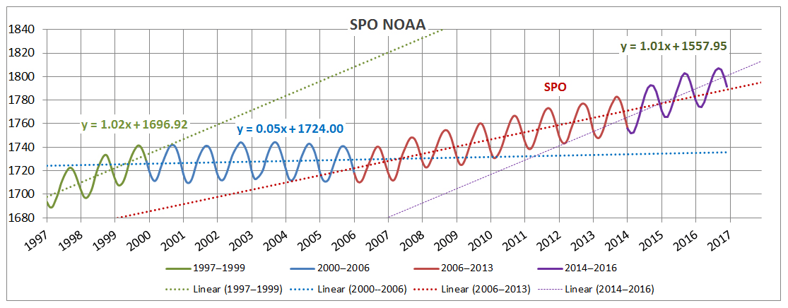
Figure 1 Development of monthly mean CH₄ mixing ratios (nmol mol⁻¹) at the NOAA observation site at the South Pole (SPO, 90^∘ S) over the years 1997–2016, the period considered in this modeling study.

The resulting factor of 2.5 increase in the global abundance of atmospheric methane (CH₄) starting from 1750 contributes 0.5 Wm⁻² to the direct radiative forcing by long-lived greenhouse gases (in total 2.8 Wm⁻² in 2009), while its role in atmospheric chemistry adds another approximately 0.2 Wm⁻² of indirect radiative forcing (Lelieveld et al., 1998; Dlugokencky et al., 2011). Etminan et al. (2016) presented new calculations including the impact of shortwave radiation absorption and found that the 1750–2011 direct radiative forcing is significantly higher (0.6 Wm⁻²) compared to that applied in the Intergovernmental Panel on Climate Change (IPCC) 2013 assessment. After the strong upward CH₄ trend starting from the 1960s, by the end of the 1990s the increase had slowed until sources and sinks balanced for about 8 years, while in 2007 the CH₄ increase resumed unexpectedly (Bergamaschi et al., 2013). Figure 1 demonstrates the development of CH₄ mixing ratios at the National Oceanic and Atmospheric Administration (NOAA) observation site at the South Pole (SPO, 90^∘ S) over the years 1997–2016, the period considered in this modeling study. Please notice the period without a trend from 2000 to 2006 and the one with a positive trend afterwards, which increases after 2014.

The resumed upward trend after 2007 (Dlugokencky et al., 2009; Rigby et al., 2008; IPCC, 2014) is not fully understood (Nisbet et al., 2016; Mikaloff-Fletcher and Schaefer, 2019), and causes of the trend changes have been subject of a number of studies, in part with contradictory results, highlighting the complexity of the processes that control atmospheric methane in the Anthropocene. Data analysis (Nisbet et al., 2016; Worden et al., 2017) and inverse modeling studies (Bergamaschi et al., 2013) indicate that global emissions since 2007 were about 15 to 25 Tg CH₄ yr⁻¹ higher than in preceding years, possibly caused by increasing tropical wetland emissions and anthropogenic pollution in midlatitudes of the Northern Hemisphere. Hausmann et al. (2016), using methane and ethane column measurements, concluded that the CH₄ increase that started in 2007 needs to be attributed for 18 %–73 % (depending on assumed ethane/methane source ratios) to thermogenic methane. Further, Helmig et al. (2016) suggested a large contribution of US oil and natural gas production to the increased emissions, with hydraulic shale gas fracturing as a potentially growing methane source (FracFocus, 2016). For instance, in Utah, 6 % to 12 % of the natural gas produced might have locally escaped into the atmosphere (Karion et al., 2013; Helmig et al., 2016).

On the other hand, Schwietzke et al. (2016) showed that overall fossil sources have decreased during the last decades due to industrial efficiency improvements, and Schaefer at al. (2016), based on ¹³C∕¹²C isotope ratio analyses for 2007–2011, concluded that fossil-fuel-related emissions are a minor contributor to the renewed methane increase, compared to tropical wetlands and agriculture. Nisbet et al. (2016) stated that “since 2007 δ¹³C−CH₄ (a measure of the ¹³C∕¹²C isotope ratio in methane) has shifted to significantly more negative values suggesting that the methane rise was dominated by increases in biogenic methane emissions, particularly in the tropics, for example, from expansion of tropical wetlands in years with strongly positive rainfall anomalies or emissions from increased agricultural sources such as ruminants and rice paddies”. Similarly, Saunois et al. (2016) concluded that agricultural activities are responsible for the atmospheric growth in the past decade and mentioned that “wetland emissions were estimated to be mostly unchanged between 2006 and 2012”. It must be stressed that the suggested increase in biogenic emissions raises concern about the contribution from rice production relative to wetland emissions. The latter, in fact, are higher in the Southern Hemisphere, whereas remote sensing shows that CH₄ mainly increased in the northern tropics and subtropics (Houweling et al., 2014). Furthermore, tropical wetlands match the post-2006 δ¹³C-CH₄ perturbation not as well as rice cultivation and C3-fed ruminants (Schaefer et al., 2016). The reason for the increase in methane starting from 2007 is therefore not established and debated in the scientific community.

In this work, we investigate CH₄ mixing ratios and their changes over the past two decades via numerical simulations and a large number of observations. The numerical model (the ECHAM/MESSy Atmospheric Chemistry model; EMAC), which accounts for atmospheric dynamical and chemical processes such as transport, dispersion, and chemistry of atmospheric trace constituents, has been evaluated based on CH₄ measurements at surface stations, i.e., data from NOAA (Dlugokencky et al., 2018) and Advanced Global Atmospheric Gases Experiment (AGAGE) (Prinn et al., 2016) and CH₄ data collected by the CARIBIC (Civil Aircraft for the Regular observation of the atmosphere Based on an Instrumented Container) passenger aircraft (Brenninkmeijer et al., 2007). The observational datasets are used to improve the model simulation of the methane mixing ratios and to test alternative sources for the post-2007 trend. The paper is organized as follows: in Sects. 2 and 3, the model setup and the observational datasets are presented, respectively. In Sect. 4, results from the numerical simulation of the period 1997–2007 are presented together with the emissions improvements, while in Sect. 5, the numerical model is used to test possible causes of the increased methane trends after 2007. The conclusions and outlook are followed by a summary of all abbreviations in the “Abbreviations” table.

2 Model setup

2.1 The EMAC numerical model

The EMAC model is a chemistry and climate simulation system that includes submodels describing tropospheric and middle-atmosphere processes and their interaction with oceans, land, and human influences. The Modular Earth Submodel System (MESSy; https://www.messy-interface.org, last access: 27 April 2020) results from a multi-institutional project providing a strategy for developing comprehensive Earth system models (ESMs) with flexible levels of complexity. MESSy describes atmospheric chemistry and meteorological processes in a modular framework, following strict coding standards. The submodels in EMAC have been coupled to the fifth-generation European Centre HAMburg general circulation model (ECHAM5; Röckner et al., 2006), of which the coding has been optimized for this purpose (Jöckel et al., 2006, 2010).

The extended EMAC model (version 2.50) at T106L90MA resolution was used to simulate the global methane budget, in part because some of the analyzed data were collected in the tropopause region and lower stratosphere, which provides a new perspective and additional model constraints compared to previous work. A triangular truncation at wavenumber 106 for the spectral core of ECHAM5 corresponds to a $\sim \mathrm{1.1}{}^{\circ }\times \mathrm{1.1}{}^{\circ }$ horizontal quadratic Gaussian grid spacing near the Equator, and 90 levels on a hybrid-pressure grid in the vertical direction span from the Earth's surface to 0.01 hPa pressure altitude (∼80 km, the middle of the uppermost layer). The vertical resolution near the tropopause is about 500 m. Numerical stability criteria require an integration time step of 1–2 min. With regard to model dynamics, we applied a weak “nudging” towards realistic meteorology over the period of interest, more specifically by Newtonian relaxation of the four prognostic model variables temperature, divergence, vorticity, and the logarithm of surface pressure towards ERA-Interim data (Dee et al., 2011) of the European Centre for Medium-Range Weather Forecasts (ECMWF).

Apart from the prescribed sea surface temperature (SST), the sea-ice concentration (SCI), and the nudged surface pressure, the nudging method is applied in the free troposphere only, tapering off towards the surface and the tropopause, so that stratospheric dynamics are calculated freely, and possible inconsistencies between the boundary layer representations of the ECMWF and ECHAM models are avoided. Further, in the free troposphere, the nudging is weak enough to not disturb the self-consistent model physics, while this approach allows a direct comparison of the model output with measurement data (without constraining the model physics) and therefore offers an efficient model evaluation.

The EMAC submodels used in this study include “CH4” (Frank, 2018) which is tailored for stratospheric and tropospheric methane chemistry and solves the ordinary differential equations describing the oxidation of methane by OH, O(¹D), Cl, and photolysis. The feedback to the hydrological cycle by modification of the specific humidity is optional in “CH4” and was switched off for the simulations of the present study. The submodels “SCOUT” and “S4D” enable online sampling of model parameters such as tracer mixing ratios at selected observation sites as well as along aircraft flight routes (https://www.messy-interface.org/, last access: 27 April 2020; see “MESSy Submodels” and Jöckel et al., 2010).

It is important to underline that a single simulation was performed with the model covering the 1997–2017 period. However, as described in Sect. 2.2.4, the emission optimizations were performed for two different time spans of the model simulation, i.e., for the period 1997–2006 and for the period 2006–2013.

Table 1 Methane emissions from eleven sectors: annual amounts and lifetime τ.

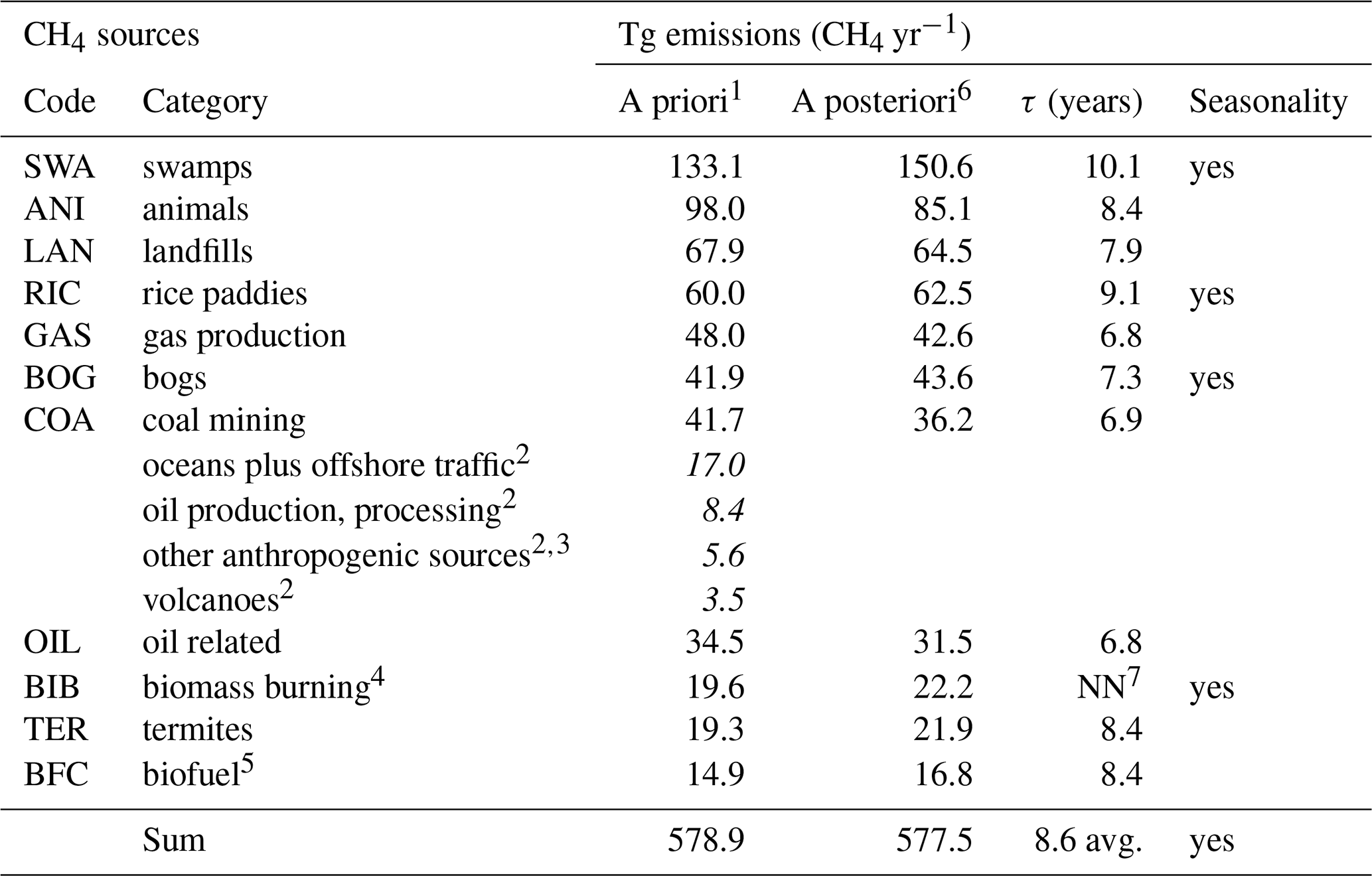
¹ Methane emissions (Houweling et al., 2006) for EMAC model input (1997–2006; no-trend period). ² Items merged in one category “oil related” by ¹ (numbers in italics). ³ All EDGAR emission classes related to the use of fossil fuels such as residential heating, onshore traffic, and industry. ⁴ GFEDv4s statistics (Randerson et al., 2018). ⁵ EDGARv2.0 database (Olivier et al., 2001/2002). ⁶ Rescaled with respect to minimal station observation to model simulation root mean square deviation (RMSD). ⁷ Interannual biomass burning variable.

2.2 Methane sources and sinks

2.2.1 Methane a priori emissions

In our study, 11 emission categories are considered in the model: swamps or wetlands (SWA), animals (ANI), landfills (LAN), rice paddies (RIC), gas production (GAS), bogs (BOGS), coal mining (COA), oil-related emissions, including minor natural ones from oceans, volcanoes and offshore traffic (OIL), biomass burning (BIB), termites (TER), and biofuel combustion (BFC).

These emissions (with the exception of BIB) do not follow any interannual variability, while only emissions from bogs, rice fields, swamps, and biomass burning are subject to seasonal variability. In Table 1, the a priori emissions from these emissions are listed, with a total amount of 580 Tg CH₄ yr⁻¹. These emissions have been applied for the entire simulation period (1997–2016).

The a priori emission fields of anthropogenic and natural methane sources are based on the Global Atmospheric Methane Synthesis (GAMeS), a GAIM/IGBP (http://gaim.unh.edu/, last access: 27 April 2020) initiative to develop a process-based understanding of the global atmospheric methane budget for use in predicting future atmospheric methane burdens. Emission data for this initiative have been used for the model setup described here. Natural wetland emissions are based on Walter et al. (2000), fossil sources based on EDGARv2.0, and remaining sources as compiled by Fung et al. (1991). Processes with similar isotopic characteristics are aggregated into one group. Oil-related sources, for example, comprise mining and processing of crude fuel and all emission classes related to the use of fossil fuel such as residential heating, on/offshore traffic, industry, etc., and also include an estimate of volcanoes (Houweling et al., 1999). Given that methane emissions from boreal/arctic wetlands are quite uncertain, it is reasonable to assume that this source category accounts for permafrost decomposition emissions as well.

The biomass burning of the GAMeS dataset is replaced by the GFEDv4s statistics (Randerson et al., 2018) and is vertically distributed up to 3000 m altitude and higher according to a profile suggested in EDGAR3.2ft (Van Aardenne et al., 2005). The GFEDv4 biomass burning statistics include agricultural waste burning events. Biomass burning emissions are interannually variable, and the 1997 emission was 2.4 times as high as the 1998–2015 average (Fig. S1c in the Supplement). Further, the biofuel combustion emissions are from the EDGARv2.0 database (Olivier et al., 2001/2002).

About 60 % of the total emissions of 580 Tg yr⁻¹ are caused by human activities; the remainder is from natural sources. At northern middle and high latitudes, methane sources predominantly comprise animals (ruminants), bogs, gas and coal production, transmission and use, landfills, and boreal biomass fires. Tropical wetlands (partly in the subtropics) are the world's largest (natural) source of methane together with animals. Minor tropical anthropogenic input is from biofuel combustion.

The horizontal resolution of all methane fluxes is $\mathrm{1}{}^{\circ }\times \mathrm{1}{}^{\circ }$ and, except for interannual differences in the ∼20 Tg yr⁻¹ biomass burning, are assumed to be interannually constant in a reference simulation for the full period (1997–2016). Further plots are provided in the Supplement, such as Fig. S1, which depicts the total emission distribution in grams (CH₄) m⁻² month⁻¹ for January (a) and July (b), in logarithmic scale for better representation, to illustrate seasonal CH₄ changes.

The additional emission sources tested as possible causes in the methane rise period after 2006 are based on enhanced emissions from tropical wetlands (scenario TRO), from agriculture including ruminant animals (ANI) and rice cultivation (RIC), and new emissions from shale gas drilling called fracking (SHA). The ANI and RIC emissions are based on the existing emission distribution, while the TRO emissions are equal to the wetland (or swamp, SWA) sector but restricted to the tropical belt. Finally, the SHA distribution map was produced thanks to the publicly available database maintained by the national hydraulic fracturing chemical registry (FracFocus, 2016). Figure S2 depicts the geographical distribution of the global CH₄ mixing ratios near the surface, logarithmically scaled for better visibility, marking the respective hypothetical sources. At the same intensity, SHA and RIC emissions are more spatially concentrated compared to TRO and ANI. Large areas of ANI cover the same region over India as RIC, which may be an uncertainty factor in the source attribution analysis, although the seasonal behavior of RIC provides clues to distinguish between them. The stronger vertical transport intensity of TRO compared to SHA, leading to reduced altitude gradients (Fig. S3) is related to the proximity to the intertropical convergence zone (ITCZ).

2.2.2 Methane uptake by soils

A small (6.6 % in this study) removal process of methane is its oxidation by methanotrophic bacteria in soils (Dlugokencky et al., 2011). The MESSy submodel “DDEP” simulates dry deposition of gas phase tracers and aerosols (Kerkweg et al., 2006). For our CH₄ budget modeling, the deposition flux was derived for a fixed atmospheric-methane mixing ratio of 1800 nmol mol⁻¹ (Spahni et al., 2011; Ridgwell et al., 1999) and is scaled accordingly. The deposition has a pronounced seasonal cycle in phase with the wetland emissions and depends on soil temperature, moisture content, and the land cultivation fraction, and varies from 2.4 Tg in January to 4.0 Tg in July.

2.3 Methane chemical removal

The chemical removal process of CH₄ is photo-oxidation, predominantly by hydroxyl (OH) radicals. In addition to the reaction with OH in the troposphere and stratosphere, there are minor oxidation reactions with atomic chlorine (Cl) in the marine boundary layer and the stratosphere and with electronically excited oxygen atoms (O(¹D)) in the stratosphere (Lelieveld et al., 1998; Dlugokencky et al., 2011). In EMAC, the methane photochemical reaction system is numerically solved by the submodel “CH4”. Global distributions of OH, Cl, and O(¹D) have been precalculated from a model simulation that was evaluated previously (see simulation S1; Jöckel et al., 2006), therefore providing internally consistent oxidation fields for the model transport and chemistry of precursors. With this approach, we neglect interannual changes in global OH, which are assumed to be small (Nisbet et al., 2016). Potential changes in the removal rate of methane by the OH radical have not been seen in other tracers of atmospheric chemistry, e.g., methyl chloroform (CH₃CCl₃) (Montzka et al., 2011; Lelieveld et al., 2016) and do not appear to explain short-term variations in methane. Nevertheless, Turner et al. (2017) found that a combination of decreasing methane emissions overlaid by a simultaneous reduction in OH concentration (the primary sink) could have caused the renewed growth in atmospheric methane. However, they could not exclude rising-methane emissions under time-invariant OH concentrations as a consistent solution to fit the (rising) observations. Therefore, in our model simulation, we used monthly averaged fields for OH, Cl, and O(¹D) calculated for the year 2000, without interannual variability.

2.4 Tagging of the emissions and model–observation difference minimization

While the global total CH₄ emissions are relatively well constrained, estimates of emissions by source category range within a factor of 2 (Dlugokencky et al., 2011), and here we used tagged tracers (one for each source category) to constrain the emission amount. In our specific model setup, the oxidation chemistry, neglecting chemical feedback reactions on the oxidants as well as on H₂O, responds linearly to the emissions, thus allowing the separate tracer simulation of individual sources by tagging. Consequently, the sum of the tagged methane tracers (corresponding to each emission sector) exactly reflects the total methane distribution, i.e., ${\mathrm{CH}}_{\mathrm{4}}={\sum }_i^N$ (CH₄ⁱ).

The tagging allows rescaling the source segregated a priori global methane distributions with the aim of an optimal station measurement fitting approach. In this study, the module “Solver” (Fylstra et al., 1998) is applied to post-process the tagged source segregated a priori tracer distributions (CH₄ⁱ, i=1, …, 11). It uses the generalized reduced gradient (GRG) method (Lasdon et al., 1978) to calculate scale factors cⁱ which minimize the root mean square deviation (RMSD) of ∑ (cⁱ CH₄ⁱ) from the observations ${\mathrm{CH}}_{\mathrm{4}}^{\mathrm{O}}$ evaluated at selected ground stations. The only constraint used in this work is to avoid negative values. It must be stressed that the methodology used, despite being straightforward, could lead to so-called aggregation errors and must be interpreted with caution (Kaminkski et al., 2001) because the errors are difficult to quantify due to the large pattern variability of our emission sectors.

The Solver was applied firstly to optimize the amounts of the 11 tagged sources with respect to the period of maximum stability (2000–2006). The scaled emissions then were applied to the whole simulation period (1997–2016) as “standard emission set”. Obviously missing additional emissions to explain the post-2006 rising methane were derived in a second Solver step. Keeping the standard set fix, optimal factors were calculated to scale four plausible trend emission sources to fit the linear-trend period (2007–2013).

3 Observations used for model evaluation

Both measurement data types used in this work (i.e., surface station and aircraft based) allow a global approach, with each having its characteristic “footprint”. The station data are based on regular measurements at fixed coordinates in both hemispheres. The station records predominantly serve as a reference for the model and recursive emission evaluation and help to gain confidence in the aircraft data analysis and interpretation.

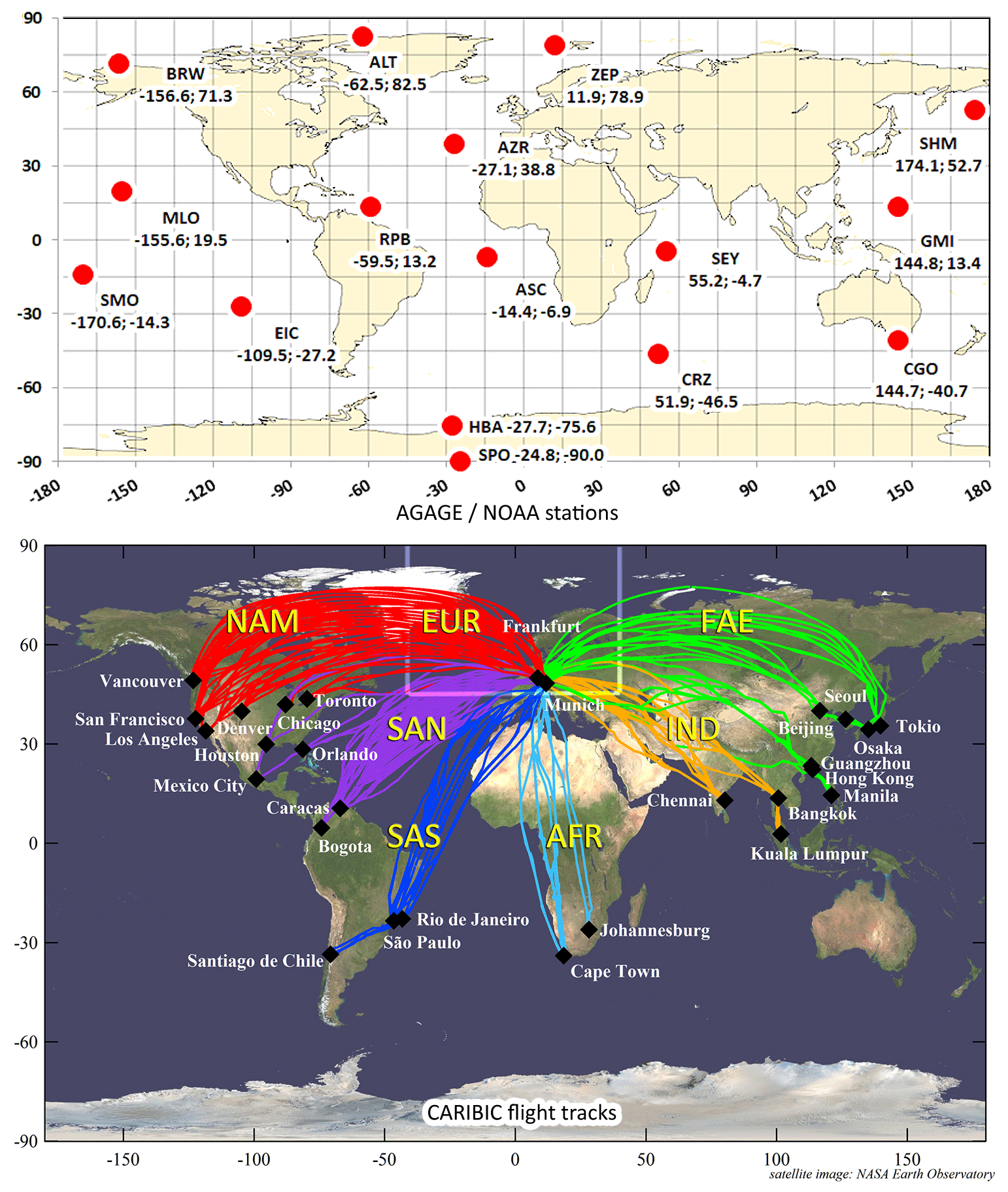
Figure 2 (a) Map of NOAA sampling locations for greenhouse gases used for reference in this study (see Table 1 for names and coordinates). (b) CARIBIC flights and destinations (1996–2014).

3.1 NOAA and AGAGE station network

The NOAA Global Greenhouse Gas Reference Network measures the atmospheric distribution and trends of the three main long-term drivers of climate change including methane (CH₄), the subject of this study. The Reference Network is part of NOAA's Earth System Research Laboratory in Boulder, Colorado (https://www.esrl.noaa.gov/gmd/ccgg/, last access: 29 April 2020).

The data are filtered with respect to synoptic-scale pollution events (Dlugokencky et al., 2018). We take advantage of 16 stations approximately equidistantly distributed over the globe (Fig. 2a) and remote from the major emission areas to ensure comparability with the model results which are not filtered. For the same reason, in the case of Cape Grim, Australia (41^∘ S, 145^∘ E), we refer to the unfiltered AGAGE records (Prinn et al., 2016). At all stations, monthly mean mixing ratios are compared to respective monthly averaged model samples.

3.2 CARIBIC flight observations

CARIBIC (Brenninkmeijer et al., 2007) is a passenger aircraft based atmospheric composition monitoring project that has become part of the In-Service Aircraft for a Global Observing System (IAGOS) infrastructure (http://www.iagos.org, last access: 29 April 2020). CARIBIC deploys an airfreight container equipped with about 1.5 t of instruments, connected to a multi-probe air inlet system. The container is installed monthly for four sequential measurement flights from and back to Frankfurt or Munich airport after which air samples, aerosol samples, and data are retrieved. The container houses instruments for measuring ozone, carbon monoxide, nitrogen oxides, water vapor, and many more trace gases as well as atmospheric aerosols. Air samples are collected at cruise altitude between about 10 and 12 km, and depending on latitude and season and actual synoptic meteorological conditions represent tropospheric or stratospheric air masses.

The spatiotemporal distribution of the CARIBIC methane sampling is quite different from that of the surface stations. Measurements were taken over relatively short time intervals and more than 96 % of the samples are from the NH. In contrast to the monthly average station data, the CARIBIC individual methane observations in the upper troposphere and lower stratosphere (UTLS) are based on air sampling over 20 min (i.e., ∼300 km) for CARIBIC-1 (1996–2002) and about 2 min (i.e., ∼30 km) for CARIBIC-2 (2002–2006), and appear to be much more variable compared to the stations. The sequence of sampling is irregular in time; i.e., the same destinations are reached through different flight routes (Fig. 2b), and take place during different times of the year. Thus, the associated statistics are not directly comparable to the station observations.

Overall, the ratio between sampled stratospheric and tropospheric air masses is about 0.5. These air samples are analyzed in the laboratories of the CARIBIC partner community. More than 40 gases are measured, including hydrocarbons, halocarbons, and greenhouse gases including CH₄. Methane mixing ratios in air samples were determined at the Max Planck Institute for Chemistry (MPIC). Sampling coordinates along flight tracks over regions such as Europe (EUR), North America (NAM), South America – north (SAN), South America – south (SAS), Africa (AFR), India (IND), and the Far East (FAE), and are color coded in Fig. 2b. These values, interpolated in time and space onto the model grid, are the subject of our evaluation.

The calibration is carried out using the NOAA methane World Meteorological Organization (WMO) scale (Dlugokencky et al., 2005). For further information about CARIBIC-based studies involving CH₄, we refer to Schuck et al. (2012), Baker et al. (2012), and Rauthe-Schöch et al. (2016). For the period 1997–2002, we use data from the first phase of CARIBIC (Brenninkmeijer et al., 1999). In this work, the CARIBIC data are based on monthly flight series (nominally four sequential long-distance flights).

The CARIBIC observatory provides an additional global constraint of CH₄ abundance and variability in the UTLS, not directly affected by emission sources at the surface, while being sensitive to the vertical exchange of air masses between the lower and upper troposphere.

4 The period 1997–2006

Using the a priori emission estimates, in the course of three subsequent 10-year simulations of the period 1997–2006, a 1997 initial CH₄ distribution was derived, representing a quasi-steady-state global CH₄ mass. A fully steady state was not possible due to the biomass burning a priori interannual variability, which adds interannual variability to the total methane of about 3.4 %. It must be stressed that each emission category experiences different OH concentration distributions, depending on the emissions patterns/regions. Therefore, each tagged CH₄ tracer has a different lifetime, which varies somewhat around the integral lifetime τ≅8.60 years. The individual steady-state lifetimes are quantified in Sect. 4.1.1 and listed in Table 1, column 5.

4.1 Emission scaling based on NOAA/AGAGE station observations

Based on the a priori emission assumptions (Table 1, column 3), the 2000–2006 average CH₄ mixing ratio over all AGAGE/NOAA stations of 1780 nmol mol⁻¹ is simulated within a RMSD of 0.40 %. With the applied initial distribution and emissions, the model reproduces both the 1997–1999 trend and the period without trend from 2000–2006. This suggests that the global CH₄ concentration in the period 2000–2006 represents the steady state after previously increasing emissions, probably until the early 1990s.

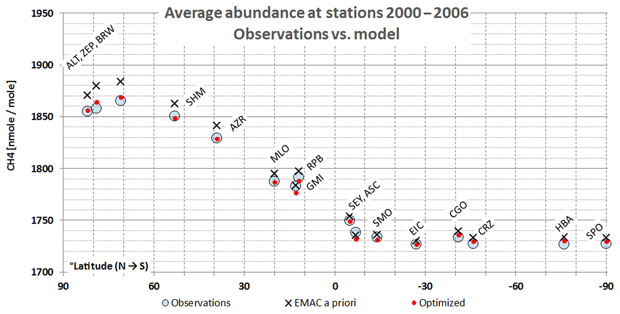
Figure 3 Optimization of calculated ground station CH₄ mixing ratios towards observations (blue circles): a priori simulations (black crosses) – a posteriori simulations (red dots).

Consistent with the observations, the simulated CH₄ mixing ratios are largest at Barrow (BRW) (71^∘ N) and decrease with latitude, reaching minimum values south of 40^∘ S at the Crozet Islands (CRZ) (46^∘ S), Halley Research Station (HBA) (76^∘ S), and SPO (90^∘ S). The abundance at AGAGE Cape Grim (CGO) (41^∘ S) is slightly enhanced and more scattered, being exposed to pollution events from the Australian continent, but also well reproduced by the model. The 2000–2006 (no-trend period) average observed mean mixing ratios for these stations range from 1865 to 1727 nmol mol⁻¹ and, using a priori emissions, are simulated within an average percentage RMSD of 0.67 %. Northern Hemisphere values, however, are overestimated, e.g., at BRW by 18.2 nmol mol⁻¹ (0.98 %), much more than the 5.7 nmol mol⁻¹ (0.33 %) at SPO (North Pole), and give rise to an overestimated interhemispheric difference (Fig. 3, black crosses vs. open blue circles), indicating mismatches in the emission assumptions. Although this imparity could also be caused by erroneous interhemispheric transport, previous analyses (Aghedo et al., 2010; Krol et al., 2018) show that the underlying ECHAM5 model realistically reproduces the interhemispheric transport time.

Taking advantage of the Solver (Sect. 2.4), we defined the goal as the minimum RMSD between the station measurements and respective model simulations composed of the tagged components multiplied with scaling factors, i.e., the parameters. Likely tolerance intervals are defined in a way that a posteriori mixing ratios are constrained by the 2000–2006 observations, which serve as objective criteria throughout this study. Emission amounts, rescaled with the obtained factors, are suitable to explain the observed abundances. The optimization effect on the emission categories is summarized in Table 1, column 4, and graphically displayed in Fig. S4. Hence, the net reduction of just 1.4 Tg yr⁻¹ (0.24 % of the total) underlines the general consistency of the a priori assumptions. While anthropogenic emissions typically influencing the Northern Hemisphere have been reduced in the a posteriori emissions (from 42 to 36, from 35 to 31, from 48 to 43, and from 68 to 65 for coal, oil, gas, and landfills, respectively), as well as those from ruminants (from 98 to 85 Tg yr⁻¹), other sources like wetlands (from 133 to 151 Tg yr⁻¹), rice paddies (from 60 to 63 Tg yr⁻¹), and minor predominantly Southern Hemisphere sources like biomass burning (from 20 to 22 Tg yr⁻¹), termites (from 19 to 22 Tg yr⁻¹), and biofuel combustion (from 15 to 17 Tg yr⁻¹) have been increased. The revised global CH₄ EMAC distribution has been composed of the sum of the tagged methane tracers proportional to the a posteriori emissions. The resulting station mixing ratios are marked by red dots in Fig. 3.

The a posteriori RMSD from the all-station average mole fraction improves from 0.67 % to 0.41 % with respect to the all-station 2000–2006 mean. The all station coefficient of determination R²=0.79 confirms the good agreement with observed variability (see scatter plots in Fig. 4 for individual stations: ALT, RPB, and SPO). The simulated 2000–2006 average interhemispheric difference of a priori 143.12 nmol mol⁻¹ was improved to 131.28 nmol mol⁻¹ by the optimization procedure and quite well matches the respective observation (130.82 nmol mol⁻¹). It appears that the ruminant animal emissions are scaled down due to a too-steep NH/SH gradient which hampers the optimization of the shape of the total distribution.

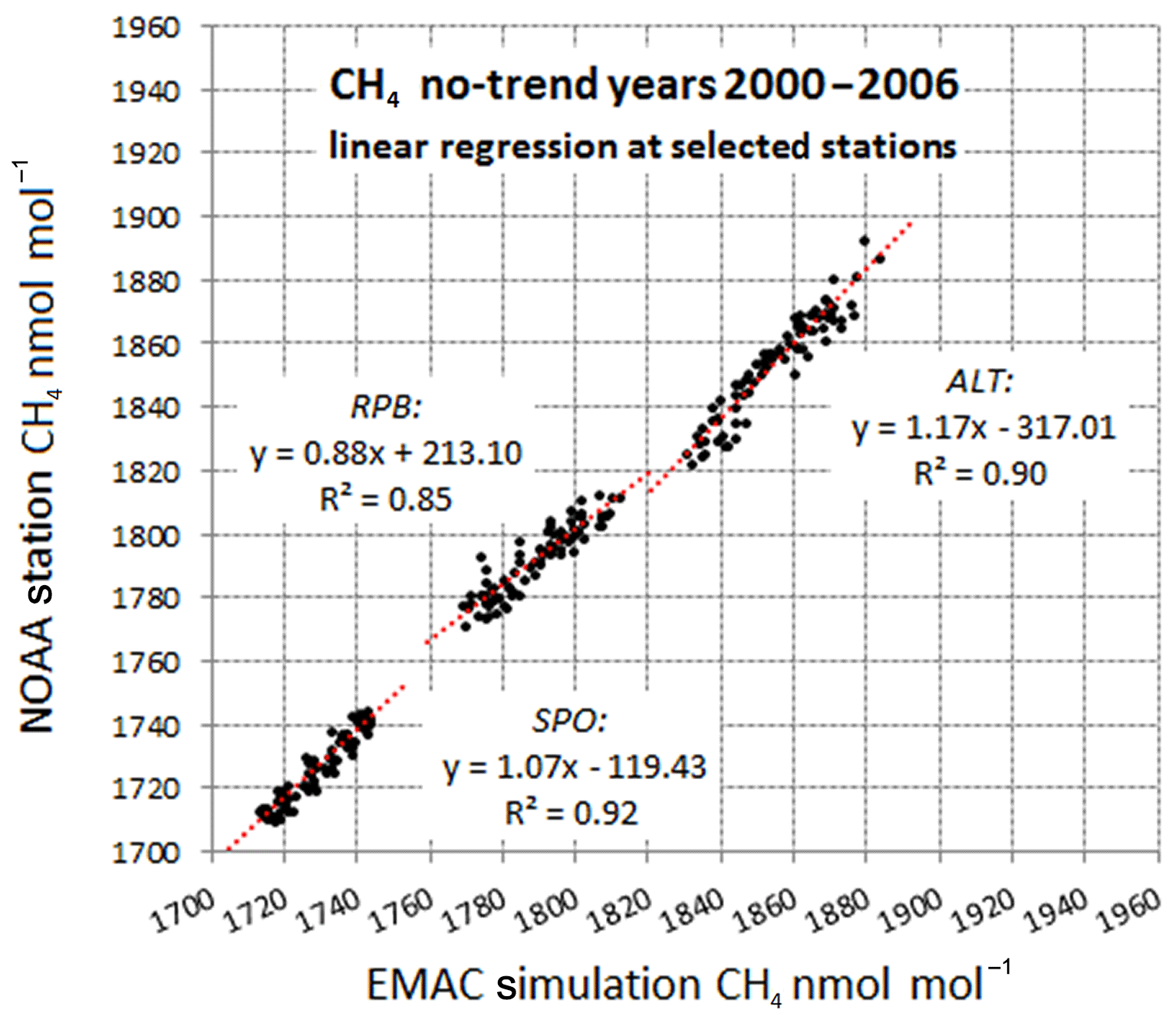
Figure 4 Regression analysis of EMAC calculations vs. observations of CH₄ at NOAA stations ALT, RPB, and SPO for no-trend years (2000–2006).

Figure 5 EMAC calculations (red) vs. NOAA and AGAGE observations (blue) of CH₄ from 1997 to 2006.

Figure 5 shows a posteriori simulation results based on the revised emissions together with the measurement at five representative observation sites.

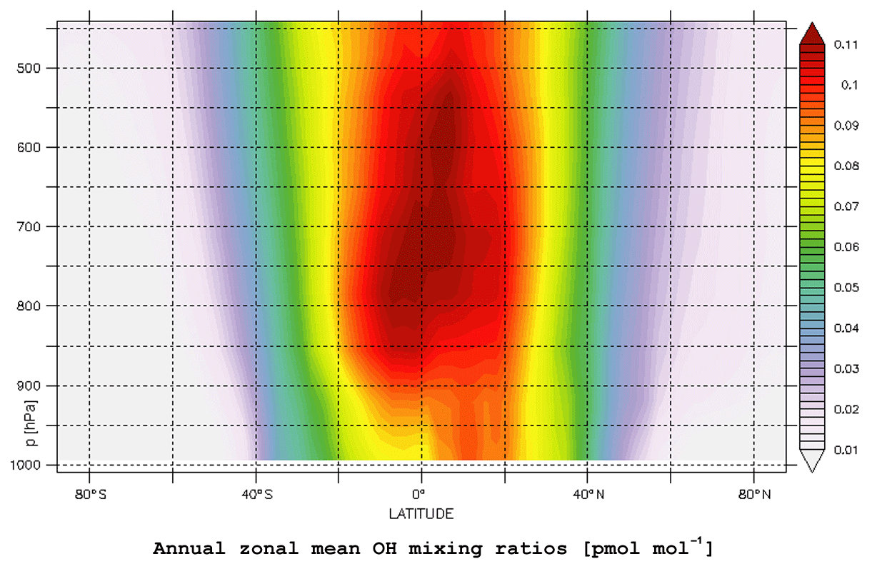
Figure 6 In the Northern Hemisphere lower troposphere, the OH mixing ratios are considerably higher than on the Southern Hemisphere.

The tagged tracers are proportional to the respective emission amounts but influenced by the distance from the source due to the oxidation by OH. Footprints at stations are the result of source and sink interactions (Fig. S5). For the same source strength, the atmospheric abundance is lower at a shorter distance between source and sink, and vice versa. This is quantified in terms of the “steady-state lifetime”, defined as the ratio between the global atmospheric trace mass (i.e., atmospheric burden) and the annual emission amount, which is, by definition of steady state, equal to the total annual sink. Over the period of relative stagnation (2000–2006) (Fig. 1), the shortest lifetimes (τ≅7.0 years) were found for Northern Hemisphere emissions experiencing the highest OH concentrations (Fig. 6). On the other hand, wetland methane (swamps) is exposed to lower OH concentration, producing a steady-state lifetime of τ=10.1 years (Table 1, column 7, and Fig. S6a). Biomass burning methane never establishes steady-state equilibrium because of the very irregular interannual intensity of the fire events (Fig. S6b). Considering that its contribution to the total emissions with ∼3.5 % is small, it is possible to quantify the total tropospheric CH₄ lifetime at τ≅8.60 years.

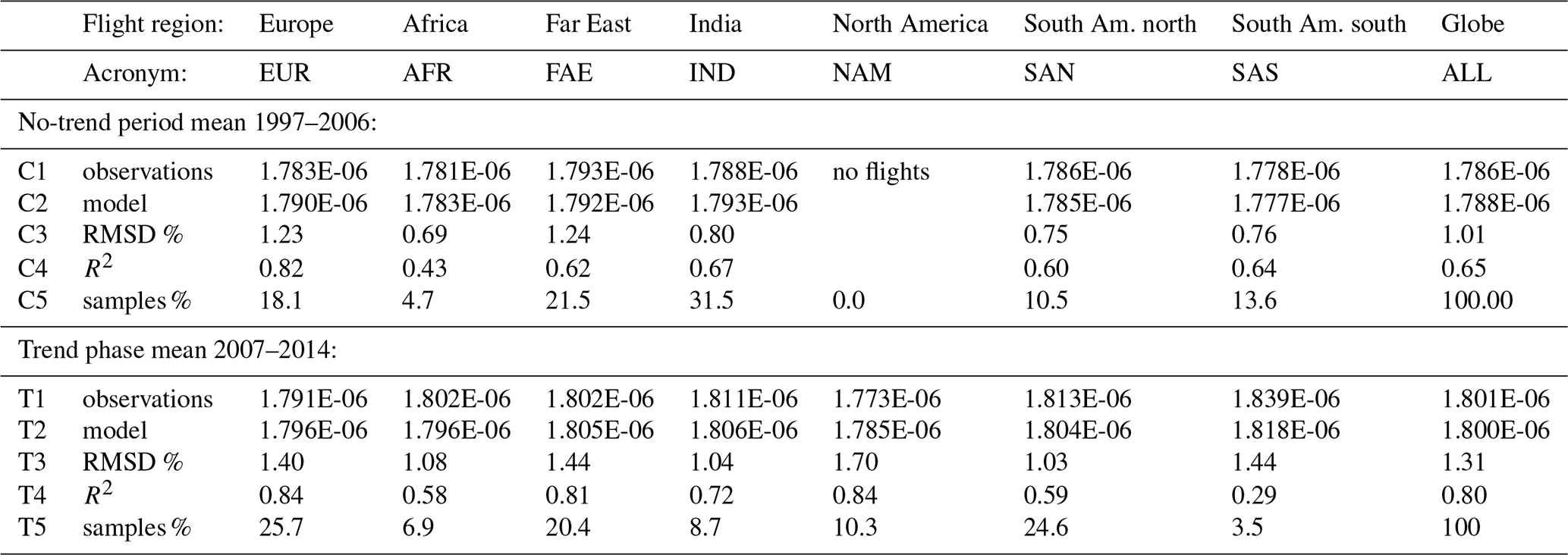
Table 2 Statistical evaluation of CARIBIC flight methane samples vs. EMAC model simulation results based on optimized emissions.

4.2 CARIBIC flights

Between 2000 and 2006, all CARIBIC observations average at 1786 nmol mol⁻¹. Corrected with respect to the a posteriori emission data based on the station analysis, the simulation average comes very close with 1788 nmol mol⁻¹. The whole period is well reproduced within an RMSD of 1.01 % and a coefficient of determination R²=0.65 (Table 2, rows C1–4). The scattered sampling positions cannot be accurately reproduced by the grid model (EMAC) because of its finite resolution. The observed CH₄ variability features short-duration events like the interception of methane plumes or, alternatively, relatively clean air episodes and especially also stratospheric air; however, the patterns are rather well reproduced (Fig. 7). The model appears to capture the variations well, even those which are subject to intercepting the upper troposphere and lowermost stratosphere at middle and high latitudes.

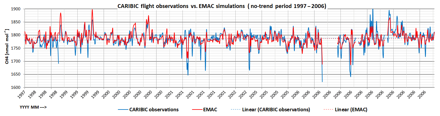
Figure 7 EMAC CH₄ calculations (red) and CARIBIC-1/2 observations (blue) from 1997 to 2006 – all flight samples.

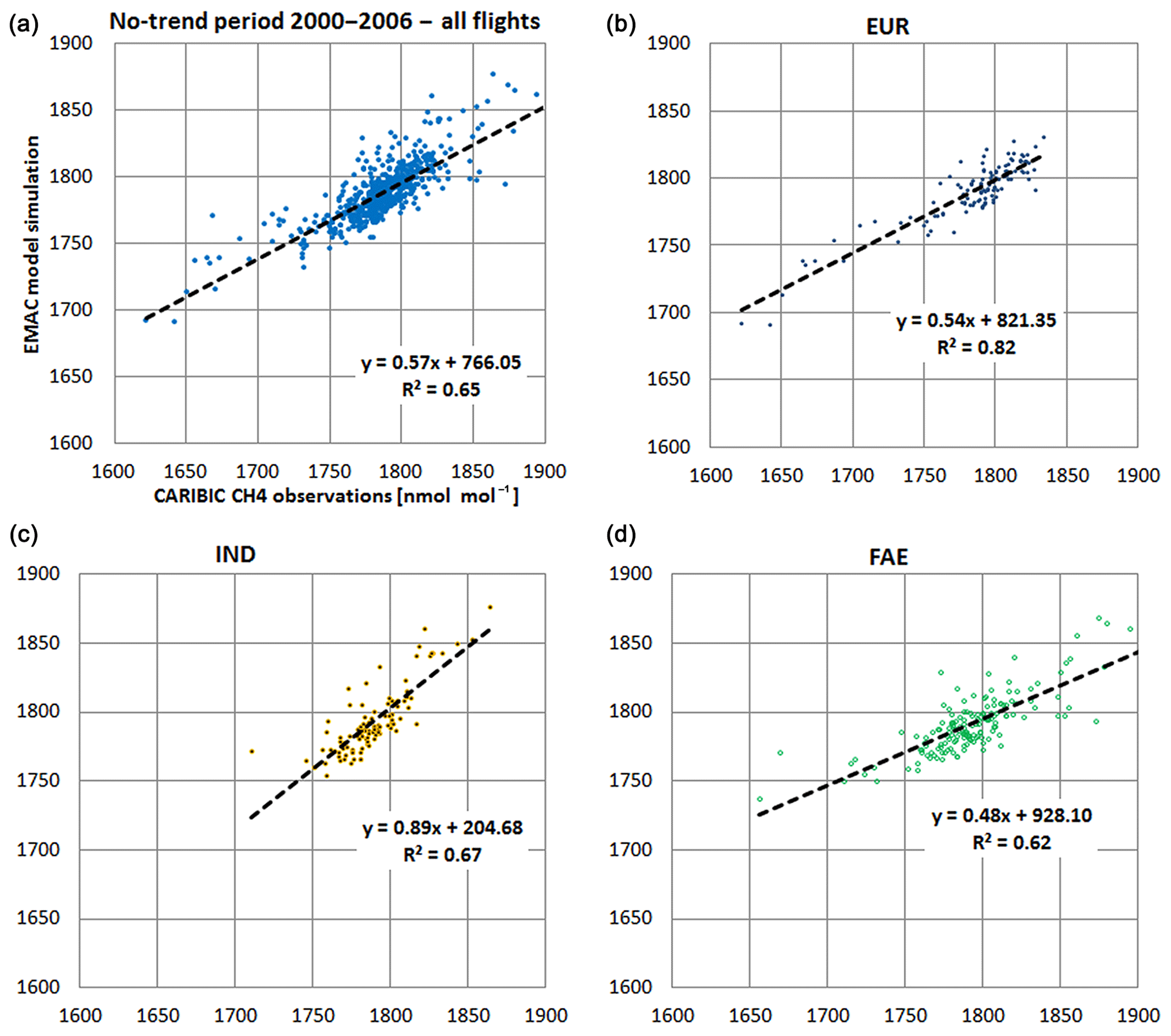
Figure 8 Correlation CARIBIC flight samples (x axis) vs. EMAC simulations (y axis) (nmol mol⁻¹) for all flights during the no-trend period (2000–2006) (a) and the main flight regions: India (IND), Europe (EUR), and the Far East (FAE).

The amplitudes of the model time series, however, are smaller due to the relatively coarse vertical grid spacing of the model, which represents the UTLS at a resolution of about 500 m – compared to ∼45 m near the surface. In contrast to background station measurements, for the CARIBIC time series, local maxima and minima are not only related to season but also to vertical gradient effects, especially due to the strong mixing ratio gradients across the tropopause. The scatter plot (Fig. 8a) shows a regression slope of 0.57, i.e., well below 1, which quantifies the evident underestimation of the calculated CH₄ variability in Fig. 7, suggesting that the vertical resolution of the model grid is not optimal to resolve the fine structure in the tropopause region. The slope is compensated by a corresponding offset up to 766 nmol mol⁻¹, explaining the good correspondence between simulations and observations in Fig. 7.

For further analysis, we grouped the data records in Fig. S7 by the six flight sampling regions defined in Sect. 3.2 (Fig. 2b): EUR, AFR, FAE, IND, SAN, and SAS (no NAM flights were performed before 2007). The best agreement between model results and observations in terms of RMSD is achieved over low-latitude regions such as IND with 0.80 % and SAN/SAS ≤0.75. Here, the effect of stratospheric air is least. At the same time, observations over continental areas in the midlatitude NH could nevertheless be simulated well within an RMSD range of 1.23 % (EUR) and 1.24 % (FAE). It appears that the variance of the CARIBIC measurements with R² > 0.60 is well reproduced everywhere and most accurately over EUR with R²=0.82 (Fig. 8). AFR is not discussed here because of the sparse number of samples of 4.7 % of all. The statistics are summarized in Table 2 (rows C1–5).

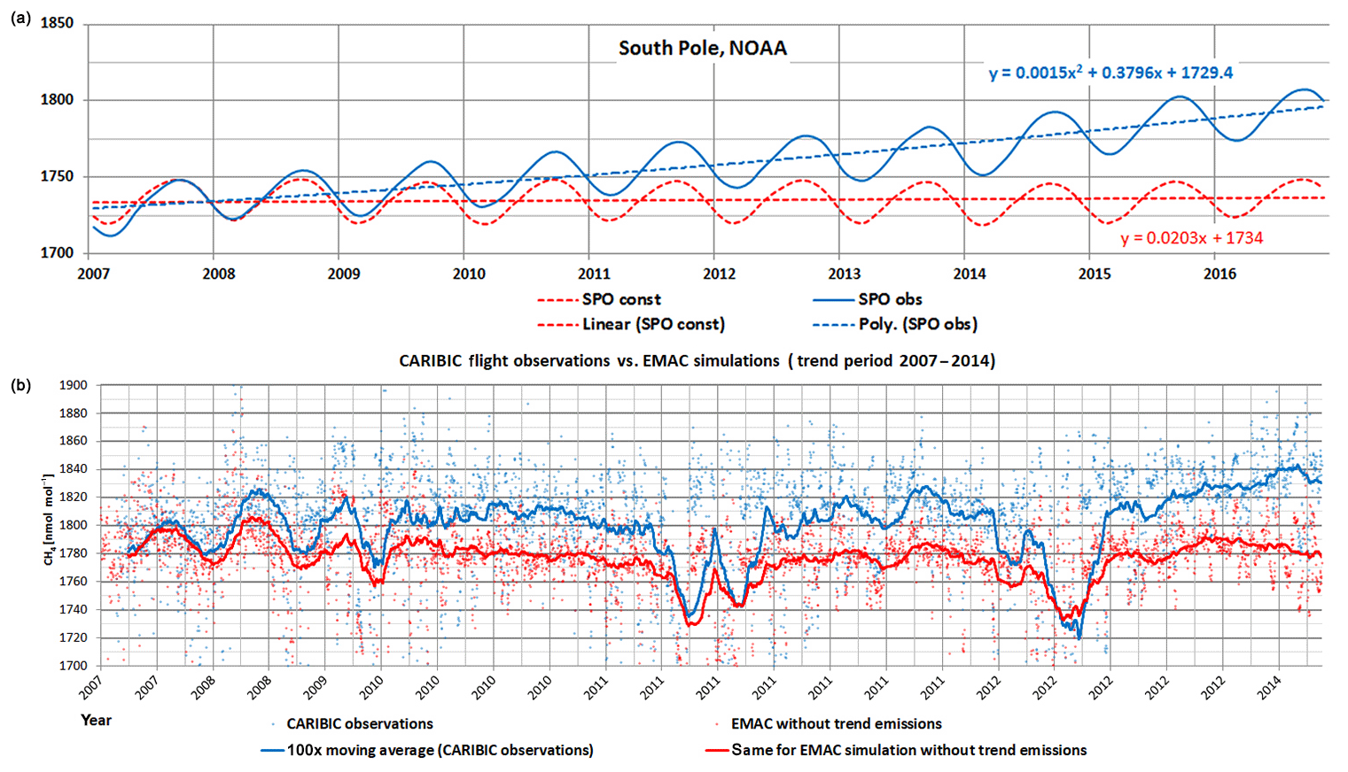
Figure 9 (a) NOAA observations at the South Pole (blue) from 2007 to 2016 compared to EMAC CH₄ calculations (red) under the 1997–2006 unchanged emission assumption; units are in nmol mol⁻¹. The observed trend is no longer linear and increasing after 2013 (following a second-order polynomial trend line, dashed blue). (b) CARIBIC flight observations (blue dots) compared to respective EMAC simulations without trend emissions (red dots); units are in nmol mol⁻¹. Superimposed lines represent respective 100× sliding means for better visibility.

5 Simulating the recent methane trend (2007–2013)

The measured methane increase, depicted by the blue lines in Fig. 9a for the NOAA background station data at SPO (90^∘ S) and in Fig. 9b for the CARIBIC flight records, cannot be reproduced by the model (red lines) based on interannually constant emissions. Between 2007 and 2013, the slope appears nearly linear (Fig. 1), and the discrepancy can be resolved by assuming an additional constant CH₄ source for this period. After 2013, the trend steepened and a further increment is required to explain the observations (Mikaloff-Fletcher and Schaefer, 2019). As mentioned above, we focus on the source strengths and neglect interannual changes in global OH. As mentioned in Sect. 2.2.1, four hypothetical source categories were added to our model simulation to reconcile the increasing post-2006 model vs. observation difference: enhanced emissions from tropical wetlands (scenario TRO), from agriculture including ruminant animals (ANI) and rice cultivation (RIC), and from shale gas drilling called fracking (SHA). For this period, the smallest RMSD (measurement vs. model) together with the coefficient of determination R² is also used as a criterion to evaluate the emission scenarios.

5.1 NOAA and AGAGE stations

The methane emissions scenarios defined above affect Northern Hemisphere as well as Southern Hemisphere observations. Under the influence of deep convection in the tropics and subsequent global transport, the characteristic seasonality of tropical emissions could influence the CH₄ time series worldwide. Shale-gas-associated emissions (SHA) from the Northern Hemisphere, however, need a relatively longer time period to influence CH₄ at Southern Hemisphere stations like the South Pole (SPO, 90^∘ S). The agricultural emissions cover parts of both hemispheres, and the North American SHA emissions are assumed to be seasonally independent. In our a priori assumption, each new emission sector has an emission increment of 20.5 Tg CH₄ yr⁻¹ starting in January 2007.

At first, the Solver was used to minimize the RMSD between model results and station observations for the case where each sector is the only responsible of the post-2006 trend. For this case, a posteriori emission amounts were calculated as 14.8, 15.9, 15.2, and 15.8 Tg yr⁻¹ for SHA, TRO, ANI, and RIC emissions, respectively.

Table 3 Statistical evaluation of rising-methane scenarios. RMSD from all-station observation mean in nmol mol⁻¹ CH₄.

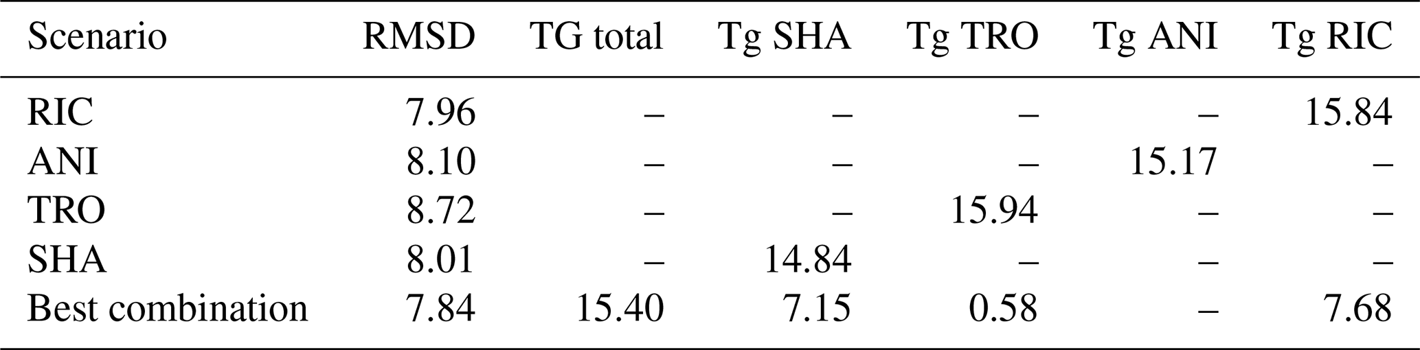
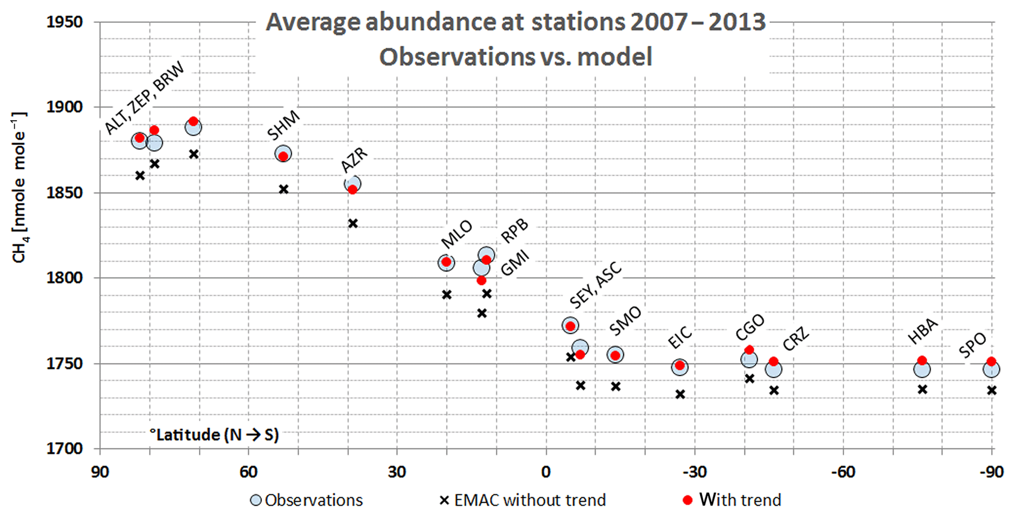
Figure 10 Calculated total CH₄ without (black crosses) and with optimized trend period emissions (red dots). By scaling RIC, SHA, and TRO emission fractions, the station observations (blue circles) are approximated with the smallest RMSD. After 2013, the trend accelerates and additional emission assumptions are necessary.

Secondly, we find an optimal combination of emissions of these four categories, with the constraint that the emissions must range between zero and the a priori upper limit of 20.5 Tg yr⁻¹. In this way, the most likely combination of sources excludes those from animals (ANI) in favor of 7.67 Tg yr⁻¹ CH₄ from SHA, 7.15 Tg yr⁻¹ from RIC, and a small TRO contribution of 0.58 Tg yr⁻¹ (i.e., 50 % RIC, 46 % SHA, and 4 % TRO emissions). The animal contribution is disregarded by the optimization procedure for the same reason as in Sect. 4.1.1., i.e., its overestimated NH/SH gradient. Table 3 presents a summary of all statistical metrics. Our results are in agreement with recent δ¹³C–CH₄ studies (Schaefer at al., 2016; Schwietzke et al., 2016), but it must be noted that the observed methane at the 16 NOAA stations considered here are at locations dominated by biogenic emissions and especially those from rice cultivation. Figure 10 depicts the CH₄ observations marked by open blue circles at all stations considered from north to south together with the respective no-trend simulations (black crosses) and the Solver-optimized increments (red dots). The respective scatter plots at selected NOAA stations (Fig. 11) indicate good correlation between the observed and calculated station monthly means. NOAA station records are displayed in Fig. 12, with optimized increments.

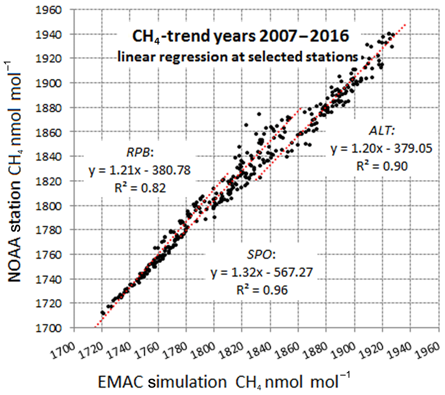
Figure 11 Regression analysis of EMAC calculations vs. observations of CH₄ at NOAA stations ALT, RPB, and SPO for the trend years 2007–2016.

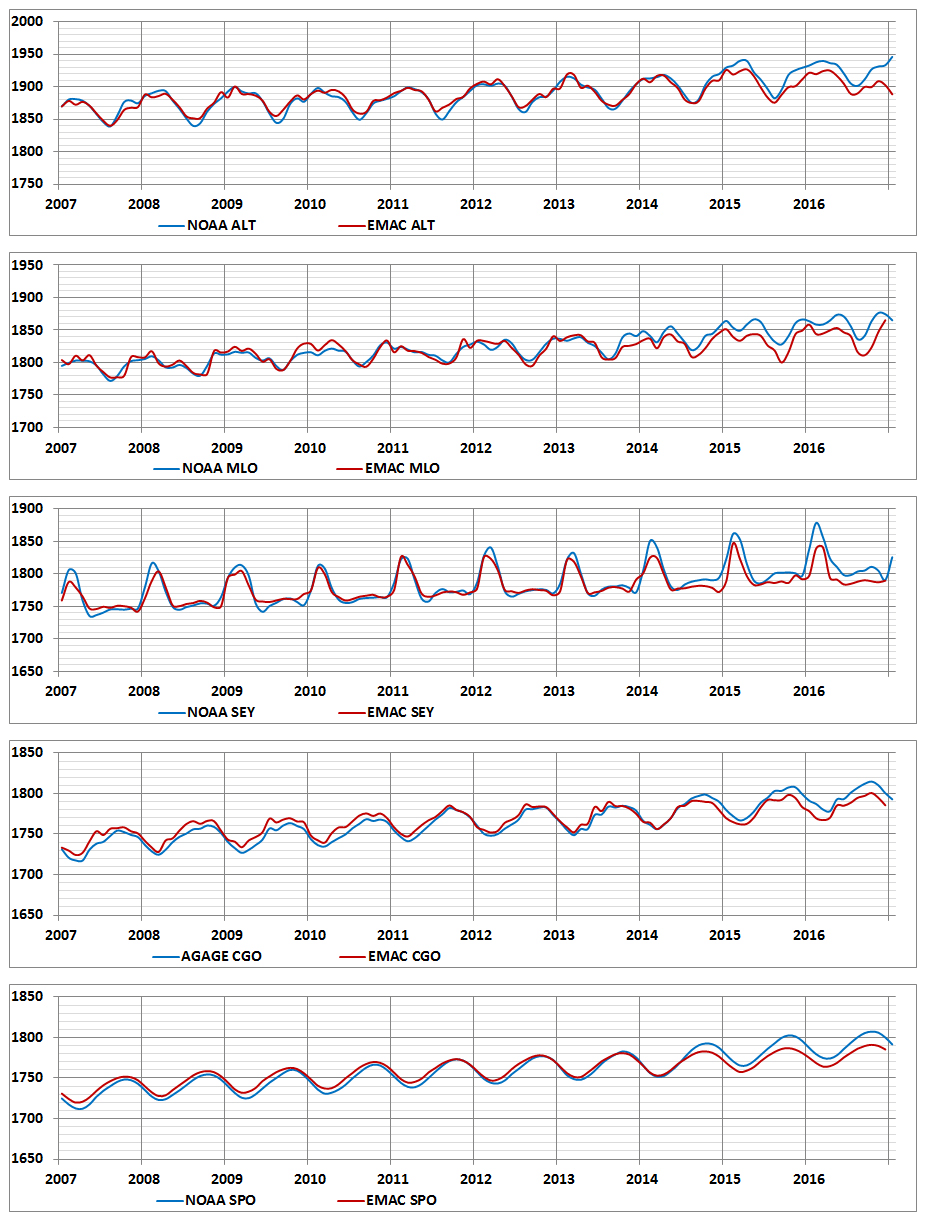
Figure 12 CH₄ development at NOAA and AGAGE stations (blue) vs. EMAC simulations (red) for the period 2007–2016; units of the mixing ratios are in nmol mol⁻¹. The trend emissions are optimized for the linear rising period (2007–2013).

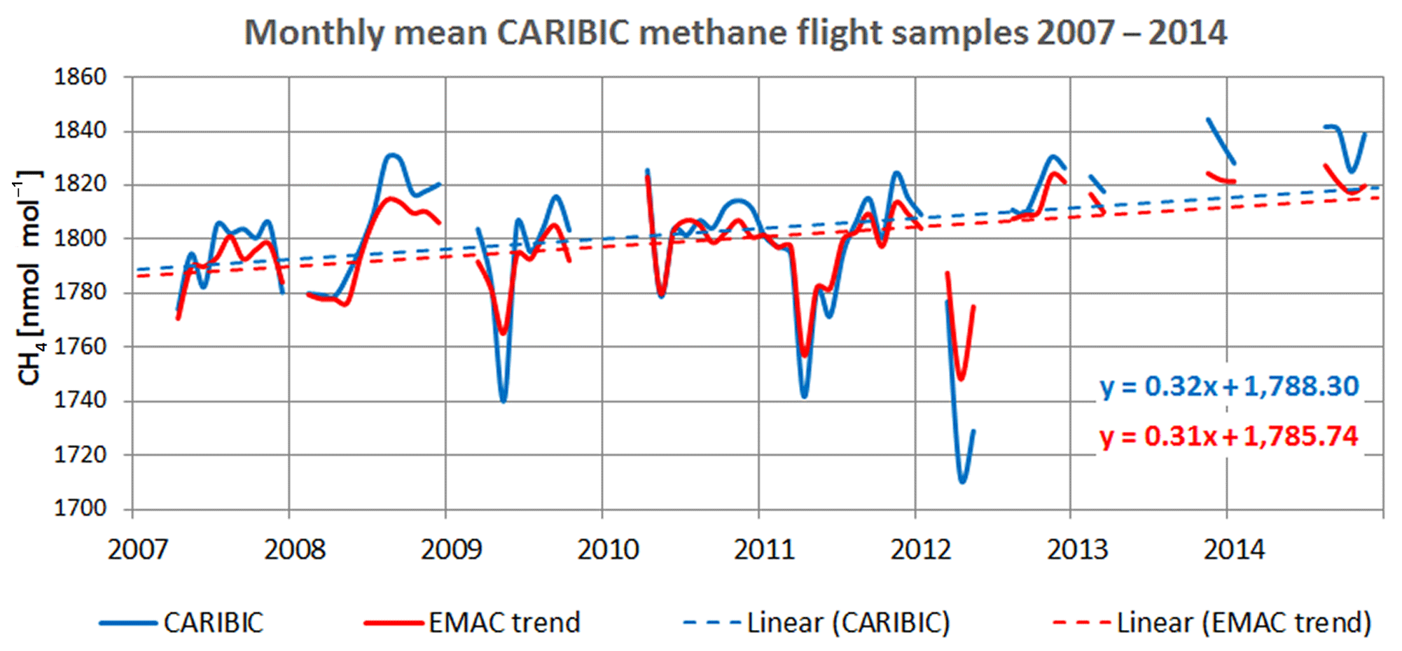
Figure 13 Monthly averaged EMAC-CH₄, including trend and CARIBIC-2 observations from 2007 to 2014 for all data obtained from CARIBIC whole air samples (WASs) in blue, and model results in red.

As a next evaluation, the longitudinal dependency of Northern Hemisphere anthropogenic fossil CH₄ emissions was investigated based on two options: one with the North American source redistributed to East Asia (FAE: 25–50^∘ N, 100–150^∘ E) and another to Europe (EUR: 45–60^∘ N, 0–26^∘ E). While no significant trend impact could be assigned to EUR, a hypothetical FAE contribution cannot be excluded. No evidence in favor of SHA or FAE can be identified at one of the stations in the Northern Hemisphere midlatitudes, probably related to the effects of synoptic-scale disturbances, the relatively intense latitudinal mixing and the > 8-year lifetime of CH₄.

Figure 14 Linear regression between CARIBIC-2 samples and EMAC calculations for all trend period flights (2007–2014) and for flight regions with more than 300 samples.

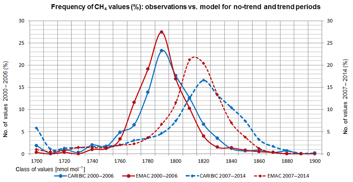
Figure 15 Frequency spectrum of CARIBIC-observed and EMAC-simulated CH₄ mixing ratios separately plotted for the years 2000–2006 and 2007–2014.

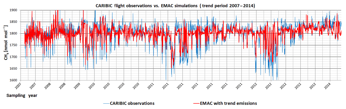
Figure 16 EMAC CH₄ calculations (red) and CARIBIC-2 observations (blue) from 2007 to 2014 – all flight samples.

5.2 CARIBIC flights

Using the a posteriori model results for the period 2006–2016 as described in Sect. 5.2.1, also the post-2006 CARIBIC-2 methane measurements appear to be realistically simulated by the EMAC model. In Fig. 13, monthly averaged CARIBIC measurements are plotted together with corresponding model results. The slopes of the linear trend in observations and model results indicate a very good model representation of the methane trend (0.32 vs. 0.31). The regression analysis with R²=0.8 over all flight samples (Fig. 14, upper left panel) shows a very good agreement between model results and aircraft observations. We re-emphasize that the model underestimates measured extremes, especially the downward excursions observed during Northern Hemisphere intercontinental flights in April and May 2009, 2011, and 2012 caused by tropopause folding events, which at the given model vertical grid spacing (∼500 m in the UTLS) cannot be satisfactorily resolved. This is confirmed by the frequency spectra (Fig. 15): median simulated values reveal higher amplitudes than measurements before and during the methane-trend period. The different widths of the frequency distributions σ=6.2 (EMAC) and 4.7 nmol mol⁻¹ (CARIBIC) for the period 2007–2014 and σ=7.4 and 6.3 nmol mol⁻¹, respectively, for the period 2000–2006 confirm the model favoring medium range values.

For a further comparison with the pre-2007 results, Fig. 16 depicts the whole series on a non-equidistant time axis. Focusing on individual flight sampling regions (Fig. S8), we restrict the statistical analyses (Fig. 14) to areas and periods with at least 300 samples. The highest coefficients of determination (R² > 0.8) are obtained for NAM, EUR, and FAE. For the other four regions reaching further south, such as SAN or IND, the influence of lower stratosphere sampling is stronger, leading to smaller linear slopes together with a comparably lower R² values of 0.59 and 0.72, respectively.

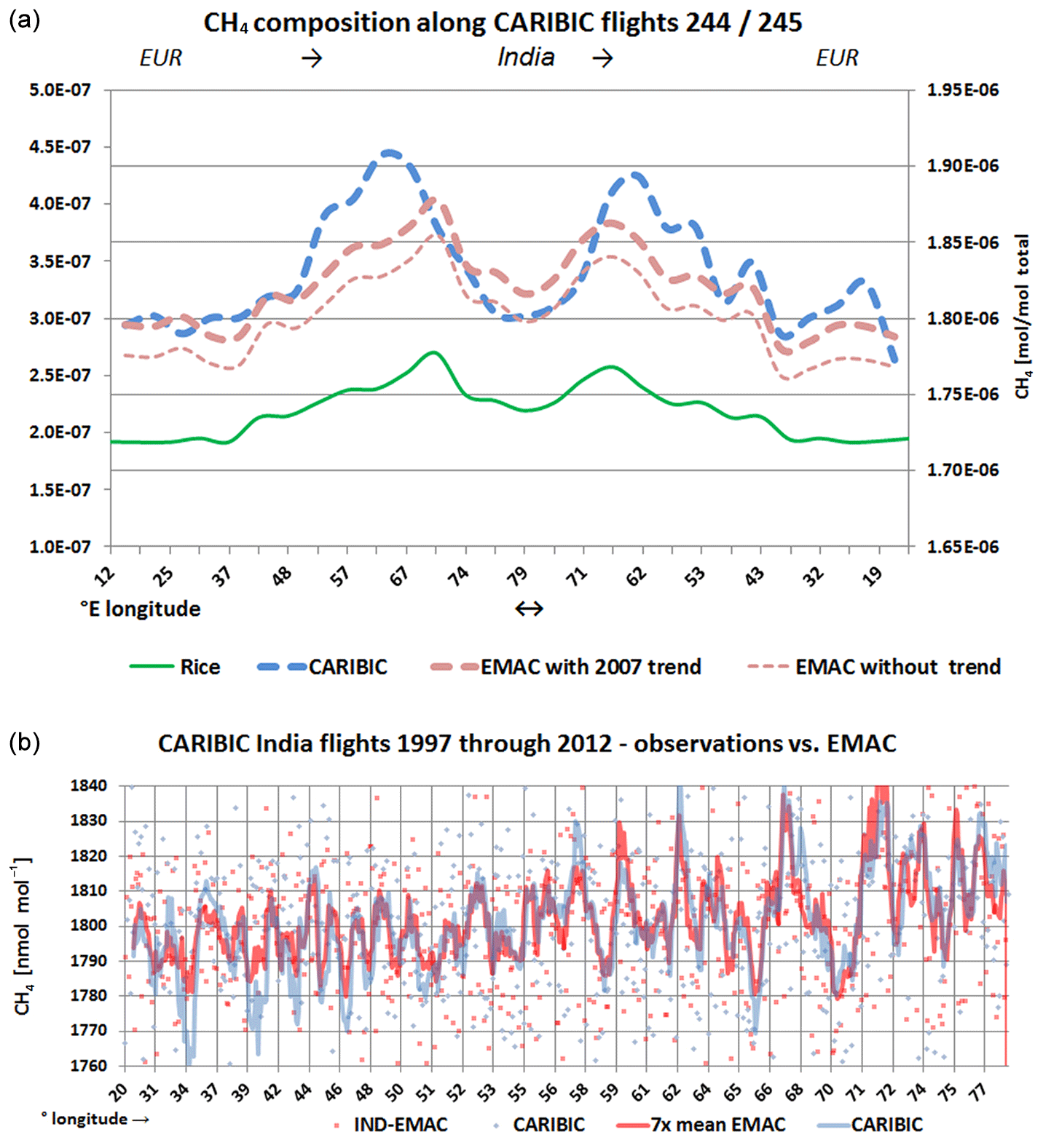
Figure 17 (a) CH₄ mixing ratios observed by CARIBIC (dashed blue, right axis) and calculated by EMAC (thick dashed red) and tagged rice-related CH₄ (green, left axis) – India flights (August 2008). The thin dashed red line marks the simulation without trend period increment for reference. (b) CH₄ mixing ratios (nmol mol⁻¹) observed by CARIBIC (blue) during all India flights (1997–2012) and corresponding EMAC simulations (red). The large scatter requires the sliding average of seven points (solid lines).

Selected CARIBIC flights

Individual flights show variations in CH₄ source composition in response to relatively small-scale influences. A striking demonstration of the varying influences of emissions in the model in regions crossed by the CARIBIC aircraft is provided by flights 244–245 on 13–14 August 2008, between Frankfurt in Germany and Chennai (formerly Madras) in India. In Fig. 17a (right ordinate), the total observed CH₄ mixing ratios along the flight track are plotted over the respective simulations (with and without trend increment). Typically, simulated peak values are underestimated and not correctly in phase with the observations. Figure 17b underlines this for the whole collection of India-bound CARIBIC flight samples in accordance with Fig. 15. The post-2006 increment in Fig. 17a ( thick red dashed vs. thin red dashed) is obvious but with 1.0 % on average still relatively small in 2008. The source-segregated rice paddy methane (green, left ordinate) dominates the pattern of the total CH₄ and the R²=0.65 implies that 0.65 % of the observed CH₄ variability along this specific flight track can be explained by rice paddy emissions. The largest mixing ratios in excess of 1850 nmol mol⁻¹ were recorded in the upper troposphere between 50 and 75^∘ E. Trajectory calculations as well as methane isotope and other chemical tracer analyses (Schuck et al., 2012; Baker et al., 2012) corroborate that these air masses carry emissions from southern and southeast Asia and can be explained by the trapping of air masses (Rauthe-Schöch et al., 2016) from southern Asia in the upper troposphere anticyclone (UTAC), a persistent phenomenon during the monsoon and centered over Pakistan and northern India (Garny and Randel, 2013; Tomsche et al., 2019). This is also qualitatively illustrated in Fig. S9. The methane released by rice paddies in southern Asia, trapped in the UTAC, obviously marks the local maximum in the total CH₄ distribution (Fig. S9b – different scales were used for better representation). The flight route crosses this pattern twice, from NW to SE and back. Further, relatively localized maxima in the Northern Hemisphere extratropics (red areas in Fig. S9a) are caused by anthropogenic sources such as coal mining and gas exploitation and from boreal bogs in summer.

Another demonstrative example for tagging results is presented in Fig. S10 which depicts CH₄ mixing ratios observed during the FAE flight 304 from Osaka, Japan, to Frankfurt (Main), Germany, in July 2010 together with respective tracers including four of the most relevant individual tagged source contributions. Calculations (thick dashed red, right axis) follow the phase of the measurements (blue dashed, right axis). The trend period increment (the difference between thick red and thin red lines) in 2010 with 1.5 % in average has significantly increased compared to 2008. The pattern is determined by animal, landfill, and natural gas source contributions. The coefficient of determination with respect to the observations is R²=0.77. The pronounced bog-methane profile (color coded in olive green) dominates the pattern but is not correctly in phase with CARIBIC in terms of R²=0.38. Rice fields east of 136^∘ E contribute relatively strongly. Additional systematic studies of the source segregated composition of all CARIBIC flights over the years 1997–2019, with special emphasis on the most recent trend development, will be subject of continued investigation.

6 Conclusion and outlook

We analyzed the atmospheric methane budget by means of EMAC model simulations and comparing results with data from NOAA and AGAGE surface stations and CARIBIC aircraft measurements. Source tagging is used to analyze the emission distribution and to optimize the respective amounts in relation to the observations. We found that, compared to a priori assumptions, a larger natural biogenic methane source with a concomitant reduction in NH fossil emissions is required to explain the measurements and especially the observed interhemispheric gradient.

Additional methane emission categories such as rice cultivation (RIC), ruminant animal (ANI), North American shale gas extraction (SHA), and tropical wetlands (TRO) have been investigated as potential causes of the resuming methane growth starting from 2007. In agreement with recent studies, we find that a methane increase of 15.4 Tg yr⁻¹ in 2007 and subsequent years, of which 50 % are from RIC (7.68 Tg yr⁻¹), 46 % from SHA (7.15 Tg yr⁻¹), and 4 % from TRO (0.58 Tg yr⁻¹), can optimally explain the trend up to 2013. After 2013, the trend steepened, and further observations beyond 2016 will be needed for a comprehensive assessment.

The model simulations described in this work rely to some degree on several assumptions, such as (i) no interannual variability of OH, (ii) constant geographical distribution for each source, (iii) no interannual variability of methane emissions with the exception of the causes of the post-2006 methane trend, and (iv) no interannual change in soil sink (only scaled by the methane mixing ratios in the boundary layer).

We optimized the sizes of individual emission categories, the most uncertain aspect of the methane budget, while the – comparably less critical – geographical distribution offers good criteria for optimization towards highly reliable measurement data.

Considering rapid zonal CH₄ transport relative to the CH₄ lifetime, the emissions presented here should rather be considered as representative of latitudinal sources than from specific locations, with the exception of those affected by large-scale convection, e.g., in monsoon areas, notably southern Asia. Nevertheless, the degree of freedom in the choice of sources is limited and our scenario realistically represents the north–south gradient of CH₄, which is a critical constraint.

As the CARIBIC flight measurements are ongoing, improved coverage in the Southern Hemisphere is expected in the near future, which will provide additional constraints for emission categories with similar latitudinal distribution patterns.

Appendix A

Table A1 Abbreviations.