Anthropogenic and volcanic point source SO₂ emissions derived from TROPOMI on board Sentinel-5 Precursor: first results

The paper introduces the first TROPOMI-based sulfur dioxide (SO₂) emissions estimates for point sources. A total of about 500 continuously emitting point sources releasing about 10 kt yr⁻¹ to more than 2000 kt yr⁻¹ of SO₂, previously identified from Ozone Monitoring Instrument (OMI) observations, were analyzed using TROPOMI (TROPOspheric Monitoring Instrument) measurements for 1 full year from April 2018 to March 2019. The annual emissions from these sources were estimated and compared to similar estimates from OMI and Ozone Mapping Profiling Suite (OMPS) measurements. Note that emissions from many of these 500 sources have declined significantly since 2005, making their quantification more challenging. We were able to identify 274 sources where annual emissions are significant and can be reliably estimated from TROPOMI. The standard deviations of TROPOMI vertical column density data, about 1 Dobson unit (DU, where 1 DU $=\mathrm{2.69}\times {\mathrm{10}}^{\mathrm{16}}$ molecules cm⁻²) over the tropics and 1.5 DU over high latitudes, are larger than those of OMI (0.6–1 DU) and OMPS (0.3–0.4 DU). Due to its very high spatial resolution, TROPOMI produces 12–20 times more observations over a certain area than OMI and 96 times more than OMPS. Despite higher uncertainties of individual TROPOMI observations, TROPOMI data averaged over a large area have roughly 2–3 times lower uncertainties compared to OMI and OMPS data. Similarly, TROPOMI annual emissions can be estimated with uncertainties that are 1.5–2 times lower than the uncertainties of annual emissions estimates from OMI. While there are area biases in TROPOMI data over some regions that have to be removed from emission calculations, the absolute magnitude of these are modest, typically within ±0.25 DU, which can be comparable with SO₂ values over large sources.

1 Introduction

Sulfur dioxide (SO₂) is a major air pollutant that contributes to acid rain and aerosol formation, adversely affects the environment and human health, and impacts climate. Current and accurate information about SO₂ emissions is therefore required in modern air quality and climate models (e.g. Liu et al., 2018). The majority of SO₂ emissions are related to anthropogenic processes (e.g. combustion of sulfur-containing fuels, oil refining processes, metal ore smelting operations), although natural processes such as volcanic eruptions and degassing also play an important role. Information about emissions from SO₂ sources is not always available or up to date, and a sizable fraction of emission sources is even missing from conventional emission inventories (McLinden et al., 2016), with satellite measurements only now being used to fill this gap. Liu et al. (2018) demonstrated that merging such satellite-based emissions estimates with a conventional bottom-up inventory improves the agreement between the model and surface observations.

In the early 1980s, satellite measurements of backscattered radiation by the Total Ozone Mapping Spectrometer (TOMS) provided the first global estimates of SO₂ from large volcanic eruptions (Krueger, 1983). The TOMS instrument was capable of measuring backscattered solar ultraviolet (BUV) radiance at just several wavelengths. A hyperspectral instrument from the next generation (a UV–visible imaging spectrometer), the Global Ozone Monitoring Experiment (GOME) on the Earth Research Satellite 2 (ERS-2), launched in 1995, was able to detect major anthropogenic sources (Eisinger and Burrows, 1998; Khokhar et al., 2008). The launch of the Ozone Monitoring Instrument (OMI) on board NASA's Earth Observing System “Aura” satellite (Levelt et al., 2006, 2018), with high spatial resolution of up to 13 km by 24 km at nadir but lower at the swath edges (de Graaf et al., 2016), started a new era in satellite air-quality monitoring. Data from OMI, as well as from SCanning Imaging Absorption spectroMeter for Atmospheric CHartographY (SCIAMACHY) on the ENVISAT, the Global Ozone Monitoring Experiment-2 (GOME-2) on MetOp-A and MetOp-B (Callies et al., 2000), and the Ozone Mapping and Profiler Suite (OMPS) on board the NASA–NOAA Suomi National Polar-orbiting Partnership (Suomi NPP), were used to track SO₂ changes on the global and regional scales and estimate area and point source emissions (Carn et al., 2004, 2007; Fioletov et al., 2013; de Foy et al., 2009; Koukouli et al., 2016a, b; Krotkov et al., 2016; Lee et al., 2009; Li et al., 2017b; McLinden et al., 2012, 2014; Rix et al., 2012; Nowlan et al., 2011; Thomas et al., 2005; Zhang et al., 2017). Moreover, OMI measurements were used to evaluate the efficacy of cleantech solutions in reducing SO₂ emissions from industrial sources (Fioletov et al., 2013, 2016, 2017; Ialongo et al., 2018; Song and Yang, 2014).

There are two major types of UV–visible SO₂ retrieval algorithms for nadir viewing instruments. The traditional differential optical absorption spectroscopy (DOAS) scheme is based on the approach where absorption cross sections of relevant atmospheric gases are adjusted by a non-linear least squares fit procedure to the log ratio of a measured earthshine spectrum and a reference spectrum in a given wavelength interval (Theys et al., 2015). The DOAS algorithm requires information about the absorption spectra of all trace gases, non-elastic rotational Raman scattering (Ring effect), and instrument characteristics. The uncertainties of the DOAS algorithm arise from the inaccurate modelling of the various physical processes in solar light absorption and scattering (e.g. Ring effect, surface properties), as well as artifacts in the radiance measurements (e.g. stray light, wavelength shift). An alternative approach is used in the principal component analysis (PCA) algorithm. Instead of attempting to model all various factors other than SO₂, the PCA algorithm replaces them with characteristic features derived directly from the measurements over locations where no SO₂ is expected (Li et al., 2013, 2017b, 2019a, b). When applied to OMI measurements, both DOAS and PCA algorithms produce similar results; however, the PCA-algorithm-based data show reduced data scattering and smaller biases compared to the DOAS-algorithm-based data (Fioletov et al., 2016).

The launch of the TROPOspheric Monitoring Instrument (TROPOMI) on board the Copernicus Sentinel-5 Precursor in October 2017 made it possible to monitor atmospheric pollutants with an unprecedented spatial resolution, 3.5 km by 7 km (Veefkind et al., 2012), which is at least 12 times better than the resolution of OMI. Since 6 August 2019, the spatial resolution has been further reduced in the flight direction; the TROPOMI ground pixel size is now 3.5 km by 5.5 km. It has already been demonstrated that TROPOMI can successfully monitor trace gases such as ozone (Garane et al., 2019), NO₂ (Griffin et al., 2019), HCHO (De Smedt et al., 2018), CO (Borsdorff et al., 2019), CH₄ (Hu et al., 2018), and even BrO (Seo et al., 2019), as well as cloud properties (Loyola et al., 2018). The operational TROPOMI SO₂ retrieval algorithm utilizes the DOAS approach (Theys et al., 2017), and early observations demonstrated the benefits of high spatial resolution for monitoring volcanic plumes (Hedelt et al., 2019; Theys et al., 2019; Queißer et al., 2019). However, these first studies were focussed on relatively high volcanic SO₂ levels. In this study, we perform an analysis of TROPOMI SO₂ observations that include smaller anthropogenic and volcanic degassing sources. We applied a previously developed technique (Fioletov et al., 2015) to estimate SO₂ emissions from TROPOMI observations. About 500 SO₂ sources, previously identified using OMI 2005–2015 data (Fioletov et al., 2016), were examined, and their emissions were estimated using TROPOMI data and then compared to emissions estimates from OMI and OMPS.

2 Data sets

2.1 Satellite SO₂ vertical column density data

The TROPOMI instrument on board the Sentinel-5 Precursor (S5P) satellite was launched on 13 October 2017. TROPOMI has the smallest spatial footprint, 3.5 km by 7 km (3.5 km by 5.5 km after August 2019), among the instruments of its class (Veefkind et al., 2012). TROPOMI measures spectra of backscattered solar light at 450 cross-track positions (or pixels) and provides daily global coverage. TROPOMI SO₂ Level 2 (/PRODUCT/sulfurdioxide_total_vertical_column) data, processed with the S5P operational processing system UPAS version 01.01.05 (Theys et al., 2017), were used in this study. In the first step of the algorithm, SO₂ slant column densities (SCDs), representing the effective optical-path integral of SO₂ concentration, were retrieved using the DOAS method. An additional background correction was applied to remove possible biases in SCDs after the spectral retrieval step. The spectral fitting was done using the 312–326 nm window, although two other spectral windows (325–335 nm and 360–390 nm) were used for retrievals in cases of very high volcanic SO₂. The final product, the SO₂ vertical column densities (VCDs), was calculated from SCDs using conversion factors (air mass factors). VCDs represent the number of SO₂ molecules (or total mass) in an atmospheric column per unit area. VCDs are commonly reported in Dobson units (DU) where 1 DU $=\mathrm{2.69}\times {\mathrm{10}}^{\mathrm{16}}$ molecules cm⁻². The standard TROPOMI SO₂ data product additionally includes VCDs calculated for three volcanic scenarios: when a 1 km-thick plum is located at ground level, at 7 km, and at 15 km. In this study we focussed on anthropogenic and degassing volcanic emissions and used only data corresponding to ground-level plumes.

OMI, a Dutch–Finnish, UV–visible, wide-field-of-view, nadir-viewing spectrometer on board NASA's Aura satellite was launched on 15 July 2004 (Schoeberl et al., 2006). Originally, it was able to provide daily global coverage with a resolution of up to 13 km by 24 km at nadir (de Graaf et al., 2016; Levelt et al., 2006), but now about half of its pixels are affected by a field-of-view blockage and stray light (the so-called “row anomaly”), and SO₂ cannot be retrieved successfully from those pixels. The OMI detector has 60 cross-track positions. In our previous studies (Fioletov et al., 2016; McLinden et al., 2016), we excluded data from the first 10 and last 10 cross-track positions from the analysis to limit the across-track pixel width from 24 to about 40 km. However, due to row anomaly, this currently limits the number of available pixels to 15–20. We found that excluding only the first and the last five cross-track positions does not change the emissions estimates noticeably but reduces their uncertainties, so only the first and last five pixels were excluded from the current analysis. NASA's operational planetary boundary layer (PBL) SO₂ Level 2 data product was used in this study (OMSO2; Li et al., 2019a). This data product is produced with the principal component analysis (PCA) algorithm (Li et al., 2013, 2017). The 310.5–340 nm spectral window was used for SO₂ retrievals. Detailed information on the OMI PCA SO₂ data sets and their characteristics are available elsewhere (Krotkov et al., 2016; McLinden et al., 2015). It should be noted that the OMI DOAS algorithm-based data product is also available (Theys et al., 2015). While the results of the two algorithms are somewhat different, particularly in large-scale biases, emissions estimates from the two algorithms demonstrate very similar results (Fioletov et al., 2016).

The OMPS Nadir Mapper on board the Suomi National Polar-orbiting Partnership (Suomi NPP) satellite operated by NASA and NOAA was launched in October 2011. The standard NASA OMPS SO₂ data product (NMSO2-PCA-L2) is based on the same PCA algorithm as the NASA OMI data product (Li et al., 2019b; Zhang et al., 2017). OMPS has a lower spatial resolution than OMI, 50 km by 50 km, but better signal-to-noise characteristics. OMPS SO₂ VCD data are retrieved for 35 cross-track positions. Similar to OMI data analysis, large OMPS pixels at the edges of the swath (rows < 2 or > 33) were excluded. Both OMI and OMPS SO₂ data are retrieved with the same PCA algorithm, and emissions estimates for the two satellite instruments are similar, although OMPS tends to miss or underestimate emissions from small sources (Zhang et al., 2017).

Suomi NPP and S5P are on the same orbit 3.5 min apart and cross the Equator at about 13:30 local time. Aura is on a similar polar orbit and crosses the Equator at about 13:45 local time. Therefore, we can assume that there is no difference in the measurements of the three satellite instruments related to diurnal variations of SO₂. The TROPOMI operational SO₂ data record starts in April 2018. In order to have 1 full year of data, we analyzed TROPOMI, OMI, and OMPS data for the period from April 2018 to March 2019.

For emission estimates, we examined SO₂ values within a 300 km radius from each emission source listed in the SO₂ point source catalogue (Fioletov et al., 2016). There are about 500 sources in the catalogue; however, many sources emitting SO₂ in the first years of OMI operation were below the OMI sensitivity level in 2018, either closed or now producing substantially reduced emissions due to scrubber installation. The most recent version of the SO₂ emissions catalogue is available from NASA's public archive (Fioletov et al., 2019) and at https://so2.gsfc.nasa.gov/measures.html (last access: 8 May 2020).

2.2 Air mass factors and data filtering

Data filtering was applied to OMI, OMPS, and TROPOMI SO₂ data before the analysis. The current retrieval algorithms are optimized for low (0.05) surface albedo; therefore, pixels that correspond to snow-covered high-albedo surfaces were excluded from the analysis. Measurements taken at high solar zenith angles (more than 70^∘) were also excluded. Only clear-sky data, defined as having a cloud radiance fraction (across each pixel) of less than 20 %, were used. Negative SO₂ values that were less than −3 DU were also excluded. Values lower than the −3 DU threshold produced negative emission values in some rare cases, while higher values affected the emissions estimates themselves. To eliminate cases of transient volcanic SO₂, days with high volcanic SO₂ values were excluded from the analysis. If the highest 10 % of SO₂ values near the analyzed site were above a certain limit on a particular day, all data from the entire day were excluded. The limit depended on the emission strength and varied from 6 DU for sources emitting less than 100 kt yr⁻¹ to 15 DU for sources emitting > 1000 kt yr⁻¹ (see Fioletov et al., 2016, for details).

Information on air mass factors (AMFs) is required to convert TROPOMI SCDs to VCDs. AMFs depend on SO₂ vertical profile shape, solar zenith angle, observation geometry, total ozone absorption, clouds, and surface reflectivity. In the operational TROPOMI data set, TM5 model calculations were used to obtain a priori SO₂ vertical profiles to calculate AMF for each TROPOMI pixel. The model estimates rely on “bottom-up” emission inventories derived from economic activity data and SO₂ emissions factors for known sources, so that in the case of a missing source in the inventory, the model SO₂ profile shape would be representative of clean background areas, causing calculated AMFs to be biased high and VCDs underestimated over that source.

The PCA algorithm uses spectrally dependent SO₂ Jacobians instead of AMFs. To make it consistent to the previous operational OMI band residual difference (BRD) algorithm, the present PCA algorithm assumes the same fixed conditions that correspond to typical summertime conditions in the eastern USA, and PCA retrievals can therefore be interpreted as having an effective AMF of 0.36 as in the BRD algorithm (Krotkov et al., 2006). However, a constant AMF does not represent conditions such as high elevations or enhanced aerosol loading. As in our previous studies (Fioletov et al., 2016; McLinden et al., 2016) a single site-specific AMF was calculated for each source (McLinden et al., 2014) and applied to both OMI/OMPS and TROPOMI estimated emissions.

As one of the main goals of this study is to compare TROPOMI SO₂ data and emissions estimates to those from OMI and OMPS, we used a constant AMF of 0.36 for illustration maps, while for the emissions estimates we converted TROPOMI SO₂ SCDs to VCDs using the same site-specific AMFs, thereby removing them as a potential source of variability. It should be also noted that the spectral fitting window used in the TROPOMI algorithm is different from the window in the PCA algorithm. However, we estimated that that effect is small (under 10 %) compared to other sources of uncertainties.

The SO₂ absorption cross section has a moderate temperature dependence, with absorption increasing for higher temperatures, and there is a difference in how this dependence was handled in TROPOMI and OMI/OMPS retrievals. In the TROPOMI spectral fit, an SO₂ cross section at 203 K was used, and then the retrieved VCDs were adjusted by applying an AMF correction factor using temperatures from the European Centre for Medium-Range Weather Forecast (ECMWF) operational model (Theys et al., 2017). The OMI/OMPS retrieval algorithm uses the SO₂ cross section at 293 K (Krotkov et al., 2006) without any adjustment. In this work, for consistency, we used TROPOMI SO₂ SCDs and converted them to VCDs using the same AMFs as we utilized for OMI and OMPS (without any temperature adjustment). However, that meant that the obtained TROPOMI VCDs corresponded to 203 K as the original TROPOMI SCDs were calculated for that temperature. To remove the systematic difference with OMI/OMPS data caused by the difference in cross-section temperature (203 K for TROPOMI vs. 293 K for OMI/OMPS), we increased the TROPOMI SO₂ VCDs by 22 % (see Theys et al., 2017, their Fig. 6, for justification).

2.3 Wind and snow data

The emission estimation algorithm requires wind data. As in several previous studies (Fioletov et al., 2015; McLinden et al., 2016), European Centre for Medium-Range Weather Forecasts (ECMWF) reanalysis data (Dee et al., 2011) (http://apps.ecmwf.int/datasets/, last access: 8 May 2020) were extracted for every satellite pixel. Wind profiles are available every 6 h on a 0.75^∘ horizontal grid and are interpolated in time and space to the location of each satellite pixel centre. The u and v (west–east and south–north, respectively) wind speed components were averaged for 1 km thick layers, and the winds for the layer that corresponds to the site altitude were used. The interactive multi-sensor snow and ice (IMS) mapping system data (Helfrich et al., 2007) were used to screen out pixels over snow-covered surfaces with high albedo.

3 TROPOMI SO₂

For brevity, from this point we refer to “SO₂ VCD” as simply “SO₂”. It can be expected of TROPOMI that a smaller pixel size would yield a lower signal-to-noise level. Figure 1 shows the standard deviation of SO₂ values at four sites, each located at different latitudes, as a function of the TROPOMI cross-track position. The selected sites have relatively low SO₂ emissions, so the standard deviations are determined by the instrumental noise and possible retrieval uncertainties. The standard deviations at the 20 cross-track positions at the edges of the swath are particularly high due to less across-track binning, which motivated our decision (in addition to a larger footprint) to exclude them from the analysis. There is also a clear increase in the noise from low to high latitudes with the noise standard deviations at a sub-polar site nearly double compared to tropical sites. Outside the tropical belt, there is also some seasonality in the standard deviation values, with higher values occurring in winter and lower values in summer (not shown) due to weaker signals at low Sun.

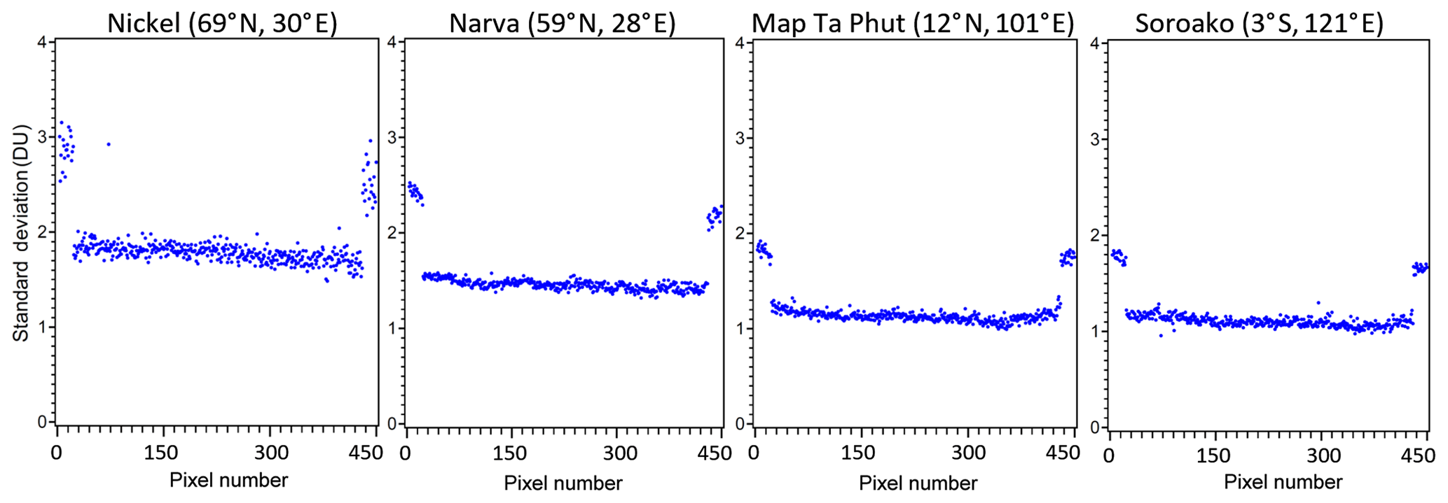
Figure 1 The SO₂ standard deviations as a function of the TROPOMI cross-track position (pixel number) at four sites illustrate a decline from high to low latitudes for the period from April 2018 to March 2019. The four sites selected represent sources with very low SO₂ emissions, and therefore the standard deviations represent the measurement uncertainties. The SO₂ values retrieved at the first and last 20 pixels have noticeably higher standard deviations and are excluded from the analysis.

The standard deviation of SO₂ retrievals for the three satellite instruments as a function of latitude is shown in Fig. 2 for the period from April 2018 to March 2019. The plot is based on satellite measurements over clean areas (150–300 km distance from the catalogue source locations) and represents background noise levels of SO₂. Large sources with annual SO₂ emissions above 1000 kt yr⁻¹ where the high standard deviations are likely to be influenced by the SO₂ variability itself were excluded from this analysis. Sources inside the South Atlantic Anomaly (SAA) region were also excluded. The standard deviations of TROPOMI data (about 1 DU over tropics and 1.5 DU over high latitudes) are larger than those of OMI (0.6–1 DU) and OMPS (0.3–0.4 DU) data. The standard deviations are particularly large (1.6–2.2 DU) for the first and the last 20 pixels in the TROPOMI 450-pixels-wide swath, which were excluded from further analysis.

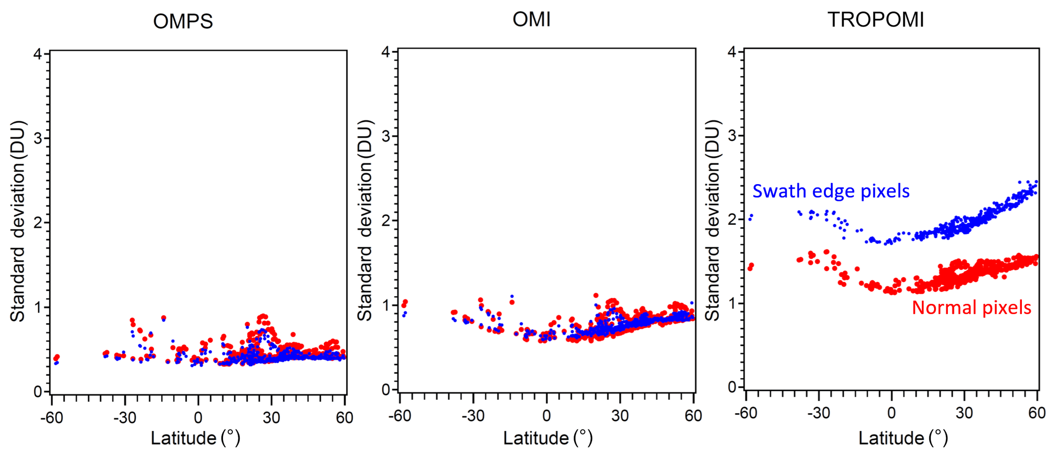
Figure 2 The OMPS, OMI, and TROPOMI SO₂ standard deviation vs. latitude for “normal” (red) and “swath edge” (blue) pixels. Swath edge pixels were defined as the first and the last 3, 5, and 20 pixels for OMPS, OMI, and TROPOMI, respectively. All other pixels were considered normal. The plot is based on satellite measurements centred between 150 and 300 km around the sources from the catalogue. The sources under the South Atlantic Anomaly (SAA) are excluded.

As Fig. 2 shows, the standard deviations (σ) for TROPOMI are roughly 1.5 time larger than OMI and 3 times larger than OMPS, since the TROPOMI footprint is smaller and each detector cell receives fewer photons than OMI and OMPS detector cells. However, the pixel size for TROPOMI is much smaller, and so the number of observations (n) over the same area for TROPOMI is 12 and 96 times that of OMI and OMPS, respectively. Considering these two factors, and assuming the standard error is proportional to $\mathit{\sigma }/\sqrt{n}$ (assuming that the errors of individual pixels are not correlated), then the uncertainty of a TROPOMI average will be roughly a factor of 2 smaller than OMI and a factor of 3 smaller than OMPS. In fact, due to the OMI row anomaly, the number of TROPOMI pixels over the same area is now a factor of 20 larger.

The global distribution of mean SO₂ from TROPOMI (smoothed using oversampling techniques or pixel averaging techniques with a 30 km radius; see e.g. Fioletov et al., 2011; Sun et al., 2018) is very similar to that from OMI and OMPS (Fig. 3). All three instruments clearly show elevated values over the Persian Gulf, China, Mexico, and India, as well as many anthropogenic “hotspots” such as Norilsk (Bauduin et al., 2014; Khokhar et al., 2008) and a cluster of power plants in South Africa, and large volcanic sources such as Kilauea, Hawai`i, and Ambrym, Vanuatu. All three satellite data sets shown in Fig. 3 do not demonstrate the large biases seen in the data of older versions of OMI, GOME-2, and SCIAMACHY (see Fioletov et al., 2013, their Fig. 1). Except for the hotspot-affected areas, SO₂ values from all three instruments are typically within the ±0.25 DU range. It is also interesting to note that the South Atlantic Anomaly (SAA), an area of increased flux of energetic solar wind particles that may intercept instruments in low-Earth orbits such as these, significantly increases the uncertainties of OMI and OMPS data (as well as data from GOME-2 and SCIAMACHY) but has little effect on TROPOMI data.

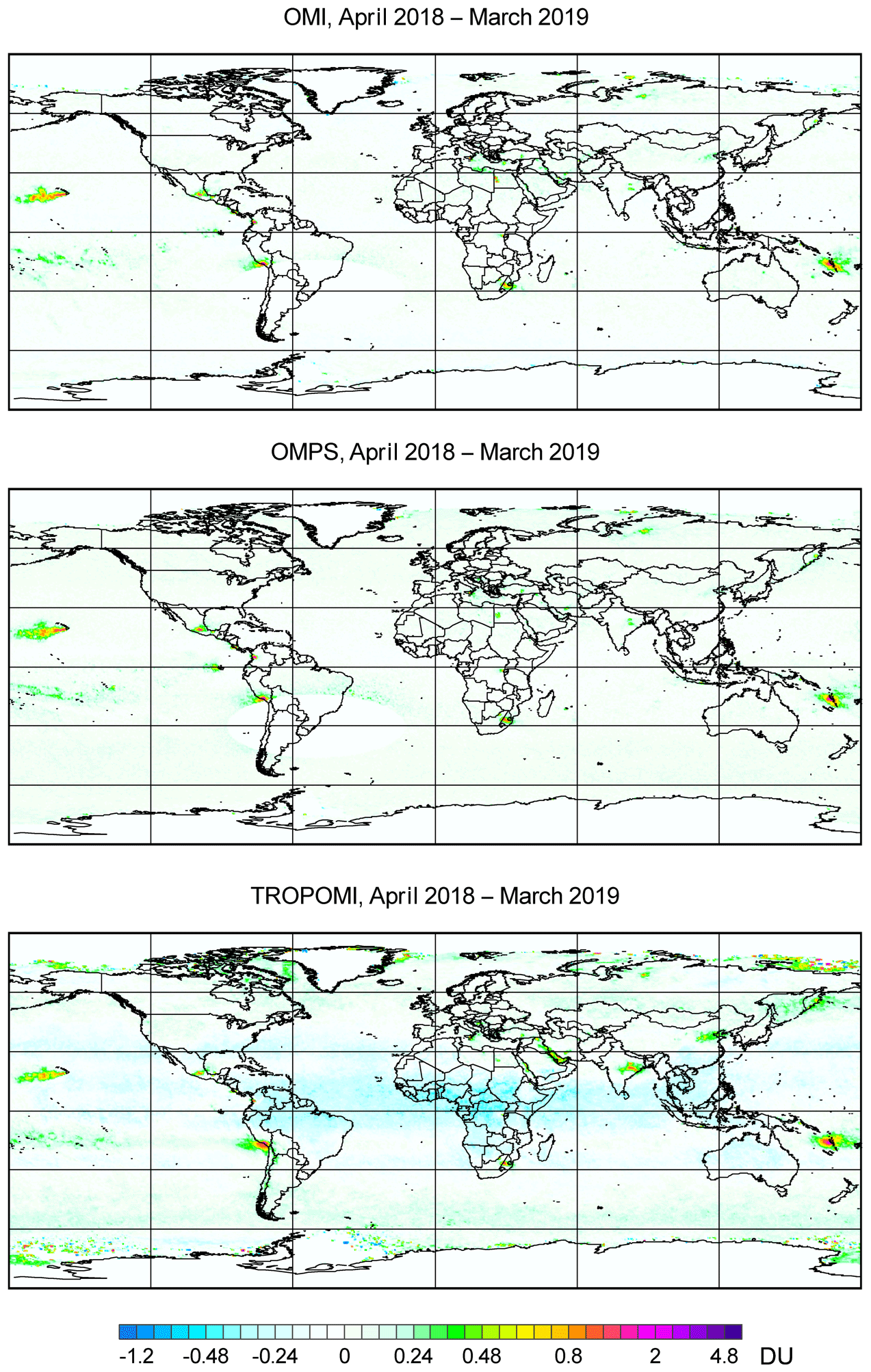
Figure 3 Mean SO₂ (DU) over the globe from TROPOMI, OMI, and OMPS for the period from April 2018 to March 2019. Data are smoothed by oversampling techniques with radius R=30 km. The area of the South Atlantic Anomaly (SAA) is left blank on the OMI and OMPS maps. The SAA greatly increases uncertainties of OMI and OMPS SO₂ data but has a much smaller effect on TROPOMI SO₂ data.

There are, however, still some differences in the absolute values between OMI, OMPS, and TROPOMI over some regions. Zoomed-in plots of mean SO₂ over four regions of elevated SO₂ values – northern China, India, Mexico, and Iran – are shown in Fig. 4. TROPOMI SO₂ means are, in general, higher than OMI and OMPS values over these regions, suggesting possible biases in TROPOMI data. The spatial scale of these biases (thousands of kilometres) is larger than the scale of elevated SO₂ values from a typical industrial source (100–200 km), so we will call them “large-scale biases”. Note that the biases are very small, only 0.1–0.2 DU; however, even such small biases could affect emissions estimates since the SO₂ enhancements from many sources are really tiny, a few tenths of a DU. These large-scale biases are common in satellite SO₂ retrievals. Their magnitude often depends on the retrieval algorithm, and the same satellite measurements (i.e. calibrated Level 1B data) processed with different SO₂ algorithms produce different biases. For example, GOME-2 data processed with the original operational algorithm (Valks and Loyola, 2009) had larger biases than the SO₂ data product based on the direct fitting method developed by the Harvard–Smithsonian Center for Astrophysics, Cambridge, Massachusetts (Nowlan et al., 2011; see Fig. 1 in Fioletov et al., 2013). The origin of such biases is not always known, although an imperfect removal of the very strong ozone absorption, which itself depends on stratospheric temperature and the shape of the ozone profile, could be one of the contributing factors.

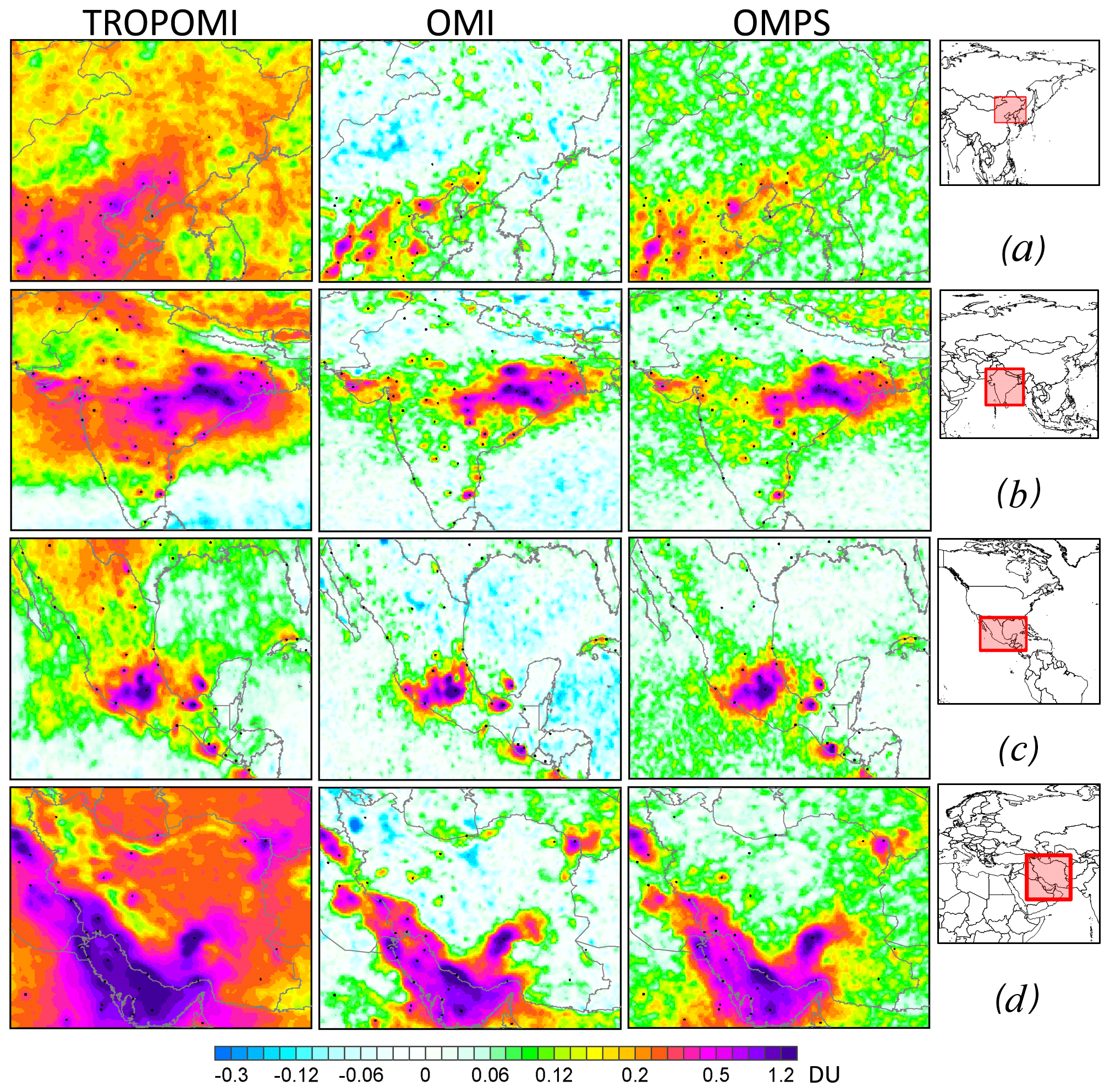
Figure 4 Mean SO₂ (DU) from TROPOMI, OMI, and OMPS over northern China (a), India (b), Mexico (c), and Iran (d) for the period from April 2018 to March 2019. Large-scale biases make it difficult to interpret TROPOMI SO₂ data and compare them to OMI and OMPS data directly. Data are smoothed by oversampling techniques with R=30 km. The black dots indicate the SO₂ sources. Note that the colour scale is different from the scale in Fig. 3.

OMI data processed with a DOAS algorithm (Theys et al., 2015), which is similar to the present TROPOMI algorithm, also had larger biases over some areas than those seen in the PCA-based data (Fioletov et al., 2016). However, as was also noted by Fioletov et al. (2016), both algorithms produce very similar results if the large-scale biases are removed, for example, by comparing up-wind and down-wind values around an SO₂ emissions source. In the case of large-scale biases in an area with multiple sources, the bias can be accounted for by introducing functions that change slowly with latitude and longitude as suggested by Fioletov et al. (2017). This multi-source algorithm accounts for the bias using Legendre polynomials of latitude and longitude, their products, and the emissions using functions that represent plumes from individual sources. As an example, Fig. 5 shows original data from TROPOMI, OMI, and OMPS over Europe and the same data with the local biases removed using sixth-degree polynomials (see Fioletov et al., 2017, for details). As Fig. 5 suggests, large-scale biases seen in the original TROPOMI data are removed by this statistical fitting procedure. Note that OMPS data also show some large-scale biases over that region. The maps with the large-scale biases removed look very similar for all three satellite data sources, and all the major SO₂ hotspots are clearly seen. Note that there is practically no bias in OMI data over southern Europe; hence, OMI data with and without biases removed appear very similar.

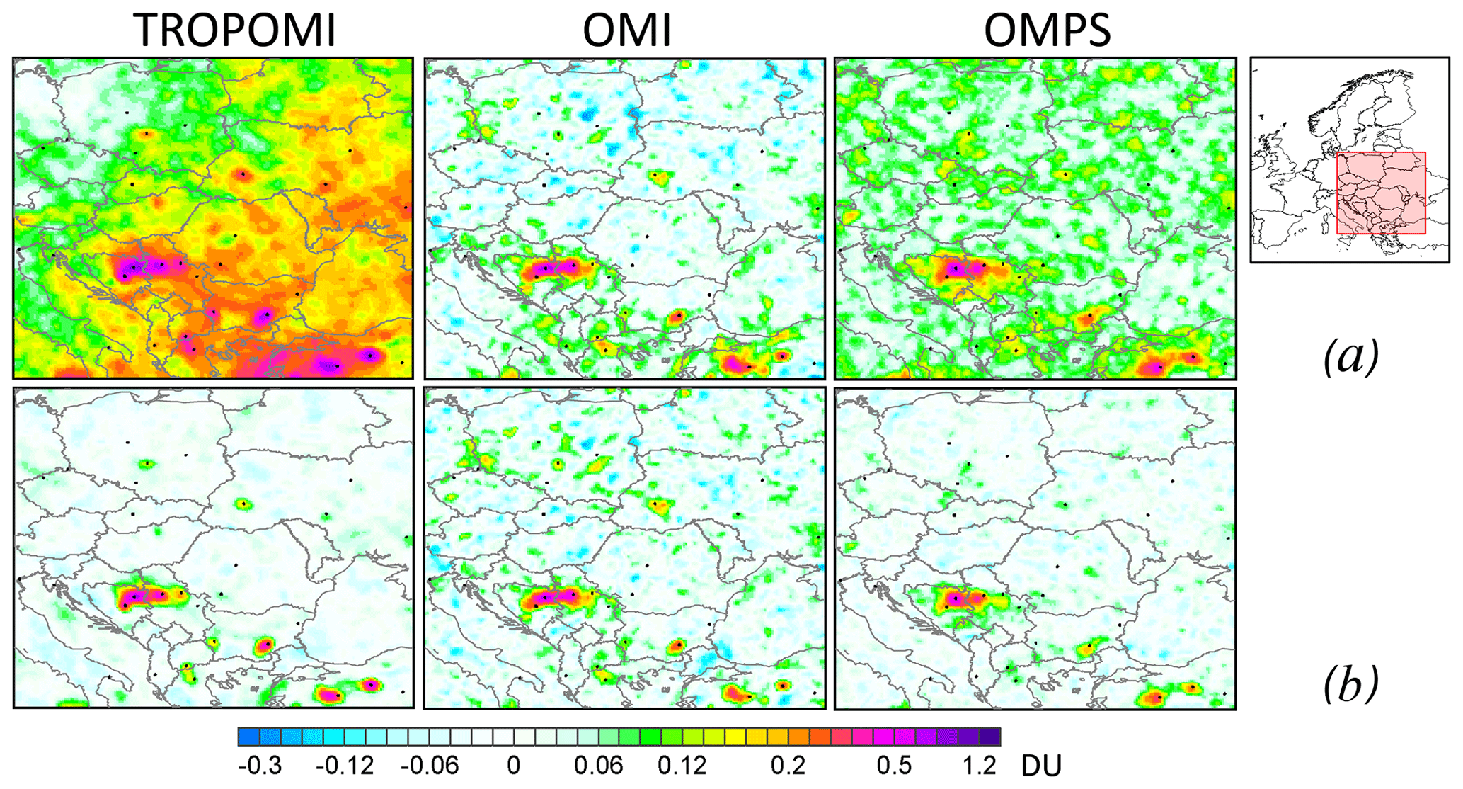
Figure 5 TROPOMI, OMI, and OMPS mean SO₂ over eastern and southern Europe for the period from April 2018 to March 2019 (a) and the same data but with large-scale biases removed (b). Data are smoothed by oversampling/pixel averaging with R=30 km. The black dots indicate the SO₂ emissions sources.

The problem of biases in TROPOMI data, as well as in the data from other satellites, requires further investigation and probably improvements of the SO₂ algorithms. In the case of TROPOMI, we saw such biases over many major areas of interest: China, India, Europe, and the Persian Gulf. The biases are often larger than the signals from emission sources, which creates an impression that TROPOMI values over such sources are larger than those from OMI. It also appears that the biases are larger in winter and fall than in summer and are also larger over water. It will be possible to investigate the time dependence of these biases as more TROPOMI data become available.

As mentioned, the uncertainties of TROPOMI data averaged over a certain area are 2–3 times smaller than those of OMI and OMPS. Due to its very high spatial resolution, in a single year TROPOMI can provide as much information on the SO₂ distribution around hotspots as OMI or OMPS can over several years. Figure 6 (top) shows the mean SO₂ over Bosnia & Herzegovina and Serbia in 2018 from OMI and TROPOMI and over the 2014–2018 period from OMI, using oversampling techniques (see Sun et al., 2018, and references therein). In these countries, SO₂ emissions were not under the same strict emissions-cutting regulations as in EU countries. Emissions from the power plants shown in Fig. 6 remained nearly constant between 2014 and 2018. A simple version of the oversampling technique was applied, in which a geographical grid was established around the source and the mean value of all satellite pixels centred within a 30 km radius from each grid point was calculated. As the mean is calculated, the standard error of the mean can also be calculated and used to evaluate the significance of that mean value by analyzing the ratio of the mean value to its standard error. Figure 6 shows both the mean values (the top row) and the ratios (the bottom row). Although individual TROPOMI SO₂ values are noisier than OMI values, the much larger volume of TROPOMI data contributing to the mean makes it appear less noisy than a 1-year OMI map, and only a 5-year OMI average demonstrates a TROPOMI-like level of noise. This is further confirmed by the ratio maps (Fig. 6, bottom): TROPOMI 1-year ratios are as high as 25, while OMI 1-year ratios are under 10 and only 5-year ratios are close to those for 1-year TROPOMI values.

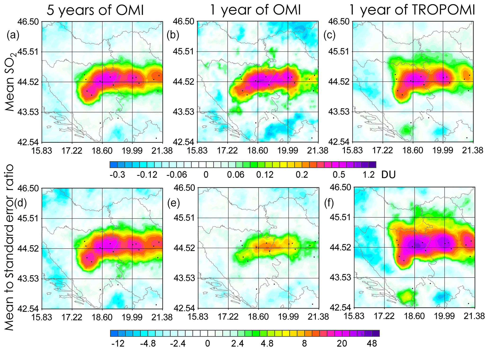
Figure 6 SO₂ hotspot over Serbia and Bosnia and Herzegovina: mean OMI values over a 5-year period (2014–2018) and mean OMI and TROPOMI values over a 1-year period (from April 2018 to March 2019). Data are smoothed by oversampling/pixel averaging with R=30 km. The constant bias is removed. The black dots indicate the emission sources. Panels (a–c) show mean SO₂ and panels (e–f) show the ratios of the mean SO₂ value to the standard error of the mean.

Although averaging multiple years of OMI data can produce the same or even higher signal-to-noise ratios as 1 year of TROPOMI data, OMI cannot provide the same level of detail as TROPOMI due to the difference in the instrument spatial resolutions. The high spatial resolution of TROPOMI also makes it possible to see individual sources in areas where multiple sources are in close proximity. As an example, Fig. 7 shows the mean SO₂ over a cluster of power plants in South Africa using 1 year of TROPOMI data and the entire (2005–2019) available record of OMI. For this plot, pixel averaging with a 10 km radius was used (smaller radii make the OMI map too noisy to see individual sources). Although we used a very small radius for averaging, it is hard to distinguish individual sources in the OMI map, while on the 1-year TROPOMI map they appear as local maxima or hotspots.

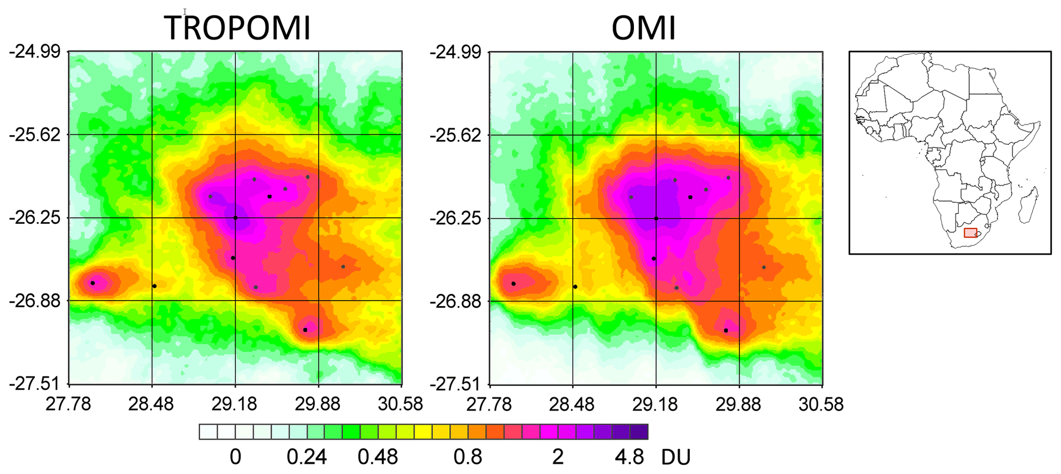
Figure 7 The mean TROPOMI SO₂ over a cluster of power plants in South Africa for the period from April 2018 to March 2019 and the mean 2005–2019 OMI SO₂ over the same region. Data are smoothed by oversampling/pixel averaging with R=10 km. The black dots indicate the emission sources. Note that the colour scale is different from the scale in the previous figures.

A high TROPOMI spatial resolution makes it possible in some cases to resolve an individual, persistent SO₂ plume. As an example, the mean SO₂ over Hawai`i for the period from April 2018 to March 2019 is shown in Fig. 8. The source, Kilauea volcano, is located at 1200 m above sea level, while the mountains north and northwest of the volcano are as high as 4000 m. The area is dominated by easterly winds. TROPOMI data demonstrate that, on average, elevated SO₂ values are not observed above the volcano peak. This means that the symmetrical, modified Gaussian plume model used for emissions calculations may not describe the actual plume very well in this particular case. OMI data with their lower spatial resolution do not really show these features of the SO₂ distribution.

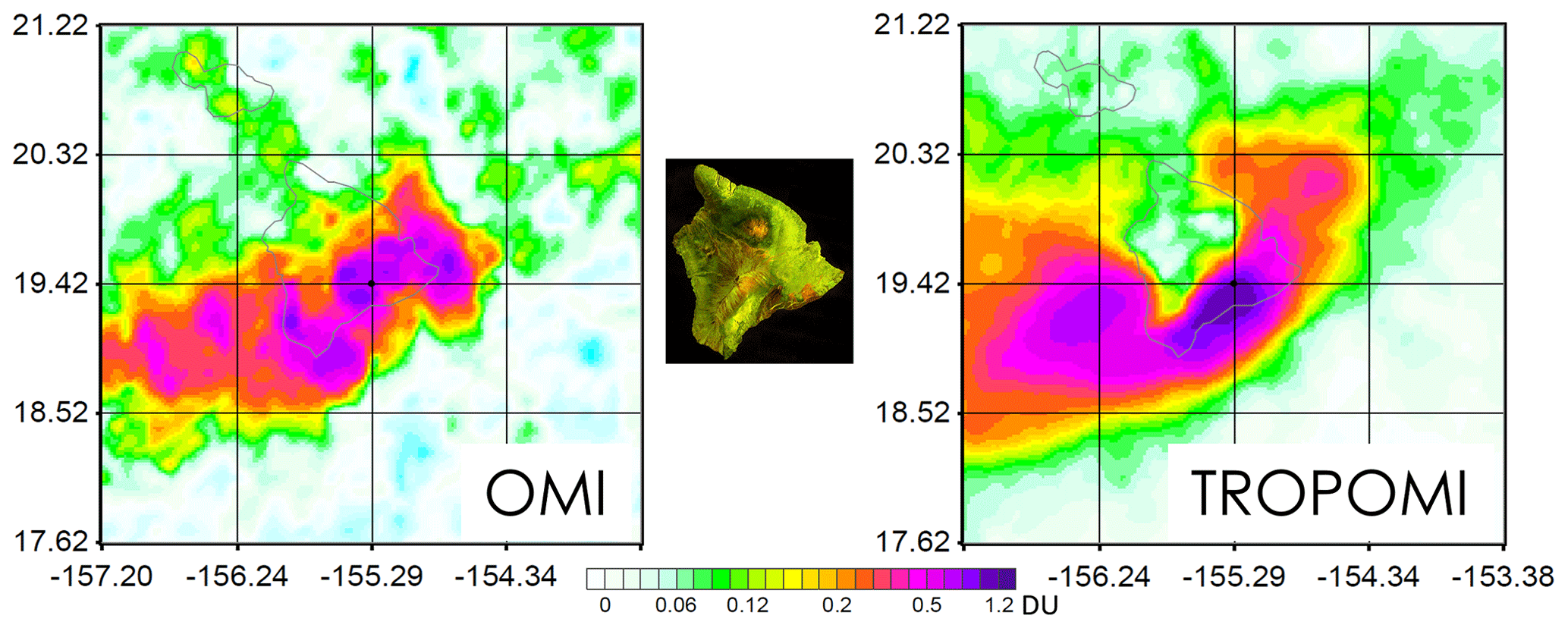
Figure 8 Mean SO₂ (DU) over Kilauea volcano, Hawai`i, from OMI and TROPOMI data for the period from April 2018 to March 2019. The volcano is in the centre of the map. The influence of orography on the SO₂ distribution is clearly visible due to the high spatial resolution of TROPOMI. A Sentinel-1 image from 23 May 2018 that illustrates the island's orography is shown in the middle of the figure.

4 Emissions estimates

A method developed to estimate emissions from point sources from OMI data (Fioletov et al., 2015) was applied here to TROPOMI, OMI, and OMPS data. The method is based on a fit of satellite data to an empirical plume model developed to describe the SO₂ spatial distribution near emission point sources. First, satellite measurements are merged with wind data and the rotation technique is applied (Pommier et al., 2013; Valin et al., 2013) so that the satellite data can be analyzed, assuming that the wind always has the same direction. Then, emissions and lifetimes were estimated using the exponentially modified Gaussian fit (Beirle et al., 2014; Fioletov et al., 2015; de Foy et al., 2015) appropriate for a near point source. The fitted plume model depends on three parameters: total mass (α) near the source; the lifetime or, more accurately, decay time (τ); and the plume width (σ). Finally, the emission strength (E) is calculated from τ by $E=\mathit{\alpha }/\mathit{\tau }$. For each source, all three parameters can be derived from a fit using a non-linear regression model, but when doing so the uncertainties in the non-linear parameters (τ and σ) are often large. To minimize this uncertainty, all emissions were derived using a mean τ and σ, determined by averaging over values obtained from the non-linear fits. Thus, only one parameter (α) is derived from the fit, which turns the algorithm into a simple linear regression model (Fioletov et al., 2016).

The three parameters for each of the three satellite instruments were estimated using April 2018–March 2019 data. It can be expected that the lifetime τ that characterizes the plume decay is the same for all three instruments. Indeed, we found that the average value of τ is about 6 h for all three of them. The plume width σ depends on the instrument pixel size and is expected to be different. We estimated that, as in the previous study (Fioletov et al., 2016), σ is about 20 km for OMI. For OMPS with its larger pixels, the average σ value is about 25 km. For TROPOMI, the average value of σ is about 15 km. However, many SO₂ sources are not really point sources. Industrial sources are often comprised of several individual facilities located a few kilometres apart. For example, in Norilsk, there are three major smelting factories located 8–10 km apart. For relatively large OMI pixels, this typically does not affect σ calculations. For TROPOMI, however, we can see that for real point sources σ is smaller, about 10 km, than for sources with multiple facilities. Our sensitivity study suggests that a change in sigma from 15 to 10 km reduces the emissions estimates by about 20 %. A better characterization of the emission sources will be required in the future in order to improve emissions estimates for sources with multiple facilities.

The calculations were performed in the same manner as the original study for OMI data (Fioletov et al., 2016). The parameter estimation was done using OMI pixels centred within a rectangular area that spreads ±L km across the wind direction, L km in the upwind direction and 3⋅L km in the downwind direction. As in the original study, the value of L was chosen to be 30 km for small sources (under 100 kt yr⁻¹), 50 km for medium sources (between 100 and 1000 kt yr⁻¹), and 90 km for large sources (more than 1000 kt yr⁻¹). For small sources, different L values have little effect on the estimated parameters, but smaller values of L allow the separation of individual sources where multiple sources are located in the same area. For larger sources, pixels with elevated SO₂ values are located over larger areas, and therefore the parameters estimated for higher L values have smaller uncertainties. Only pixels with associated wind speeds between 0.5 and 45 km h⁻¹ were used for the fitting. The overall uncertainty of the method is about 50 %. There are several factors that contribute to the emission estimate uncertainty; however, the major contributors, uncertainties in AMFs and τ, appear as scaling factors that affect TROPOMI-, OMI-, and OMPS-based estimates the same way. To remove the local biases mentioned above, the average SO₂ VCD for the area located upwind from the source was calculated and then subtracted from the data. As the biases may be different from season to season, all calculations were done for 3-month periods (seasons), and then the annual emission rate was calculated by averaging seasonal emission rates. Additional information about the algorithm and uncertainty analysis can be found in Fioletov et al. (2016).

We examined all sources listed in the catalogue (Fioletov et al., 2016) and calculated emissions for the period from April 2018 to March 2019 and their uncertainties using data from the three satellite instruments. It should be mentioned that although the catalogue contains about 500 sources, many were either closed or their emissions declined significantly due to several possible factors such as the installation of scrubbers and reduction in coal consumption. This includes most of the sources in the USA and the European Union and many sources in China. Volcanic degassing emissions also vary with time (Carn et al., 2017), and some of the volcanos that were active at the beginning of OMI operations did not emit high amounts of SO₂ in 2018–2019. Therefore, a decline in the number of catalogue sources detectable by TROPOMI is not entirely unexpected. The map of catalogue sources that are detectable from 1 year of TROPOMI data is shown in Fig. 9. The following criteria were used to identify a source as detectable: (a) the source should have an emission-to-uncertainty ratio exceeding 5 or (b) a ratio between 3.6 and 5 but with a clear hotspot at the source with a downwind tail. There are only 20 sites in the (b) category, and we examined them on a case-by-case basis. A total of 274 sites – including 147 power plants, 19 smelters, 40 oil-and-gas-industry-related sources, and 68 volcanos – with annual emissions from 10 to 2000 kt yr⁻¹ that satisfy these conditions were detected. They are listed in the Supplement.

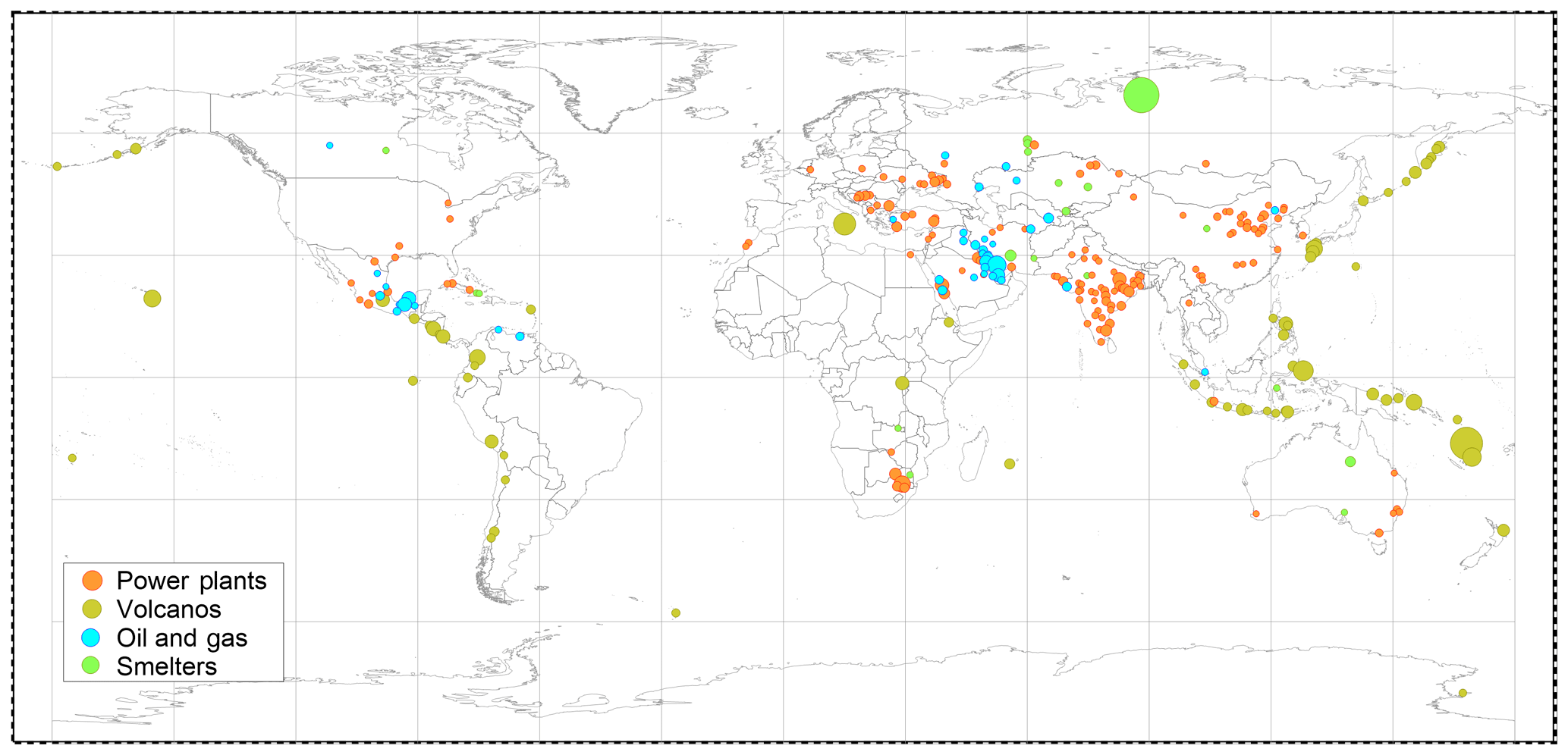
Figure 9 SO₂ emissions sources seen by TROPOMI in 2018. We checked ∼500 locations where OMI detected SO₂ emissions between 2005 and 2014 (Fioletov et al., 2016). Note that some of them are not active now or have had their emissions significantly reduced. TROPOMI can “see” 278 sites, including 150 power plants, 19 smelters, 41 oil-and-gas-industry-related sources, and 68 volcanos, with annual emissions from 10 to 2000 kt. The size of the symbols is proportional to the annual emission values.

Scatter plots of TROPOMI-, OMI-, and OMPS-based emissions estimates for all SO₂ catalogue sites are shown in Fig. 10a and b. Emissions estimates from OMI are on the horizontal axis of both panels. Both OMPS and TROPOMI emissions estimates show a good agreement with OMI estimates for sources with estimated emissions above 50–60 kt yr⁻¹ (calculated as an average of emissions estimates from the three instruments). For them, the correlation coefficients are about 0.97 for both instruments. However, the correlation coefficient is only 0.3 if calculated just for sources that emit less than 60 kt yr⁻¹. There are practically no systematic biases between estimates from the three instruments.

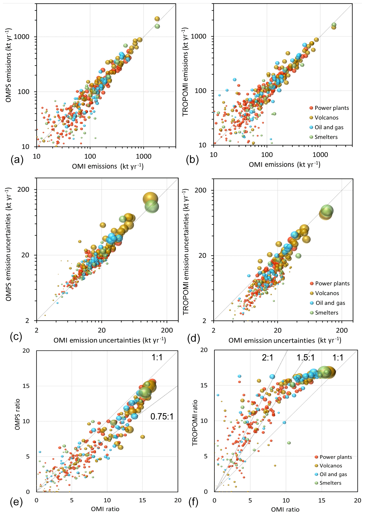
Figure 10 (a) Estimated OMI-, OMPS-, and TROPOMI-based emissions in kilotons per year. The bubble area is proportional to the ratio of emission to uncertainty. The bigger the bubble, the more reliable the estimate. (b) Emission uncertainties in kilotons per year. The bubble area is proportional to the emission rate. The bigger the bubble, the higher the emissions. (c) Ratios between estimated emissions and their uncertainties. The bubble area is proportional to the emission rate.

Not surprisingly, statistical uncertainties of the emissions estimates from the three satellite instruments are also highly correlated (Fig. 10c and d). In general, the OMPS-based emission uncertainties are slightly larger than those based on OMI data. The OMI-based emission uncertainties are almost always larger than those from TROPOMI data.

The relative TROPOMI emission uncertainties are lower than those from OMI. To illustrate that, Fig. 10e and f show scatter plots of the ratios of their signal-to-uncertainty ratios. For very large sources (> 1000 kt yr⁻¹), the emission-to-uncertainty ratio is dominated by SO₂ variability and not by the noise in satellite data. For example, SO₂ emissions from volcanic sources could be very different from day to day. Even if the emissions are fairly constant, different weather conditions (e.g. dry conditions vs. rain) affect the SO₂ dispersion patterns observed by satellites. For these very large sources, such SO₂ variability is larger than instrumental errors, and the emission-to-uncertainty ratio is nearly the same for all three instruments. For smaller sources, however, measurement uncertainties play a bigger role. For OMPS, the ratios are mostly below the 1:1 line, meaning that the uncertainties of OMPS-based emissions estimates are higher than those based on OMI data. It is the opposite for TROPOMI, where the ratios are mostly above the 1:1 line. Moreover, for medium-size and small sources, the ratios group around the 1.5:1 and 2:1 lines, meaning that the TROPOMI emissions estimate uncertainties are 1.5–2 times lower than those for OMI.

As all three satellite data sets can provide relatively independent emissions estimates, the present satellite-based SO₂ emissions inventory could be further improved by combining emissions estimates from the three sources. Due to its high resolution, and hence lower detection limit, TROPOMI can potentially identify many more sources than OMI and OMPS and then obtain emissions estimates for them. An exhaustive analysis of this is beyond the scope of this paper. However, as an example of the sizable advantage offered by TROPOMI, Fig. 11 shows the mean TROPOMI SO₂ distribution (from April 2018 to March 2019) at the border between Iran and Turkmenistan. The biggest source is the Khangiran gas refinery (1), an Iranian source that is included in the catalogue. The second largest source is located near Mary, Turkmenistan (2), and is related to gas exploration. The LANDSAT satellite images show that the source was built from 2012 to 2014. While 1 year of OMI data shows a signal from that region, they can hardly point to the source location. TROPOMI data clearly show a hotspot in both mean SO₂ (as shown) and the high signal-to-noise ratio (not shown) right at the source location. Moreover, there are two other sources that can be resolved by TROPOMI. One of them, located east of Khangiran, could be related to two power plants (Toos and Ferdosi (3)) that are 1 km apart. This source can also be used as an illustration of the difference in emission uncertainties between TROPOMI and OMI/OMPS. TROPOMI-based emissions estimates for this source are 14 kt yr⁻¹ with the standard error of 2.8 kt yr⁻¹, 5 times lower than the emission strength itself. The standard errors of OMI- and OMPS-based emissions estimates are 6.1 and 7.1 kt yr⁻¹, respectively, which is 2–3 times that of TROPOMI.

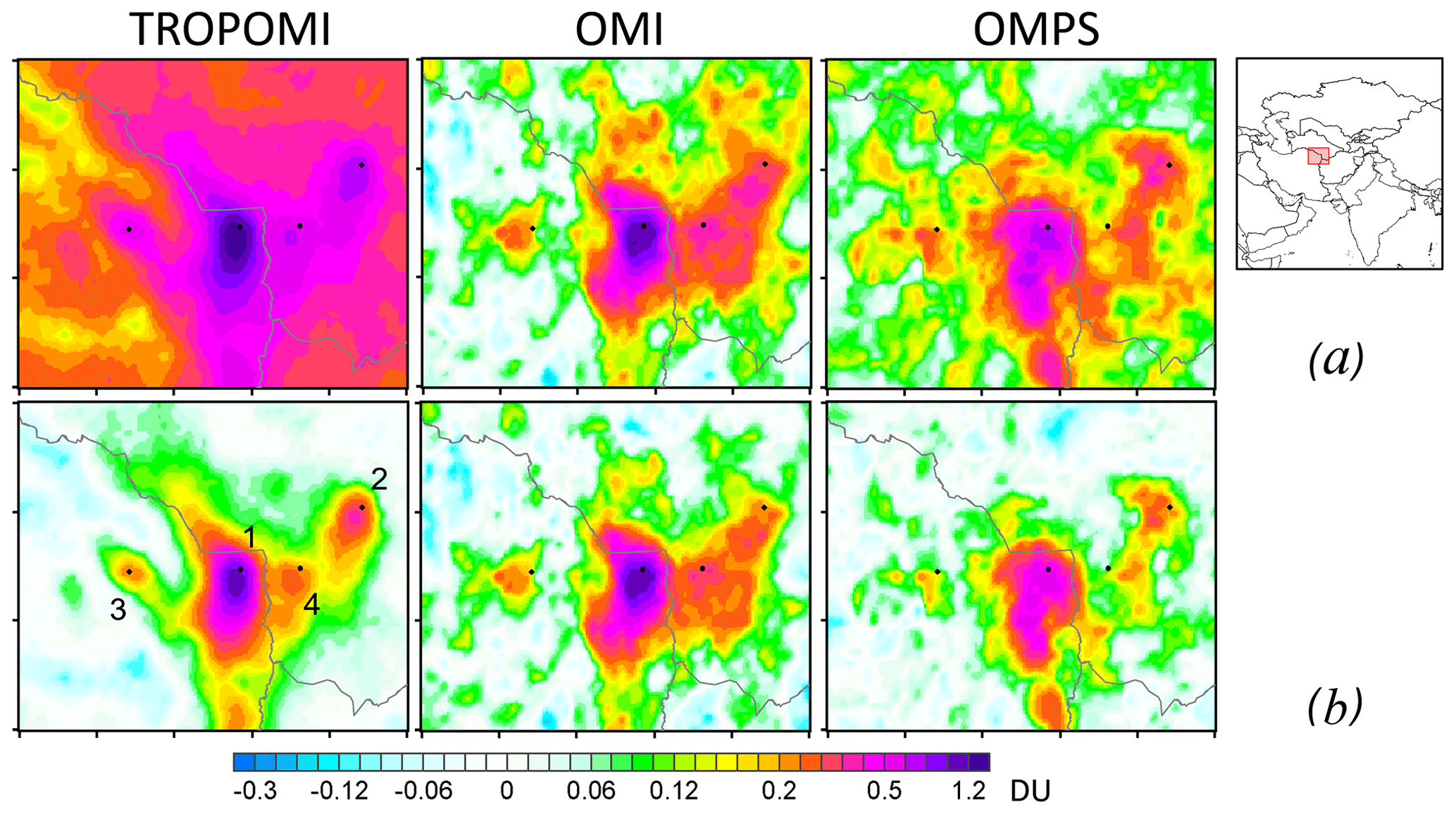
Figure 11 TROPOMI, OMI and OMPS mean SO₂ (DU) over the Khangiran region for the period from April 2018 to March 2019 (a). The same data, but with large-scale biases removed (b). Data are smoothed by oversampling/pixels averaging with R=20 km. The black dots indicate the SO₂ emissions sources: gas refinery at Khangiran, Iran (1); gas exploration sources at Mary (2) and Sovetabad (4), Turkmenistan; Toos and Ferdosi power plants, Iran (3).

5 Summary and discussion

The first analysis of TROPOMI near-surface SO₂ for the period from April 2018 to March 2019 reveals global distributions and features very similar to those seen from OMI and OMPS: elevated values over the Persian Gulf, India, and China; major hotspots over Norilsk, Russia, and South Africa; and major persistent volcanic sources such as Kilauea, Hawai`i, and Ambrym, Vanuatu. Outside the areas affected by these hotspots, all three instruments typically demonstrate low background SO₂ values within ±0.25 DU.

Over clean areas, the spatial standard deviations of TROPOMI data (about 1 DU over tropics and 1.5 DU over high latitudes) are larger than those of OMI (0.6–1 DU) and OMPS (0.3–0.4 DU) data. However, despite higher uncertainties of individual TROPOMI pixels, spatially averaged TROPOMI data over respective field of views have uncertainties that are 2–3 times smaller than those from OMI and OMPS data. As a result, annual mean SO₂ maps smoothed by spatial filtering appear less noisy than corresponding OMI maps. In terms of the signal-to-noise ratio, 1 year of TROPOMI smoothed mean values has the same uncertainties as 4–5 years of smoothed mean values based on OMI data.

We tested about 500 SO₂ sources previously detected from OMI data from 2005 to 2015; however, many of these sources emitted much less SO₂ in 2018 and 2019 than at the beginning of OMI operation. That includes, for example, almost all US sources and many sources in Europe and China. We were able to identify 274 sources where annual (from April 2018 to March 2019) emissions can be estimated from TROPOMI data. Their emissions are in the range from 10 to 2000 kt yr⁻¹.

Currently TROPOMI is able to provide point source SO₂ emissions estimates that have 1.5–2 times lower uncertainties than those from OMI, but it is less than expected, taking into account that the number of useful TROPOMI pixels is about 20 times higher than that of OMI. If the statistical uncertainties are inversely proportional to the square root of the number of averaged pixels and their uncertainties are the same, then it is expected that the standard errors for TROPOMI emissions estimates should be about 4–5 times lower than those for OMI. Taking into account that the SO₂ uncertainties of individual TROPOMI pixels are 1.5–2 times larger than those of OMI pixels, one can expect that TROPOMI emission uncertainties would be 2.5–3.3 times lower than OMI emission uncertainties, which is higher than the values of 1.5–2 that we derived directly from emissions estimates. This may suggest that errors in individual TROPOMI pixels are correlated, for example, due to large-scale biases.

There are larger-scale spatial biases in TROPOMI data over some areas that appear to be larger than similar biases in OMI and OMPS data. While the absolute magnitude of the biases is not very large (0.1–0.2 DU), it can be comparable to the SO₂ enhancements over large sources. Due to these biases, SO₂ values over some sources may appear larger in TROPOMI data than in OMI and OMPS data. If, however, such biases are removed by, for example, a statistical fitting procedure, TROPOMI annual mean SO₂ maps are very similar to OMI and OMPS maps. It also appears that these TROPOMI biases have a larger amplitude in winter and fall, although it is hard to say that this is a repeatable seasonal effect based on just 1 year of data.

Biases are very common in early versions of all satellite SO₂ products, and currently their origin is still not completely clear. The very small SO₂ absorption signal in the UV needs to be detected against a large contribution from ozone absorption. The latter is a strong function of stratospheric temperature (and hence ozone profile). Any imperfection in any of these parameters may yield a bias in retrieved SO₂. This, however, does not explain biases in the tropical region where ozone variability is low. Development of a PCA-type algorithm for TROPOMI could help to reduce these biases and improve the overall quality of the data. An improved version of the TROPOMI processing algorithm that includes a PCA component may produce a data product with smaller biases and lower noise than the present operational algorithm. Such an improved algorithm is now under development. Preliminary TROPOMI SO₂ retrieval tests applying a PCA-based algorithm have shown some promise, and work is underway to better understand algorithmic differences between DOAS and PCA.