Observational analysis of the daily cycle of the planetary boundary layer in the central Amazon during a non-El Niño year and El Niño year (GoAmazon project 2014/5)

The Amazon biome contains more than half of the remaining tropical forests of the planet and has a strong impact on aspects of meteorology such as the planetary boundary layer (PBL). In this context, the objective of this study was to conduct observational evaluations of the daily cycle of the height of the PBL during its stable (night) and convective (day) phases from data that were measured and/or estimated using instruments such as a radiosonde, sodar, ceilometer, wind profiler, lidar and microwave radiometer installed in the central Amazon during 2014 (considered a typical year) and 2015 during which an intense El Niño–Southern Oscillation (ENSO) event predominated during the GoAmazon experiment. The results from the four intense observation periods (IOPs) show that during the day and night periods, independent of dry or rainy seasons, the ceilometer is the instrument that best describes the depth of the PBL when compared with in situ radiosonde measurements. Additionally, during the dry season in 2015, the ENSO substantially influenced the growth phase of the PBL, with a 15 % increase in the rate compared to the same period in 2014.

1 Introduction

The Amazon basin covers about a third of the South American continent and extends for approximately 6.9×10⁶ km², of which about 80 % is covered by tropical forests (Tanaka et al., 2014; Ghate and Kollias, 2016). The Amazon biome represents more than half of the world's remaining tropical forests and consequently has a strong impact on the climate of South America. Thus it is one of the major tropical convective regions in the global climate system (Tang et al., 2016). It provides moisture to the global hydrological cycle and energy to drive the global atmospheric circulation, with a large influence on meteorological components such as the planetary boundary layer (PBL). Understanding convective systems over the Amazon region through observations is important for understanding and simulating these systems.

In this region there is a substantial quantity of convective activity that occurs during the entire year, but there are significant seasonal differences due to annual variation in atmospheric circulation and thermodynamic structure (Marengo and Espinoza, 2016), and these wet (or rainy) and dry seasons are well-defined. In this context, during the years 2014 and 2015, in the central Amazon region, the Green Ocean Amazon (GoAmazon) project was conducted with the objective of observing the influence of the complex interaction between the pollution plume generated in the city of Manaus-Amazonas and clouds and vegetation (Martin et al., 2016). This project approached research questions from a multidisciplinary perspective, and one of the studied topics was the physics involved in convective processes in the Amazon with emphasis on differences between wet and dry seasons.

The PBL is a turbulent layer of the atmosphere near the surface that results from the interaction between the surface and the atmosphere. The knowledge of the properties of the PBL has important scientific and practical applications because through this understanding of the PBL operational models of weather and climate forecasting can be refined, pollutant dispersion processes can be adequately described, the eolic potential of a region can be objectively determined, patterns of ventilation in urban areas can be estimated and improvements in agricultural techniques can be made (Englberger and Dörnbrack, 2017). Furthermore, a more realistic representation of processes that occur in the PBL can benefit numeric models of weather forecasting with better parameterization of convection, clouds and rain (Holtslag et al., 2013). The PBL characteristics, related to surface processes, provide important information regarding the priming of the atmosphere for convective initiation (Tawfik and Dirmeyer, 2014).

Holtslag et al. (2013) state that the PBL, since it is the lowest level of the atmosphere, is in continuous interaction with the Earth's surface, with significant turbulent transfer of heat, mass and momentum. According to these authors the PBL presents, during its daily cycle, large variations in temperature, wind and other variables in response to atmospheric turbulence and convective processes that occur in a tridimensional and chaotic form on timescales that range from seconds to hours, and the length across which these events occur is between a few millimeters and the entire depth of the PBL (1–2 km) or more in the case of convective clouds.

Neves and Fisch (2015) emphasize that an important characteristic of the PBL is the determination of its height because it is then possible to estimate the volume into which the source of pollution will be dispersed, and this is an important parameter for modeling of atmospheric dispersion. During its daily cycle the PBL undergoes atmospheric processes generated by thermal and mechanical convection during the day and displays stable conditions at night. The height of the PBL during the atmospheric instability phase (principally during the day) is called the convective boundary layer (CBL), and that during the stable period (principally at night) is named the nocturnal boundary layer (NBL).

In this context, observational evaluation of the daily cycle of the PBL, with emphasis on the CBL and NBL, represents an important field of study since within the PBL there occur processes that have a large impact on society and the terrestrial environment. Therefore, the objective of this study was to contribute to a more thorough understanding of the daily cycle of the height of the PBL through integration and comparison of data that were measured and/or estimated using instruments such as a radiosonde, sodar, ceilometer, wind profiler, lidar and microwave radiometer installed by the GoAmazon experiment. Furthermore, this study attempted to verify if the observational methods were representative of the daily variation in the cycle of the CBL and NBL in the central Amazon during 2014 (stated as a normal year) and 2015 and to elucidate the influence of an intense El Niño–Southern Oscillation (ENSO) event that occurred in 2015/2016.

2 Materials and method

In order to conduct this observational study, data from the GoAmazon project 2014/5 were used. The article by Martin et al. (2016) describes the details of the experiment wherein these data were collected, its principal objectives and some results. These data were collected using the structure that was installed at a research station called T3 (03^∘12^′36^′′ S, 60^∘36^′00^′′ W), located north of the municipality of Manacapuru in the state of Amazonas, about 9.5 km from an urban area and about 11.5 km from the left bank of the Solimões River, at the confluence of the mouth of the Manacapuru River (Fig. 1) in the central region of the Amazon basin. The T3 station is located in an area of pasture, surrounded by native forest with about 35 m of canopy height (Martin et al., 2016).

Figure 1 Location of the atmospheric measurement experiments in Manacapuru, Amazonas, Brazil.

At the experimental site of the T3 station, instruments were installed to obtain measurements of the hydrological cycle, PBL energy flux and other micrometeorological variables, and the data from these measurements are available on the web site of ARM – Climate Research Facility (https://www.arm.gov, last access: 1 June 2019). For the current study, four intense observation periods (IOPs) were defined in order to capture the peak of the rainy (February and March) and dry (September and October) seasons of 2014 and 2015. The dates for each IOP are 15 February to 31 March 2014 and 2015 for IOP1 and IOP3 and from 1 September to 15 October 2014 and 2015 for IOP2 and IOP4. For the daily cycle analysis of the PBL the sunrise was considered to be at 06:00 LT and the sunset was considered to be at 18:00 LT, not varying throughout the year.

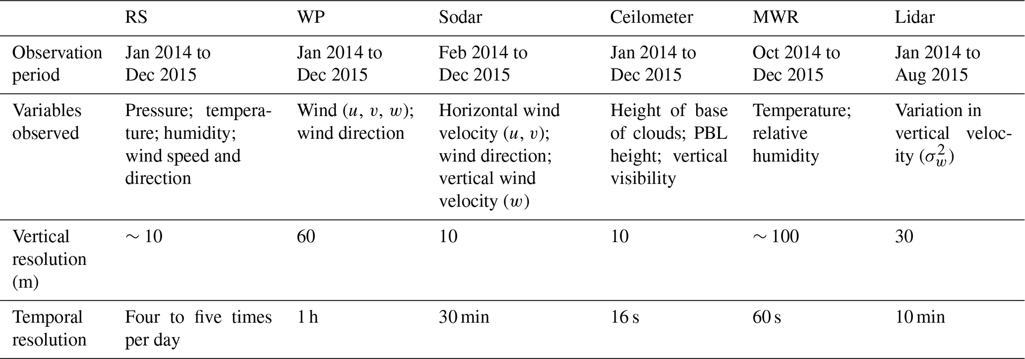
In order to measure the height of the PBL, instruments that probe the lower troposphere including a wind profiler (WP), ceilometer, sodar, microwave radiometer profiler (MWP) and lidar were used, and these data were compared to data taken in situ obtained using radiosondes (RSs), and this method is described below.

2.1 Radiosonde (in situ) – RS

In this experiment, RS measurements were obtained using a system that included a DigiCORA (MW12) (Vaisala Inc., Finland) with radiosonde model RS92SVG. The RS was coupled to a meteorological balloon that had an average ascension rate of 5 m s⁻¹, and the readings were taken at 02:00, 08:00, 14:00 and 20:00 local time (LT), and during IOP1 and IOP2 an extra RS was performed at 11:00 LT to better characterize the convective phase. From the RS measurements, the following data were measured as functions of time during a free-balloon ascent: pressure (hPa), air temperature (dry bulb) (^∘C), relative humidity (%), wind velocity (m s⁻¹) and wind direction (deg). With these measurements, other derived quantities were computed and used in this study: altitude (m), geographic position (latitude and longitude), dew point temperature (^∘C), u component of wind velocity (m s⁻¹) and v component of wind velocity (m s⁻¹).

From these data, the potential temperature (θ) and specific humidity (q) were extrapolated and their vertical profiles were used for the determination of e height of the PBL. At the CBL phase, the heights were identified by the vertical level where there was a systematic increase in potential temperature and a sudden reduction in specific humidity, and this method is called the profile method, as described in detail by Santos and Fisch (2007), Seidel et al. (2010), and Wang et al. (2016). However, at the NBL phase, the heights were determined by the height where the vertical θ gradient was null or less than a defined number (0.01 K m⁻¹) starting from the surface. This statement relates the maximum distance from the surface where the radioactive night cooling operates, as described in detail by Santos and Fisch (2007) and Neves and Fisch (2011).

2.2 Wind profiler (WP)

In order to construct a wind profiler (WP) at the study site, a radio acoustic sound system (RASS) model RWP915 from Vaisala Inc. (Finland) was used for direct and continuous measurements of the PBL. The WPs are Doppler instruments used to detect the vertical wind profile, and they function at a frequency of 50 MHz to 16 GHz. The WP–RASS installed at the study site operates at 915 MHz to measure the wind profile. The RASS transmitter aids in the measurement of the profiles of the vertical temperature. The WP–RASS operates through transmission of electromagnetic waves in the atmosphere and measures the intensity and frequency of the backscatter of the waves, assuming that atmospheric dispersion elements are moving with the average wind profile.

Since this is an instrument that operates at a high frequency and using smaller intervals of space between layers, it is frequently used for tropospheric observations, especially for the PBL. The method used in this study is described by Wang et al. (2016), wherein the height of the PBL was estimated using the vertical profile of electromagnetic refraction of WP, where the maximum of this index occurs in the upper part of the PBL.

2.3 Sodar

In the study area a mini-sodar (sound detection and ranging) (model Sodar MFAS and RASS A032002, Scintec, Rottenburg, Germany) was installed. This monostatic equipment consists of an emission-receiving antenna with an area of 1.96 m² and functions at a power of 10 W and a frequency of approximately 2 kHz. Using the sodar, profiles of wind velocity and direction were obtained at intervals of 30 min at a maximum height of 400 m.

Through remote sensor measurement by the sodar the height of the PBL was calculated for its night phase (nocturnal boundary layer, NBL) through the determination of the maximum wind height (jet). This method was suggested by Neves and Fisch (2011) and showed good results for the Amazon due to its operational limit (400 m) and taking into account that the NBL in the region has an average depth of 100 to 300 m.

2.4 Lidar

Lidar was also used to estimate the height of the PBL using a lidar model Stream Line^XR from Halo Photonics (Worcestershire, UK), a single autonomous instrument from the most recent line of products from this company for atmospheric remote sensing. These systems are adequate for meteorological studies of the PBL and also for measurements of cloud cover, vertical wind profiles and air quality monitoring (Gouveia et al., 2017).

These instruments employ a laser transmitter operating at a wavelength of 1.5 µm, low pulse energy (∼100 µJ) and high pulse repetition frequency (15 kHz). These instruments have full upper-hemispherical scanning capability and provide range-resolved measurements of attenuated particle backscatter coefficient and radial velocity. The fundamentals of its operation are similar to those of radar in which pulses of energy are transmitted to the atmosphere; the energy that is bounced back to the receiver is collected and measured as a resolved signal in time (Newsom, 2012).

Lidar uses a technique of heterodyne detection (method of extraction of coded information as a phase modulation and/or the frequency of a wavelength) in which the return signal is mixed with a reference laser beam (a local oscillator) of a known frequency. A computer within the instrument then processes the signal determining the Doppler frequency change using the spectrum from the signal. The energy content of the Doppler spectrums can also be used to determine attenuated backscattering.

Lidar operates in the near-infrared wavelength and is sensitive to retro-diffusion of aerosols at the micrometer scale; therefore it is capable of measuring wind speeds under clear-sky conditions with very high precision (normally 10 cm s⁻¹). Lidar also possesses a superior capacity for hemispheric sweeping, thus permitting tridimensional mapping of turbulent fluxes within the PBL. Using the variance of the vertical wind speed (${\mathit{\sigma }}_w^{\mathrm{2}}$) provided by the lidar, the method of Huang et al. (2017) was employed, where the authors define the depth of the PBL as a layer in which ${\mathit{\sigma }}_w^{\mathrm{2}}$ exceeds a specific limit (0.1 m² s⁻²).

2.5 Ceilometer

The PBL was also monitored using a ceilometer model CL31 from Vaisala Inc. (Finland). The Vaisala ceilometers are a type of lidar remote sensing instrument that operate through a maximum vertical range of 7700 m and register the intensity of optical backscattering at the near-infrared wavelength between 900 and 1100 nm through the emission of a vertical pulse that is autonomously executed. These measurements are used to produce derived products that are recorded: the height of the cloud base, the retrieval of the particle backscatter coefficient and PBL height (Wiegner et al., 2014; Shukla et al., 2014; Morris, 2016; Geiß et al., 2017; Carneiro et al., 2020). Although the ceilometer measures the reflection of the aerosol layer (thus the mixing layer height), it was assumed to be the diurnal PBL height since the entrainment zone is very shallow. Thus, throughout this paper, this information (backscatter aerosols) was assumed to be PBL height. The ceilometer is a high-temporal-resolution instrument with a measurement interval of 2 s and a sampling rate of 16 s, and it is a powerful tool for measuring the height of the PBL during its daily cycle (day and night phases) to a high level of detail. The ceilometer signal results from light backscattered by particles at the atmosphere; the intensity of backscattering depends on the concentration of particles in the air (Morris, 2016). Ceilometers use pulsed diode laser lidar (light detection and ranging) technology to determine the attenuated backscatter, and the particle backscatter coefficients are obtained from these data. Subsequently the heights of the cloud base and the PBL are calculated (Wiegner et al., 2014; Kotthaus et al., 2016; Morris, 2016; Geiß et al., 2017).

The standard procedure for the PBL heights determination from Vaisala ceilometers is the software package BL-View developed by the manufacturer (see more details in Morris, 2016; Geiß et al., 2017; Geisinger et al., 2017).

2.6 Microwave radiometer profiler (MWR)

Data were also used from a microwave radiometer profiler model MP3000A from Radiometrics Corp., Boulder, CO, USA. This instrument provides vertical profiles of temperature, humidity and liquid water content at a sampling rate of 60 s and average values at intervals of approximately 5 min. The profiles are deduced from measurements of radiance values of absolute microwaves (expressed as “brightness temperature”) obtained at 12 different frequencies at intervals of 22–30 and 51–59 GHz. This type of data are useful as input into numerical models of weather forecasting which need high-resolution profiles in continuous time.

To obtain the potential temperature throughout the daily cycle, it was necessary to interpolate the pressure profiles of the RS using to the method of polynomial interpolation. Together with the MWR air temperature profiles, the daily cycle of the potential temperature profile was calculated. Thus, the height of the PBL was estimated using the profile method.

Table 1 This table presents a synthesis of the instruments used in this study, the observation periods, and temporal and spatial resolutions.

The remote sensor instruments capture multiple layers from the heights of the PBL in the transition interval of day to night (between 17:00 and 18:00 LT) shown in Fig. S1 (presented in the Supplement). However, as one of the goals of this paper is to have a complete picture of the PBL cycle, the NBL heights in this interval were neglected in Figs. 4 and 6, in order to show only the decay of the CBL convection.

Determination of monthly rainfall for both study years was carried out using data taken with a disdrometer model Parsivel² (OTT Hydromet GmbH, Germany), with a temporal resolution of 10 min. Measurements of turbulence flows were used for the eddy covariance (EC) system composed of a three-dimensional (3-D) sonic anemometer (model WindMaster Pro, Gill Instruments Limited, Hampshire, UK) coupled with an open-path infrared gas analyzer (IRGA) (LI-7500, LI-COR Inc., Lincoln, Nebraska, USA) at 10 m above the ground. The EC provides an estimate of the net exchange of energy and mass between the terrestrial surface and the atmosphere. The estimated flux is given by a scalar magnitude that is defined as the average of the product of the fluctuations of the vertical velocity and the concentration that is being transported. In practice, this technique consists of taking observations of variables of the product at a high frequency (10 Hz), and from this large number of samples of each variable the statistical covariation is calculated between them. In this manner the system provides in situ measurements of turbulent fluxes of momentum, sensible and latent heat, and carbon dioxide to the surface.

The measurements of radiation and soil heat flux were taken every 30 min using the Surface Energy Balance System (SEBS), which consists of measurements of solar and terrestrial radiation collected using radiometers, and the radiation balance by a net radiometer model CNR4/CNF4, (Kipp & Zonen, Delft, the Netherlands) installed 2 m above the ground. There was a coupling of sensors measuring soil heat flux by flux plates (HFT-3, Hukseflux Thermal Sensors, Delft, the Netherlands) buried at 0.02 m depth in this system.

In the results obtained, the average and standard deviation values were computed for different time intervals along the PBL daily cycle (Tables 2 and 3). The computed Pearson's correlation coefficient (r) showed values higher than 0.6 for all remote sensors related to the RS, especially for the ceilometer, which showed correlations around 0.8. Also, a significant statistical test (Student's t test with 95 %) was applied for the 45 d of each IOP, with 2 degrees of freedom, and the results showed that there is statistical significance between the remote sensors and RS (Tables S1 to S4 in the Supplement).

3 Results and discussion

Analysis of the meteorological variables revealed that accumulated precipitation was different between years (Fig. 2). The year 2014 was similar to the normal climatology (for the city of Manaus – data extracted from INMET, 2018) for the region (2300 mm), with a total of 2451 mm. This high rate of rainfall can be understood as a response of the dynamic fluctuation of the nearly permanent center of convection, associated with a high rate of local evapotranspiration, which contributed to recycling of water vapor and rainfall (Nobre et al., 2009; Rocha et al., 2017). In contrast, the year 2015 registered a significant reduction (approximately 30 %) of the total rainfall in relation to the previous year, with a total accumulation of 1764 mm, well below the normal climatological average. This reduction is associated with the occurrence of the El Niño–Southern Oscillation (ENSO) event of that year (ECMWF, 2017; Macedo and Fisch, 2018; Newman et al., 2018).

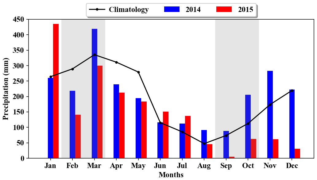
Figure 2 Distribution of accumulated monthly precipitation (mm) for the years 2014 and 2015 and the normal climatological pattern.

During 2014, monthly accumulated precipitation was always above 50 mm per month, and during representative months of IOP1 (February and March 2014) the total accumulated precipitation was 720 mm. However, during IOP2 (September and October 2014) the total accumulated precipitation was 185 mm, yielding a reduction of nearly 75 % of accumulated precipitation during IOP1. According to Ferreira et al. (2005), this difference between the rainy and dry seasons occurs because rainfall distribution in the Amazon is very irregular, with high spatial and temporal variability. Marengo et al. (2017) provide a more detailed explanation of this characteristic of central Amazonia and include the large-scale forcing role in the description of rainfall during the rainy and dry seasons.

While 2015 had a large reduction in rainfall, during the months of the period of intense observation of the rainy season (IOP3) the accumulated precipitation was 398 mm, representing a reduction of approximately 50 % of the total accumulated precipitation during the rainy season of 2014 (IOP1). During IOP4, the total accumulated precipitation was well below the normal climatological value, as well as in comparison to the same period in 2014 (IOP2), with a total registered precipitation of 68 mm, a reduction of approximately 65 % compared to IOP2. This occurred due to the EN event being more intense during these months (ECMWF, 2017; Newman et al., 2018). The ENSO event (2015/2016) was considered one of the most intense in recent years, with an intensity similar to that which occurred during 1982/83 and 1997/98 (ECMWF, 2017).

3.1 Typical year (2014)

Daily cycles of 30 min averages of the components of the balance of energy are presented in Fig. 3 for IOP1 (Fig. 3a) and IOP2 (Fig. 3b) for 2014. The shaded area for Fig. 3 which represents the standard deviations values was computed for each 30 min time interval. It is also shown in Figs. 4 to 6.

In these figures, the radiation balance (R_n) had positive values between 06:00 and 18:00 LT, with 455 W m⁻² for IOP1 at 12:00 LT, and IOP2 had greater intensity of R_n with 534.5 W m⁻² at 11:00 LT.

The latent heat flux (LE) showed that the majority of the available net radiation (daytime conditions) was used for this flux. Both periods had similar maximum values, with 355.9 (IOP1) and 350 W m⁻² (IOP2) at 12:00 LT. However, there was a reduction of net radiation converted into LE between the periods, with 75 % in IOP1 and 66 % in IOP2. Since IOP2 refers to the dry season in the region, this presented lower water availability in the system (surface–atmosphere), which resulted in the lowest LE∕R_n partition in comparison to IOP1.

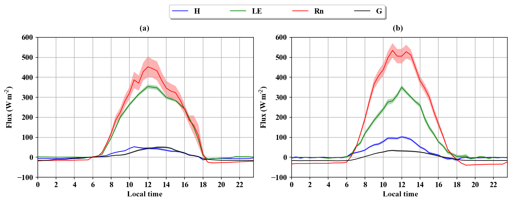
Figure 3 Average daily cycle of the radiation balance (R_n) (W m⁻²), sensible heat flux (H) (W m⁻²), latent heat flux (LE) (W m⁻²) and soil heat flux (G) (W m⁻²) during IOP1 (a) and IOP2 (b). The shaded area represents the standard deviation.

In the Amazon, especially during the rainy season, only a small fraction of R_n (about 10 %) is transformed into sensible heat flux (H), and this maximum of 52 W m⁻² occurred at 10:30 LT during IOP1, while for IOP2, due to lower precipitation values and soil moisture deficit, there was an increase of 21 % in the fraction of R_n transformed into H, with a maximum of 112.8 W m⁻² at 12:00 LT.

Nevertheless, only a small percentage of R_n is converted into heat flux in the soil (G), with a maximum of 50 W m⁻² for both IOPs. These results showed that independent of the season, this flux is always low and is limited to about 5 % of the total available energy.

Figure 4 shows the hourly average of the heights of the PBL for the IOP1 (Fig. 4a) and IOP2 (Fig. 4b), and Table 2 shows standard deviations values in different time intervals along the PBL daily cycle. The sunrise and sunset times were marked by the vertical lines of 06:00 and 18:00 LT, respectively, since the study area is close to the Equator line and there are not changes at these times. The RS (in situ measurements) was considered the truth depth of the boundary layer, while the others presented were estimated by remote sensing.

Figure 4 Daily cycle of the height of the PBL during the IOP1 (a) and IOP2 (b) experimental periods. The vertical lines represent sunrise (06:00 LT), sunset (18:00 LT) (full line) and NBL erosion (dashed line). The shaded area represents the standard deviation.

During the phase in which the NBL is formed (between 00:00 and 06:00 LT), IOP1 showed small vertical oscillations of its depth due to the occurrence of sporadic rainfall (Fig. 4a). The results obtained from the ceilometer between 00:00 and 03:00 LT showed that the depth of the PBL varied between 180 and 280 m, and after 04:00 LT there was an increase in the maximum height to 350 m, which was reduced in the following hours to 275 m by 06:00 LT (sunrise).

The measurements made with the WP also showed some oscillations in the height of the NBL, with a reduction in height between 00:00 and 02:00 LT from 280 to 250 m and then an increase to a maximum of 350 m at 04:00 LT, remaining constant until 06:00 LT. The sodar results during this interval showed lower variation in NBL depth during this same interval. The variation observed from the measurements by the different sensors is related to intermittent mechanical turbulence which could be the result of the presence of clouds and rain on some days and not on others, thus provoking an increase in wind variability during the night, which has the effect of deepening the NBL. However, in this same interval during IOP2 (Fig. 4b) the NBL was very stable with an average height of 250 m for all sensors (ceilometer, WP, sodar, MWR and lidar), thus corroborating the explanation of the influence of rainfall on the determination of variability of depth of the NBL.

The results found for the height of the NBL were similar to those reported by Neves and Fisch (2011), in a study using sodar in the southwestern Amazon, where the authors observed NBL heights varying from 150 to 329 m. However, Acevedo et al. (2004), also studying in a pasture site in the Amazon (in Santarém-PA), observed lower NBL heights than those from the current study (between 50 and 150 m), and this difference occurs because of different geographic conditions (influence of river breeze, fog formation, etc.). As an example of these influences, in the Santarém region the authors observed several cases of formation of fog during the night, which was not observed at the pasture site in Rondônia (see Neves and Fisch, 2015) or at T3 the site.

Table 2 Standard deviation calculated for PBL height measurements of instruments at different intervals of the daily cycle.

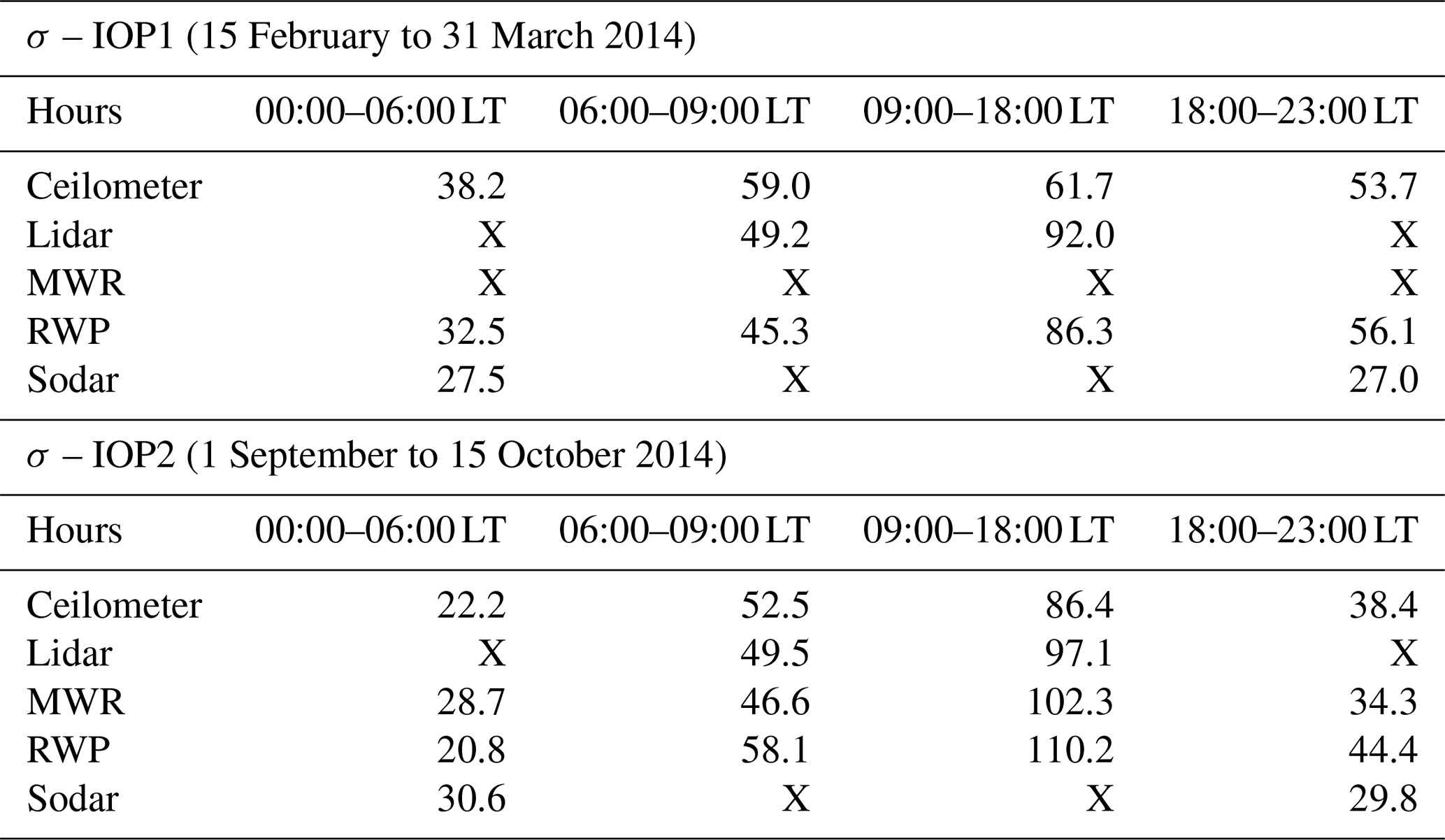
* “X” represents where absence measurements occurred.

The phase of the erosion of the NBL according to Stull (1988) begins after sunrise (at 06:00 LT in the Amazon), and the complete erosion of the NBL occurs when the whole layer is mixed. The potential vertical gradient is almost null and as a consequence there is a high growth rate (above 100 m h⁻¹). Thus, during this phase there are still several layers. In IOP1 (Fig. 4a), the erosion phase occurred 3 h after sunrise, where it was observed that in the first hours of this phase there is no increase in the PBL depth. Only after 08:00 LT did an increase in PBL height occur (average rate of 22.8 m h⁻¹). This occurs due to a lower H flux (Fig. 3a), which causes the erosion of the NBL to progress slowly, and total erosion occurs only at 09:00 LT when the average rate is 102 m h⁻¹.

In contrast, in the IOP2 (Fig. 4b), as a function of greater stability of the NBL and the positive values of R_n and H occurring earlier, initial erosion of the NBL begins at 06:00 LT, and there is a rapid increase in the depth of the PBL compared to IOP1. This increase continues in the subsequent hours at a rapid rate of 70.8 m h⁻¹, which causes the NBL to be completely eroded by 08:00 LT. This result demonstrates that the erosion of the NBL in this region is conditioned by greater availability of energy in the early hours of the morning and by how much of this energy will be used for heating of the atmosphere (H).

The transition from nighttime to daytime is very complex. Although the H has become positive (thus heating the atmosphere), this amount of energy did not completely warm the atmosphere and erode the NBL (see Figs. S3 and S4 in the Supplement).

In IOP1, after complete erosion of the NBL the development phase of the convective boundary layer (CBL) begins, and due to the slow erosion of the NBL the growth of the CBL begins at 11:00 LT with a typical height of 850 m and an average increase of 102 m h⁻¹, until it reaches its greatest depth at 1180 m at 13:00 LT. However, soon after the maximum is registered, the CBL presents a small reduction in depth (13.3 m h⁻¹), due to the low value of H, which did not exceed 50 W m⁻². This surface flux, added to the entrainment flux at the top of the CBL, was not sufficient to maintain turbulence in this layer, which showed a reduction after this time.

During IOP2, with the NBL being rapidly degraded, the CBL that subsequently formed had a more rapid development, with an average growth rate of 175.2 m h⁻¹. The CBL had a more prolonged phase, with the maximum depth of 1590 m registered at 13:30 LT. After this maximum of the CBL there was a slight reduction in its growth rate (−39.2 m h⁻¹) until 17:30 LT, when H returned to a null value. This depth is similar to that reported by Fisch et al. (2004) in a study of the CBL in a pasture in Rondônia in the southwestern Amazon, where the authors observed a maximum depth of 1650 m in the dry season. Neves and Fisch (2015) also observed in Rondônia that in the initial formation of the CBL during the dry season there was very rapid growth between 08:00 and 11:00 LT, with maximum heights of about 1500 m at 14:00 LT.

3.2 El Niño year (2015)

The energy fluxes for IOP3 (Fig. 5a) and IOP4 (Fig. 5b) show that during the 2015 rainy season, R_n IOP3 behaved in an analogous manner as in the rainy season of 2014 (IOP1), with a maximum of 488 W m⁻² at 12:00 LT. However, during the dry season of 2015 (IOP4) there was an increase in intensity compared to IOP2, with maximum R_n equal to 555.2 W m⁻² at 12:00 LT. This greater flux of net radiation to the surface will be converted into heat flux, meaning that there is greater energy available during the dry season of 2015 compared to that of 2014 due to less cloud cover, a common characteristic in years with ENSO events (Macedo and Fisch, 2018).

The LE registered a maximum of 310 W m⁻² during IOP3 at 12:00 LT. This result represented 65 % of the partitioning of R_n. These results are within the range of results for LE in this region, for which 70 % of R_n is generally converted into LE (Von Randow et al., 2004; Andrade et al., 2009). Due to the low the low water availability during IOP4, there was a reduction in the partitioning of R_n into the LE flux, only about 35 % in comparison with IOP3, resulting in a reduction of more than 50 %. The maximum LE registered was at 12:00 LT and was 179 W m⁻², while during IOP3 just 17 % of R_n was converted into H, with a maximum H of 86 W m⁻² observed at 13:00 LT. During IOP4, H had larger averages, and 60 % of R_n was converted into H, with a maximum of 280 W m⁻² at 12:00 LT. Furthermore, in 2015 during IOP3 and IOP4, only a small percentage of R_n was converted into G, with a maximum of 40.0 W m⁻² in IOP3 and 50.0 W m⁻² in IOP4, both at 12:00 LT.

Figure 5 Average of the daily cycle of net radiation (R_n) (W m⁻²), sensible heat flux (H) (W m⁻²), latent heat flux (LE) (W m⁻²) and soil heat flux (G) (W m⁻²) in the study region during IOP3 (a) and IOP4 (b). The shaded area represents the standard deviation.

The daily cycle of CBL during IOP3 (Fig. 6a), as well as in IOP1, showed vertical oscillations of the NBL's height (between 00:00 and 06:00 LT) of 200 m (00:30 LT) to 375 m (03:00 LT). The WP and the sodar yielded lower depths than the ceilometer and the MWR. However, during IOP4 (Fig. 6b) the NBL was more stable, with an average height of 250 m, similar to what was observed during IOP2. The result from 00:00 to 06:00 LT confirms that in the Amazon region the NBL is more stable during the dry season compared to the rainy season, when it has larger variation in its depth. Table 3 shows standard deviation values in the different time intervals.

Figure 6 Daily cycle of the height of the PBL during the IOP3 (a) and IOP4 (b) experimental periods. The vertical lines represent sunrise (06:00 LT), sunset (18:00 LT) (full line) and NBL erosion (dashed line). The shaded area represents the standard deviation.

The IOP3 demonstrated a similar erosion pattern for the NBL to that observed during IOP1, with the NBL still established between 06:00 and 08:00 LT. From this time onward there was an increase in depth of the CBL with an average growth rate of 19.6 m h⁻¹. In this manner, just as in IOP1, the erosion of the NBL during IOP3 occurred slowly, with total degradation at 09:00 LT. This result is similar to that which was observed during the same phase in IOP1, where the NBL was less stable and together with lower availability of energy at the surface caused a slower erosion of the NBL. However, the erosion phase during IOP4, in response to an increase in R_n and H, occurred earlier (06:00 LT). Additionally, during the dry season of 2015, the rate of ascension was higher during the subsequent hours and reached 76.1 m h⁻¹, such that the NBL was completely eroded at 08:00 LT.

The development during IOP3 occurs in an analogous manner to that observed during IOP1, with weak vertical development of the maximum depth. At 10:00 LT the CBL begins to develop and has a height of 830 m and a growth rate of 100.3 m h⁻¹, reaching a maximum depth of 1069 m (13:30 LT), demonstrating a shallower CBL during the wet season. However, in contrast to IOP1, IOP3 had a CBL established during the entire evening period, probably as a function of lower frequency of rainfall. IOP4, during the 2015 dry season, had greater development of convection after erosion at 08:00 LT, with a high growth rate of 193 m h⁻¹, and at 11:00 LT the CBL was completely established. With the CBL established as a result of greater heating of the atmosphere by H, there was greater depth of the CBL, reaching a maximum of 1925 m at 14:00 LT, and this was influenced by the strong EN event, which intensified the dry season in the region and caused the highest values of H. This caused greater thermal convection in the development of the CBL, which increased its depth by 21 % in relation to that observed in IOP2. This maximum depth of the CBL during IOP4 is not commonly found in studies conducted in the Amazon region before; however Lyra et al. (2003), using radiosonde data, reported a maximum height of 2200 m during the dry season of 1994 in Rondônia.

Table 3 Standard deviation calculated for PBL height measurements of instruments at different intervals of the daily cycle.

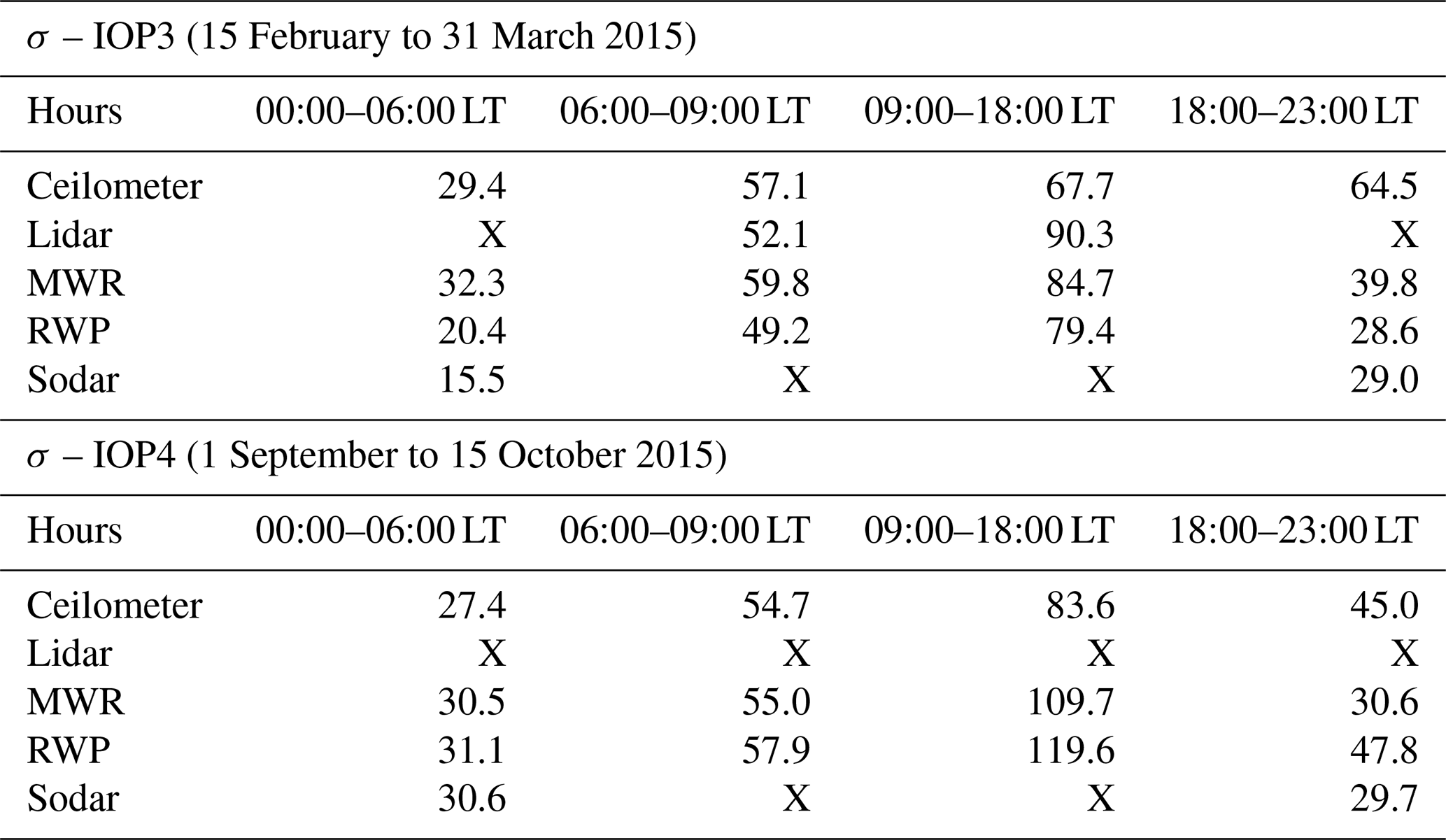
* “X” represents where absence measurements occurred.

4 Conclusions

During the four IOPs the results show that during daytime and nighttime intervals, independent of weather conditions, the ceilometer is a promising sensor with good accuracy for direct and continuous measurement of the height of the PBL (which on average ranged from 250 m – NBL to 1900 m – CBL) when compared to in situ RS. The RS, in spite of it being a proven high-precision method, in this experiment was launched only on synoptic times plus an extra at 15:00 UTC. Hence, it did not capture a high-temporal-resolution (like the remote sensors) daily cycle evolution of the height of the PBL, due to the long time interval between launches (each 6 h). While the MWR, WP and the lidar were satisfactory for estimates of the convective phase (CBL) of the PBL, during the nocturnal phase (NBL) these sensors overestimated heights. Additionally, the sodar under- and overestimated the NBL during these periods.

The intense EN event of 2015/2016 influenced the development phase of the CBL during the dry season of IOP4, and it had a growth rate of about 15 % higher than the results from IOP2 and a sensible heat flux (responsible for heating the air) that was higher than the standard values for the central Amazon. As a consequence, more intense convective movements occurred and contributed to a stronger vertical development of the layer.

The NBL erosion showed differences between seasons, presenting an erosion time of 2 h in the dry IOPs (2 and 4), and 3 h in the wet IOPs (1 and 3). A more detailed analysis of NBL erosion is being elaborated in Carneiro and Fisch (2020).