the Creative Commons Attribution 4.0 License.
the Creative Commons Attribution 4.0 License.
 | 05 May 2020
Nitrous acid (HONO) emissions under real-world driving conditions from vehicles in a UK road tunnel
Leigh R. Crilley
Thomas J. Adams
Stephen M. Ball
Francis D. Pope
William J. Bloss
Measurements of atmospheric boundary layer nitrous acid (HONO) and nitrogen oxides (NOx) were performed in summer 2016 inside a city centre road tunnel in Birmingham, United Kingdom. HONO and NOx mixing ratios were strongly correlated with traffic density, with peak levels observed during the early evening rush hour as a result of traffic congestion in the tunnel. A day-time ΔHONO∕ΔNOx ratio of 0.85 % (0.72 % to 1.01 %, 95 % confidence interval) was calculated using reduced major axis regression for the overall fleet average (comprising 59 % diesel-fuelled vehicles). A comparison with previous tunnel studies and analysis on the composition of the fleet suggest that goods vehicles have a large impact on the overall HONO vehicle emissions; however, new technologies aimed at reducing exhaust emissions, particularly for diesel vehicles, may have reduced the overall direct HONO emission in the UK. This result suggests that in order to accurately represent urban atmospheric emissions and the OH radical budget, fleet-weighted HONO∕NOx ratios may better quantify HONO vehicle emissions in models, compared with the use of a single emissions ratio for all vehicles. The contribution of the direct vehicular source of HONO to total ambient HONO concentrations is also investigated and results show that, in areas with high traffic density, vehicle exhaust emissions are likely to be the dominant HONO source to the boundary layer.
- Article
(1214 KB) - Full-text XML
-
Supplement
(537 KB) - BibTeX
- EndNote


Nitrous acid (HONO) is an important atmospheric constituent in the boundary layer, as its photolysis leads to the formation of OH radicals (Reaction R1), which drive atmospheric oxidation reactions, pollutant removal and the formation of secondary species. This is particularly important in urban areas where the measured HONO mixing ratios can reach up to parts per billion, and HONO photolysis can be the dominant HOx source (Alicke et al., 2002; Elshorbany et al., 2009; Kleffmann, 2007; Lee et al., 2016; Michoud et al., 2012; Villena et al., 2011).
The sources of HONO in the atmosphere can be primary or secondary (Fig. 1). Primary sources include direct emissions from combustion processes such as vehicle emissions (Kirchstetter et al., 1996; Liu et al., 2017; Rappenglück et al., 2013; Trinh et al., 2017; Xu et al., 2015), soil microbial activity (Laufs et al., 2017; Maljanen et al., 2013; Meusel et al., 2018; Oswald et al., 2013; Su et al., 2011) and biocrusts (Maier et al., 2018; Meusel et al., 2018; Weber et al., 2015). Secondary sources were thought to be dominated by the homogeneous gas phase reaction of NO and OH during the day (resulting in a null cycle with Reaction R1), and the heterogeneous production of HONO from NO2 on surfaces at night (Calvert et al., 1994; Finlayson-Pitts et al., 2003; Jenkin et al., 1988; Kleffmann et al., 1998; Stutz et al., 2002). More recently, studies have shown that heterogeneous reactions are also important sources of HONO during the day and include photo-enhanced reduction of NO2 on organic substrates (George et al., 2005; Monge et al., 2010; Stemmler et al., 2006) and nitrate photolysis (Reed et al., 2017; Ye et al., 2017; Zhou et al., 2011). Despite numerous studies over the last few decades, substantial uncertainties remain regarding the relative magnitude of these sources, with models frequently unable to account for total measured HONO concentrations without the inclusion of unknown sources, typically driven by photolysis (Huang et al., 2017; Lee et al., 2016; Michoud et al., 2014; Vandenboer et al., 2014; Vogel et al., 2003; Wang et al., 2017). A photo-stationary steady-state method based on measurements of HONO, OH and NOx has previously been used to infer missing HONO sources; however, in areas of high spatial heterogeneity this method breaks down because the lifetime of HONO is much longer than that of OH, or of NO (with respect to NOx–O3 equilibrium) (Crilley et al., 2016; Lee et al., 2013).

Figure 1Sources and sinks of HONO in the troposphere, showing direct emission (red arrows), secondary sources (blue arrows) and HONO sinks (green arrows). Dashed arrows represent solar driven reactions.
In areas with high traffic density, HONO emitted directly from vehicle exhausts is an important source, as indicated by large peaks in ambient HONO concentrations observed during rush hour periods (e.g. Qin et al., 2009; Rappenglück et al., 2013; Stutz et al., 2004; Tong et al., 2016; Wang et al., 2017; Xu et al., 2015). Tong et al. (2016) estimated that direct emissions from vehicles at an urban site in Beijing contributed 48.8 % of the total measured HONO, almost 5 times higher than the contribution at a suburban site (10.3 %) located 50 km north-east of Beijing city centre.
A HONO∕NOx emission ratio is often used to parameterize the HONO contribution from vehicles. Various studies have determined this ratio either directly via chassis dynamometers (Calvert et al., 1994; Liu et al., 2017; Nakashima and Kajii, 2017; Pitts et al., 1984; Trinh et al., 2017) or from ambient roadside and tunnel measurements (Kirchstetter et al., 1996; Kurtenbach et al., 2001; Liang et al., 2017; Rappenglück et al., 2013; Yang et al., 2014). Chassis dynamometer studies benefit from the direct quantification of HONO from vehicle exhausts under different driving cycles; however, the number of vehicles tested in these studies is very limited and may not be representative of the wider fleet or real-world operational conditions. Both tunnel and ambient roadside measurements on the other hand allow for analysis of HONO emissions from a larger vehicle fleet, under real-world driving conditions. Tunnel studies have the additional benefits of eliminating photolytic loss and photo-enhanced surface sources of HONO and of reducing dispersion. However, care must be taken to accurately correct for background levels of HONO at the tunnel entrance and for other HONO sources, such as heterogeneous reactions on tunnel walls and emitted particles.
Reports of the HONO∕NOx emission ratio from chassis dynamometer and ambient roadside and tunnel studies are highly variable, ranging between 0.03 % and 2.1 %, depending on fuel type and implementation of technologies aimed at reducing emissions, such as diesel oxidation catalysts (DOCs) and diesel particulate filters (DPFs). An emission ratio of 0.8 % is widely used in modelling studies, which is based on a tunnel study with a fleet comprising primarily gasoline vehicles (∼75 %) conducted in 1997–1998 (Kurtenbach et al., 2001). However, a recent chassis dynamometer study by Trinh et al. (2017) showed that HONO∕NOx ratios were higher from diesel vehicles (ranging from 0.16 % to 1.00 %) compared to petrol vehicles (0 % to 0.95 %), under most driving conditions. The higher HONO∕NOx ratio observed from diesel vehicle exhausts is thought to be due to a reduction–oxidation reaction, as proposed by Ammann et al. (1998) and Gerecke et al. (1998), in which NO2 can be converted heterogeneously to HONO on soot via Reaction (R2).
where [C–H]red is a surface site on the soot particle.
A number of laboratory studies have supported this reaction, with HONO yields varying between 20 % and 100 % depending on the fuel type used to generate the soot, initial NO2 concentrations and soot coatings (Arens et al., 2001; Aubin and Abbatt, 2007; Gerecke et al., 1998; Guan et al., 2017; Khalizov et al., 2010; Kleffmann et al., 1999; Lelièvre et al., 2004; Romanias et al., 2013; Stadler and Rossi, 2000). An observation that is consistent across many laboratory experiments is that the uptake of NO2 decreases over time, which has previously been attributed to the deactivation of soot surface receptor sites (Kalberer et al., 1999). Lelièvre et al. (2004) observed complete deactivation after the soot was exposed to ambient outdoor conditions for approximately 20 h. As a result of the soot surface deactivation, Reaction (R2) is not expected to have a large impact on atmospheric HONO levels once soot has been exhausted from the vehicle. However, Khalizov et al. (2010) found that if soot was pre-heated up to 300 ∘C, the HONO yield increases, as a result of the removal of products from incomplete combustion, allowing for a greater number of reactive sites to reduce NO2 to HONO. Reactions within the vehicle exhaust pipe, on fresh soot, may still be a potential source of HONO from vehicles. Determining the magnitude of this source under real-world conditions, however, is challenging. Two recent studies in Hong Kong investigated the relationship between soot and HONO directly emitted from vehicles, with contrasting results. Xu et al. (2015) found a strong positive correlation (R2=0.83) between HONO∕NOx and black carbon (BC) in fresh traffic plumes sampled at an ambient air monitoring site, but no correlation was ascertained in a separate road tunnel experiment by Liang et al. (2017). Data taken at a site in North Kensington, London, during 2012 as part of the Clean Air for London (ClearfLo) project (Bohnenstengel et al., 2015) show a modest correlation between HONO and BC (R2=0.71); however, there is no clear correlation between HONO∕NOx and BC when sampling fresh pollution plumes (i.e. when NO∕NOx ratios are large) (see Fig. S1 in the Supplement). This agrees with the results of Liang et al. (2017), who suggested that HONO formed via NO2 conversion on BC may be insignificant even in a road tunnel scenario shortly after emission.
The primary aim of this study is to determine HONO∕NOx emission ratios under real-world driving conditions, with a fleet containing a high proportion of diesel vehicles. In the UK, at the end of 2016, there were over 38 million vehicles licensed for use on the roads (DfT, 2017). The majority of vehicles were passenger cars (∼83 %) and goods vehicles (11.4 %), with the remainder consisting of motorcycles, buses/coaches and other vehicles (e.g. agricultural machines, ambulances). Diesel-fuelled cars and goods vehicles, in total, account for 44 % of the vehicles on the road in the UK in 2016 (data on the statistics discussed here can be found in Table S1 in the Supplement). To our knowledge this is the first study of direct HONO exhaust emissions performed in the UK and the first study in any country that has a diesel composition greater than 40 % of the vehicle fleet. Using co-located HONO, NOx and CO2 data, we investigated the HONO∕NOx ratio using measurements taken in a road-tunnel in the city centre of Birmingham and considered the impact of new technologies implemented in the European emission standards on the measured HONO emissions. Finally, the contribution of direct HONO emissions to the total HONO measured in an urban area was determined.
Statistical analysis was conducted in R, version 3.6.1 (R Core Team, 2019), using the openair package (Carslaw and Ropkins, 2012), and the lmodel2 package (Legendre, 2018) for the reduced-major-axis (RMA) regression. Figures were produced using the packages ggplot2 (Wickham, 2016) and leaflet (Cheng et al., 2019).
2.1 Queensway Tunnel
Measurements took place in the southbound bore of the Queensway Tunnel (Fig. 2), a two-bore, twin lane tunnel, 548 m in length, located in the centre of Birmingham, UK (52∘28′46′′ N, 1∘54′ 20′′ W). The tunnel forms part of the A38 roadway which is a major route into and out of Birmingham City Centre, and links to the M6 motorway north of the city. The instruments were located at the distant end of a maintenance area approximately 435 m from the entrance to the southbound tunnel. The two bores of the tunnel are separated by a solid wall eliminating any influence in the measurements from vehicles travelling in the northbound bore. The tunnel was not mechanically ventilated during the measurement period. Airflow through the tunnel is therefore via natural wind flow or induced by vehicle movement (piston effect). The average speed of vehicles through the tunnel during the day-time (06:00 to 19:59 British Summer Time, BST) is 52 km h−1 (33 miles per hour, mph) which drops to 33 km h−1 (21 mph) at 17:00 during peak evening rush hour as a result of congestion (see Fig. S2).
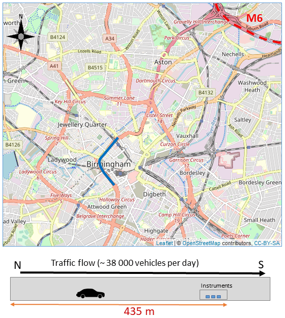
Figure 2Map of Birmingham City Centre showing the M6 motorway (red dashed line) and schematic of the Queensway Tunnel (highlighted in blue on the map). © OpenStreetMap contributors 2019. Distributed under a Creative Commons BY-SA License.
2.2 Fleet information
Data from an Automatic Number Plate Recognition (ANPR) camera commissioned by Birmingham City Council were used to obtain information on the vehicle fleet passing through the tunnel. ANPR data were taken from 8 to 11 November 2016 and included vehicle type, European emissions standard and capture rate of the vehicle number plates, on a 15 min timescale. The ANPR capture rate is based on a comparison of manual classified counts (MCC) with the ANPR data. The capture rate was typically around 90 % of MCC, with counts missing from ANPR usually as a result of the number plate being obscured (Rhead et al., 2012). We assumed the same fleet proportions for the missing vehicle counts and adjusted the final data accordingly. Figure 3 shows the mean hourly number of vehicles travelling through the tunnel during the weekdays and a breakdown of vehicles by type. The ANPR data were also compared to manual traffic counts performed at the exit of the southbound tunnel on selected days during the measurement period with good agreement. Approximately 37 700 vehicles travel through the southbound bore of the Queensway tunnel during an average weekday. The majority of these vehicles are petrol (40 %) and diesel (44 %) fuelled passenger cars, with the remaining fleet comprised primarily of diesel-fuelled light-goods vehicles (LGVs, e.g. vans, small pick-ups) (10.4 %), ordinary goods vehicles (OGVs, e.g. trucks, articulated vehicles) (2.5 %) and passenger vehicles (taxis and buses) (1.3 %).
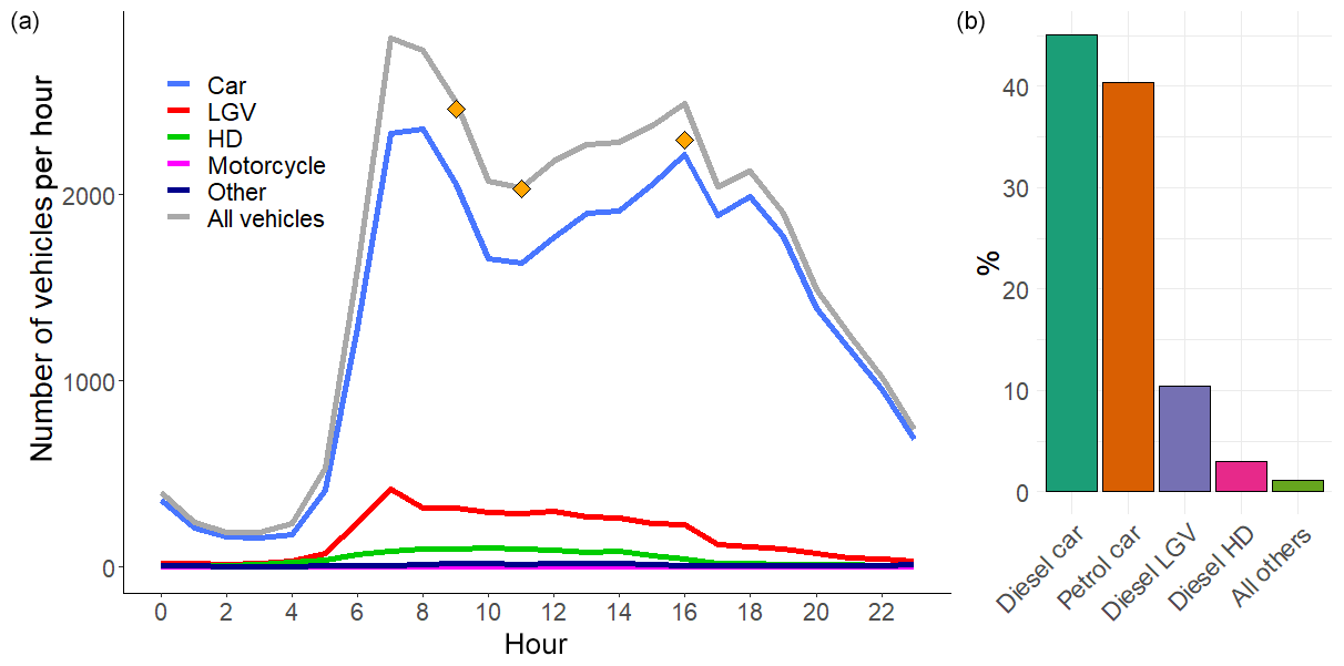
Figure 3(a) Average hourly vehicle fleet in the southbound tunnel from the corrected ANPR counts for weekdays (LGV = light goods vehicles, HD = heavy-duty vehicles, e.g. trucks, lorries and buses). Orange points represent the counts estimated from video footage recorded during the measurement period. (b) Percentage of vehicle types, determined from all weekday ANPR data in November 2016.
2.3 Instrumental techniques
The instruments were installed in the tunnel in close proximity (1.5 m) to the roadside and made measurements from 29 July until 8 August 2016. Access to the instruments was only possible when the tunnel was closed to traffic during maintenance periods, which occurred approximately every 2 weeks. Table 1 provides an overview of the instrumentation deployed in the tunnel during the campaign.
Table 1Overview of instruments deployed in the Queensway Tunnel.

Direct spectroscopic measurements of HONO and NO2 were made by broadband cavity enhanced absorption spectroscopy (BBCEAS) (Langridge et al., 2009; Thalman et al., 2015). The BBCEAS instrument operated in the wavelength range 363 to 388 nm, which includes a highly structured part of the NO2 spectrum and two HONO absorption bands at 368 and 385 nm. Ultraviolet light from an LED light source (LEDengin LZ1-10UV00, nominal peak wavelength = 365 nm) was directed through a cavity formed by two highly reflective mirrors (Layertec GmbH, 25 mm diameter, 0.5 m radius of curvature, high reflectivity 370 to 395 nm) separated by 80 cm, giving an effective path length of approximately 1.4 km. The mirrors were housed in bespoke mirror mounts (length = 11 cm) which were purged with nitrogen (0.9 L min−1 divided between the two mounts), and thus BBCEAS data were corrected for the cavity's length factor (LF = 1.37). The cavity was operated “open path”; i.e. the portion of the cavity between the mirror mounts was open to the ambient atmosphere. This open-path configuration has the advantage that there were no wall losses or heterogeneous production of HONO within the instrument. A Teflon tube was inserted between the mirror mounts in order to measure the reference spectrum of light transmitted when the cavity was purged with nitrogen. The reflectivity of the cavity mirrors (as a function of wavelength) was characterized in the laboratory before the campaign; their measured reflectivity peaked at 99.940 % at 387 nm. The reflectivity was verified in the field by measuring the 380 nm absorption band of O4 when purging the cavity with pure oxygen, and measurements taken at the start and end of the campaign agreed to within 4.5 %.
BBCEAS spectra were integrated for 20 s (the average of two 10 s acquisitions) using an OceanOptics QEPro spectrometer (instrument line shape = 0.20 nm HWHM). Spectra were fitted with reference absorption cross sections for HONO (Stutz et al., 2000), NO2 (Vandaele et al., 1998) and O4 (Hermans as given in the HITRAN database, Richard et al., 2012), and any remaining unfitted broadband absorption was attributed to extinction by ambient aerosol particles. Typical statistical errors for retrieving HONO and NO2 concentrations from the spectral structure were ±0.8 and ±0.9 ppbv, (1σ in 20 s) respectively. The BBCEAS measurements are also affected by systematic uncertainties in the molecules' reference absorption cross sections (typically ±3 %) and for determining the mirror reflectivity in the field (±4.5 %). Extinction by ambient aerosol also reduced the effective path length of the BBCEAS measurement. HONO retrievals tended to be dominated by statistical (spectral fitting) errors, whereas retrievals of the much higher ambient NO2 concentrations were dominated by the systematic uncertainties in the cross sections and the mirror reflectivity. For the mean HONO (3 ppbv) and NO2 (75 ppbv) amounts recorded during the campaign, the total measurement uncertainties (from combining the statistical and systematic errors) were ±1.2 ppbv for HONO and ±5 ppbv for NO2.
NO was measured by a commercial chemiluminescence NOx analyser (Thermo Environmental Instruments Inc: Model 42C). The detection limit of the 42C was determined from 3 times the standard deviation of the measurement in zero air and was calculated to be approximately 0.2 pbbv for a 1 min averaging period. The uncertainty of the instrument was estimated to be ±10 % from calibrations. The analyser is capable of measuring NO2 and NOx. However, the instrument utilizes a molybdenum converter to covert NO2 to NO, an approach which is known to be influenced by positive interference from other NOy species such as HONO, nitric acid (HNO3), peroxyacetyl nitrate (PAN) and alkyl nitrates (e.g. Dunlea et al., 2007; Villena et al., 2012); therefore the final NOx used in this study is calculated from the sum of the NO measured by the 42C and NO2 by the BBCEAS. The inlet for the 42C instrument was shared with a non-dispersive infrared instrument (LI-COR: Model LI-820) to measure CO2. The LI-COR was calibrated with pure N2 (0 ppmv CO2) and 1500 ppmv CO2 to determine the relative uncertainty (±5 %) and precision (1.2 %, 2σ). The LI-COR and 42C analysers were evaluated for drift from zero measurements taken before and after the measurement campaign. The drift for CO2 and NOx were determined to be 1.45 ppmv and 0.42 ppbv, respectively. The drift for both instruments was less than 2 % of the minimum measured values in the tunnel (NO = 1.27 %, CO2 = 0.35 %), and therefore no correction was deemed necessary here. A mini-meteorological station anemometer (Kestrel 4500) was deployed near the top of the tunnel (3 m above ground level and 1 m from the roadside) to measure the temperature, relative humidity and air flow in the tunnel.
3.1 Data overview
Figure 4 presents 15 min averaged time series for gases measured in the tunnel. NO, NO2, HONO and CO2 follow the same diurnal cycle as each other, indicating that they have a similar source. There is a clear difference in weekday and weekend diurnal cycles, with peaks associated with rush hour traffic observed in NO, NO2, HONO and CO2 during the weekdays, which are not present at the weekend. The measured concentrations are also lower at the weekend, on average. On weekdays, the mixing ratios of all gas species increase from around 06:00 (start of morning rush hour) and drop away in the afternoon. A large spike in the evening around 17:30 to 18:00 is observed, which coincides with congestion in the southbound tunnel during peak evening rush hour. The congestion is also evident in the lower mean vehicle speeds at 17:00 to 18:00 (Fig. S2).
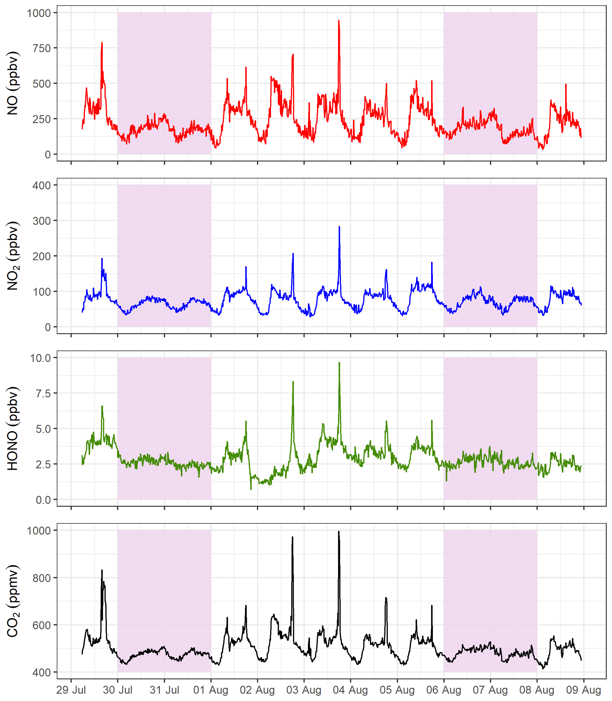
Figure 4The 15 min averaged measurements of NO, NO2, HONO and CO2 from the Queensway Tunnel between 29 July and 8 August 2016. Shaded areas indicate the weekends. Spikes in the measured mixing ratios on weekdays are the result of traffic congestion during morning and evening rush hour periods.
The mean weekday HONO mixing ratio during the day-time (06:00 to 19:59, calculated from the 15 min averages) is 3.4±1.0 ppbv (1σ), which decreased to 2.4±0.7 ppbv overnight. The maximum observed 15 min average HONO level occurred during the evening rush hour, reaching 9.7 ppbv on 3 August. Observed HONO levels in the current work are typically lower than in previous tunnel studies. Liang et al. (2017) measured a mean HONO level of 15.7±4.2 ppbv during their study in Hong Kong, whereas Kurtenbach et al. (2001) observed peak HONO levels of 45 ppbv in the day-time. Kirchstetter et al. (1999) only performed measurements between 16:00 and 18:00 in the Caldecott Tunnel, California, and observed a mean HONO level of 6.9±1.4 ppbv, higher than the mean level of 4.1±1.4 ppbv for the same hours in this study. The lower levels measured in the current study may be the result of differences in vehicle fleet between studies as discussed further in Sect. 3.3, in combination with shorter tunnel length (Table 2) and shorter distance of our sampling point into the tunnel.
Table 2Comparison of HONO∕NOx ratios from different tunnel studies.
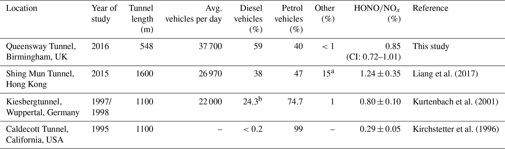
a LPG fuelled. b Includes LGVs and OGVs (assumption made here that these are diesel fuelled).
The persistence of HONO overnight is unlikely to be due to vehicle exhaust emissions, as traffic flow is low during this period, but is rather from background ambient HONO entering at the tunnel's entrance and from the heterogeneous formation of HONO on particles deposited onto the walls of the tunnel (Kurtenbach et al., 2001). This also suggests that vehicles were not the only source of HONO during the day, and the impact of heterogeneous HONO formation is considered in emission ratio calculations in Sect. 3.2.1.
From late evening on 1 August until mid-morning on 2 August the HONO mixing ratios are lower than otherwise observed for a weekday. Precipitation data from a nearby weather station (Fig. S3) revealed that it rained continuously from 17:00 on 1 August to 16:00 on 2 August with corresponding high relative humidity recorded inside the tunnel. It is likely that wet surfaces inside the tunnel, as a result of spray from tyres, resulted in a loss of HONO. The Henry's law constant (in water) of HONO ( mol m−3 Pa−1) is approximately 4800 times greater than that of NO2 ( mol m−3 Pa−1) (Sander, 2015), and therefore HONO is likely to be washed out more rapidly than NO2 on wet surfaces, resulting in a reduction in the HONO∕NOx ratios. As a result, this precipitation event was excluded from the final dataset for calculation of emission ratios.
3.2 Relative HONO emission ratios
To determine a HONO∕NOx emission ratio representative of direct exhaust emissions, corrections for both heterogeneous formation of HONO from NO2 and background HONO levels were considered.
3.2.1 Heterogeneous HONO formation from NO2
A number of heterogeneous reactions resulting in the formation of HONO have been proposed in the literature; however, the formation of HONO from NO2 on humid surfaces (Reaction R3) is thought to be the main pathway (Spataro and Ianniello, 2014 and references therein).
The rate coefficient for Reaction (R3) (khet) is dependent on the geometric uptake coefficient of NO2 on the tunnel walls (γgeo) and is given by
where is the mean molecular velocity of NO2 and S∕V is the surface-to-volume ratio of the tunnel (Kurtenbach et al., 2001). Kurtenbach et al. (2001) performed laboratory experiments to measure HONO generated on tunnel wall residue to directly calculate γgeo and determined min−1.
The rate of formation of HONO from NO2 can then be calculated via Eq. (2).
where dt is the residence time of the gases in the tunnel from the entrance to the sampling point.
Kurtenbach et al. (2001) calculated that the heterogeneous conversion on the tunnel wall contributed to approximately 13 % of the measured HONO during the day and up to 80 % at night (for a maximum NO2 mixing ratio of 250 ppbv). This result is in contrast to measurements obtained in the Caldecott Tunnel by Kirchstetter et al. (1996), who showed that the HONO∕NOx ratio did not change between the middle of the tunnel and the tunnel exit, suggesting that there was no significant formation of HONO (or deposition of HONO) on the tunnel walls in their study.
Liang et al. (2017) determined min−1 in the Shing Mun Tunnel, Hong Kong, from using an upper limit of as calculated by Kurtenbach et al. (2001). Using wind speed data in the tunnel to determine the residence time, Liang et al. (2017) found that the contribution of HONO∕NOx from heterogeneous reactions on the tunnel walls alone was 0.04 % on average. Since this value was less than the error when calculating HONO∕NOx from direct emissions, the authors did not perform any corrections to their final HONO∕NOx ratio. As there is no consensus in the literature about the relative contribution from tunnel walls to measured HONO, we calculated the contribution from heterogeneous HONO formation in the Queensway tunnel during the measurement period. Using Eq. (1), a geometric uptake coefficient for NO2 of and the surface-to-volume ratio of the Queensway tunnel (0.64 m−1), we calculated khet to be min−1.
The Kestrel anemometer used in this study logged data every 20 min, and as a result, the wind speed measurements inside the tunnel only provide a “snap-shot” of the data and are dependent on the traffic flow. Care should be taken when using wind speed measured by an anemometer to calculate the air residence time in a tunnel. Rogak et al. (1998) compared residence times in a tunnel calculated using an SF6 tracer and anemometer data and found that the wind speed in the tunnel measured by the anemometer overestimates volumetric flow during high wind speeds and underestimates when wind speed is low, requiring a correction factor for the determination of emission factors in the tunnel. Tracer measurements were not performed during our study, and consequently a modelling approach was used to correct the wind speed data from the anemometer. As outlined below, the wall source contribution to the observed HONO was small (∼5 % on average) during the day-time periods used to derive our final results.
“True” wind speeds were inferred from computational fluid dynamics (CFD) modelling of CO2 profiles measured along the tunnel. After the campaign, the LI-COR CO2 instrument was installed in a van and driven repeatedly through the southbound bore of the tunnel at four different times of the day (late morning, late afternoon, evening and at night). Data recorded when the van was inside the tunnel were extracted from the CO2 time series. The timestamps of these data points were converted into distance along the tunnel using the speed of the van and the time that it entered the tunnel, as recorded by a camera mounted on the van's dashboard. The CO2 data were then averaged into 50 m bins along the tunnel to produce a profile of the CO2 concentration increasing with distance into the tunnel. The CO2 profiles were simulated by a CFD model which took as its inputs the tunnel's physical dimensions, the anemometer wind speed, the ANPR traffic counts and traffic composition, and emission factors from the DEFRA Emissions Factor Toolkit version (EFT v8.0.1) (DEFRA, 2017). Further information on the DEFRA EFT is provided in the supplementary material. The wind speeds that produced the optimum fits between modelled and measured CO2 profiles are shown as the crosses in Fig. S4. These wind speeds match closely with the anemometer wind speeds increased by a factor of 3.0 and they correctly capture the day- and night-time differences. The optimum CFD-inferred wind speeds at 10:00, 16:00 and 20:00 (3.4 to 3.9 m s−1) are also in agreement with the 3.6 m s−1 wind speed (06:00 to 23:59) in the tunnel study by Liang et al. (2017) and are consistent with the empirical correction factor produced by Rogak et al. (1998) of ×3.5 for an anemometer-measured wind speed of 1.5 m s−1, applicable during much of the day-time. The results of CFD modelling of CO2, NO2 and HONO profiles measured in the Queensway tunnel will be published in a separate paper.
During the night, the measured wind speed was often below the minimum speed required to turn the anemometer's impeller (<0.4 m s−1) so the residence time of the air parcel overnight is difficult to determine directly. As a result, we focus here on the heterogeneous formation of HONO in the tunnel during the day-time (see comments below, in Sect. 3.2.3, regarding use of day-time-only data to infer the fleet average emission ratios). Between 06:00 and 19:59 the mean wind speed in the tunnel was 3.9 m s−1, giving a residence time of air in the tunnel up to the sampling point of 1.86 min. If we assume the mean residence time of NO2 emissions in the tunnel is half of this residence time (Liang et al., 2017; Pierson et al., 1978), the HONO produced from heterogeneous formation on the tunnel walls is 0.18 ppbv for a mean daily weekday NO2 mixing ratio of 98 ppbv, which is approximately 5 % of the mean measured HONO during the day. Although the mean heterogeneous contribution to HONO during the day-time is small, the heterogeneous contribution is higher (8 %) when the tunnel becomes congested and the residence time of the air in the tunnel increases. Therefore, the final HONO data used in this study were corrected for the heterogeneous HONO contribution using measured NO2 and the modelled wind speed, to better represent the direct HONO emissions in the tunnel.
3.2.2 Background corrections for HONO, NOx and CO2
As vehicles travel through the tunnel, cleaner air from outside is drawn into the tunnel, which dilutes the vehicle emissions in a process known as the piston effect. To obtain direct vehicle emission measurements it is necessary to correct for this dilution by subtracting ambient background levels from the concentrations measured inside the tunnel. As no concurrent measurements were available at the tunnel entrance during this campaign, ambient NOx, HONO and CO2 data from nearby air monitoring stations were used to correct for the background levels. Hourly averaged background NOx mixing ratios during the measurement period were taken from Acocks Green (AG), an Automatic Urban Rural Network (AURN) site located 6.9 km south-east of the Queensway Tunnel (http://uk-air. defra.gov.uk/, last access: 26 January 2020). The AURN station does not measure HONO or CO2, so data previously taken at the Birmingham Air Quality Supersite (BAQS) on the University of Birmingham campus (52∘27′1′′ N, 1∘55′30′′ W) 3 km south-west of the tunnel were used in this study. As CO2 is well mixed within the troposphere, variability in background CO2 mixing ratios is primarily the result of a changing boundary layer height. Therefore, in this study, an average diurnal CO2 cycle measured at BAQS was used to correct for background CO2. The overnight background corrected CO2 () levels dropped to near zero (see Fig. 5c), suggesting that the procedure was suitable. HONO on the other hand has a much shorter lifetime than CO2, and HONO mixing ratios vary depending on local sources and the availability of NO2 (Crilley et al., 2016). An average diurnal HONO∕NOx cycle (Fig. S5) was calculated from measurements taken at BAQS between 18 March and 1 April 2015 (Singh, 2017) and applied to the background NOx from Acocks Green to determine hourly background HONO mixing ratios (Eq. 3).
Figure 5 shows the hourly time series of NOx, HONO and CO2 measured in the tunnel and the corresponding data corrected for background mixing ratios. The results show that mixing ratios measured in the tunnel were, on average, 73 and 44 times higher than the background NOx and HONO, respectively, suggesting that direct emissions from vehicles were indeed the dominant source of these gases. Consequently, any uncertainties in the background HONO mixing ratios that were subtracted from the measured HONO have little impact on the final results. In the following sections, the final HONO dataset (ΔHONO) is corrected for both background HONO levels and the heterogeneous HONO contribution.
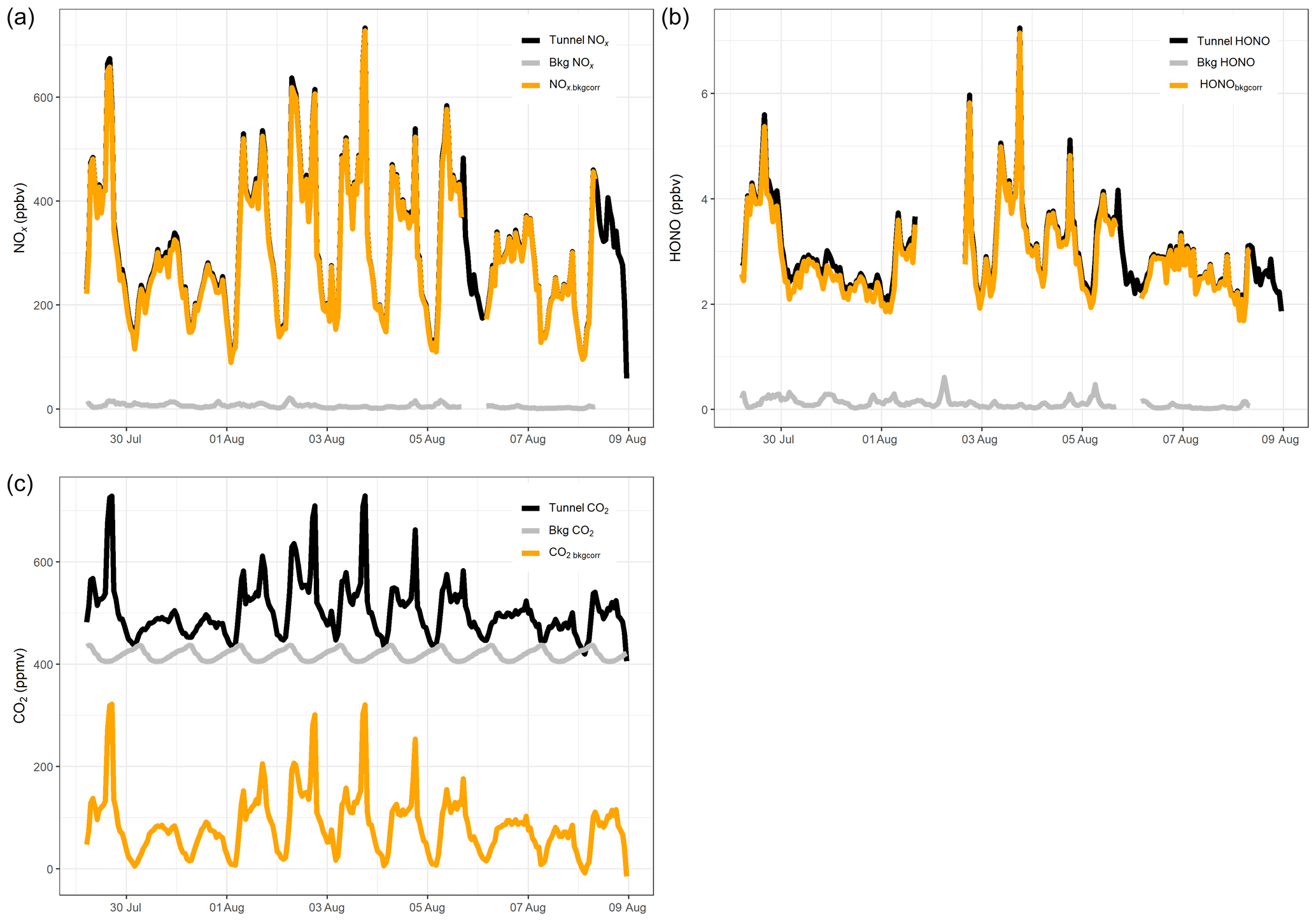
Figure 5Hourly averaged time series (a) NOx in the tunnel and from Acocks Green urban background station. (b) HONO in the tunnel and estimated background HONO. (c) CO2 in the tunnel and background CO2 measured at BAQS.
3.2.3 HONO emission ratios
To determine the HONO to NOx emission ratio, a reduced-major-axis (RMA) regression (Fig. 6) was performed using the weekday hourly averaged data from 06:00 to 19:00, i.e. when there was minimal contribution from heterogeneous HONO sources and the traffic flow was high (>1500 vehicles per hour). The slope of the regression gives an average emission ratio of % (95 % confidence interval = 0.72 % to 1.01 %) for this time period.
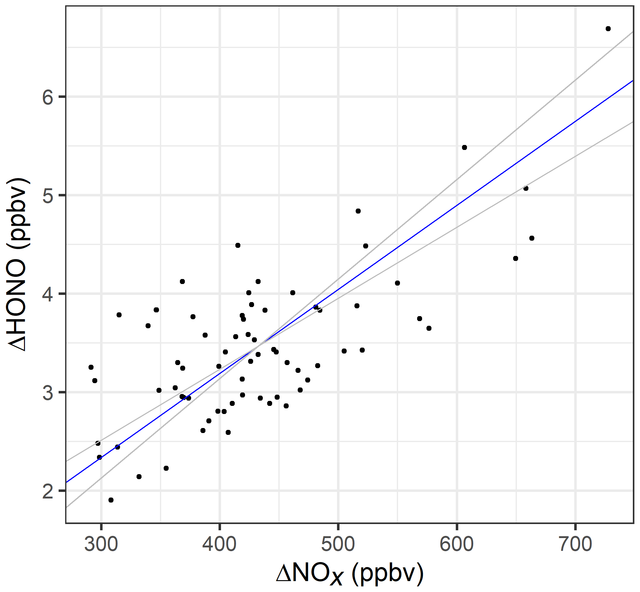
Figure 6RMA regression for hourly averaged ΔNOx versus ΔHONO, for weekdays between 06:00 and 19:00. The blue line represents the RMA slope and the grey lines the 95 % confidence intervals of the regression.
Figure 7a shows that the ΔHONO∕ΔNOx emission ratio varies during the day, from 0.66 % at 07:00 to 1.10 % at 19:00. In this section, we explore the relationship between ΔHONO∕ΔNOx and changes in vehicle fleet composition using information on fuel and vehicle types from the ANPR dataset. Figure 7c shows the fraction of diesel and non-diesel (petrol, LPG and electric) vehicles travelling through the Queensway tunnel during an average weekday. Between 06:00 and 17:00, the ΔHONO∕ΔNOx ratio appears to vary closely with changes in the fraction of diesel vehicles, with both variables peaking at 10:00 when the ΔHONO∕ΔNOx emission ratio reaches a value of 0.91 % and the percentage of diesel-fuelled vehicles in the fleet reaches a maximum of 66 %.
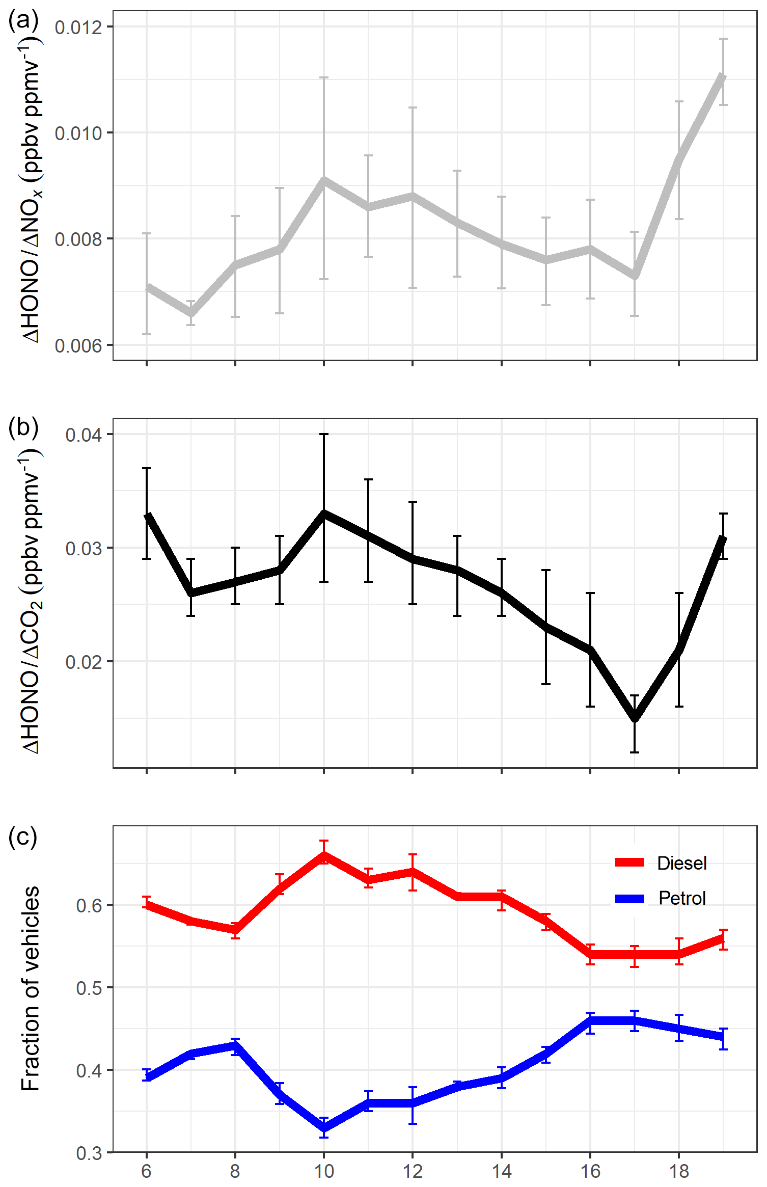
Figure 7(a) Hourly averaged ΔHONO∕ΔNOx, (b) hourly averaged ΔHONO∕ΔCO2, and (c) fraction of diesel and non-diesel (petrol, biofuel, electric) vehicles calculated from the total petrol and diesel vehicles, for the period between 06:00 and 19:00 during weekdays. Error bars represent 1σ standard deviation of the mean across the different days of this study.
The ΔHONO∕ΔCO2 ratio (Fig. 7b and Table S2) also follows the change in fleet composition, with a higher ratio observed at 10:00 (3.3 %) compared to 17:00 (1.5 %). However, this may also be the result of higher CO2 emissions from petrol-fuelled vehicles compared to diesel vehicles; for example, a study of 149 passenger cars showed that CO2 emissions were 13 % to 66 % higher for petrol vehicles than diesel (O'Driscoll et al., 2018). Modelled emission factors from the DEFRA Emissions Factors Toolkit (EFT v8.0.1) indicate a maximum in the CO2 emissions (mg per vehicle per kilometre) at 17:00 (Fig. S6), in line with the 46 % maximum in the non-diesel vehicle fraction at evening rush hour.
From 17:00 to 19:00 the relationship between the ΔHONO ratios and fuel type is less clear. During this period the fraction of diesel vehicles remains almost constant; however, the ΔHONO∕ΔNOx and ΔHONO∕ΔCO2 emission ratios both sharply increase. Analysis of the modelled NOx and CO2 emission factors from the EFT (Fig. S6) indicate a decrease in both NOx and CO2 emission factors from 17:00 to 19:00, which is likely to be related to the total vehicle flow and lower vehicle speed at times of peak congestion (because the fleet composition remains very similar). The EFT does not have the capability to determine a HONO emission factor, and therefore information on HONO emission variability with speed and vehicle flow is not available a priori. However, assuming the HONO emissions do not reduce by the same percentage after 17:00, this would lead to the increase in the observed ΔHONO∕ΔNOx and ΔHONO∕ΔCO2 ratios. As no conclusion can be made at this point, without additional information, we focus the analysis in the following section on the data between 06:00 and 17:00 only.
Ho et al. (2007) used Eq. (4) to determine emission factors (mg per vehicle per kilometre) for diesel- and non-diesel-fuelled vehicles based on a method described by Pierson et al. (1996).
where x is the fraction of diesel-fuelled vehicles, EFDV is the emission factor for diesel vehicles, EFNDV is the emission factor for non-diesel vehicles and EF is the emission factor for the mixed fleet. In this format, a linear regression of x versus EF, based on Eq. (4), gives EFDV at x=1 and EFNDV at x=0.
In this study, instead of calculating emission factors, we investigated the applicability of Eq. (4) to determine ΔHONO∕ΔNOx emission ratios for diesel (ERDV) and non-diesel (ERNDV) vehicles (see Fig. S7). Extrapolating the best-fit line in Fig. S7 to x=1 gives a plausible emission ratio for diesel vehicles of ER %. Unfortunately, this method resulted in an unrealistically small negative emission ratio for non-diesel vehicles (ER %). This method may not be appropriate for the current work because the range in the fuel fraction of vehicles is small, and thus extrapolating to x=0 and x=1 resulted in large uncertainties.
An alternative approach is to determine emission ratios using a pair of simultaneous equations based on the fraction of diesel vehicles and ΔHONO∕ΔNOx values for different hours of the day. For example, using the data as given in Table S2, the equation at 17:00 is given by
Using another equation for a different hour (i.e. different set of fractions), the values for ERDV and ERNDV can be determined. Care must be taken when interpreting these results, however, as the calculated ERs depend on the selection of pairs of measurement points and some pairs from our data resulted in negative ER values. Thus average ERs were determined using many pairs of simultaneous equations. Here we calculated the average of 10 ERs, using one set of fractions at 17:00 and a second set for each hour from 06:00 to 15:00. The data from 16:00 were not used here as there was no change in the diesel fraction between 16:00 and 17:00. The means (±1σ) for ERDV and ERNDV are 1.04±0.47 % and 0.37±0.55 %, respectively, suggesting that diesel-fuelled vehicles do have higher ΔHONO∕ΔNOx ratios.
It has previously been suggested that higher HONO∕NOx ratios are observed when the tunnel fleet contains a greater number of heavy-duty vehicles (Trinh et al., 2017). A similar calculation to that outlined in the previous paragraph was performed here to determine the average emission ratio for cars and for heavy-duty vehicles (goods vehicles and buses) by apportioning the observed ΔHONO∕ΔNOx ratios between the car and heavy-duty vehicle numbers given in Table S2. The ΔHONO∕ΔNOx emission ratio for heavy-duty vehicles (ERHD) is estimated to be 1.3±0.63 %, approximately 1.9 times higher than the ratio determined for cars (ER %). The impact of heavy-duty vehicles on the HONO∕NOx emission ratio is discussed further in Sect. 3.3.
It should be noted that the methods described above can only provide an estimate of the emission ratios for different fuel and vehicle types. In our study, the variability in the fraction of diesel vehicles and heavy-duty vehicles across the day was small, and therefore extracting emission ratios for individual vehicle types is challenging. To obtain more precise emission ratios for different engine types, a larger dataset (i.e. longer time series) and fully contemporaneous ANPR data would be required.
3.3 Comparison of HONO∕NOx emission ratios across tunnel studies
Table 2 shows a comparison of measured HONO∕NOx emission ratios from studies performed in road tunnels, along with summaries of their reported vehicle fleets. The lowest HONO∕NOx ratio (0.29 %) was measured in the Caldecott tunnel, California (Kirchstetter et al., 1996). As 99 % of the fleet was comprised of petrol-fuelled vehicles, the low HONO∕NOx ratio is expected because the analysis in Sect. 3.2.3 above and previous dynamometer studies have both demonstrated that petrol vehicles typically emit less HONO than diesel vehicles. On the other hand, Liang et al. (2017) observed a HONO∕NOx emission ratio of 1.24±0.35 % in the Shing Mun Tunnel, Hong Kong, in 2015, approximately 1.4 times higher than in the current work despite the Queensway Tunnel having a higher proportion of diesel vehicles compared to the Shing Mun Tunnel (59 % and 38 % respectively). The differences observed in the HONO∕NOx emission ratio between the Shing Mun and Queensway tunnel studies may therefore be related to (1) the percentage of heavy-duty and goods vehicles within the fleet, and (2) exhaust after-treatment technologies that affect NO2 emitted directly from vehicle exhausts (known as primary NO2).
In addition to these two points, which are discussed further below, it should also be noted that the fleet in the Shing Mun Tunnel consisted of 15 % vehicles fuelled by liquefied petroleum gas (LPG). On-road sampling of emissions from buses fuelled by diesel and LPG in Hong Kong have indicated that LPG vehicles have lower NOx emissions when compared to diesel vehicles (Ning et al., 2012). However, as far as we are aware there have been no published studies investigating HONO emissions from LPG-fuelled vehicles, and therefore no conclusions can be made at this point regarding the impact of the LPG fleet on the observed differences in HONO∕NOx ratios.
Liang et al. (2017) investigated the impact of diesel particle filters (DPFs) on HONO vehicle emissions and found that HONO emissions ratios were higher in vehicles equipped with DPFs (based on a higher ΔNO2∕ΔNOx ratio) and suggest that this may be due to HONO formation from heterogeneous reactions involving NO2 and black carbon within the filter. The diesel oxidation catalysts (DOCs) oxidize hydrocarbons and CO in excess oxygen over platinum–palladium catalysts; however, NO can also be oxidized to NO2 during this process. DPFs were mandatory for all new diesel vehicles from 2009 (Euro class V) and operate by trapping soot in the exhaust where it is then oxidized at high temperatures. To ensure the filters do not become blocked from engines that run at lower temperatures, many DPFs use catalysts to convert NO to NO2 to periodically oxidize the soot (He et al., 2015; Kim et al., 2010). Consequently, DOCs and DPFs both result in an increase in NO2 emitted from exhausts, which may also lead to an increase in HONO emissions.
Liang et al. (2017) estimated that half of the diesel fleet in their study were buses and goods vehicles (Euro class IV and above) equipped with diesel particulate filters. In the current work less than a quarter of diesel-fuelled vehicles were goods vehicles or buses, and of those only 58 % were Euro class V and above (i.e. with DPFs fitted). As a result, the percentage of diesel vehicles emitting high NOx and HONO levels is expected to be much lower in the Queensway tunnel than the Shing Mun Tunnel, and this likely accounts for the lower HONO∕NOx emission ratio we observed. In contrast, in the Kiesbergtunnel (Kurtenbach et al., 2001), medium and heavy-duty vehicles represented 12 % of the fleet (6 % heavy-duty trucks, 6 % commercial vans), similar to the fleet in the Queensway tunnel, which may explain why the observed HONO∕NOx emission ratios were so similar (0.85 % and 0.8 %, for the Queensway tunnel and Kiesbergtunnel studies, respectively). It should be noted that the Kiesbergtunnel study was done before the Euro III standard came into effect, so higher emissions of NOx are expected compared to higher Euro standard vehicle classes. However, few of these vehicles in the Kiesbergtunnel would have been fitted with DOCs or DPFs, so this may have offset the amount of NO2 (and thus HONO) emitted.
Recent trend analysis studies have shown that primary NO2 has been decreasing over the last decade in the UK (Carslaw et al., 2016; Matthaios et al., 2019) and across Europe (Grange et al., 2017). For example, the mean NO2∕NOx emission ratio measured from ambient roadside monitoring sites in inner London has decreased from a peak value of 25 % in 2009 to 15 % in 2014 (Carslaw et al., 2016). Although the exact cause of the NO2 reduction is not clear, it is thought that the introduction of after-treatment technologies, such as selective catalytic reduction (SCR) installed on buses and heavy-duty vehicles, and a reduction in the use of platinum group metals in catalysts may have contributed to the observed decrease (Carslaw et al., 2016; Grange et al., 2017). With a reduction in NO2 emissions from diesel vehicles overall, a decrease in HONO may also be expected in the UK. In contrast, Wang et al. (2018) reported an increase in the NO2∕NOx ratio at the outlet of the Shing Mun Tunnel, from 9.5 % in 2003 to 16.3 % in 2015. Therefore, the higher HONO∕NOx ratio observed in Hong Kong (Liang et al., 2017) compared to our current work may also be related to differences in primary NO2 emissions. It should be noted that in the study by Wang et al. (2018), NO2 was measured using a standard chemiluminescence monitor, which typically use a molybdenum converter. Molybdenum converters also convert other NOy species, such as HONO, resulting in an overestimation of the reported NO2. However, as the HONO∕NOx ratio was only 1.24 %, it is unlikely that HONO has contributed to the factor of 1.7 increase in primary NO2 recorded near the Shin Mung Tunnel.
Previous work has shown that ambient HONO has high heterogeneity when sampled close to roads (Crilley et al., 2016). Here we use the mean HONO∕NOx emission factor of 0.85 %, determined from the tunnel measurements in Sect. 3.2.3, to investigate the contribution of direct HONO vehicle emissions to ambient HONO levels in urban and suburban areas. Measurements of HONO and NOx were taken in a mobile laboratory on a return journey between Birmingham and Leicester, two cities in the UK Midlands separated by 55 km (straight line measurement from city centres). NO and NO2 were measured every 60 s by our chemiluminescence analyser fitted with a molybdenum NO2 converter (Thermo 42i-TL). As discussed in Sect. 2.3, molybdenum converters are known to result in interferences from NOy species, and therefore the NOx measurements presented here represent an upper limit on NO+NO2 concentrations. HONO was measured every 5 min with a Long-Path Absorption Photometer (LOPAP, Model 03, QUMA). Measurement uncertainties are primarily the result of uncertainties in the calibrations and are estimated to be 5 % and 10 %, for NOx and HONO, respectively. Further details regarding the measurement techniques and the driving route can be found in Crilley et al. (2016).
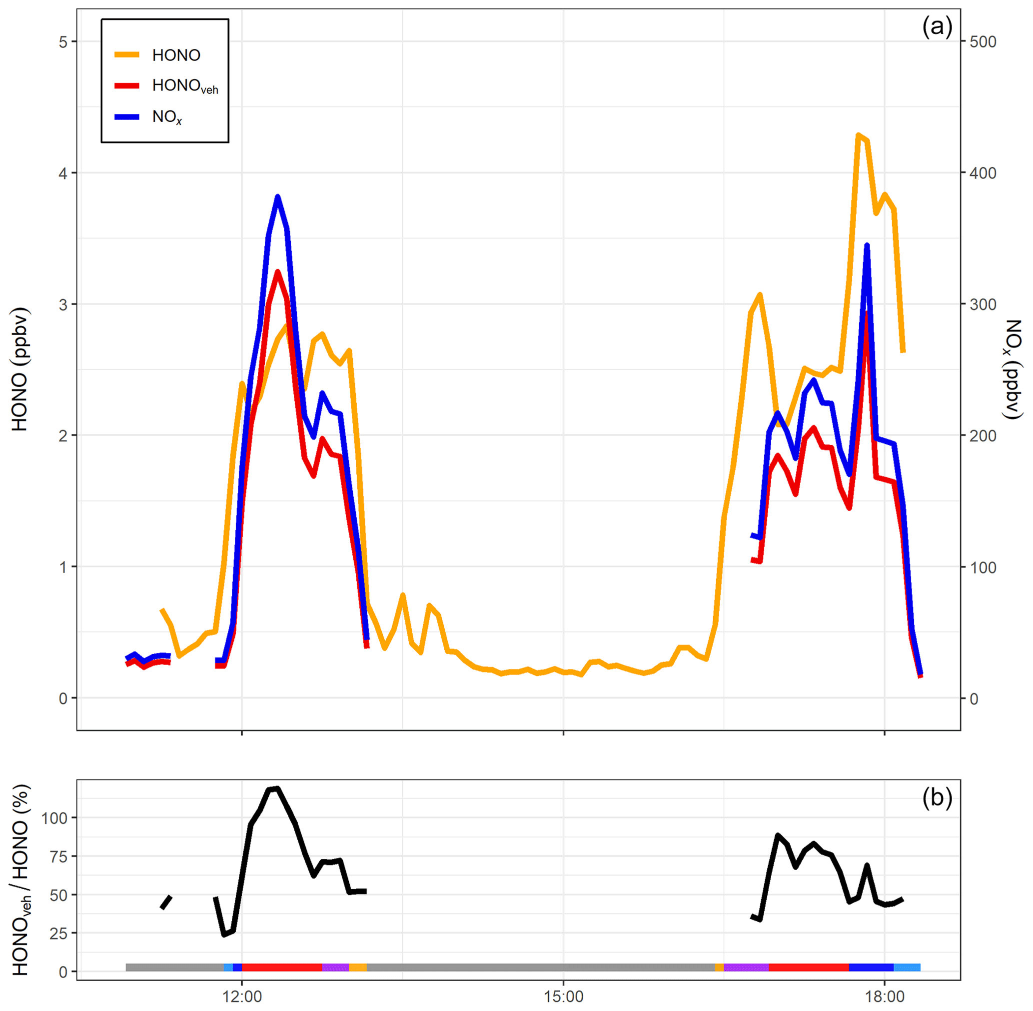
Figure 8(a) NOx, HONO and inferred vehicle exhaust HONO from mobile measurements taken on 23 October 2015 along a return journey between Birmingham and Leicester (Crilley et al., 2016). (b) Ratio of vehicle-produced HONOveh to measured HONO (%) for the same period. Grey shaded areas represent non-driving periods, i.e. when the mobile laboratory was parked either at the University of Birmingham or University of Leicester campus. Other colours represent measurements around the University of Birmingham campus (light blue), the A38 road through Birmingham city centre (dark blue), M6 and M69 motorways (red), Leicester Ring Road (purple) and measurements around the University of Leicester campus (orange). HONOveh∕HONO ratios above 100 % are the result of uncertainties in the HONO and NOx measurements and the HONO∕NOx emission ratio.
Figure 8 shows HONO and NOx mixing ratios measured during the transect from Birmingham to Leicester and the return journey on 23 October 2015. Also shown is the directly emitted vehicular HONO (HONOveh) calculated from the mean ΔHONO∕ΔNOx emission ratio (0.85 %). For the two transects, HONOveh contributed on average 66 % to the total measured HONO. The highest contribution was observed on the M6 motorway, where HONOveh typically accounted for 86 % of the measured HONO. During the motorway segments of the journeys, the mobile laboratory was operating in “chase mode”, i.e. deliberately sampling plumes from a single vehicle ahead. Therefore, it was likely the high HONOveh∕HONO ratios observed on the motorway were the result of predominantly sampling vehicle emission plumes with low background contribution. The lowest HONOveh contribution was observed around the Birmingham University campus (24 %), which is expected as traffic density was low in this area. Whilst travelling through Birmingham city centre, HONOveh∕HONO increased to 70 %, indicating that vehicle exhaust emissions were the dominant source of HONO in this area. This value is higher than determined by Tong et al. (2016) in Beijing (48 %); however, in our study we were sampling directly on the road, whereas the site in Beijing was located in a building at the Institute of Chemistry, Chinese Academy of Sciences, and therefore significantly less influenced by direct traffic sources. This estimate neglects the differing atmospheric lifetimes of HONO and NOx; the longer lifetime of the latter implies that HONO∕NOx ratios will fall as the air mass ages. Accordingly, estimates of the vehicular contribution derived from measurements made as close as possible to the emission source, i.e. on the roadway, as described here, will give the highest estimate of the relative importance of vehicle emissions.
Overall direct vehicle emissions can be an important source of HONO in urban areas, particularly near roads with high traffic density. Further investigation is required to quantify the impact of HONO emissions in these areas on the chemistry of the overlying atmosphere.
Measurements of HONO, NOx and CO2 were performed in a city centre road tunnel in Birmingham, UK, for 2 weeks in July and August 2016 to investigate direct HONO emissions from vehicle exhausts under real-world driving conditions. HONO mixing ratios peaked when NOx and CO2 peaked during traffic congestion in the weekday evening rush hour (17:30 to 18:00), confirming that vehicle exhausts were the dominant source of HONO in the tunnel.
A HONO∕NOx emission ratio of 0.85 % (0.72 % to 1.01 % at 95 % confidence interval) was determined for an average weekday fleet comprising 59 % diesel-fuelled vehicles. Our value is similar to the ratio of 0.8 % which is typically used in modelling studies and which was determined for a predominately petrol-fuelled fleet over 20 years ago in Germany. The results show that despite an increase in the proportion of diesel-fuelled vehicles over the past two decades in Europe, and updated emissions control technologies, the HONO∕NOx emission ratio has not varied significantly. A comparison with a tunnel study in Hong Kong suggested that the HONO∕NOx ratio may be less dependent on the percentage of diesel vehicles but rather the percentage of large goods vehicles within the fleet, and the after-treatment technologies implemented on those vehicles.
The HONO∕NOx emission ratio determined in this study was used to investigate the contribution of vehicle exhaust HONO to ambient HONO in Birmingham. The results show that direct vehicle emissions contribute up to 70 % of the total measured HONO in the city centre. As direct HONO emissions were found to be the dominant source where traffic density is high, it is important to obtain fuel-based emission ratios which also take into account after-treatment technologies, to ensure models can accurately simulate day-time OH radical production rates.
In this study the focus has been primarily on HONO emissions from diesel and petrol-fuelled vehicles. However, in countries where alternative fuels such as liquefied petroleum gas (LPG) and compressed natural gas (CNG) are becoming more prevalent, in particular in the public transport sector, further investigation into HONO emissions from these fuel types is needed.
Hourly averaged fuel type, vehicle type and emission ratios are available in the Supplement. The 15 min dataset from the tunnel measurements is available from the authors on request.
The supplement related to this article is available online at: https://doi.org/10.5194/acp-20-5231-2020-supplement.
The study was conceived by WJB, FDP and SMB. Measurements were performed by LJK, LRC, TJA, SMB and FDP. Formal analysis performed by LJK, TJA and SMB. LJK prepared the paper with contributions from all co-authors.
The authors declare that they have no conflict of interest.
The authors would like to thank the staff from Amey for their help in accessing the measurement site. We would also like to thank Birmingham City Council for their input and provision of ANPR data. This work was funded by the Natural Environment Research Council (NERC) project “Sources of Nitrous Acid in the Atmospheric Boundary Layer”.
This research has been supported by the Natural Environment Research Council (grant nos. NE/M013545/1 and NE/M010554/1).
This paper was edited by Andreas Hofzumahaus and reviewed by two anonymous referees.
Alicke, B., Platt, U., and Stutz, J.: Impact of nitrous acid photolysis on the total hydroxyl radical budget during the Limitation of Oxidant Production/Pianura Padana Produzione di Ozono study in Milan, J. Geophys. Res.-Atmos., 107, LOP 9-1–LOP 9-17, https://doi.org/10.1029/2000JD000075, 2002.
Ammann, M., Kalberer, M., Jost, D. T., Tobler, L., Rössler, E., Piguet, D., Gäggeler, H. W., and Baltensperger, U.: Heterogeneous production of nitrous acid on soot in polluted air masses, Nature, 395, 157–160, https://doi.org/10.1038/25965, 1998.
Arens, F., Gutzwiller, L., Baltensperger, U., Gäggeler, H. W., and Ammann, M.: Heterogeneous Reaction of NO2 Diesel Soot Particles, Environ. Sci. Technol., 35, 2191–2199, https://doi.org/10.1021/es000207s, 2001.
Aubin, D. G. and Abbatt, J. P. D.: Interaction of NO2 with hydrocarbon soot: Focus on HONO yield, surface modification, and mechanism, J. Phys. Chem. A, 111, 6263–6273, https://doi.org/10.1021/jp068884h, 2007.
Bohnenstengel, S. I., Belcher, S. E., Aiken, A., Allan, J. D., Allen, G., Bacak, A., Bannan, T. J., Barlow, J. F., Beddows, D. C. S., Bloss, W. J., Booth, A. M., Chemel, C., Coceal, O., Di Marco, C. F., Dubey, M. K., Faloon, K. H., Flemming, Z. L., Furger, M., Gietl, J. K., Graves, R. R., Green, D. C., Grimmond, C. S. B., Halios, C. H., Hamilton, J. F., Harrison, R. M., Heal, M. R., Heard, D. E., Helfter, C., Herndon, S. C., Holmes, R. E., Hopkins, J. R., Jones, A. M., Kelly, F. J., Kotthaus, S., Langford, B., Lee, J. D., Leigh, R. J., Lewis, A. C., Lidster, R. T., Lopez-Hilfiker, F. D., McQuaid, J. B., Mohr, C., Monks, P. S., Nemitz, E., Ng, N. L., Percival, C. J., Prévôt, A. S. H., Ricketts, H. M. A., Sokhi, R., Stone, D., Thornton, J. A., Tremper, A. H., Valach, A. C., Visser, S., Whalley, L. K., Williams, L. R., Xu, L., Young, D. E., and Zotter, P.: Meteorology, air quality, and health in London: The ClearfLo project, B. Am. Meteorol. Soc., 96, 779–804, https://doi.org/10.1175/BAMS-D-12-00245.1, 2015.
Calvert, J. G., Yarwood, G., and Dunker, A. M.: An evaluation of the mechanism of nitrous acid formation in the urban atmosphere, Res. Chem. Intermediat., 20, 463–502, https://doi.org/10.1163/156856794X00423, 1994.
Carslaw, D. C. and Ropkins, K.: openair – An R package for air quality data analysis, Environ. Modell. Softw., 27–28, 52–61, https://doi.org/10.1016/j.envsoft.2011.09.008, 2012.
Carslaw, D. C., Murrells, T. P., Andersson, J., and Keenan, M.: Have vehicle emissions of primary NO2 peaked?, Faraday Discuss., 189, 439–454, https://doi.org/10.1039/C5FD00162E, 2016.
Cheng, J., Karambelkar, B., and Xie, Y.: leaflet: Create Interactive Web Maps with the JavaScript “Leaflet” Library, R package version 2.0.3, available at: https://CRAN.R-project.org/package=leaflet (last access: 28 April 2020), 2019.
Crilley, L. R., Kramer, L., Pope, F. D., Whalley, L. K., Cryer, D. R., Heard, D. E., Lee, J. D., Reed, C., and Bloss, W. J.: On the interpretation of in situ HONO observations via photochemical steady state, Faraday Discuss., 189, 191–212, https://doi.org/10.1039/c5fd00224a, 2016.
DEFRA: Emission Factors Toolkit for Vehicle Emissions, available at: https://laqm.defra.gov.uk/review-and-assessment/tools/emissions-factors-toolkit.html (last access: 14 July 2019), 2017.
DfT: Vehicle licensing statistics: 2016, available at: https://www.gov.uk/government/statistics/vehicle-licensing-statistics-2016 (last access: 26 April 2019), 2017.
Dunlea, E. J., Herndon, S. C., Nelson, D. D., Volkamer, R. M., San Martini, F., Sheehy, P. M., Zahniser, M. S., Shorter, J. H., Wormhoudt, J. C., Lamb, B. K., Allwine, E. J., Gaffney, J. S., Marley, N. A., Grutter, M., Marquez, C., Blanco, S., Cardenas, B., Retama, A., Ramos Villegas, C. R., Kolb, C. E., Molina, L. T., and Molina, M. J.: Evaluation of nitrogen dioxide chemiluminescence monitors in a polluted urban environment, Atmos. Chem. Phys., 7, 2691–2704, https://doi.org/10.5194/acp-7-2691-2007, 2007.
Elshorbany, Y. F., Kurtenbach, R., Wiesen, P., Lissi, E., Rubio, M., Villena, G., Gramsch, E., Rickard, A. R., Pilling, M. J., and Kleffmann, J.: Oxidation capacity of the city air of Santiago, Chile, Atmos. Chem. Phys., 9, 2257–2273, https://doi.org/10.5194/acp-9-2257-2009, 2009.
Finlayson-Pitts, B. J., Wingen, L. M., Sumner, A. L., Syomin, D., and Ramazan, K. A.: The heterogeneous hydrolysis of NO2 in laboratory systems and in outdoor and indoor atmospheres: An integrated mechanism, Phys. Chem. Chem. Phys., 5, 223–242, https://doi.org/10.1039/b208564j, 2003.
George, C., Strekowski, R. S., Kleffmann, J., Stemmler, K., and Ammann, M.: Photoenhanced uptake of gaseous NO2 on solid organic compounds: A photochemical source of HONO?, Faraday Discuss., 130, 195–210, https://doi.org/10.1039/b417888m, 2005.
Gerecke, A., Thielmann, A., Gutzwiller, L., and Rossi, M. J.: The chemical kinetics of HONO formation resulting from heterogeneous interaction of NO2 with flame soot, Geophys. Res. Lett., 25, 2453–2456, https://doi.org/10.1029/98GL01796, 1998.
Grange, S. K., Lewis, A. C., Moller, S. J., and Carslaw, D. C.: Lower vehicular primary emissions of NO2 in Europe than assumed in policy projections, Nat. Geosci., 10, 914–918, https://doi.org/10.1038/s41561-017-0009-0, 2017.
Guan, C., Li, X., Zhang, W., and Huang, Z.: Identification of nitration products during heterogeneous reaction of NO2 on soot in the dark and under simulated sunlight, J. Phys. Chem. A, 121, 482–492, https://doi.org/10.1021/acs.jpca.6b08982, 2017.
He, C., Li, J., Ma, Z., Tan, J., and Zhao, L.: High NO2∕NOx emissions downstream of the catalytic diesel particulate filter: An influencing factor study, J. Environ. Sci.-China, 35, 55–61, https://doi.org/10.1016/j.jes.2015.02.009, 2015.
Ho, K. F., Sai Hang Ho, S., Cheng, Y., Lee, S. C., and Zhen Yu, J.: Real-world emission factors of fifteen carbonyl compounds measured in a Hong Kong tunnel, Atmos. Environ., 41, 1747–1758, https://doi.org/10.1016/j.atmosenv.2006.10.027, 2007.
Huang, R. J., Yang, L., Cao, J., Wang, Q., Tie, X., Ho, K. F., Shen, Z., Zhang, R., Li, G., Zhu, C., Zhang, N., Dai, W., Zhou, J., Liu, S., Chen, Y., Chen, J., and O'Dowd, C. D.: Concentration and sources of atmospheric nitrous acid (HONO) at an urban site in Western China, Sci. Total Environ., 593–594, 165–172, https://doi.org/10.1016/j.scitotenv.2017.02.166, 2017.
Jenkin, M. E., Cox, R. A., and Williams, D. J.: Laboratory studies of the kinetics of formation of nitrous acid from the thermal reaction of nitrogen dioxide and water vapour, Atmos. Environ., 22, 487–498, https://doi.org/10.1016/0004-6981(88)90194-1, 1988.
Kalberer, M., Ammann, M., Arens, F., Gäggeler, H. W., and Baltensperger, U.: Heterogeneous formation of nitrous acid (HONO) on soot aerosol particles, J. Geophys. Res.-Atmos., 104, 13825–13832, https://doi.org/10.1029/1999JD900141, 1999.
Khalizov, A. F., Cruz-Quinones, M., and Zhang, R.: Heterogeneous reaction of NO2 on fresh and coated soot surfaces, J. Phys. Chem. A, 114, 7516–7524, https://doi.org/10.1021/jp1021938, 2010.
Kim, J. H., Kim, M. Y., and Kim, H. G.: NO2-assisted sort regeneration behavior in a diesel particulate filter with heavy-duty diesel exhaust gases, Numer. Heat Tr. A-Appl., 58, 725–739, https://doi.org/10.1080/10407782.2010.523293, 2010.
Kirchstetter, T. W., Harley, R. A., and Littlejohn, D.: Measurement of Nitrous Acid in Motor Vehicle Exhaust, Environ. Sci. Technol., 30, 2843–2849, https://doi.org/10.1021/es960135y, 1996.
Kirchstetter, T. W., Harley, R. A., Kreisberg, N. M., Stolzenburg, M. R., and Hering, S. V.: On-road measurement of fine particle and nitrogen oxide emissions from light- and heavy-duty motor vehicles, Atmos. Environ., 33, 2955–2968, https://doi.org/10.1016/S1352-2310(99)00089-8, 1999.
Kleffmann, J.: Daytime sources of nitrous acid (HONO) in the atmospheric boundary layer, Chem. Phys. Chem., 8, 1137–1144, https://doi.org/10.1002/cphc.200700016, 2007.
Kleffmann, J., Becker, K. H., and Wiesen, P.: Heterogeneous NO2 conversion processes on acid surfaces: Possible atmospheric implications, Atmos. Environ., 32, 2721–2729, https://doi.org/10.1016/S1352-2310(98)00065-X, 1998.
Kleffmann, J., Becker, K. H., Lackhoff, M., and Wiesen, P.: Heterogeneous conversion of NO2 on carbonaceous surfaces, Phys. Chem. Chem. Phys., 1, 5443–5450, https://doi.org/10.1039/a905545b, 1999.
Kurtenbach, R., Becker, K. H., Gomes, J. A. G., Kleffmann, J., Lörzer, J. C., Spittler, M., Wiesen, P., Ackermann, R., Geyer, A., and Platt, U.: Investigations of emissions and heterogeneous formation of HONO in a road traffic tunnel, Atmos. Environ., 35, 3385–3394, https://doi.org/10.1016/S1352-2310(01)00138-8, 2001.
Langridge, J. M., Gustafsson, R. J., Griffiths, P. T., Cox, R. A., Lambert, R. M., and Jones, R. L.: Solar driven nitrous acid formation on building material surfaces containing titanium dioxide: A concern for air quality in urban areas?, Atmos. Environ., 43, 5128–5131, https://doi.org/10.1016/j.atmosenv.2009.06.046, 2009.
Laufs, S., Cazaunau, M., Stella, P., Kurtenbach, R., Cellier, P., Mellouki, A., Loubet, B., and Kleffmann, J.: Diurnal fluxes of HONO above a crop rotation, Atmos. Chem. Phys., 17, 6907–6923, https://doi.org/10.5194/acp-17-6907-2017, 2017.
Lee, B. H., Wood, E. C., Herndon, S. C., Lefer, B. L., Luke, W. T., Brune, W. H., Nelson, D. D., Zahniser, M. S., and Munger, J. W.: Urban measurements of atmospheric nitrous acid: A caveat on the interpretation of the HONO photostationary state, J. Geophys. Res.-Atmos., 118, 12274–12281, https://doi.org/10.1002/2013JD020341, 2013.
Lee, J. D., Whalley, L. K., Heard, D. E., Stone, D., Dunmore, R. E., Hamilton, J. F., Young, D. E., Allan, J. D., Laufs, S., and Kleffmann, J.: Detailed budget analysis of HONO in central London reveals a missing daytime source, Atmos. Chem. Phys., 16, 2747–2764, https://doi.org/10.5194/acp-16-2747-2016, 2016.
Legendre, P.: lmodel2: Model II Regression, R package version 1.7-3, availabe at: https://CRAN.R-project.org/package=lmodel2 (last access: 28 April 2020), 2018.
Lelièvre, S., Bedjanian, Y., Laverdet, G., and Le Bras, G.: Heterogeneous reaction of NO2 with hydrocarbon flame soot, J. Phys. Chem. A, 108, 10807–10817, https://doi.org/10.1021/jp0469970, 2004.
Liang, Y., Zha, Q., Wang, W., Cui, L., Lui, K. H., Ho, K. F., Wang, Z., Lee, S. C., and Wang, T.: Revisiting nitrous acid (HONO) emission from on-road vehicles: A tunnel study with a mixed fleet, J. Air Waste Manage., 67, 797–805, https://doi.org/10.1080/10962247.2017.1293573, 2017.
Liu, Y., Lu, K., Ma, Y., Yang, X., Zhang, W., Wu, Y., Peng, J., Shuai, S., Hu, M., and Zhang, Y.: Direct emission of nitrous acid (HONO) from gasoline cars in China determined by vehicle chassis dynamometer experiments, Atmos. Environ., 169, 89–96, https://doi.org/10.1016/j.atmosenv.2017.07.019, 2017.
Maier, S., Tamm, A., Wu, D., Caesar, J., Grube, M., and Weber, B.: Photoautotrophic organisms control microbial abundance, diversity, and physiology in different types of biological soil crusts, ISME J., 12, 1032–1046, https://doi.org/10.1038/s41396-018-0062-8, 2018.
Maljanen, M., Yli-Pirilä, P., Hytönen, J., Joutsensaari, J., and Martikainen, P. J.: Acidic northern soils as sources of atmospheric nitrous acid (HONO), Soil Biol. Biochem., 67, 94–97, https://doi.org/10.1016/j.soilbio.2013.08.013, 2013.
Matthaios, V. N., Kramer, L. J., Sommariva, R., Pope, F. D., and Bloss, W. J.: Investigation of vehicle cold start primary NO2 emissions inferred from ambient monitoring data in the UK and their implications for urban air quality, Atmos. Environ., 199, 402–414, https://doi.org/10.1016/j.atmosenv.2018.11.031, 2019.
Meusel, H., Tamm, A., Kuhn, U., Wu, D., Leifke, A. L., Fiedler, S., Ruckteschler, N., Yordanova, P., Lang-Yona, N., Pöhlker, M., Lelieveld, J., Hoffmann, T., Pöschl, U., Su, H., Weber, B., and Cheng, Y.: Emission of nitrous acid from soil and biological soil crusts represents an important source of HONO in the remote atmosphere in Cyprus, Atmos. Chem. Phys., 18, 799–813, https://doi.org/10.5194/acp-18-799-2018, 2018.
Michoud, V., Kukui, A., Camredon, M., Colomb, A., Borbon, A., Miet, K., Aumont, B., Beekmann, M., Durand-Jolibois, R., Perrier, S., Zapf, P., Siour, G., Ait-Helal, W., Locoge, N., Sauvage, S., Afif, C., Gros, V., Furger, M., Ancellet, G., and Doussin, J. F.: Radical budget analysis in a suburban European site during the MEGAPOLI summer field campaign, Atmos. Chem. Phys., 12, 11951–11974, https://doi.org/10.5194/acp-12-11951-2012, 2012.
Michoud, V., Colomb, A., Borbon, A., Miet, K., Beekmann, M., Camredon, M., Aumont, B., Perrier, S., Zapf, P., Siour, G., Ait-Helal, W., Afif, C., Kukui, A., Furger, M., Dupont, J. C., Haeffelin, M., and Doussin, J. F.: Study of the unknown HONO daytime source at a European suburban site during the MEGAPOLI summer and winter field campaigns, Atmos. Chem. Phys., 14, 2805–2822, https://doi.org/10.5194/acp-14-2805-2014, 2014.
Monge, M. E., D'Anna, B., Mazri, L., Giroir-Fendler, A., Ammann, M., Donaldson, D. J., and George, C.: Light changes the atmospheric reactivity of soot, P. Natl. Acad. Sci. USA, 107, 6605–6609, https://doi.org/10.1073/pnas.0908341107, 2010.
Nakashima, Y. and Kajii, Y.: Determination of nitrous acid emission factors from a gasoline vehicle using a chassis dynamometer combined with incoherent broadband cavity-enhanced absorption spectroscopy, Sci. Total Environ., 575, 287–293, https://doi.org/10.1016/j.scitotenv.2016.10.050, 2017.
Ning, Z., Wubulihairen, M., and Yang, F.: PM, NOx and butane emissions from on-road vehicle fleets in Hong Kong and their implications on emission control policy, Atmos. Environ., 61, 265–274, https://doi.org/10.1016/j.atmosenv.2012.07.047, 2012.
O'Driscoll, R., Stettler, M. E. J., Molden, N., Oxley, T., and ApSimon, H. M.: Real world CO2 and NO2 emissions from 149 Euro 5 and 6 diesel, gasoline and hybrid passenger cars, Sci. Total Environ., 621, 282–290, https://doi.org/10.1016/j.scitotenv.2017.11.271, 2018.
Oswald, R., Behrendt, T., Ermel, M., Wu, D., Su, H., Cheng, Y., Breuninger, C., Moravek, A., Mougin, E., Delon, C., Loubet, B., Pommerening-Röser, A., Sörgel, M., Pöschl, U., Hoffmann, T., Andreae, M. O., Meixner, F. X., and Trebs, I.: HONO emissions from soil bacteria as a major source of atmospheric reactive nitrogen, Science, 341, 1233–1235, https://doi.org/10.1126/science.1242266, 2013.
Pierson, W. R., Brachaczek, W. W., Hammerle, R. H., McKee, D. E., and Butler, J. W.: Sulfate Emissions from Vehicles on the Road, J. Air Pollut. Control Assoc., 28, 123–132, https://doi.org/10.1080/00022470.1978.10470579, 1978.
Pierson, W. R., Gertler, A. W., Robinson, N. F., Sagebiel, J. C., Zielinska, B., Bishop, G. A., Stedman, D. H., Zweidinger, R. B., and Ray, W. D.: Real-world automotive emissions – summary of studies in the Fort McHenry and Tuscarora Mountain Tunnels, Atmos. Environ., 30, 2233–2256, https://doi.org/10.1016/1352-2310(95)00276-6, 1996.
Pitts, J. N., Biermann, H. W., Winer, A. M., and Tuazon, E. C.: Spectroscopic identification and measurement of gaseous nitrous acid in dilute auto exhaust, Atmos. Environ., 18, 847–854, https://doi.org/10.1016/0004-6981(84)90270-1, 1984.
Qin, M., Xie, P., Su, H., Gu, J., Peng, F., Li, S., Zeng, L., Liu, J., Liu, W., and Zhang, Y.: An observational study of the HONO-NO2 coupling at an urban site in Guangzhou City, South China, Atmos. Environ., 43, 5731–5742, https://doi.org/10.1016/j.atmosenv.2009.08.017, 2009.
Rappenglück, B., Lubertino, G., Alvarez, S., Golovko, J., Czader, B., and Ackermann, L.: Radical precursors and related species from traffic as observed and modeled at an urban highway junction, J. Air Waste Manage., 63, 1270–1286, https://doi.org/10.1080/10962247.2013.822438, 2013.
R Core Team: A language and environment for statistical computing, R Foundation for Statistical Computing, Vienna, Austria, available at: https://www.R-project.org/ (last access: 28 April 2020), 2019.
Reed, C., Evans, M. J., Crilley, L. R., Bloss, W. J., Sherwen, T., Read, K. A., Lee, J. D., and Carpenter, L. J.: Evidence for renoxification in the tropical marine boundary layer, Atmos. Chem. Phys., 17, 4081–4092, https://doi.org/10.5194/acp-17-4081-2017, 2017.
Rhead, M., Gurney, R., Ramalingam, S., and Cohen, N.: Accuracy of automatic number plate recognition (ANPR) and real world UK number plate problems, in: Proceedings of the 46th IEEE International Carnahan Conference on Security Technology, Institute of Electrical and Electronics Engineers (IEEE), 286–291, https://doi.org/10.1109/CCST.2012.6393574, 2012.
Richard, C., Gordon, I. E., Rothman, L. S., Abel, M., Frommhold, L., Gustafsson, M., Hartmann, J. M., Hermans, C., Lafferty, W. J., Orton, G. S., Smith, K. M., and Tran, H.: New section of the HITRAN database: Collision-induced absorption (CIA), J. Quant. Spectrosc. Ra., 113, 1276–1285, https://doi.org/10.1016/j.jqsrt.2011.11.004, 2012.
Rogak, S. N., Green, S. I., and Pott, U.: Use of tracer gas for direct calibration of emission-factor measurements in a traffic tunnel, J. Air Waste Manage., 48, 545–552, https://doi.org/10.1080/10473289.1998.10463707, 1998.
Romanias, M. N., Bedjanian, Y., Zaras, A. M., Andrade-Eiroa, A., Shahla, R., Dagaut, P., and Philippidis, A.: Mineral oxides change the atmospheric reactivity of soot: NO2 uptake under dark and UV irradiation conditions, J. Phys. Chem. A, 117, 12897–12911, https://doi.org/10.1021/jp407914f, 2013.
Sander, R.: Compilation of Henry's law constants (version 4.0) for water as solvent, Atmos. Chem. Phys., 15, 4399–4981, https://doi.org/10.5194/acp-15-4399-2015, 2015.
Singh, A.: Quantifying the effect of atmospheric pollution and meteorology on visibility and tropospheric chemistry, University of Birmingham, available at: https://etheses.bham.ac.uk//id/eprint/7828/ (last access: 29 April 2019), 2017.
Spataro, F. and Ianniello, A.: Sources of atmospheric nitrous acid: State of the science, current research needs, and future prospects, J. Air Waste Manage., 64, 1232–1250, https://doi.org/10.1080/10962247.2014.952846, 2014.
Stadler, D. and Rossi, M. J.: The reactivity of NO2 and HONO on flame soot at ambient temperature: The influence of combustion conditions, Phys. Chem. Chem. Phys., 2, 5420–5429, https://doi.org/10.1039/b005680o, 2000.
Stemmler, K., Ammann, M., Donders, C., Kleffmann, J., and George, C.: Photosensitized reduction of nitrogen dioxide on humic acid as a source of nitrous acid, Nature, 440, 195–198, https://doi.org/10.1038/nature04603, 2006.
Stutz, J., Kim, E. S., Platt, U., Bruno, P., Perrino, C., and Febo, A.: UV-visible absorption cross sections of nitrous acid, J. Geophys. Res.-Atmos., 105, 14585–14592, https://doi.org/10.1029/2000JD900003, 2000.
Stutz, J., Alicke, B., and Neftel, A.: Nitrous acid formation in the urban atmosphere: Gradient measurements of NO2 and HONO over grass in Milan, Italy, J. Geophys. Res., 107, 8192, https://doi.org/10.1029/2001JD000390, 2002.
Stutz, J., Alicke, B., Ackermann, R., Geyer, A., Wang, S., White, A. B., Williams, E. J., Spicer, C. W., and Fast, J. D.: Relative humidity dependence of HONO chemistry in urban areas, J. Geophys. Res., 109, D03307, https://doi.org/10.1029/2003JD004135, 2004.
Su, H., Cheng, Y., Oswald, R., Behrendt, T., Trebs, I., Meixner, F. X., Andreae, M. O., Cheng, P., Zhang, Y., and Pöschl, U.: Soil nitrite as a source of atmospheric HONO and OH radicals, Science, 333, 1616–1618, https://doi.org/10.1126/science.1207687, 2011.
Thalman, R., Baeza-Romero, M. T., Ball, S. M., Borrás, E., Daniels, M. J. S., Goodall, I. C. A., Henry, S. B., Karl, T., Keutsch, F. N., Kim, S., Mak, J., Monks, P. S., Muñoz, A., Orlando, J., Peppe, S., Rickard, A. R., Ródenas, M., Sánchez, P., Seco, R., Su, L., Tyndall, G., Vázquez, M., Vera, T., Waxman, E., and Volkamer, R.: Instrument intercomparison of glyoxal, methyl glyoxal and NO2 under simulated atmospheric conditions, Atmos. Meas. Tech., 8, 1835–1862, https://doi.org/10.5194/amt-8-1835-2015, 2015.
Tong, S., Hou, S., Zhang, Y., Chu, B., Liu, Y., He, H., Zhao, P., and Ge, M.: Exploring the nitrous acid (HONO) formation mechanism in winter Beijing: Direct emissions and heterogeneous production in urban and suburban areas, Faraday Discuss., 189, 213–230, https://doi.org/10.1039/c5fd00163c, 2016.
Trinh, H. T., Imanishi, K., Morikawa, T., Hagino, H., and Takenaka, N.: Gaseous nitrous acid (HONO) and nitrogen oxides (NOx) emission from gasoline and diesel vehicles under real-world driving test cycles, J. Air Waste Manage., 67, 412–420, https://doi.org/10.1080/10962247.2016.1240726, 2017.
Vandaele, A. C., Hermans, C., Simon, P. C., Carleer, M., Colin, R., and Coquartii, B.: Measurements of the NO2 absorption cross-section from 42 000 cm−1 to 10 000 cm−1 (238–1000 nm) at 220 K and 294 K, J. Quant. Spectrosc. Ra., 59, 171–184, 1998.
Vandenboer, T. C., Markovic, M. Z., Sanders, J. E., Ren, X., Pusede, S. E., Browne, E. C., Cohen, R. C., Zhang, L., Thomas, J., Brune, W. H., and Murphy, J. G.: Evidence for a nitrous acid (HONO) reservoir at the ground surface in Bakersfield, CA, during CalNex 2010, J. Geophys. Res., 119, 9093–9106, https://doi.org/10.1002/2013JD020971, 2014.
Villena, G., Wiesen, P., Cantrell, C. A., Flocke, F., Fried, A., Hall, S. R., Hornbrook, R. S., Knapp, D., Kosciuch, E., Mauldin, R. L., McGrath, J. A., Montzka, D., Richter, D., Ullmann, K., Walega, J., Weibring, P., Weinheimer, A., Staebler, R. M., Liao, J., Huey, L. G., and Kleffmann, J.: Nitrous acid (HONO) during polar spring in Barrow, Alaska: A net source of OH radicals?, J. Geophys. Res.-Atmos., 116, 1–12, https://doi.org/10.1029/2011JD016643, 2011.
Villena, G., Bejan, I., Kurtenbach, R., Wiesen, P., and Kleffmann, J.: Interferences of commercial NO2 instruments in the urban atmosphere and in a smog chamber, Atmos. Meas. Tech., 5, 149–159, https://doi.org/10.5194/amt-5-149-2012, 2012.
Vogel, B., Vogel, H., Kleffmann, J., and Kurtenbach, R.: Measured and simulated vertical profiles of nitrous acid – Part II. Model simulations and indications for a photolytic source, Atmos. Environ., 37, 2957–2966, https://doi.org/10.1016/S1352-2310(03)00243-7, 2003.
Wang, J., Zhang, X., Guo, J., Wang, Z., and Zhang, M.: Observation of nitrous acid (HONO) in Beijing, China: Seasonal variation, nocturnal formation and daytime budget, Sci. Total Environ., 587–588, 350–359, https://doi.org/10.1016/j.scitotenv.2017.02.159, 2017.
Wang, X., Ho, K. F., Chow, J. C., Kohl, S. D., Chan, C. S., Cui, L., Lee, S. cheng F., Chen, L. W. A., Ho, S. S. H., Cheng, Y., and Watson, J. G.: Hong Kong vehicle emission changes from 2003 to 2015 in the Shing Mun Tunnel, Aerosol Sci. Tech., 52, 1085–1098, https://doi.org/10.1080/02786826.2018.1456650, 2018.
Weber, B., Wu, D., Tamm, A., Ruckteschler, N., Rodríguez-Caballero, E., Steinkamp, J., Meusel, H., Elbert, W., Behrendt, T., Sörgel, M., Cheng, Y., Crutzen, P. J., Su, H., and Pöschl, U.: Biological soil crusts accelerate the nitrogen cycle through large NO and HONO emissions in drylands, P. Natl. Acad. Sci. USA, 112, 15384–15389, https://doi.org/10.1073/pnas.1515818112, 2015.
Wickham, H.: ggplot2: Elegant Graphics for Data Analysis, Springer-Verlag, New York, 2016.
Xu, Z., Wang, T., Wu, J., Xue, L., Chan, J., Zha, Q., Zhou, S., Louie, P. K. K., and Luk, C. W. Y.: Nitrous acid (HONO) in a polluted subtropical atmosphere: Seasonal variability, direct vehicle emissions and heterogeneous production at ground surface, Atmos. Environ., 106, 100–109, https://doi.org/10.1016/j.atmosenv.2015.01.061, 2015.
Yang, Q., Su, H., Li, X., Cheng, Y., Lu, K., Cheng, P., Gu, J., Guo, S., Hu, M., Zeng, L., Zhu, T., and Zhang, Y.: Daytime HONO formation in the suburban area of the megacity Beijing, China, Sci. China Chem., 57, 1032–1042, https://doi.org/10.1007/s11426-013-5044-0, 2014.
Ye, C., Zhang, N., Gao, H., and Zhou, X.: Photolysis of Particulate Nitrate as a Source of HONO and NOx, Environ. Sci. Technol., 51, 6849–6856, https://doi.org/10.1021/acs.est.7b00387, 2017.
Zhou, X., Zhang, N., Teravest, M., Tang, D., Hou, J., Bertman, S., and Stevens, P. S.: Nitric acid photolysis on forest canopy surface as a source for tropospheric nitrous acid, Nat. Geosci., 4, 440–443, https://doi.org/10.1038/ngeo1164, 2011.