the Creative Commons Attribution 4.0 License.
the Creative Commons Attribution 4.0 License.
 | 21 Apr 2020
Soccer games and record-breaking PM2.5 pollution events in Santiago, Chile
Rémy Lapere
Laurent Menut
Sylvain Mailler
Nicolás Huneeus
In wintertime, high concentrations of atmospheric fine particulate matter (PM2.5) are commonly observed in the metropolitan area of Santiago, Chile. Hourly peaks can be very strong, up to 10 times above average levels, but have barely been studied so far. Based on atmospheric composition measurements and chemistry-transport modeling (WRF-CHIMERE), the chemical signature of sporadic skyrocketing wintertime PM2.5 peaks is analyzed. This signature and the timing of such extreme events trace their origin back to massive barbecue cooking by Santiago's inhabitants during international soccer games. The peaks end up evacuated outside Santiago after a few hours but trigger emergency plans for the next day. Decontamination plans in Santiago focus on decreasing emissions from traffic, industry, and residential heating. Thanks to the air quality network of Santiago, this study shows that cultural habits such as barbecue cooking also need to be taken into account. For short-term forecast and emergency management, cultural events such as soccer games seem a good proxy to prognose possible PM2.5 peak events. Not only can this result have an informative value for the Chilean authorities but also a similar methodology could be reproduced for other cases throughout the world in order to estimate the burden on air quality of cultural habits.
- Article
(12090 KB) - Full-text XML
- BibTeX
- EndNote


Santiago, the capital city of Chile (33.5∘ S, 70.5∘ W; 570 m a.s.l.) regularly faces high levels of fine particulate matter (PM2.5) pollution in winter. The city is located in a confined geographical basin surrounded by the Andes cordillera in the east, a coastal range in the west, and transversal mountain chains in the south and north (Rutllant and Garreaud, 1995). The induced poor ventilation in wintertime combined with significant anthropogenic emissions lead to high average levels of PM2.5 (Barraza et al., 2017; Mazzeo et al., 2018) as well as peak events (Toro A et al., 2018). Hourly surface concentrations can reach up to 600 µg m−3 in the western part of the city according to the local air quality monitoring network. Between June and July 2016, records show that the station of Pudahuel saw only 7 d with an average PM2.5 concentration below the 25 µg m−3 in 24 h mean standard defined by the World Health Organization (World Health Organization, 2006). A total of 7 million people live in the metropolitan area and are exposed to such atmospheric pollution. The associated life expectancy reduction caused by PM2.5 inhalation ranks Chile among the countries with air pollution issues (Energy Policy Institute at the University of Chicago, 2017). With respect to this, atmospheric decontamination plans were designed by local authorities in recent years (Gallardo et al., 2018; Ministerio del Medio Ambiente, 2012). However the source and impacts of extreme peak events as well as the benefits of their mitigation are relatively unknown.
Several studies have been conducted to improve the PM2.5 concentration forecast system in Santiago (Rutllant and Garreaud, 1995; Saide et al., 2016; Mazzeo et al., 2018). However, none of them describe the sharp sporadic peaks observed in some years in June and July or explain their origin, even though their impact is substantial. Acute health effects of strong, time-limited PM2.5 events are known to be significant in Santiago, with increases in emergency respiratory- and pneumonia-related hospital visits within 2 d of such a peak (Ilabaca et al., 2011). Government reports also provide evidence that highly polluted conditions affect the local economy and estimate the net benefit of compliance with PM standards to be worth several million US dollars (USD; Ministerio del Medio Ambiente, 2012). This study combines the automated air quality monitoring network of Santiago and chemistry-transport modeling to describe and identify the source of recent short-lived PM2.5 extreme events occurring in wintertime. The dispersion pattern of such events in June 2016 is also modeled.
Section 2 presents the data and model configuration used in this study. Section 3 describes the outcomes of both the data analysis and the chemistry-transport simulations regarding the identification of the origin of the extreme events considered. Section 4 discusses the hypotheses underlying the conclusions, which are detailed in Sect. 5.
2.1 Observation data
Time series of hourly surface measurements of meteorology and air quality are extracted from the automated air quality monitoring network of Santiago (SINCA – https://sinca.mma.gob.cl/index.php/region/index/id/M, last access 17 April 2020). The distribution of these urban air quality monitoring stations can be seen in Fig. 4. This network uses beta ray attenuation technology (Met One Instruments, model BAM-1020) for PM2.5 concentrations measurements, gas-phase chemiluminescence (Thermo Fisher Scientific, model 42i) for NOx, and infrared photometry by gas filter correlation (Thermo Fisher Scientific, model 48i) for CO. Vertical meteorological profiles used for the validation of the simulations were provided by the Chilean Meteorological Office (Dirección Meteorológica de Chile). Ceilometer backscattering profiles were measured and provided by the University of Chile.
2.2 Model setup
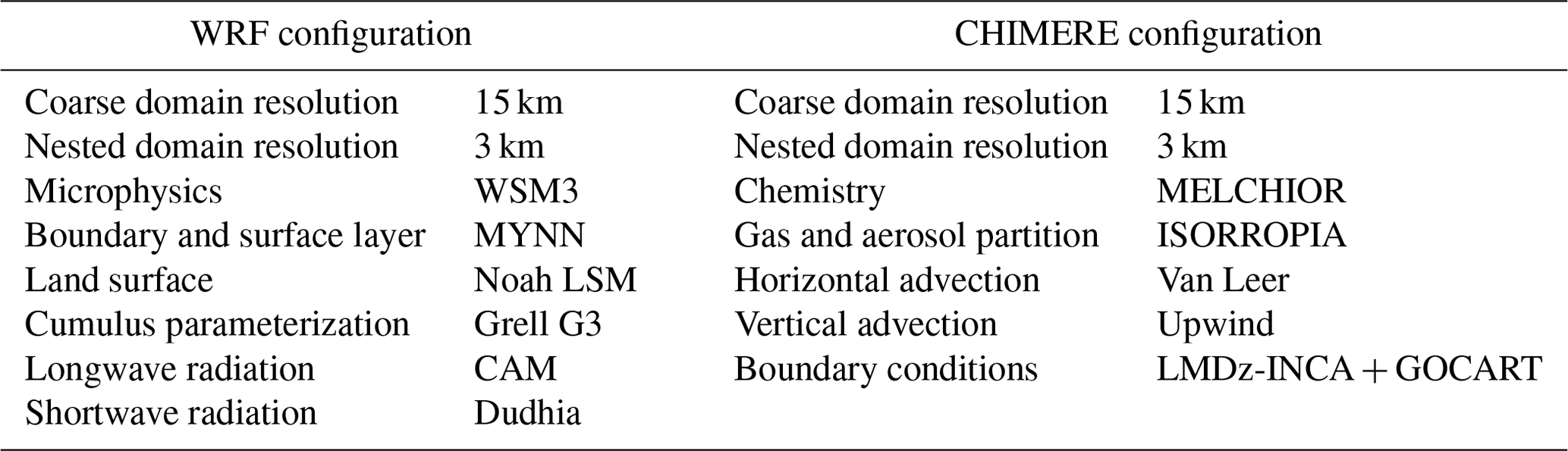
The chemistry-transport simulations are based on the combination of the Weather Research and Forecasting (WRF) mesoscale numerical weather model, EDGAR-HTAP anthropogenic emissions inventory, and CHIMERE chemistry-transport model. The simulation domains are described in Fig. 1, with a coarse domain at a 15 km spatial resolution comprising most of Chile and a nested domain focusing on central Chile and centered on Santiago at a 3 km resolution. The meteorological conditions are simulated using the WRF model from the US National Center for Atmospheric Research (Skamarock et al., 2008). The model configuration used in this study to simulate and reproduce observed meteorological conditions is presented in Table 1. The model was applied to 46 vertical levels up to the highest elevation of 50 hPa, in a two-way nested fashion, with 1-2-1 smoothing. Initial and boundary conditions used are from the NCEP FNL analysis, with a 1∘ by 1∘ spatial resolution and 6 h temporal resolution, from the Global Forecast System (NCEP, 2000). Land use and orography are based on the modified IGBP MODIS 20-category database with a 30 s resolution (University of Maryland, 2010). The simulated period is 1 June to 15 July 2016. The starting period from 1 to 15 June is used for spin-up and will not be analyzed. CHIMERE is an Eulerian three-dimensional regional chemistry-transport model that is able to reproduce gas-phase chemistry, aerosols formation, transport, and deposition. In this study the 2017 off-line version of CHIMERE is used (Mailler et al., 2017). The configuration used for this study is described in Table 1. Land-use and orography data are the same as for WRF. For anthropogenic emissions, the HTAP V2 dataset is used which consists of 0.1∘ gridded maps of air pollutant emissions for the year 2010 (Janssens-Maenhout et al., 2015). A downscaling is applied to this inventory based on land-use and demographic characteristics, and monthly emissions are split in time down to daily and hourly rates following the methodology of Menut et al. (2013).
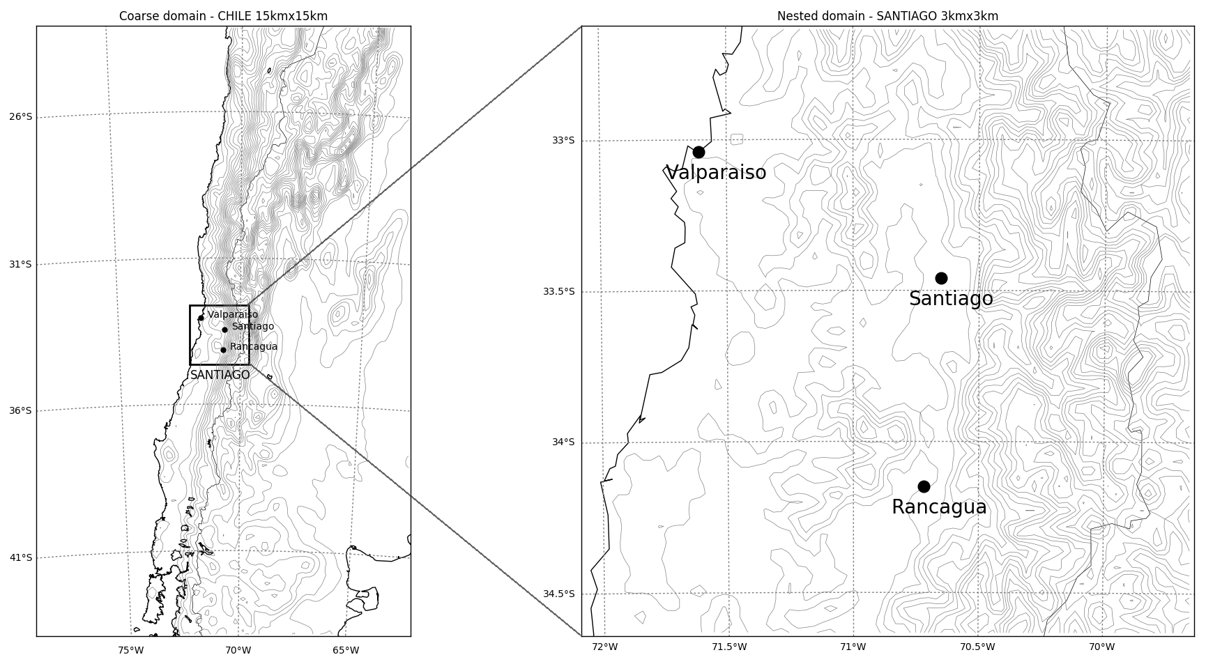
Figure 1Left panel: coarse simulation domain at a 15 km resolution. Right panel: nested domain at a 3 km resolution. The 250 m contour levels shown are interpolated from the modified IGBP MODIS 20-category database with a 30 s resolution (University of Maryland, 2010).
2.3 Simulation validation
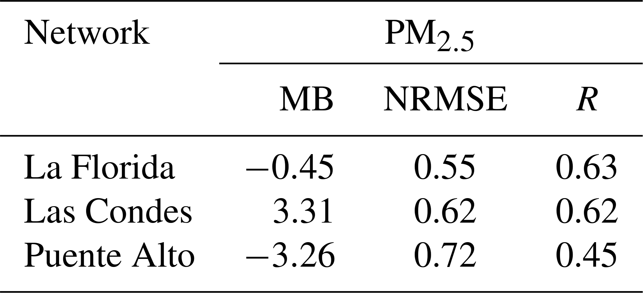
Simulation scores are gathered in Tables 2–4. Two stations downtown are used to validate the simulated near-surface meteorology (Table 2). Biases (MB) for temperature are around ±1 ∘C with correlations (R) around 0.85. The model is a little too dry with relative humidity biases between −12 % and −16 % but mostly reproduces the diurnal cycle with correlations of 0.62 and 0.7. A 10 m wind speed time series is reproduced fairly well with mean biases of −0.08 m s−1 (8 %) and 0.23 m s−1 (32 %), respectively, for observed average values of 1.04 and 0.70 m s−1 and correlations of 0.56 and 0.7. Vertical meteorological profiles scores are shown in Table 3. For the 3 d presented the statistics are satisfactory. Typical daily average concentrations of PM2.5 are reproduced quite well by the model. Table 4 gathers the scores for PM2.5 for some stations between 28 June and 15 July so as to avoid the peaks that do not represent business-as-usual conditions. Mean biases are less than 5 µg m−3, compared with average hourly levels over the period of between 35 and 55 µg m−3 for these stations. Corresponding correlations are between 0.45 and 0.63, which are decent values. The representation of wind by the model for synoptic meteorological stations in Santiago is described in Table 3 and Fig. 2. Generally speaking the model behaves well for 10 m values and profiles of wind speed and direction, so transport should be realistically represented.

Figure 2Modeled (a, b) and observed (c, d) wind rose between 15 and 30 June 2016 – synoptic stations Pudahuel and Quinta Normal.
Table 2Simulation scores – mean bias (MB), normalized root mean square error (NRMSE), and Pearson correlation (R) – for 2 m temperature (TEMP), surface relative humidity (RH) and 10 m wind speed (WS), 15 June to 15 July 2016.
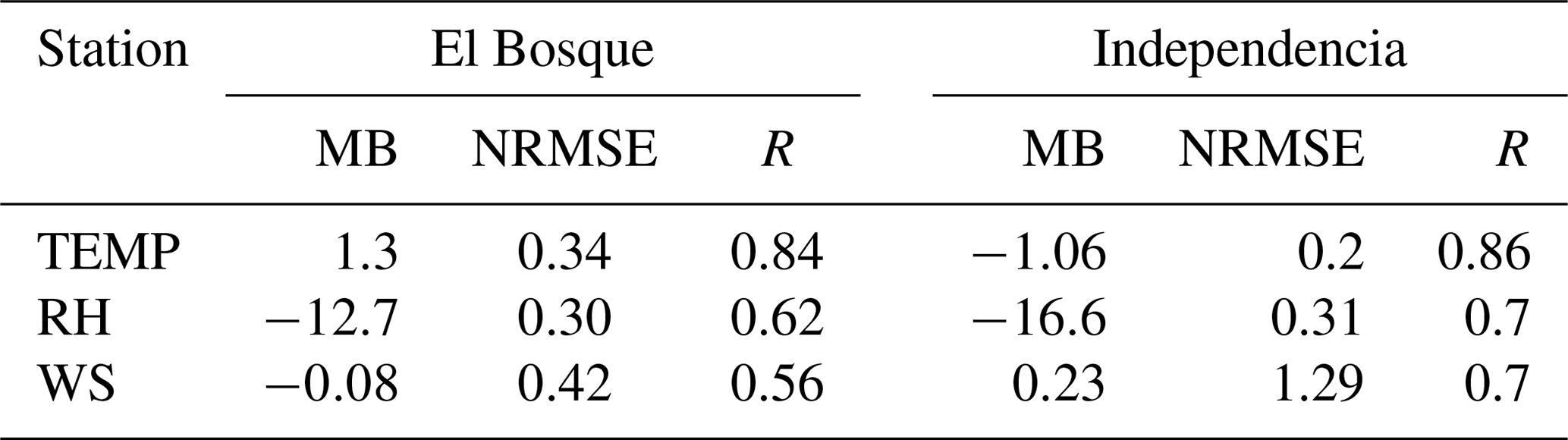
Table 3Simulation scores for meteorological vertical profiles for 3 d at DMC station in Santiago. WD is the wind direction at 10 m. All other abbreviations are the same as for Table 2.
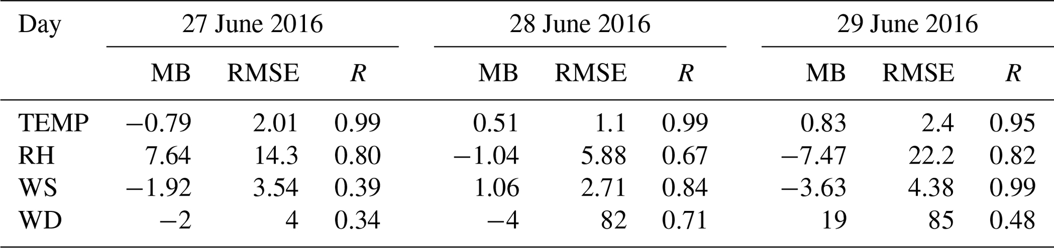
Table 4Simulation scores for low-level PM2.5 concentrations, 28 June to 15 July 2016.
The modeling setup is based on WRF-CHIMERE, with a horizontal resolution of 3 km, and emissions are downscaled from a dataset originally at a 0.1∘ resolution. At the scale of a city such as Santiago, which is roughly 20 km by 20 km, such a resolution might seem too coarse to capture the observed heterogeneity. However, the previous analysis shows that the meteorological conditions are reproduced well by the model, and the spatial distribution of PM2.5 concentrations also accounts for the observed heterogeneity (see Fig. 10 for instance). Mazzeo et al. (2018) used a similar setup with a 2 km resolution for a sensitivity analysis of traffic and residential heating emissions in Santiago, yielding similar performances. Comparable CHIMERE simulations are performed for purposes of air quality operational forecast in France, whose performance at a small scale is acknowledged in the literature, provided emissions have appropriate magnitudes (Petit et al., 2017; Shaiganfar et al., 2017).
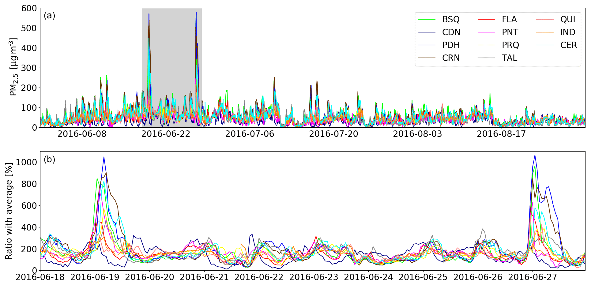
Figure 3(a) Time series of hourly PM2.5 concentration between 1 June and 31 August 2016 for the 11 stations of the air quality network of Santiago. (b) Ratio between hourly PM2.5 and average over the summer between 18 and 28 June (enlargement of shaded period in a). Stations abbreviations are as follows: BSQ – El Bosque, FLA – La Florida, QUI – Quilicura, CDN – Las Condes, PNT – Puente Alto, IND – Independencia, PDH – Pudahuel, PRQ – Parque O'Higgins, CER – Cerrillos, CRN – Cerro Navia, and TAL – Talagante.
3.1 PM2.5 peaks description
The following analysis is based on the data provided by the Sistema de Información Nacional de Calidad del Aire (SINCA) network of surface air quality sensors distributed in the metropolitan area of Santiago (Ministerio del Medio Ambiente, 2018). The time series of PM2.5 concentrations for each of the 11 stations of this network for June and July 2016 are illustrated in Fig. 3. Two skyrocketing peaks, up to 10 times higher than the average concentration for the season, occurred at several stations during the nights between 18 and 19 and 26 and 27 June. These two peaks reached all-time record-breaking levels for some stations in the city according to the available SINCA time series. Other stations show less extreme peaks, which is representative of the rich dynamics of particulate matter within Santiago (Toledo et al., 2018). Understanding the origin and modeling the dispersion of these time-limited, very sharp events are the purposes of this study. For the following analysis, the peak on 26–27 June is considered, although the analysis and results are the same for 18–19 June. Its spatial evolution can be found in Fig. 4, showing that the episode starts simultaneously at several air quality stations at around 20:00 local time (LT), with levels decreasing back to regular values the next morning. The western part of the city seems much more affected by the event than the eastern part. This comes from the diurnal wind cycle in Santiago, which features prevailing easterlies during the nighttime contributing to the renewal of air masses in this part of the city (Rutllant and Garreaud, 1995).
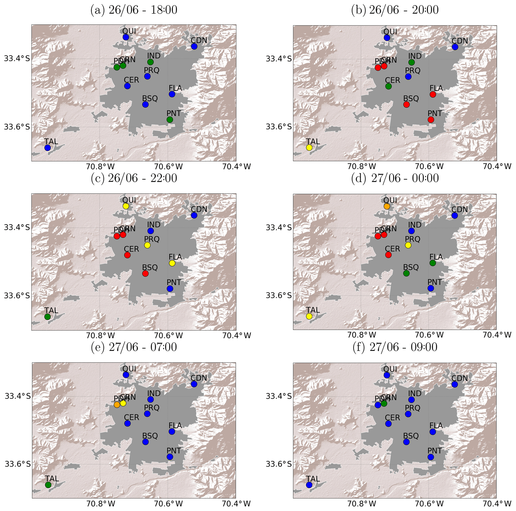
Figure 4Observed PM2.5 hourly concentrations during the peak on 26 June compared to its average over summer 2016 – blue ≤ 200 %, green ≤ 300 %, yellow ≤ 400 %, orange ≤ 500%, red > 500 %. Map background layer: World Shaded Relief, © 2009 ESRI.
The meteorological conditions observed at the location of the strongest peak during our period of interest are shown in Fig. 5. Red lines correspond to the measurements between 26 June 06:00 LT and 27 June 05:00 LT, which comprise a peak event. Figure 5a and b show that at the location of the strongest PM2.5 peak, the surface temperature and relative humidity cycles over the duration of the event are very close to the average over the month (black line). Wind speed – Fig. 5c – is a little slower than average on the whole but remains in the range of the first and third quartiles of ventilation conditions (dashed blue lines). Ceilometer profiles and boundary layer height (BLH) estimation based on the methods from Muñoz and Undurraga (2010) derived for each day at 15:00 LT – white diamonds in Fig. 5d – indicate that the mixed layer is rather shallow around the peak but not shallower than on 22–23 June for instance, which did not feature such an event. On 26 June, the mixed layer is 430 m high, which is close to the average height over the period and much higher than the minimum value (260 m) obtained on 21 June.
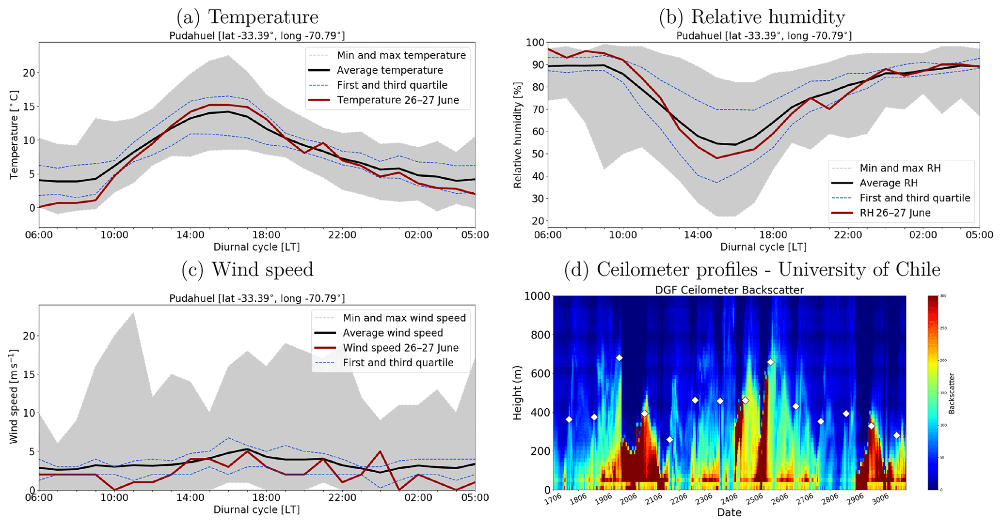
Figure 5Meteorological conditions around 26–27 June PM2.5 episode for the synoptic station Pudahuel. (a–c) Average (black line), minima and maxima (gray area), and 25th and 75th percentiles (dashed blue line) between 15 June and 15 July 2016. The red lines show the values for 26 June 06:00 LT to 27 June 05:00 LT. (d) Department of Geophysics (DGF) ceilometer hourly backscatter profiles from 17 June through 30 June 2016 and mixed-layer height at 15:00 LT (diamond white markers).
Hence, measurements show that the meteorological conditions during the peak are not very different from other days of the period, when no PM peak was recorded. Thus, meteorological conditions are not to be considered as the main forcing for the PM2.5 event although they are favorable for it to appear, which is usual for the season in the area of Santiago.
Besides meteorology, advection of a PM plume over the city could be a candidate cause for such events. For instance, wildfires occurring in the forests surrounding the city occasionally explain major peaks of particulate matter in Santiago (Rubio et al., 2015; de la Barrera et al., 2018), but these events mostly take place in the austral summer, and no such event was reported during our period of study. In addition, the strong concentration gradients observed between nearby stations (Figs. 3 and 4) make advection unlikely to be responsible for these events.
Once meteorology and transport are ruled out as root causes, high local emissions must then be underlying the very strong concentrations recorded.
3.2 Chemical signature and source identification
In order to identify the type of source involved in the sporadic peaks, Fig. 7 shows a scatterplot of PM2.5, NOx, and CO hourly surface concentrations from 15 to 30 June 2016, for the Pudahuel air quality station. Red dots correspond to PM2.5 concentrations higher than 200 µg m−3, and blue dots correspond to concentrations below that value. Out of simplicity, from now on we will refer to the former as PPE (PM peak events) and to the latter as PRS (PM regular situation). Two different regimes can be identified: for PPE, the NOx∕CO ratio is around 4.6 %, while for PRS, it is approximately 14 %. The same goes for the NOx∕PM2.5 ratio, with values of around 73 % for PPE and 502 % otherwise. Given the short-lived character of the events considered, such different concentration ratios can be related to different emission factors as discussed in Sect. 4. Thus, two different types of source are involved in the two situations considered (PPE and PRS).
Mazzeo et al. (2018) found a NOx∕PM2.5 ratio of 526 % for Pudahuel station in July 2015, without peak events. Using the same methodology and combining data from July 2015 and 2016, without peak events, we recover a concentration ratio of around 557 % for this same station. For NOx∕CO we find it is around 14 % (see Fig. 6). These two values correspond to the average pollution situation in this part of the city, i.e., what is usually observed in wintertime when no peak event occurs. They are comparable to what can be observed in PRS in Fig. 7 with an average ratio of 502 % for NOx∕PM2.5 and 14 % for NOx∕CO. Therefore, the PM regular situation (PRS) corresponds fairly well to the average situation in Santiago in winter. Peak events (PPE – red dots) however show very different ratios that do not coincide with the average situation, hence pointing to another specific source. Major contributors to atmospheric pollution in Santiago are traffic (39 %), industry (18 %), and residential heating (20 %) (Barraza et al., 2017). Based on the current Euro 5 legislation for car engine emissions in place in Chile (Ministerio del Medio Ambiente, 2017) and the vehicles fleet in Santiago (Instituto Nacional de Estadísticas, 2016), the expected emission ratio from traffic yields around 12 % for NOx∕CO and 1680 % for NOx∕PM2.5. Similarly, emission ratios extracted from the HTAP inventory for traffic at the grid point corresponding to Santiago yield 7.5 % for NOx∕CO and 1750 % for NOx∕PM2.5. This does not match with the PPE signal, especially regarding NOx and PM2.5. For residential heating, the HTAP inventory gives emission ratios at the grid point of Santiago of 19 % for NOx∕CO and 200 % for NOx∕PM2.5, also departing from the values observed during PPE. In addition, residential heating by the domestic combustion of wood and/or fossil fuel is expected to have slow variations in time, depending essentially on outside temperature (Saide et al., 2016), which as discussed above was not particularly colder on peak days than on other days, permitting us to rule out residential heating as the main contribution to these short-lived peaks. Industrial emissions are also generally constant through time, thereby excluding the possibility that they could be the main factor too. HTAP emission ratios for industry also significantly differ from the PPE situation, with 20 % for NOx∕CO and 186 % for NOx∕PM2.5. Sources other than usual ones must therefore cause these peaks.
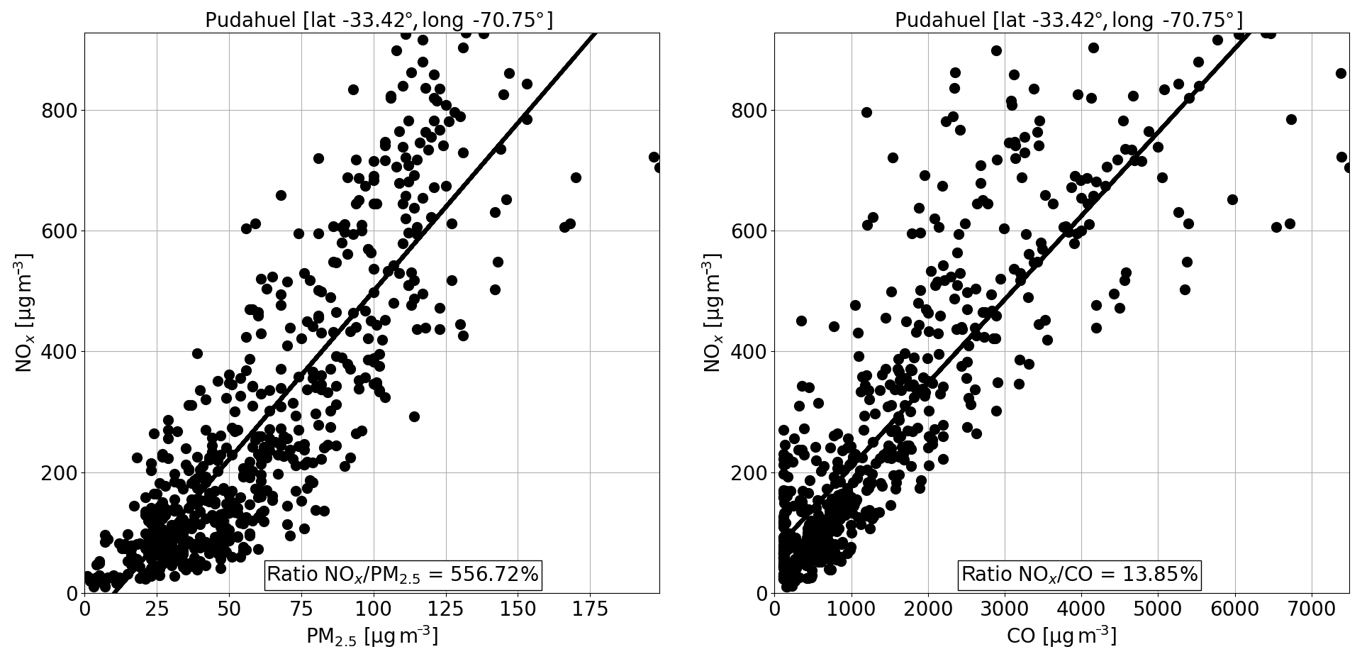
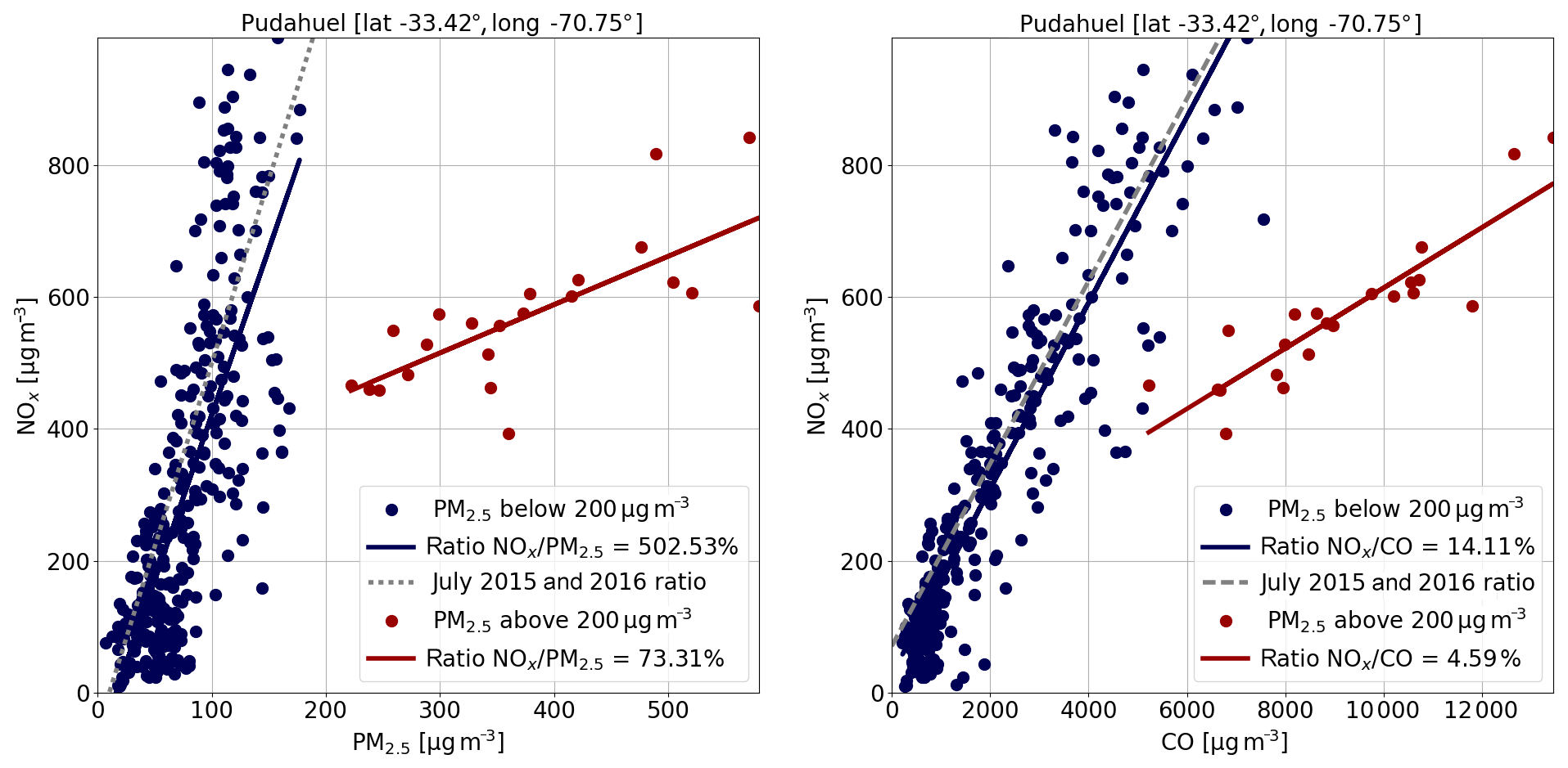
Figure 7Observed NOx∕CO and NOx∕PM2.5 concentration ratios at Pudahuel station (PDH). Blue dots are for PM2.5 concentrations below 200 µg m−3; red dots are for PM2.5 concentrations above 200 µg m−3; gray line represents the ratio for July 2015 and 2016; blue and red lines correspond to linear regressions for each dataset.
Since the peak events considered occurred exclusively during evenings and nights, cooking emissions such as barbecues, which are a cultural habit in Chile, could be a candidate. Different studies estimate emission factors from barbecue cooking (charcoal only and including meat emissions), from which ratios of 1.4 % (Vicente et al., 2018) to 2.4 % (Lee, 1999) for NOx∕CO and 40.5 % (Vicente et al., 2018) to 61.5 % (Lee, 1999) for NOx∕PM2.5 can be derived. These numbers are not far from the 4.6 % and 73 % observed during PPE (Fig. 7), suggesting that, although the atmospheric composition is likely the result of multiple sources, the main signal in the observed PM2.5 concentrations corresponds to emissions from barbecues. As a first-order approximation, we use emission ratios and concentration ratios equivalently. This assumption is examined in Sect. 4. However, one question remains: why would there be peaks of barbecue cooking on the nights of 18 and 26 June specifically, rather than on other nights during the studied period? This question is even more pertinent given that barbecues are mainly a spring–summer activity in Chile.
Usually, barbecues (or asados) are cooked when celebrating particular events in Chile. So as to gain statistical significance by including more events, the time period studied was expanded to winter 2015 and 2014 as well. As it turns out, during the month of June in these 3 years, eight episodes with hourly PM2.5 higher than 200 µg m−3 were recorded at Pudahuel station, five of which peaked during international soccer games involving the Chilean national team. The three others were declared within 24 h of a game. It is even clearer for peaks higher than 400 µg m−3, all of them occurring at the exact same hour as the kickoff of a soccer game when the next day was not a working day – see Fig. 8 in which red diamonds represent Chile game kickoffs during the 2014 FIFA World Cup, 2015 Copa América, and 2016 Copa América. In addition, for the recent years without a major soccer championship involving the team of Chile (i.e., 2010, 2012, 2013, 2017), the maximum hourly PM2.5 concentration at Pudahuel over the same period of the year was 260 µg m−3. In 2011 another Copa América was held, and values reached up to 360 µg m−3.
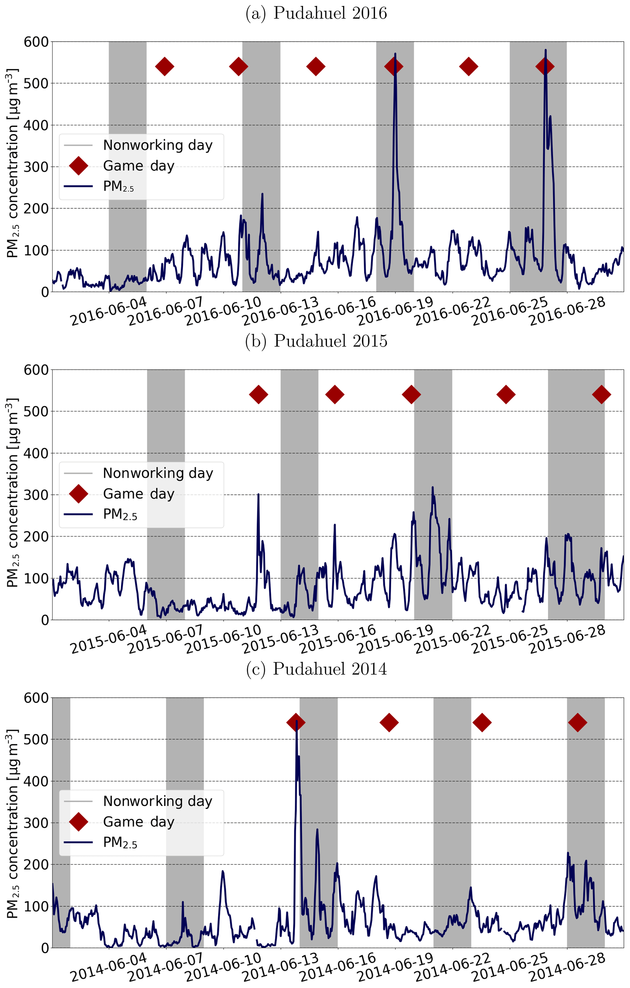
Figure 8PM2.5 peak events coincidence with soccer games. (a) Hourly PM2.5 concentrations at Pudahuel monitoring station (solid blue line), kickoff hours of soccer games (red diamonds), and nonworking days (shaded gray areas) in June 2016. (b) Same as (a) for June 2015. (c) Same as (a) for June 2014. Dates are given in the format year-month-day.
This correlation is likely not coincidental. Over the months of June 2014, 2015, and 2016, the observations show 12 d recording pre-emergency conditions (24 h PM2.5 concentration above 110 µg m−3). Among these 12 d, 10 dates coincided with a soccer game of the national team or the day after such a game (games being played at nights, the peak affects both the game day and the day after). The three periods total 90 d, 15 of which were game days. Based on combinatorics, the probability that soccer games and PM2.5 pre-emergency levels coincidentally occur with a proportion of at least 10 out of 12 can be expressed as in Eq. (1). This corresponds to randomly drawing 15 d out of the 90 available and obtaining at least 10 peaks. As a result, the probability that the correlation between PM2.5 peaks and soccer games is purely coincidental is 0.002 %. Thus we can be confident that there is actually a significant correlation between these two types of events, caused by massive barbecue cooking during games.
The observations made in Fig. 7 are also valid for other stations throughout the city. Figure 9 shows the NOx∕CO and NOx∕PM2.5 ratios for three other locations in Santiago, distinguishing between the hours around the games of 18 and 26 June (red dots) and the other data for the month (blue dots). Again, two different regimes are observed, with the one during games being attributable to barbecues based on the same analysis as previously carried out, although barbecues seem to be even more dominant in Pudahuel. In summary, we have shown here that major peak events of PM2.5 in Santiago are correlated with soccer games played on the evening before a nonworking day, and such conditions can be tied to massive barbecue cooking throughout the city, given the chemical footprint observed at that time.

Figure 9Observed NOx∕CO and NOx∕PM2.5 concentration ratios at three stations in June 2016. Blue dots are observations during the 18 and 26 June soccer games. Red dots correspond to the rest of the data. Dashed blue and red lines correspond to linear regressions for each case.
3.3 Transport
These barbecue peaks, although generating large amounts of PM2.5, last only a few hours. The termination of one of these events is studied hereafter. A chemistry-transport simulation is run with WRF (Skamarock et al., 2008) and CHIMERE (Mailler et al., 2017) for the austral winter 2016 (see Sect. 2 for the details). A first baseline simulation aiming to reproduce observed concentrations of pollutants is performed using the HTAP anthropogenic emissions inventory (Janssens-Maenhout et al., 2015). This inventory does not account for sporadic emissions such as the ones studied here. Despite a good performance in reproducing the observed meteorology and atmospheric composition (see Sect. 2, Tables 2–4), the model does not produce peak events on 18 and 26 June (dashed black line in Fig. 10). This reinforces the idea that strong sporadic emissions are actually at play rather than extreme weather conditions. In a second simulation, all other things remaining equal, strong additional sources of PM2.5 are added all over the city based on population density and plugged into CHIMERE in order to account for barbecues being cooked on 26 June.
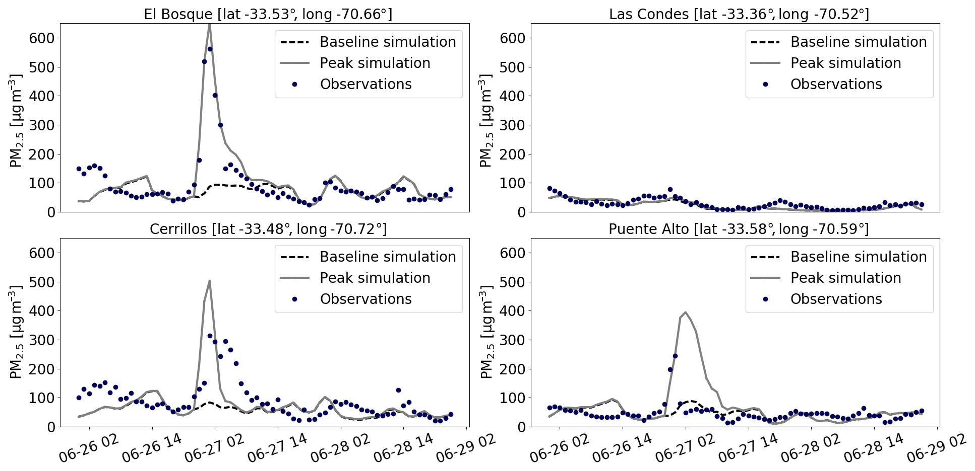
Figure 10Observed (blue dots) and simulated (baseline simulation is dashed black line; peak simulation is gray line) PM2.5 surface concentrations time series at four stations in Santiago around the peak episode of 26 June 2016.
A survey conducted before the final game of the 2016 Copa América estimated that 29 % of Santiago's inhabitants would cook a barbecue during the game (Panel Ciudadano de la Universidad del Desarrollo, 2016). As a first-order approximation, considering only the adult population and assuming that this is a group activity gathering on average seven people, we estimate that this corresponds to 100 000 fires that were lit at the time of the game. Based on PM emission rates estimated by the US Environmental Protection Agency (Lee, 1999) at around 20 g h−1 on average, with variations depending on the type of meat cooked, the expected additional emission of PM2.5 would be a total of 2 t h−1 for the whole region. In a heavily populated area such as El Bosque, this represents an additional signal 15 times higher than the PM2.5 emission rate used in the baseline simulation. We acknowledge the multiple sources of uncertainty in this estimation. However our goal is to explore barbecues as a potential significant source of PM2.5 pollution, which only requires orders of magnitude given the strength of the signal. Barbecues are assumed to last 3 h starting 1 h before the game kickoff. The estimated additional emissions are plugged into CHIMERE for the peak simulation (gray line in Fig. 10).
The resulting PM2.5 concentration time series in Fig. 10 shows that the observations are reproduced well using this proxy in the south (El Bosque) and northeast (Las Condes). Although the magnitude is a little overestimated but not far off, the time evolution of concentrations is reproduced less well in the west (Cerrillos), where the peak is too short, and in the southeast (Puente Alto), where it lasts too long. This is possibly due to the representation of slope winds by the model: too weak easterlies coming from the Andes in the simulation would result in not enough ventilation in the east (i.e., a peak that lasts too long) and not enough accumulation in the west (i.e., a too short-lived event). Not many observations are available to investigate this hypothesis. Generally speaking, the peak simulation confirms the magnitude of our estimate of 100 000 barbecues cooked during the game or an additional 6 t of PM2.5 emitted in total for the area.
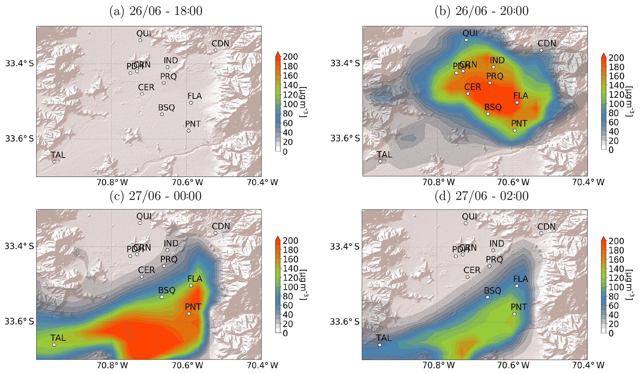
Figure 11PM2.5 concentration difference at 60 m above the surface between the peak event and baseline simulation on 26–27 June. Positive values indicate excess concentrations in the peak event scenario compared to the baseline. Map background layer: World Shaded Relief, © 2009 ESRI.
Based on this simulation, the transport of the particles generated by the barbecue events can also be studied. Figures 11 and 12 show the difference in PM2.5 concentration between the two simulations aforementioned, for the peaks on 26 and 18 July, respectively. Concentrations at 60 m a.g.l. (above ground level) are considered in order to get rid of the signal of emissions. The simulations result in an evacuation of the particles towards the southwest of Santiago for both events, a few hours after the onset. Again the episodes are short-lived in the city but have impacts on adjacent areas several hours later and several kilometers away from the emission site. For both events the areas impacted by the dispersion of the plume are the south and southwest regions. Although this result is consistent with mountain–valley circulation, it does not imply that such a dispersion pattern is the only one that can occur during peak events. In addition to the impact within the city, collateral effects outside Santiago must be studied in greater detail, such as a potential deposition of the particles on crops, with effects on yields, or on adjacent glaciers, with radiative effects.
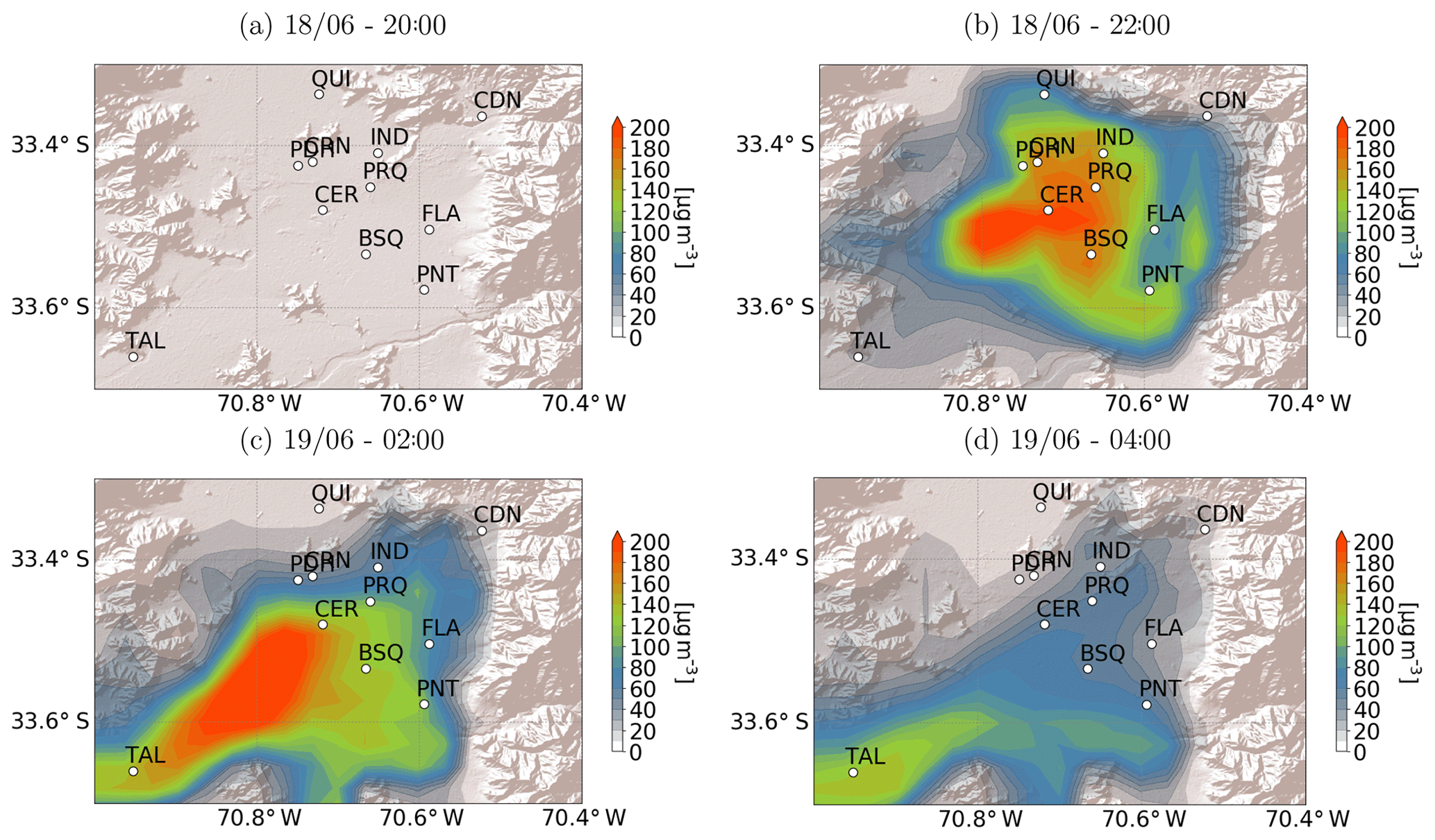
Figure 12PM2.5 concentration difference at 60 m above the surface between the peak event and baseline simulation on 18–19 June. Positive values indicate excess concentrations in the peak event scenario compared to the baseline. Map background layer: World Shaded Relief, © 2009 ESRI.
In Sect. 3.2, the conclusions are based on the approximation that the concentration ratios observed correspond to the ratios of the underlying emission factors. Chemical processes are at play in the atmosphere that can lead to a difference between these two variables though. However atmospheric lifetimes of NOx and CO (respectively, 1 to 10 d and 1 to 4 months; Seinfeld and Pandis, 2006) are too long for these species to be significantly removed during the few hours we focus on. The NOx∕CO ratio at emission and concentration ratio are thus expected to be very close. For particulate matter, the discussion is less clear. Secondary PM can form, adding to the emitted PM2.5. The nucleation of secondary PM would lead to a NOx∕PM2.5 concentration ratio smaller than the emission ratio. However, 1 order of magnitude separates the two regimes we observe, and the timescale we study does not leave much time for secondary PM to become significant, implying a small contribution to the total PM (for instance the apportionment of secondary versus primary aerosols in our baseline simulation varies between 4 % and 63 % with an average value of 33 %).
In the last few decades, decontamination plans in Santiago have mainly focused on decreasing emissions from traffic, industry, and residential heating. The chemical footprint of extreme peak events evidenced in this study advocates in favor of also considering more specific and sporadic sources based on cultural habits such as barbecues. Indeed, the mitigation policies currently implemented are helping to lower pollution levels but, based on our study, cannot prevent extreme PM2.5 events from happening, whose impact can be significant as well. The “game effect” phenomenon has been hypothesized by local authorities but had not previously been backed up by scientific evidence. An analysis of the time characteristics of the events showed that they happen exclusively during soccer games of the national team, played in evenings before a nonworking day. The observed concentrations of NOx, CO, and PM2.5 at that time, compared with the usual levels, allow for us to trace back the main contribution to fine particles emitted by barbecue cooking. The number of barbecues cooked during one peak event is estimated, and the associated emissions are plugged into a chemistry-transport simulation, leading to the reproduction of the observed peaks, which is not the case without these emissions. The model then yields appropriate levels, thus confirming the estimated emissions and allowing for the study of the evacuation of the PM2.5 plume towards the southwest of the metropolitan area. The more general question of the fate and impacts of particulate matter plumes generated in Santiago is raised.
Although the results provided here seem to have geographically limited implications, the general methodology can be reproduced and benefit other places in the world. Indeed, using only a limited set of data, with no speciation of particulate matter, already enables us to determine the source of extreme events, provided they are tied to cultural habits differing from the usual sources of air pollution. Such types of sporadic habits are usually ignored by air quality plans implemented by cities, due to the lack of scientific evidence.
In addition, a model-based approach allowed for us to constrain the estimate of number of barbecues cooked during the final game of the 2016 Copa América (around 100 000). Not only can this result have an informative value for local authorities but also such a sensitivity analysis can be reproduced and applied to other cases throughout the world in order to estimate the burden on air quality of specific sources.
The CHIMERE model used can be found at http://www.lmd.polytechnique.fr/chimere/CW-download.php (last access: 14 April 2020) (École Polytechnique, 2020). The WRF model used can be found at http://www2.mmm.ucar.edu/wrf/users/download/get_source.html (last access: 14 April 2020) (University Corporation for Atmospheric Research, 2012).
Surface observation data used in this study are available at https://sinca.mma.gob.cl/index.php/region/index/id/M (last access: 14 April 2020) (Ministerio del Medio Ambiente, 2012). The HTAP raw emission inventory can be downloaded at http://edgar.jrc.ec.europa.eu/htap_v2/ (last access: 14 April 2020) (European Commission, 2020). Other data can be made available from the corresponding author upon reasonable request.
NH provided meteorological profiles data and synoptic stations wind speeds used to assess the quality of the simulation. As developers of CHIMERE, LM and SM supervised the chemistry-transport simulations and analyses of the results. RL performed the data analysis and model simulations and coordinated the writing of the paper with LM, SM and, NH.
The authors declare that they have no conflict of interest.
The authors are grateful to Ricardo C. Muñoz for providing them with the ceilometer backscatter profiles and mixed-layer height computations used in the meteorological analysis. Nicolás Huneeus acknowledges the project FONDECYT Regular 1181139. The chemistry-transport simulations used in this work were performed using the high-performance computing resources of TGCC (Très Grand Centre de Calcul du CEA) under the allocation GEN10274 provided by GENCI (Grand Équipement National de Calcul Intensif). The authors wish to thank the editor as well as the two anonymous reviewers for their constructive comments during the discussion phase.
This paper was edited by Maria Kanakidou and reviewed by two anonymous referees.
Barraza, F., Lambert, F., Jorquera, H., Villalobos, A. M., and Gallardo, L.: Temporal evolution of main ambient PM2.5 sources in Santiago, Chile, from 1998 to 2012, Atmos. Chem. Phys., 17, 10093–10107, https://doi.org/10.5194/acp-17-10093-2017, 2017. a, b
de la Barrera, F., Barraza, F., Favier, P., Ruiz, V., and Quense, J.: Megafires in Chile 2017: Monitoring multiscale environmental impacts of burned ecosystems, Sci. Total Environ., 637–638, 1526–1536, https://doi.org/10.1016/j.scitotenv.2018.05.119, 2018. a
École Polytechnique: CHIMERE Registration Form, available at: http://www.lmd.polytechnique.fr/chimere/CW-download.php, last access: 17 April 2020. a
Energy Policy Institute at the University of Chicago: Air Quality Life Index, available at: https://aqli.epic.uchicago.edu/ (last access: 10 September 2019), 2017. a
European Commission: EUROPA – EDGAR FOR HTAP V2, available at: http://edgar.jrc.ec.europa.eu/htap_v2/, last access: 17 April 2020. a
Gallardo, L., Barraza, F., Ceballos, A., Galleguillos, M., Huneeus, N., Lambert, F., Ibarra, C., Munizaga, M., O'Ryan, R., Osses, M., Tolvett, S., Urquiza, A., and Véliz, K. D.: Evolution of air quality in Santiago: The role of mobility and lessons from the science-policy interface, Elem. Sci. Anth., 6, 38–61, https://doi.org/10.1525/elementa.293, 2018. a
Ilabaca, M., Olaeta, I., Campos, E., Villaire, J., Tellez-Rojo, M. M., and Romieu, I.: Association between Levels of Fine Particulate and Emergency Visits for Pneumonia and other Respiratory Illnesses among Children in Santiago, Chile, J. Air Waste Manage., 49, 154–163, https://doi.org/10.1080/10473289.1999.10463879, 2011. a
Instituto Nacional de Estadísticas: Anuarios Parque de Vehiculos en Circulacion, availalbe at: http://historico.ine.cl/canales/chile_estadistico/estadisticas_economicas/transporte_y_comunicaciones/parquevehiculos.php (last access: 10 September 2019), 2016. a
Janssens-Maenhout, G., Crippa, M., Guizzardi, D., Dentener, F., Muntean, M., Pouliot, G., Keating, T., Zhang, Q., Kurokawa, J., Wankmüller, R., Denier van der Gon, H., Kuenen, J. J. P., Klimont, Z., Frost, G., Darras, S., Koffi, B., and Li, M.: HTAP_v2.2: a mosaic of regional and global emission grid maps for 2008 and 2010 to study hemispheric transport of air pollution, Atmos. Chem. Phys., 15, 11411–11432, https://doi.org/10.5194/acp-15-11411-2015, 2015. a, b
Lee, S. Y.: Emissions from street vendor cooking devices (charcoal grilling), Tech. rep., United States Environmental Protection Agency, Washington, D.C., 1999. a, b, c
Mailler, S., Menut, L., Khvorostyanov, D., Valari, M., Couvidat, F., Siour, G., Turquety, S., Briant, R., Tuccella, P., Bessagnet, B., Colette, A., Létinois, L., Markakis, K., and Meleux, F.: CHIMERE-2017: from urban to hemispheric chemistry-transport modeling, Geosci. Model Dev., 10, 2397–2423, https://doi.org/10.5194/gmd-10-2397-2017, 2017. a, b
Mazzeo, A., Huneeus, N., Ordoñez, C., Orfanoz-Cheuquelaf, A., Menut, L., Mailler, S., Valari, M., van der Gon, H. D., Gallardo, L., Muñoz, R., Donoso, R., Galleguillos, M., Ossesa, M., and Tolvett, S.: Impact of residential combustion and transport emissions on air pollution in Santiago during winter, Atmos. Environ., 190, 195–208, https://doi.org/10.1016/j.atmosenv.2018.06.043, 2018. a, b, c, d
Menut, L., Bessagnet, B., Khvorostyanov, D., Beekmann, M., Blond, N., Colette, A., Coll, I., Curci, G., Foret, G., Hodzic, A., Mailler, S., Meleux, F., Monge, J.-L., Pison, I., Siour, G., Turquety, S., Valari, M., Vautard, R., and Vivanco, M. G.: CHIMERE 2013: a model for regional atmospheric composition modelling, Geosci. Model Dev., 6, 981–1028, https://doi.org/10.5194/gmd-6-981-2013, 2013. a
Ministerio del Medio Ambiente: Análisis General para el Impacto Económico y Social (AGIES) de la Norma de Calidad Primaria de Material Particulado 2.5, Tech. rep., MMA, available at: http://planesynormas.mma.gob.cl/archivos/2014/proyectos/235_6__Folio_N_881_al_1008.pdf (last access: 10 September 2019), 2012. a, b
Ministerio del Medio Ambiente: Establece Plan de Prevención y Descontaminación Atmosférica para la Región Metropolitana de Santiago, available at: https://www.leychile.cl/N?i=1111283&f=2017-11-24&p= (last access: 10 September 2019), 2017. a
Ministerio del Medio Ambiente: Sistema de Información Nacional de Calidad del Aire, available at: https://sinca.mma.gob.cl/index.php/ (last access: 17 April 2020), 2018. a
Ministerio del Medio Ambiente: Región Metropolitana de Santiago – Sistema de Información Nacional de Calidad del Aire, available at: https://sinca.mma.gob.cl/index.php/region/index/id/M, last access: 17 April 2020. a
Muñoz, R. C. and Undurraga, A. A.: Daytime Mixed Layer over the Santiago Basin: Description of Two Years of Observations with a Lidar Ceilometer, J. Appl. Meteorol. Clim., 49, 1728–1741, https://doi.org/10.1175/2010JAMC2347.1, 2010. a
NCEP: NCEP FNL Operational Model Global Tropospheric Analyses, continuing from July 1999, Boulder, Colorado, https://doi.org/10.5065/D6M043C6, 2000. a
Panel Ciudadano de la Universidad del Desarrollo: Santiaguinos esperan con altas expectativas el partido de hoy … y un 29 % hará asado, El Mercurio, available at: https://gobierno.udd.cl/cpp/noticias/2017/01/17/santiaguinos-esperan-con-altas-expectativas-el-partido-de-hoy (last access: 10 September 2019), 2016. a
Petit, J.-E., Amodeo, T., Meleux, F., Bessagnet, B., Menut, L., Grenier, D., Pellan, Y., Ockler, A., Rocq, B., Gros, V., Sciare, J., and Favez, O.: Characterising an intense PM pollution episode in March 2015 in France from multi-site approach and near real time data: Climatology, variabilities, geographical origins and model evaluation, Atmos. Environ., 155, 68–84, https://doi.org/10.1016/j.atmosenv.2017.02.012, 2017. a
Rubio, M. A., Lissi, E., Gramsch, E., and Garreaud, R. D.: Effect of Nearby Forest Fires on Ground Level Ozone Concentrations in Santiago, Chile, Atmosphere, 6, 1926–1938, https://doi.org/10.3390/atmos6121838, 2015. a
Rutllant, J. and Garreaud, R.: Meteorological Air Pollution Potential for Santiago, Chile: Towards an Objective Episode Forecasting, Environ. Monit. Assess., 34, 223–244, https://doi.org/10.1007/BF00554796, 1995. a, b, c
Saide, P. E., Mena-Carrasco, M., Tolvett, S., Hernandez, P., and Carmichael, G. R.: Air quality forecasting for winter-time PM2.5 episodes occurring in multiple cities in central and southern Chile, J. Geophys. Res.-Atmos., 121, 558–575, https://doi.org/10.1002/2015JD023949, 2016. a, b
Seinfeld, J. H. and Pandis, S. N.: Atmospheric Chemistry and Physics: From Air Pollution to Climate Change, 2nd Edn., John Wiley & Sons, Inc., Hoboken, New Jersey, 2006. a
Shaiganfar, R., Beirle, S., Denier van der Gon, H., Jonkers, S., Kuenen, J., Petetin, H., Zhang, Q., Beekmann, M., and Wagner, T.: Estimation of the Paris NOx emissions from mobile MAX-DOAS observations and CHIMERE model simulations during the MEGAPOLI campaign using the closed integral method, Atmos. Chem. Phys., 17, 7853–7890, https://doi.org/10.5194/acp-17-7853-2017, 2017. a
Skamarock, W. C., Klemp, J. B., Dudhia, J., Gill, D. O., Barker, D. M., Duda, M. G., Huang, X.-Y., Wang, W., and Powers, J. G.: A Description of the Advanced Research WRF Version 3, NCAR Technical Note 27, NCAR, Boulder, Colorado, 2008. a, b
Toledo, F., Garrido, C., Díaz, M., Rondanelli, R., Jorquera, S., and Valdivieso, P.: AOT Retrieval Procedure for Distributed Measurements With Low-Cost Sun Photometers, J. Geophys. Res.-Atmos., 123, 1113–1131, https://doi.org/10.1002/2017JD027309, 2018. a
Toro A, R., Kvakić, M., Klaić, Z. B., Koračin, D., Morales S, R. G., and Leiva, G, M. A.: Exploring atmospheric stagnation during a severe particulate matter air pollution episode over complex terrain in Santiago, Chile, Environ. Pollut., 244, 705–714, https://doi.org/10.1016/j.envpol.2018.10.067, 2018. a
University Corporation for Atmospheric Research: WRF Modeling System Download, available at: http://www2.mmm.ucar.edu/wrf/users/download/get_source.html, last access: 17 April 2020. a
University of Maryland: GLCF: MODIS Land Cover, available at: http://glcf.umd.edu/data/lc/ (last access: 10 September 2019), 2010. a, b
Vicente, E., Vicente, A., Evtyugina, M., Carvalho, R., Tarelho, L., Oduber, F., and Alves, C.: Particulate and gaseous emissions from charcoal combustion in barbecue grills, Fuel Process. Technol., 176, 296–306, https://doi.org/10.1016/j.fuproc.2018.03.004, 2018. a, b
World Health Organization: WHO Air quality guidelines for particulate matter, ozone, nitrogen dioxide and sulfur dioxide: global update 2005: summary of risk assessment, Geneva, Switzerland, 2006. a