Background heterogeneity and other uncertainties in estimating urban methane flux: results from the Indianapolis Flux Experiment (INFLUX)

As natural gas extraction and use continues to increase, the need to quantify emissions of methane (CH₄), a powerful greenhouse gas, has grown. Large discrepancies in Indianapolis CH₄ emissions have been observed when comparing inventory, aircraft mass balance, and tower inverse modeling estimates. Four years of continuous CH₄ mole fraction observations from a network of nine towers as a part of the Indianapolis Flux Experiment (INFLUX) are utilized to investigate four possible reasons for the abovementioned inconsistencies: (1) differences in definition of the city domain, (2) a highly temporally variable and spatially non-uniform CH₄ background, (3) temporal variability in CH₄ emissions, and (4) CH₄ sources that are not accounted for in the inventory. Reducing the Indianapolis urban domain size to be consistent with the inventory domain size decreases the CH₄ emission estimation of the inverse modeling methodology by about 35 %, thereby lessening the discrepancy and bringing total city flux within the error range of one of the two inventories. Nevertheless, the inverse modeling estimate still remains about 91 % higher than inventory estimates. Hourly urban background CH₄ mole fractions are shown to be spatially heterogeneous and temporally variable. Variability in background mole fractions observed at any given moment and a single location could be up to about 50 ppb depending on a wind direction but decreases substantially when averaged over multiple days. Statistically significant, long-term biases in background mole fractions of 2–5 ppb are found from single-point observations for most wind directions. Boundary layer budget estimates suggest that Indianapolis CH₄ emissions did not change significantly when comparing 2014 to 2016. However, it appears that CH₄ emissions may follow a diurnal cycle, with daytime emissions (12:00–16:00 LST) approximately twice as large as nighttime emissions (20:00–05:00 LST). We found no evidence for large CH₄ point sources that are otherwise missing from the inventories. The data from the towers confirm that the strongest CH₄ source in Indianapolis is South Side landfill. Leaks from the natural gas distribution system that were detected with the tower network appeared localized and non-permanent. Our simple atmospheric budget analyses estimate the magnitude of the diffuse natural gas source to be 70 % higher than inventory estimates, but more comprehensive analyses are needed. Long-term averaging, spatially extensive upwind mole fraction observations, mesoscale atmospheric modeling of the regional emissions environment, and careful treatment of the times of day are recommended for precise and accurate quantification of urban CH₄ emissions.

1 Introduction

From the beginning of the Industrial Revolution to 2011, atmospheric methane (CH₄) mole fractions increased by a factor of 2.5 due to anthropogenic processes such as fossil fuel production, waste management, and agricultural activities (Ciais et al., 2013; Hmiel et al., 2020). The increase in CH₄ is a concern as it is a potent greenhouse gas (GHG) with a global warming potential 28–34 times greater than that of CO₂ over a period of 100 years (Myhre et al., 2013). The magnitudes of component CH₄ sources responsible for the recent increase in the global CH₄ budget are not well understood, with theories attributing these changes to biogenic, thermogenic, and pyrogenic emissions or a decline in the atmospheric CH₄ sink (Nisbet et al., 2016, 2019; Saunois et al., 2016; Hmiel et al., 2020). Improved understanding of CH₄ emissions is needed (National Academies of Sciences and Medicine, 2018).

In particular, the estimates of continental US anthropogenic CH₄ emissions disagree. Inventories from the Environment Protection Agency (EPA) and Emissions Database for Global Atmospheric Research (EDGAR) in 2008 reported emission values of 19.6 and 22.1 Tg C yr⁻¹ (U.S. EPA, 2013; European Commission Joint Research Centre and Netherlands Environmental Assessment Agency, 2010). However, top-down methodologies using aircraft and inverse modeling frameworks found emission values of 32.4±4.5 Tg C yr⁻¹ for 2004 and 33.4±1.4 Tg C yr⁻¹ for 2007–2008 respectively (Kort et al., 2008; Miller et al., 2013). Underestimation of natural gas (NG) production and agricultural sources are possible reasons for this disagreement (Miller et al., 2013; Brandt et al., 2014; Jeong et al., 2014). Efforts to reconcile GHG emissions estimates using atmospheric methods and inventory assessment have sometimes succeeded (Schuh et al., 2013; Zavala-Araiza et al., 2015; Turnbull et al., 2019) when careful attention is given to the details of each method, and targeted atmospheric data are available. A recent synthesis of emissions from the US NG supply chain demonstrated similar success and concluded that current inventory estimates of emissions from US NG production are too low and that emission from NG distribution is one of the greatest remaining sources of uncertainty in the NG supply chain (Alvarez et al., 2018).

Due to the uncertainties in CH₄ emissions from NG distribution it is natural that urban emissions are of interest as well. For example, two studies (McKain et al., 2015; Hendrick et al., 2016) indicate that ∼60 %–100 % of Boston CH₄ emissions are attributable to the NG distribution system. Recent studies of urban CH₄ emissions in California indicate that the California Air Resources Board (CARB) inventory tends to underestimate the actual CH₄ urban fluxes, possibly due to fugitive emissions from NG infrastructures in urban environments (Wunch et al., 2009; Jeong et al., 2016, 2017). The accuracy and precision of atmospheric estimates of urban CH₄ emissions are limited by available atmospheric observations (Townsend-Small et al., 2012), potential source magnitude variability with time (Jackson et al., 2014; Lamb et al., 2016), errors in atmospheric transport modeling (Hendrick et al., 2016; Deng et al., 2017; Sarmiento et al., 2017), and complexity in atmospheric background conditions (Cambaliza et al., 2014; Karion et al., 2015; Heimburger et al., 2017). In this work, detailed analysis of urban CH₄ mole fractions is performed for the city of Indianapolis to better understand the aforementioned uncertainties of urban CH₄ emissions.

The Indianapolis Flux Experiment (INFLUX; Davis et al., 2017) is a testbed for improving the quantification of urban GHGs emissions and their variability in space and time. INFLUX (http://influx.psu.edu, last access: 8 April 2020) is located in Indianapolis partly because of its isolation from other urban centers and the flat Midwestern terrain. It includes a very dense GHG monitoring network, comprised of irregular in situ aircraft measurements (Heimburger et al., 2017; Cambaliza et al., 2014), continuous in situ observations from communications towers using cavity ring-down spectroscopy (Richardson et al., 2017; Miles et al., 2017a), and automated flask sampling systems for the quantification of a wide variety of trace gases (Turnbull et al., 2015). Meteorological sensors include a Doppler lidar providing continuous boundary layer depth and wind profiles and tower-based eddy covariance measurements of the fluxes of momentum and sensible and latent heat (Sarmiento et al., 2017). The network is designed for emissions quantification using top-down methods such as tower-based inverse modeling (Lauvaux et al., 2016) and aircraft mass balance estimates (Cambaliza et al., 2015).

Lamb et al. (2016) compared Indianapolis CH₄ emissions estimates from a variety of approaches, specifically inventory, aircraft mass balances, and inverse modeling. The results revealed large mean differences among the city fluxes estimated from these methods (Fig. 1). In general, the inventory methods arrived at lower estimates of emissions compared to the atmospheric or top-down approaches. CH₄ fluxes calculated using the aircraft mass balance technique varied considerably between flights, more than would be expected from propagation of errors of the component measurements (Cambaliza et al., 2014; Lamb et al., 2016). The atmospheric inverse estimate was significantly higher than the inventory and some of the aircraft-derived values.

Figure 1 Various estimates of CH₄ emissions at Indianapolis. (a, b) Bottom-up estimates of CH₄ emissions conducted by Lamb et al. (2016) in 2013 and Maasakkers et al. (2016) based on the EPA 2012 inventory, respectively. Error bars show 95 % confidence intervals (for more details see abovementioned articles). (c–g) Top-down evaluations of CH₄ emissions with aircraft from various flight campaigns where (c) contains five flights over March–April of 2008, (d) contains three flights over November–January of 2008–2009, (e) contains five flights over April–July of 2011, (f) contains nine flights from November–December, 2014, and (g) contains the same five flights over April–July of 2011 as in (e) but uses different methodology. Methodologies for (c–f) are described in Lamb et al. (2016) and the methodology for (g) is described in Cambaliza et al. (2015). Error bars show 95 % confidence intervals (for more details see abovementioned articles). (h, i) Top-down evaluations of CH₄ emissions for 2012–2013 using tower inversion modeling methodology with two different domains, where (h) uses the full domain of Fig. 2 and (i) uses only the Marion County domain of Fig. 2. The inversion methodology and 95 % confidence intervals are described in detail in Lamb et al. (2016).

Biogenic emissions from the city are dominated by a landfill close to downtown, and these emissions are thought to be fairly well known (GHG reporting program), although evidence of possible variability in landfill emissions exists from Cambaliza et al. (2015), which used aircraft mass balance on five different occasions to calculate CH₄ flux from this landfill. Uncertainty in total city emissions is mainly driven by the uncertainty in thermogenic emissions, which are hypothesized to emerge largely from the NG distribution system (Mays et al., 2009; Cambaliza et al., 2015; Lamb et al., 2016). In this study, we explore potential explanations for the discrepancies in CH₄ emissions estimates from Indianapolis and posit methods and recommendations for the study of CH₄ emissions from other urban centers.

We examine four different potential explanations for the CH₄ flux discrepancies reported in Lamb et al. (2016): (1) inconsistent geographic boundaries between top-down and bottom-up studies, (2) heterogeneity in the urban-scale CH₄ background and (3) temporal variability in urban emissions, which is not captured by the existing top-down studies, and (4) CH₄ sources that are not accounted for in the inventories. Well-calibrated CH₄ sensors on the INFLUX tower network (Miles et al., 2017a) collected continuous CH₄ observations from 2013 to 2016 and provide a unique opportunity to explore these issues.

2 Methods

2.1 Experimental site

This study uses data from a tower-based GHG observational network located in the city and surrounding suburbs of Indianapolis, Indiana, in the Midwestern US. Prior studies have used varying definitions for the region of Indianapolis (Cambaliza et al., 2015; Lamb et al., 2016). In this work, we follow Gurney et al. (2012) and define Indianapolis as the area of Marion County. The flat terrain of the region simplifies interpretation of the atmospheric transport. The land-surface heterogeneity inherent in the urban environment (building roughness, spatial variations in the surface energy balance) does have a modest influence on the wind and boundary layer depth within the city compared to nearby rural areas (Sarmiento et al., 2017).

Figure 2 shows two domains that have been used for the evaluation of Indianapolis CH₄ emissions (Lamb et al., 2016; Lauvaux et al., 2016). The first domain is the whole area shown in the figure enclosing both Indianapolis and places that lie outside of its boundaries. This domain was used for the inversion performed in Lamb et al. (2016). The second domain is Marion County, outlined with a green dashed line. It is assumed here that this domain is much more representative of the actual Indianapolis municipal boundaries as this area encompasses the majority of the urban development associated with the city of Indianapolis (Gurney et al., 2012). The larger domain has three additional landfills that, based on the EPA gridded inventory (Maasakkers et al., 2016), increase Indianapolis CH₄ emissions by about 50 % when compared to the smaller domain. The inversion explained in Lamb et al. (2016) has been rerun for two of the domains mentioned above and the results (Fig. 1) have been reexamined.

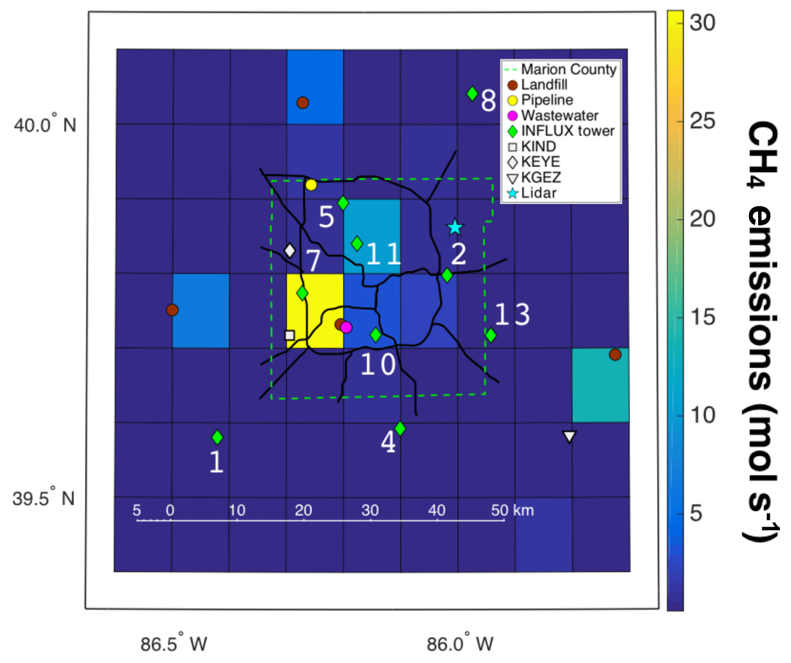
Figure 2 Map of the primary roads in Indianapolis, INFLUX towers, lidar system, weather stations, and a few CH₄ point sources plotted over the gridded CH₄ emissions (mol s⁻¹) from the EPA 2012 inventory (Maasakkers et al., 2016). The gridded map of emissions includes emissions from the mentioned point sources; their position is provided to aid in interpretation of the observations. The dashed bright green line denotes Marion County borders.

2.2 INFLUX tower network

The continuous GHG measurements from INFLUX are described in detail in Richardson et al. (2017). The measurements were made using wavelength-scanned cavity ring down spectrometers (CRDSs, Picarro, Inc., models G2301, G2302, G2401, and G1301), installed at the base of existing communications towers, with sampling tubes secured as high as possible on each tower (39–136 m above ground level (a.g.l.); Miles et al., 2017a). A few towers also included measurements at 10 m a.g.l. and one or two intermediate levels. While INFLUX tower in situ measurements began in September 2010, here we focus on the CH₄ measurements from 2013–2016. From June through December 2012, there were two or three towers with operational CH₄ measurements. By July 2013, five towers included measurements of CH₄, and throughout the majority of the years 2015–2016 there were eight INFLUX towers with CH₄ measurements (Fig. 3). Comparisons between flask and in situ measurements and round-robin-style testing indicated compatibility across the tower network of 0.6 ppb CH₄ (Richardson et al., 2017). In this study we use hourly means of CH₄.

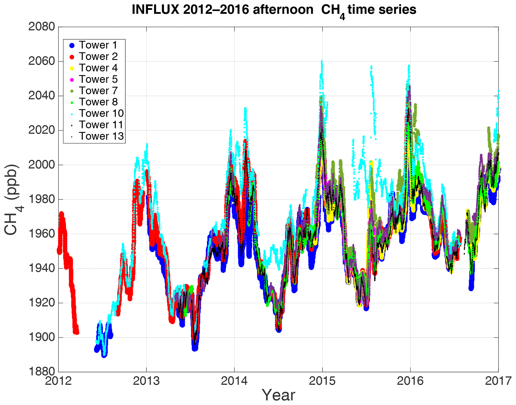
Figure 3 The 20 d running average of afternoon (12:00–16:00 LST; the hours are inclusive) CH₄ mole fractions as measured by the INFLUX tower network (highest available height is used) from 2012 through 2016.

2.3 Meteorological data

Wind speed and direction were measured at the Indianapolis International Airport (KIND), Eagle Creek Airpark (KEYE), and Shelbyville Municipal Airport (KGEZ). The data used are hourly values from the Integrated Surface Dataset (ISD) (https://www.ncdc.noaa.gov/isd, last access: 8 April 2020) and 5 min values directly from the Automated Surface Observing System (ASOS). A complete description of ASOS stations is available at https://www.weather.gov/media/asos/aum-toc.pdf (last access: 8 April 2020). The accuracy of the wind speed measurements are ±1 m s⁻¹ or 5 % (whichever is greater) and the accuracy of the wind direction is 5^∘ when the wind speed is ≥2.6 m s⁻¹. The anemometers are located at about 10 m a.g.l. The wind data reported in ISD are given for a single point in time recorded within the last 10 min of an hour and are closest to the value at the top of the hour.

The planetary boundary layer height (BLH) was determined from a Doppler lidar deployed in Lawrence, Indiana, about 15 km to the northeast of downtown. The lidar is a Halo Streamline unit, which was upgraded to have extended range capabilities in January 2016. The lidar continuously performs a sequence of conical, vertical-slice, and staring scans to measure profiles of the mean wind, turbulence, and relative aerosol backscatter. All of these measurements are combined using a fuzzy-logic technique to automatically determine the BLH continuously every 20 min (Bonin et al., 2018). The BLH is primarily determined from the turbulence measurements, but the wind and aerosol profiles are also used to refine the BLH estimate. The BLHs are assigned quality-control flags that can be used to identify times when the determined BLH is unreliable, such as when the air is exceptionally clean, the BLH is below a minimum detectable height, or clouds and fog that attenuate the lidar signal exist. Additional details about the algorithm and the lidar operation for INFLUX are provided in Bonin et al. (2018). Doppler lidar measurements are available at https://www.esrl.noaa.gov/csd/projects/influx/ (last access: 8 April 2020).

2.4 Urban methane background

Both the aircraft mass balance and inverse modeling methodologies rely on an accurate estimation of the urban CH₄ enhancement relative to the urban CH₄ background in order to produce a reliable flux estimate (Cambaliza et al., 2014; Lamb et al., 2016). The CH₄ mole fraction enhancement is defined as

$$\begin{array}{}\text{(1)}& C_{\mathrm{enhancement}}=C_{\mathrm{downwind}}-C_{\mathrm{bg}},\end{array}$$

where C_downwind is the CH₄ mole fraction measured downwind of a source and C_bg is the CH₄ background mole fraction, which can be measured upwind of the source, but this is not necessary. Background, as defined in this body of literature, is a mole fraction measurement that does not contain the influence of the source of interest, but which is assumed to accurately represent mole fractions that are upwind of the source of interest and measured simultaneously with the downwind mole fractions.

The aircraft mass balance studies of Indianapolis mentioned used two main methods to determine a background value. The first method calculates an average of the aircraft transect edges that lie outside of the city domain (Cambaliza et al., 2014). In the second approach, a horizontally varying background is introduced by linearly interpolating median background values of each of the transect edges (Heimburger et al., 2017). In theory there is also a third method that uses an upwind transect as a background field, but in the studies above it was assumed that the edges are representative of an upwind flow. In the case of an inversion, it is common to pick a tower that is located away from urban sources and has on average the smallest overall enhancement (Lauvaux et al., 2016). Because choosing the background involves a degree of subjectivity (Heimburger et al., 2017) we consider how these choices may influence emission estimates and introduce error, both random and systematic, using data from the INFLUX tower network.

Using tower network data from November 2014 through the end of 2016, two CH₄ background fields are generated for the city of Indianapolis based on two different sets of criteria. The notion is based on the fact that a choice of background is currently rather arbitrary in the literature (Heimburger et al., 2017), and at every point in time it is possible to choose multiple background values that are equally acceptable for the flux estimation. In our case both approaches identify a tower suitable to serve as a background for each of the eight wind directions (N, NE, E, SE, S, SW, W, NW), where an arc of 45^∘ represents a direction (e.g., winds from N are between 337.5 and 22.5^∘). Estimating background for different wind directions is implemented to more accurately represent upwind flow that is hopefully not contaminated by local sources.

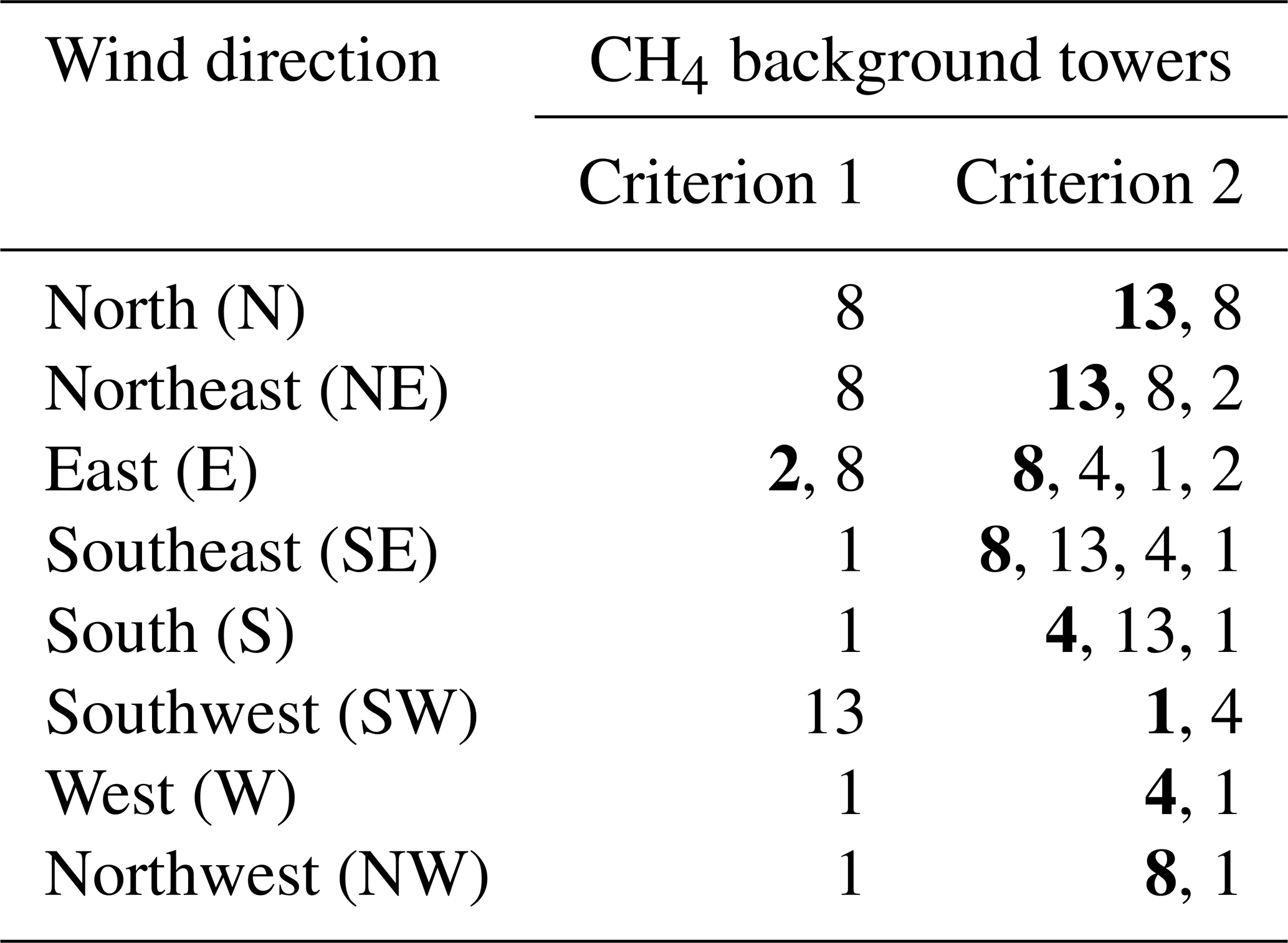
Criterion 1 corresponds to a typical choice of a background in a case of tower inversion and is based on the concept that the lowest CH₄ mole fraction measured at any given time is not affected by the city sources and therefore is a viable approximation of the background CH₄ mole fractions outside of the city (Miles et al., 2017a; Lauvaux et al., 2016). Given this assumption, the tower with the lowest median of the CH₄ enhancement distribution (calculated by assuming the lowest measurement among all towers at a given hour as a background) for each of the wind directions over the November 2014 through December 2016 time period is chosen as a background site (Miles et al., 2017a). Criterion 2 requires that the tower is outside of Marion County (outside of the city boundaries) and is not downwind of any known regional CH₄ source (Fig. 2). For some wind directions, there are multiple towers that could qualify as a background; we pick towers in such a manner that they are different for each criterion given a wind direction in order to calculate the error associated with the use of different but acceptable backgrounds. The towers used for both criteria and for each of the eight wind directions are displayed in Table 1. Quantifying differences between these two backgrounds allows for an opportunity to better understand the degree of uncertainty that exists in the atmospheric CH₄ background at Indianapolis.

Table 1 INFLUX towers used to estimate CH₄ background based on two different criteria. Numbers in bold indicate towers chosen to generate a background field when multiple options are possible (for more details see discussion). In short, criterion 1 uses towers with the lowest mean CH₄ for a specific wind direction, and criterion 2 uses towers outside of Marion County and not downwind of large sources (including the city as a whole).

To make the comparison as uniform as possible only data from 12:00–16:00 LST are utilized (all hours are inclusive) when the boundary layer is typically well mixed (Bakwin et al., 1998). A lag 1 autocorrelation is found between 12:00 and 16:00 LST; i.e., the hourly afternoon data are correlated to the next hour, but the correlation is not significant for samples separated by 2 h or more. Therefore, hours 13:00 and 15:00 LST are eliminated to satisfy the independence assumption for hourly samples. Furthermore, we make an assumption that the data satisfy steady-state conditions. If the difference between consecutive hourly wind directions exceeds 30^∘ or the difference between hours 16:00 and 12:00 LST exceeds 40^∘, the day is eliminated. Days with average wind speeds below 2 m s⁻¹ are also eliminated due to slow transport across the city (the transit time from tower 1 to tower 8 is about 7 h at a wind speed of 2 m s⁻¹).

2.5 Frequency and bivariate polar plots

Frequency and bivariate polar plots are used in this work to gain more knowledge regarding CH₄ background variability based on criteria 1 and 2, and to identify sources located within the city. To generate these polar plots, we use the openair package (from R programming language) created specifically for air quality data analysis (Carslaw and Ropkins, 2012). Bivariate and frequency polar plots indicate the variability of a pollutant concentration at a receptor (such as an observational tower) as a function of wind speed and wind direction, preferably measured at the location of the receptor or within several kilometers of the receptor. The frequency polar plot is generated by partitioning the CH₄ hourly data into the wind speed and direction bins of 1 m s⁻¹ and 10^∘ respectively. To generate bivariate polar plots, wind components u and v are calculated for hourly CH₄ mole fraction values, which are fitted to a surface using a generalized additive model (GAM) framework in the following way:

$$\begin{array}{}\text{(2)}& \sqrt{C}=\mathit{\beta }+s\left(u,v\right)+\mathit{ϵ},\end{array}$$

where C is the CH₄ mole fraction transformed by a square root to improve model diagnostics such as a distribution of residuals, β is mean of the response, s is the isotropic smoothing function of the wind components u and v, and ϵ is the residual. For more details on the model see Carslaw and Beevers (2013).

2.6 Temporal variability and approximate flux estimation

Temporal variability in urban CH₄ emissions may play an important role in the corresponding emissions quantification procedures. Lamb et al. (2016) suggested that such temporal variability might partially explain the differences among CH₄ flux estimates shown in Fig. 1. If temporal variability of CH₄ emissions exists within the city, disagreements in the CH₄ flux between studies could be attributed to differences in their sampling period. Because the INFLUX tower data at Indianapolis contain measurements at all hours of the day over multiple years, we can utilize this dataset to better understand the temporal variability in methane emissions in the city.

We apply a simplified atmospheric boundary layer budget, not to estimate precisely the actual city emissions, but rather to evaluate temporal variability of the emissions. We begin by assuming CH₄ emissions Q_a (mass per unit time per unit area) are not chemically active and are constant over a distance Δx spanning a significant portion of the city. The next assumption is that a CH₄ plume measured downwind of the city is well mixed within a layer of depth H (which is the same as BLH). We treat wind speed u as constant within the layer for every hour considered. Given the abovementioned assumptions we can write a continuity equation describing mass conservation of CH₄ concentration C within a box in the following fashion:

$$\begin{array}{}\text{(3)}& \mathrm{\Delta }xH{\displaystyle \frac{\partial C}{\partial t}}=\mathrm{\Delta }x{Q}_{\mathrm{a}}+uH\left(C_{\mathrm{b}}-C\right)+\mathrm{\Delta }x{\displaystyle \frac{\partial H}{\partial t}}\left(C_{\mathrm{a}}-C\right),\end{array}$$

where C_b is the CH₄ concentration upwind of the city (or background), and C_a is the CH₄ concentration above the mixed layer (Hanna et al., 1982; Arya, 1999; Hiller et al., 2014). The left-hand side of the equation represents the change in CH₄ concentration with time, ΔxQ_a denotes a constant CH₄ source over the distance Δx, uH(C_b−C) indicates a change of CH₄ concentration due to horizontal advection, and finally the $\mathrm{\Delta }x\frac{\partial H}{\partial t}\left(C_{\mathrm{a}}-C\right)$ term accounts for the vertical advection and encroachment processes that result from changing BLH. By assuming steady-state conditions ($\frac{\partial C}{\partial t}=\mathrm{0}$ and $\frac{\partial H}{\partial t}=\mathrm{0})$, the equation can be simplified to

$$\begin{array}{}\text{(4)}& Q_{\mathrm{a}}={\displaystyle \frac{uH\left(C-C_{\mathrm{b}}\right)}{\mathrm{\Delta }x}}.\end{array}$$

We use Eq. (4) to estimate hourly CH₄ emissions (Q_a) from Indianapolis (see assumptions in the paragraph below) given hourly averaged data of H from the lidar positioned in the city, wind speed (u) from the local weather stations, and upwind (C_b) and downwind (C) CH₄ mole fractions measured (and then converted to concentrations) at towers 1, 8, and 13 (depending on a wind direction) using data from heights of 40, 41, and 87 m respectively (see Fig. 2).

The CH₄ concentrations are derived from CH₄ mole fractions by approximating average molar density of dry air (in mol m⁻³) within the boundary layer for every hour of the day, where variability of pressure with altitude is calculated using the barometric formula, and it is assumed that temperature decreases with altitude by 6.5 K per kilometer. The hourly surface data for pressure and temperature are taken from KIND weather station. The difference between concentrations C and C_b is instantaneous and not lagged, where C_b represents an air parcel entering the city and C represents the same air parcel exiting the city (Turnbull et al., 2015). The CH₄ enhancements (C−C_b) are estimated for daytime by averaging observations spanning 12:00–16:00 LST and for nighttime by averaging observations spanning 20:00–05:00 LST. These time periods are based on lidar estimations of when on average H varies the least. Each daytime and nighttime were required to contain at least 3 and 9 h of CH₄ values respectively for averaging to occur, otherwise they were eliminated from the computation process. Observations when H is below 100 m are not used to avoid the cases when measurements from towers may be above the boundary layer. In order to better achieve the assumption that the boundary layer is fully mixed (especially at night), all hours with wind speeds below 4 m s⁻¹ are eliminated (Van De Wiel et al., 2012). To approximate the emissions of the whole city we need to know the approximate area of the city and the distance over which the plume is affected by the city CH₄ sources. The area of the city is about 1024 km² (the area of Marion County) and the length that plume traverses when it is over the city ranges from 32 to 35 km depending on which downwind tower is used. We assume that CH₄ measurements at towers 8 and 13 are representative of a vertically well-mixed city plume as the towers are located outside of the city boundaries and allow for sufficient vertical mixing to occur. For S and SW wind directions tower 8 observations are used to represent downwind conditions, with background observations coming from towers 1 and 13, respectively (based on criterion 1 shown in Table 1). For W wind direction, tower 13 observations represent the downwind with background obtained from tower 1. The wind direction is required to be sustained for at least 2 h, otherwise the data point is eliminated.

2.7 Indianapolis CH₄ sources

Only a few known CH₄ point sources exist within Indianapolis (Cambaliza et al., 2015; Lamb et al., 2016). The South Side landfill (SSLF), located near the center of the city, is thought to be the largest point source in the city, with emissions ranging between about 28 mol s⁻¹ (inventory from Maasakkers et al., 2016, GHG reporting program, and inverse estimates from ground-based mobile sampling employed in Lamb et al., 2016) and 45 mol s⁻¹ (aircraft; Cambaliza et al., 2015) depending on an emission estimation methodology. However, using Cambaliza et al. (2015) aircraft data and applying a different background formulation, Lamb et al. (2016) found emission values of SSLF closely agreeing with the 28 mol s⁻¹ estimate. SSLF could account for as little as 33 % (top-down from Cambaliza et al., 2015) or as much as 63 % (inventory from Maasakkers et al., 2016) of total Marion County CH₄ emissions. Other city point sources are comparatively small; the wastewater treatment facility located near SSLF contributes about 3–7 mol s⁻¹ (inventory from Lamb et al., 2016), and the transmission–distribution transfer station at the Panhandle Eastern Pipeline (also known as a city gate and in this study abbreviated to PEP) is estimated to be about 1 mol s⁻¹ (inventory from Lamb et al., 2016). The remaining CH₄ sources, mainly from NG infrastructure leaks and livestock, are considered to be diffuse sources and are not well known. Potential sources of emissions related to NG activities include gas regulation meters, transmission and storage, distribution leaks, and compressed natural gas (CNG) fleets. These diffuse NG sources account for 21 %–67 % of the city emissions or 20 mol s⁻¹ (inventory from Maasakkers et al., 2016) to 64 mol s⁻¹ (top-down from Cambaliza et al., 2015). Livestock emissions for Marion County are estimated to be around 1.5 mol s⁻¹ (inventory from Maasakkers et al., 2016). These prior studies present conflicting conclusions regarding the magnitude of the diffuse NG CH₄ source in Indianapolis.

3 Results and discussion

3.1 Inversion and city boundaries

A significant portion of CH₄ emissions across the US can be characterized by numerous relatively large point sources scattered throughout the country rather than by broad areas of smaller enhancements (Maasakkers et al., 2016). Because of this, the total emissions for a given domain can be very sensitive to how that domain is defined. A small increase or decrease in the domain area could add or remove a large point source and significantly impact the total emissions defined within the domain.

In the case of Indianapolis, this issue became apparent when the emissions were calculated using an atmospheric inversion model (Lamb et al., 2016; Lauvaux et al., 2016). The atmospheric inversion solved for fluxes in domain 1 (Fig. 2), which significantly increased the estimated emissions in comparison with the inventory values that were gathered mainly within Marion County (domain 2). When reduced to domain 2, the inverse modeling emission estimate decreases to 107 mol s⁻¹ (from about 160 mol s⁻¹), which falls within an error bar of the Lamb et al. (2016) inventory estimate. This difference is significant and could at least partially explain the discrepancy shown in Fig. 1 between the emission values from the inventories and emission results from the inverse modeling. However, even the decreased inverse modeling estimate is about 91 % higher than the inventories.

Additionally, the subject of the domain is relevant for airborne mass balance flights because a priori the magnitude and variability of background plume is unknown and could be easily influenced by upwind sources. The issue of background is discussed further in the next section.

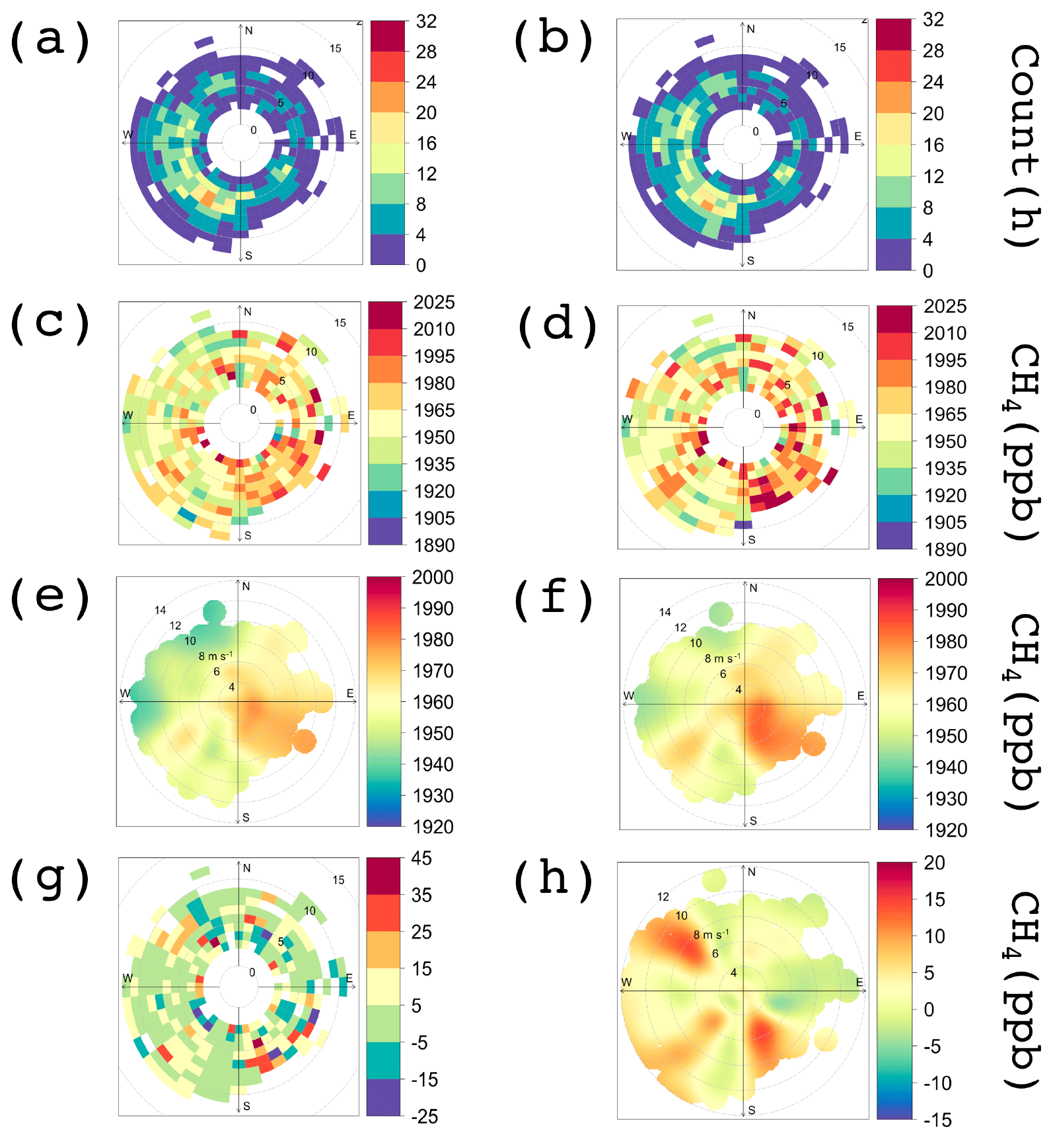
Figure 4 Frequency and bivariate polar plots of CH₄ background for Indianapolis using data from 12:00–16:00 LST, November 2014 through December 2016 given two different criteria (Table 1). (a) Polar histogram indicating a number of hourly measurements available using criterion 1. (b) Same as (a) only for criterion 2. Differences between (a) and (b) are due to slight differences in data availability at the considered towers. (c) Polar frequency plot of the CH₄ background using criterion 1. (d) Same as (c) only for criterion 2. (e) Polar bivariate plot of CH₄ background using criterion 1. (f) Same as (e) only for criterion 2. (g) Polar frequency plot of difference between the backgrounds: criterion 2 − criterion 1. (h) Same as (g) but shown with a bivariate polar plot.

3.2 Variability in CH₄ background

Comparisons between criterion 1 and criterion 2 CH₄ background mole fractions as a function of wind speed and direction are visualized using frequency and bivariate polar plots (Fig. 4). Both backgrounds generally agree on the higher CH₄ originating from the SW, SE, and E wind directions (Fig. 4c–f); however, the values themselves differ, especially when winds are from NW, SW, and SE. As background difference plots (Fig. 4g–h) indicate, there is a noticeable variability between the magnitudes of the CH₄ backgrounds, where criterion 2, by design, typically has higher background mole fractions. The background differences, at a given hour, suggest that the CH₄ field flowing into the city is heterogeneous, with differences between towers ranging from 0 to over 45 ppb (Fig. 4g). Because large gradients in CH₄ background over the city could pose challenges for flux estimations using top-down methods such as inverse modeling and aircraft mass balance, it is imperative to establish whether the background differences vary randomly or systematically and how to choose a background to minimize these errors.

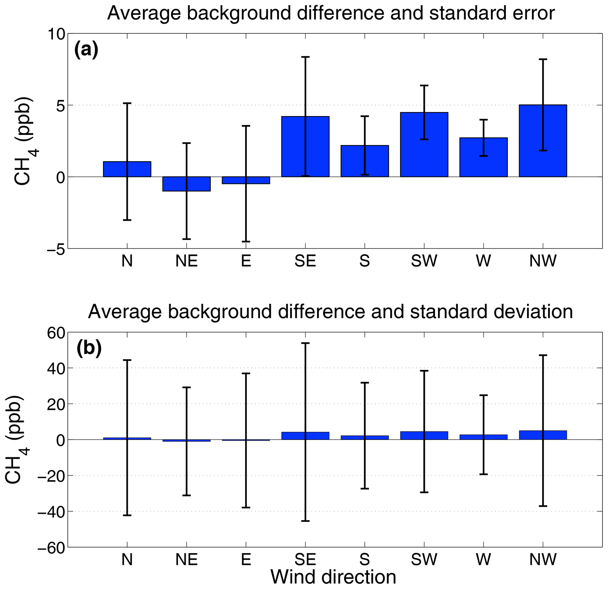
Figure 5 Average of the differences between criteria 2 and 1 CH₄ backgrounds at Indianapolis as a function of wind direction. These averages are generated from the same data that are used in Fig. 4 and reflect results shown in Fig. 4g. Error bars indicate in (a) 2 times the standard error and in (b) 2 times the standard deviation.

To further understand the nature of background variability we calculate the mean, standard deviation, and standard error of background hourly differences between criterion 2 and criterion 1 from November 2014 to December 2016 for each of the eight wind directions mentioned in Table 1. The results are shown in Fig. 5. Systematic bias is evident for the SE, S, SW, W, and NW wind sectors, whereas random error dominates the N, NE, and E wind directions. Wind directions showing statistically significant bias have mean biases ranging from 2 to 5 ppb, with values as large as 8 ppb falling within the range of 2 times the standard error. The standard deviation plot indicates a potential background discrepancy that can occur on any given day, where the W wind direction is the least variable, with 2 times the standard deviation close to 20 ppb, while SE wind direction is the most variable, with 2 times the standard deviation falling at about 50 ppb.

Random errors in the mole fractions of background differences (biases) are also important and are a function of the length of the data record. We quantify the random error in the CH₄ background mole fraction differences using the bootstrap method by randomly sampling 2 to 150 h (small and large sample size) of the background CH₄ differences for each of the wind directions with replacements (we make the assumption that our differences are independent since we eliminated lag 1 autocorrelation from the data). This sub-sampling experiment is repeated 5000 times (Efron and Tibshirani, 1986). The standard deviations of the mean (standard error) of the 5000 simulated differences are calculated for each wind direction. The resulting standard errors of the city CH₄ background differences, multiplied by 2 to represent the 95 % confidence intervals, are shown as a function of the length of the data record in Fig. 6. Because random error falls as sample size grows it makes sense to assign a threshold indicating a minimum number of samples needed to achieve a theoretical precision for each wind direction.

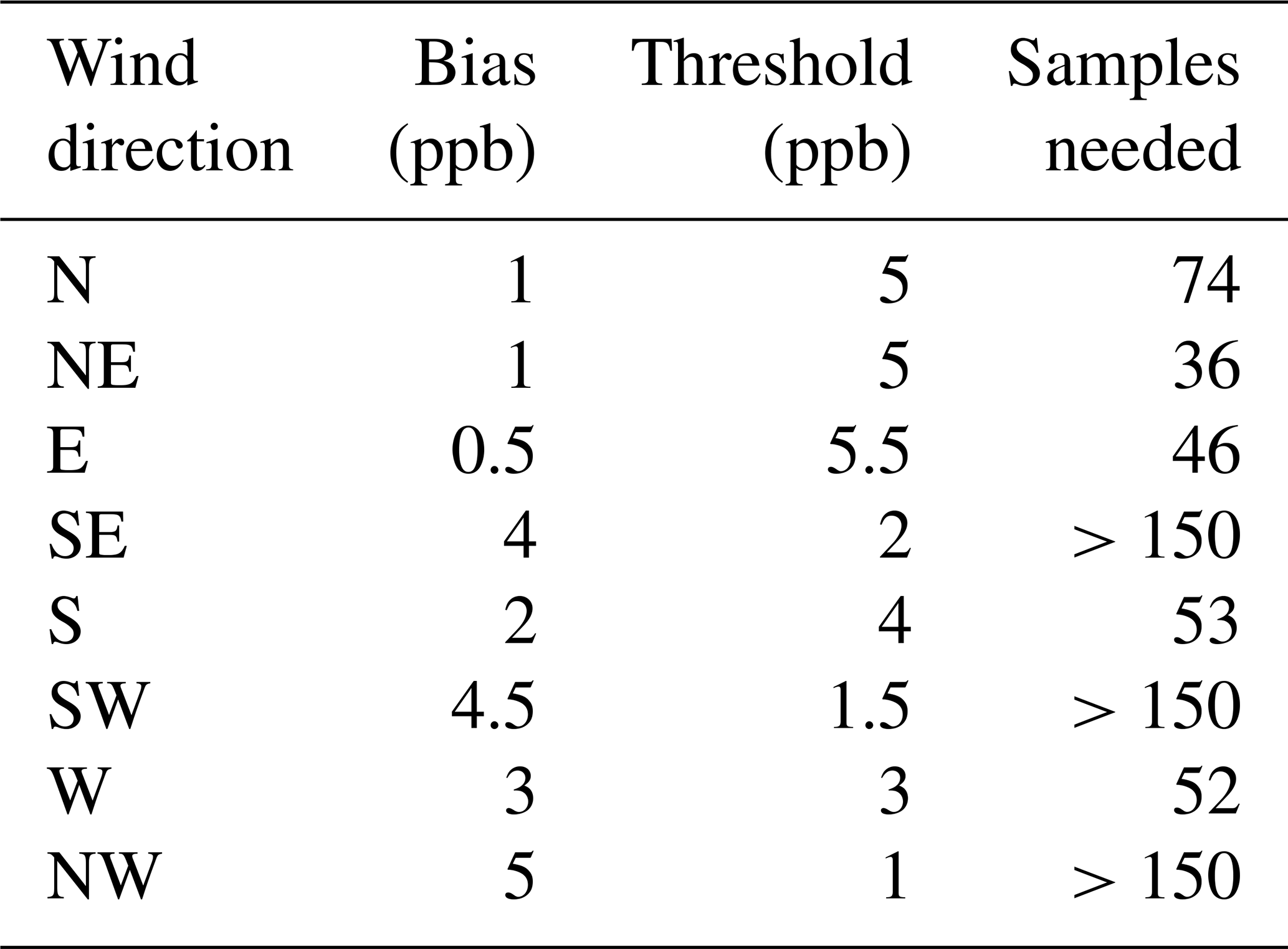
One way to assign a required precision would be to make sure that the standard error (random error) reaches a point where it is less than the Indianapolis enhancement of about 12 ppb (a higher estimate of the Indianapolis enhancement from Sect. 3.3) by a factor of 2 when combined with a bias (Table 2), meaning that the sum of bias and standard error must be at most 6 ppb. In this approach each wind direction would have a different threshold because of the differences in biases. For instance, given this requirement the NW direction would need a random error of 1 ppb since its bias is 5 ppb. For the NW direction, this threshold would require more than 150 samples. For the N direction on the other hand, where the bias is 1 ppb, the requirement is fulfilled when random error crosses 5 ppb at 74 samples. Now we consider these random and systematic errors in CH₄ background differences in the context of Indianapolis urban CH₄ emissions.

Figure 6 Bootstrap simulation of two times the standard error in Indianapolis CH₄ background mole fraction differences (between criteria 2 and 1) as a function of sample size and wind direction (see text for details). Thresholds for each of the wind directions indicate a random error threshold needed for the background uncertainty to be within 50 % of Indianapolis CH₄ enhancement of 12 ppb.

Table 2 A number of independent samples needed (column 4) to satisfy the combined requirement of 6 ppb background error based on the sum of bias and random error (explained in Sect. 3.2) as a function of wind direction.

For Indianapolis, using the INFLUX network, we estimated that depending on sample size (number of hours sampled) and wind direction, background gradient across the city over 12:00–16:00 LST could vary from 0 to about 50 ppb (Fig. 5b). Given that the average afternoon CH₄ enhancement of the city is around 8–12 ppb (Sect. 3.3; Fig. 7; Cambaliza et al., 2015; Miles et al., 2017a), the error on the estimated emissions could easily be over 100 % if the analysis does not approach the issue of background with enough sampling. A sample size of about 50 independent hours significantly decreases background uncertainty for N, NE, E, S, and W wind directions and allows for a more accurate assessment of the CH₄ emissions at Indianapolis. For CH₄ sources with a significantly larger signal than their regional background, the mentioned background variability becomes less impactful on results, but because Indianapolis is a relatively small emitter of CH₄, and because there are relatively large sources outside of the city, uncertainties due to background estimation are comparatively large. Our uncertainty assessment suggests that the highly variable CH₄ emission values of Indianapolis from aircraft mass balance calculations shown in Fig. 1 are at least partially due to the variability in the urban CH₄ background of Indianapolis.

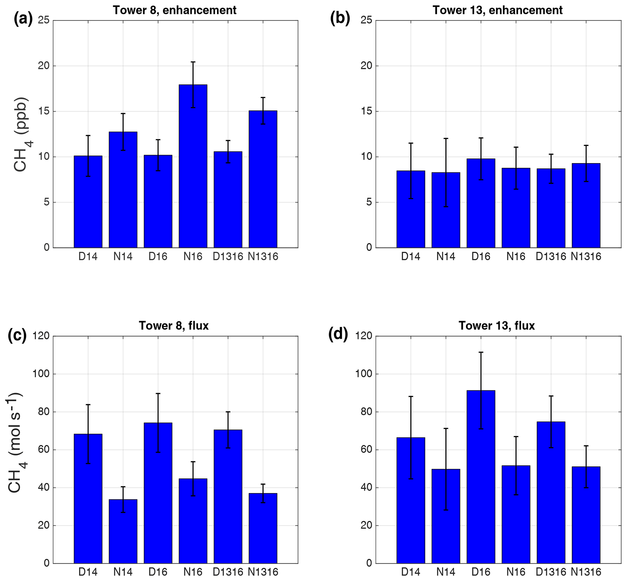
Figure 7 Averages of the daytime (D) and nighttime (N) CH₄ enhancements and fluxes at INFLUX towers 8 and 13 for years 2014 (14), 2016 (16), and 2013–2016 (1316). The error bars represent the 95 % confidence interval of each mean value. (a) Estimates of CH₄ enhancements from tower 8. (b) Estimates of CH₄ enhancements from tower 13. (c) Estimates of CH₄ flux from tower 8. (d) Estimates of CH₄ flux from tower 13.

3.3 Temporal variability of methane enhancements and fluxes in Indianapolis

Figure 7 presents average CH₄ mole fraction enhancements and flux calculations (Eq. 4) at towers 8 and 13 for years 2014, 2016, and 2013–2016 (for the detailed methodology see Sect. 2.6). The years of 2014 and 2016 are chosen for temporal comparison because they do not contain major BLH data gaps. The error bars in the figure show the standard error multiplied by 2 indicating 95 % confidence interval of each average.

One of the more interesting features in Fig. 7 is a day–night variability of CH₄ emissions at Indianapolis. The most prominent example of this feature is found in Fig. 7c, where the estimates for both years suggest that daytime emissions are approximately twice as large as the emissions at night. The decrease in the CH₄ emissions at night also appears in tower 13, but the errors are too high in those estimates to make any definitive conclusions. A similar urban CH₄ emissions diurnal variability is reported by Helfter et al. (2016) in their study of GHGs for London, UK, where they attribute diurnal variation of CH₄ emissions to the NG distribution network activities, fugitive emissions from NG appliances, and temperature-sensitive CH₄ emission sources of biogenic origin (such as a landfill). Taylor et al. (2018) suggest that CH₄ emissions from landfills exhibit a diurnal cycle with higher emissions in the early afternoon and 30 %–40 % lower emissions at night.

With regard to yearly temporal variability we are only able to compare years 2014 and 2016 due to limited BLH data for other years. Results from both towers suggest that Indianapolis overall CH₄ emissions did not change significantly between 2014 and 2016. Although it is important to be cautious about interpreting actual flux estimations given the assumptions mentioned in Sect. 2.6, it is interesting to note that the flux values from both towers average to about 70 mol s⁻¹, which puts our value right in between inventory and inversion estimates shown in Fig. 1. If we assume that SSLF emissions are generally known (GHG reporting program) that would indicate that emissions from NG distribution are likely to be about 14 mol s⁻¹ (70 %) higher than what both of the inventories currently estimate but within the error bars of the Lamb et al. (2016) inventory calculation. Another possible scenario is that SSLF emissions are higher than what is currently assumed. Given these complexities, uncertainty regarding the exact emissions from NG distribution at Indianapolis still remains.

3.4 Methane sources in Indianapolis

Bottom-up emission inventories have difficulty tracking changes in sources over time. Our continuous tower network observations can monitor temporal and spatial variability in sources of CH₄ in Indianapolis. To do so we employ the aforementioned bivariate polar plots to verify known sources and potentially identify unknown sources across the city. We compare two time periods, 2014–2015 (two full years) and 2016. Figure 8 displays bivariate polar plots of CH₄ enhancements using criterion 1 background at 9 INFLUX towers in Indianapolis over the two years of 2014 and 2015. Figure 9 shows the same plot, but for the year 2016. Here we have separated 2016 from 2014–2015 because of different results noted during these times.

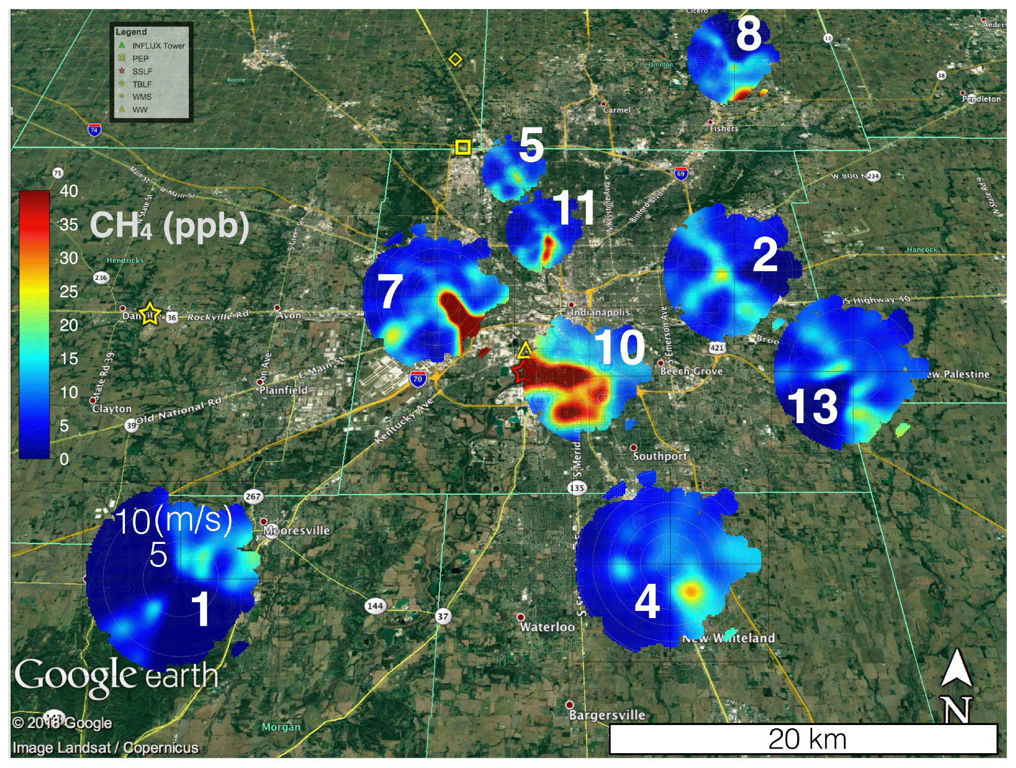
Figure 8 © Google Earth image overlaid with bivariate polar plots (Sect. 2.5) of the CH₄ enhancements at nine INFLUX towers in Indianapolis using the criterion 1 background (Table 1) for the full years of 2014 and 2015 over the afternoon (12:00–16:00 LST). The wind speed scale is only labeled at site 1; other sites follow the same convention. The legend indicates known sources of CH₄: Panhandle Eastern Pipe Line (PEP), South Side landfill (SSLF), Twin Bridges landfill (TBLF), Waste Management Solutions (WMS), and a wastewater treatment facility (WW). The known magnitudes of sources that are in Marion County (PEP, SSLF, and WW) are reported in Sect. 2.7. Magnitudes of TBLF and WMS according to EPA are approximately 5 mol s⁻¹. The largest known source on the map is SSLF.

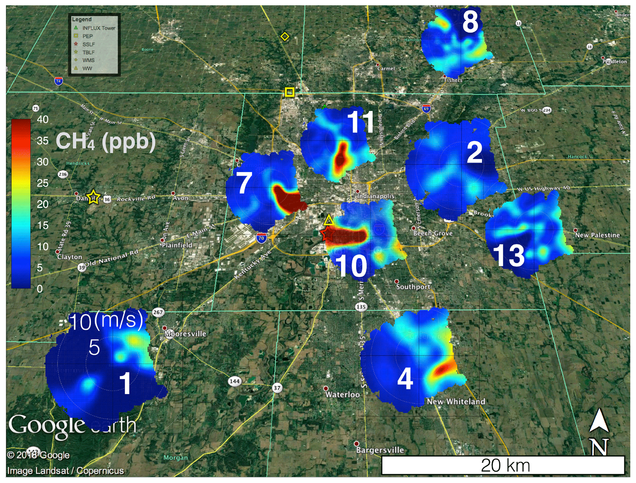
Figure 9 © Google Earth image overlaid with bivariate polar plots (Sect. 2.5) of the CH₄ enhancements at nine INFLUX towers in Indianapolis using the criterion 1 background (Table 1) for the year 2016 over the afternoon (12:00–16:00 LST). The wind speed scale is only labeled at site 1; other sites follow the same convention. The legend indicates known sources of CH₄: Panhandle Eastern Pipe Line (PEP), South Side landfill (SSLF), Twin Bridges landfill (TBLF), Waste Management Solutions (WMS), and a wastewater treatment facility (WW). The known magnitudes of sources that are in Marion County (PEP, SSLF, and WW) are reported in Sect. 2.7. Magnitudes of TBLF and WMS according to EPA are approximately 5 mol s⁻¹. The largest known source on the map is SSLF.

The images reveal that the most consistent and strongest source in the city is the SSLF. This is most evident from the 40+ ppb CH₄ enhancements detected at towers 7, 10, and 11 coming from the location of the SSLF (by triangulation). Enhancements from the landfill appear to also be detectable at towers 2, 4, 5, and 13. Based on these observations it can be concluded that there are no other point sources in Marion County comparable in size to the SSLF. A small fraction of the SSLF plume is likely due to the co-located wastewater facility, but the inventory estimates suggest that the wastewater treatment facility is responsible for no more than 7 % of this plume (Cambaliza et al., 2015; Maasakkers et al., 2016). The PEP, located in the northwestern section of the city, may be partially responsible for a plume of 5–10 ppb at towers 5 and 11. However, the plume is less detectable using the criterion 2 background value that has higher background (using tower 8 as a background) from the NW wind direction (not shown), adding uncertainty to the true magnitude of the enhancement from this source. The same is true for towers 2 and 13, which have pronounced plumes when winds are from the NW with the criterion 1 background, but when background 2 is used these plumes vanish (not shown). Such inconsistency makes it difficult to attribute these plumes to a specific source.

Another important point is the cluster of large enhancements surrounding tower 10 in 2014–2015. Because no other tower sees these enhancements (at least at comparable magnitudes), we believe that they are the result of nearby NG leaks. These plumes are not consistent temporally or spatially as they mostly disappear in 2016, potentially indicating that they are transient and localized NG distribution leaks. It is difficult to ascertain the exact combined magnitude of these leaks since they mix together with SSLF into an aggregated city plume when observed from downwind towers such as 8 and 13. None of the individual leaks appears to be similar in magnitude to the emissions that originate from SSLF. Diffuse NG emissions comparable to the SSLF source (Lamb et al., 2016) may exist. Our flux estimations at towers 8 and 13, however, imply that the magnitude of the NG diffuse source suggested by the top-down analyses in Cambaliza et al. (2015) and Lamb et al. (2016) are probably overestimates (see Sect. 3.3). We hypothesize that the relatively high Indianapolis CH₄ emissions (see Fig. 1) reported by Cambaliza et al. (2015) could be a result of random errors in upwind conditions (see Sect. 3.2) influencing the small number of airborne flux estimates.

4 Conclusions

We have examined four potential contributions to discrepancies between urban top-down and bottom-up estimates of CH₄ emissions from Indianapolis: domain definition, heterogeneous background mole fractions, temporal variability in emissions, and sources missing from inventories. Results indicate that the urban domain definition is crucial for the comparison of the emission estimates among various methods. Our atmospheric inverse flux estimates for Marion County, which is similar to the domain that is analyzed by inventory and airborne mass balance methodologies (Mays et al., 2009; Cambaliza et al., 2014; Lamb et al., 2016), is 107 mol s⁻¹ compared to the 160 mol s⁻¹ that is estimated for the larger domain (Hestia inventory domain; Gurney et al., 2012). This partially explains higher emissions in inverse modeling estimates shown by Lamb et al. (2016); however, 107 mol s⁻¹ is still 91 % higher than what EPA and Lamb et al. (2016) find in their inventories (Fig. 1).

To better understand background variability at Indianapolis two different but acceptable background estimates, based on specific criteria for each wind direction, and their differences are used to assess the heterogeneity of the CH₄ background at Indianapolis. Background criterion 1 looks for a tower that is consistently lower than other towers, while background criterion 2 picks a tower that is outside of Marion County domain and is not downwind of any nearby sources as determined by the EPA 2012 inventory. We focus on midday atmospheric conditions to avoid the complexities of vertical stratification in the stable boundary layer. The midday Indianapolis atmospheric CH₄ mole fraction background is shown to be heterogeneous, with 2–5 ppb statistically significant biases for the NW, W, SW, S, and SE wind directions. Random errors of background differences are a function of sample size and decrease as a number of independent samples increase. Small sample sizes, such as a few hours of data from a single point, are prone to random errors on the order of 10–30 ppb in the CH₄ background, similar to the magnitude of the total enhancement from the city of Indianapolis, which is estimated to be on average around 10–12 ppb. Longer-term sampling and/or more extensive background sampling are necessary to reduce the random errors. Sample size required to reduce random errors of background differences to an acceptable value for flux calculation is largely dependent on a wind direction. Both bias (long-term average of background differences) and its random error are important when estimating total background uncertainty. The results indicate that the N, NE, E, S, and W wind directions are more favorable for flux estimation and would require multiple days of measurements (e.g., about 50 independent hours of measurements) to reduce background uncertainty to about 6 ppb, which is half the magnitude of the typical CH₄ enhancement from Indianapolis. The remaining wind directions would require over 150 independent hourly measurements to achieve similar precision. We also estimate that depending on a wind direction for any given hour the spatial variability in background can be anywhere from 0 to 50 ppb. This uncertainty in the CH₄ background may partially explain the Heimburger et al. (2017) finding of large variability in airborne estimates of Indianapolis CH₄ emissions. Given many samples, the airborne studies converge to an average value of CH₄ flux that is noticeably closer to the inventory estimates for Indianapolis than several of the individual estimates presented in Fig. 1.

Measurement and analysis strategies can minimize the impacts of these sources of error. Spatially extensive measurement of upwind CH₄ mole fractions are recommended. For towers or other point-based measurements, multiple upwind measurement locations are clearly beneficial. For the aircraft mass balance approach, we recommend an upwind transect to be measured, lagged in time if possible, to provide a more complete understanding of the urban background conditions. Complex background conditions might suggest that data from certain days or wind directions should not be used for flux calculation. Finally, a mesoscale atmospheric modeling system informed with the locations of important upwind CH₄ sources can serve as a powerful complement to the atmospheric data (Barkley et al., 2017). Such simulations can guide sampling strategies and aid in interpretation of data collected with moderately complex background conditions.

With regard to temporal variability, no statistically detectable changes in the emission rates were observed when comparing 2014 and 2016 CH₄ emissions. However, a large difference between day and night CH₄ emissions was implied from a simple budget estimate. Night (20:00–05:00 LST) emissions may be 2 times lower than the emissions during the afternoon (12:00–16:00 LST) hours. Because prior estimates of top-down citywide emissions are derived using afternoon-only measurements, overall emissions of Indianapolis may be lower than these studies suggest. This bias may be present in studies performed in other cities as well. Our study suggests that day–night differences in CH₄ emissions must be understood if regional emission estimates are to be calculated correctly. Long-term, tower-based observations are an effective tool for understanding and quantifying multi-year variability in urban emissions.

One final point addressed in this study is the location of major CH₄ sources in Indianapolis. Analysis of the INFLUX tower observations suggest a diffuse NG source that exceeds both of the inventory estimates by 70 %, but additionally our analysis shows that the discrepancy is less than that proposed by the highest values reported in Lamb et al. (2016) (see Fig. 1). Uncertainty remains regarding the magnitude of the diffuse NG source of CH₄. The only major point source in the city is SSLF and it is observed at multiple towers. There is evidence for occasional point-source NG leaks, but they appear to be transient in time and limited in their strength.

Overall, assessment of the CH₄ emissions at Indianapolis highlights a number of uncertainties that need to be considered in any serious evaluation of urban CH₄ emissions. These uncertainties are amplified for Indianapolis since the enhancement signal from its CH₄ emissions is comparable in magnitude to variability in the regional background flow and as our results show it may be difficult at times to distinguish noise in the background from the actual city emissions signal. The evaluation of larger CH₄ sources may be easier with respect to separating signal from background. However, all of the points raised in this work will be nonetheless relevant and need to be addressed for our understanding of urban CH₄ emissions to significantly improve.