the Creative Commons Attribution 4.0 License.
the Creative Commons Attribution 4.0 License.
 | 11 Feb 2020
Characterization of the air–sea exchange mechanisms during a Mediterranean heavy precipitation event using realistic sea state modelling
Cindy Lebeaupin Brossier
Marie-Noëlle Bouin
Véronique Ducrocq
This study investigates the mechanisms acting at the air–sea interface during a heavy precipitation event that occurred between 12 and 14 October 2016 over the north-western Mediterranean area and led to large amounts of rainfall (up to 300 mm in 24 h) over the Hérault region (southern France). The study case was characterized by a very strong (>20 m s−1) easterly to south-easterly wind at low level that generated very rough seas (significant wave height of up to 6 m) along the French Riviera and the Gulf of Lion. In order to investigate the role of the waves on air–sea exchanges during such extreme events, a set of numerical experiments was designed using the Météo-France kilometre-scale AROME-France numerical weather prediction model – including the WASP (Wave-Age-dependant Stress Parametrization) sea surface turbulent flux parametrization – and the WaveWatch III wave model. Results from these sensitivity experiments in the forced or coupled modes showed that taking the waves generated by the model into account increases the surface roughness. Thus, the increase in the momentum flux induces a slowdown of the easterly low-level atmospheric flow and a displacement of the convergence line at sea. Despite strong winds and a young sea below the easterly flow, the turbulent heat fluxes upstream of the precipitating system are not significantly modified. The forecast of the heaviest precipitation is finally modified when the sea state is taken into account; notably, in terms of location, this modification is slightly larger in the forced mode than in the coupled mode, as the coupling interactively balances the wind sea, the stress and the wind.
- Article
(25134 KB) - Full-text XML
- BibTeX
- EndNote


The western Mediterranean region is regularly affected by heavy precipitation events (HPEs) that are characterized by a large amount of rainfall over a small area in a very short time; these events can lead to flash flooding, causing severe damage and, in some cases, casualties (e.g. Delrieu et al., 2005; Llasat et al., 2013). Usually such events are generated by quasi-stationary mesoscale convective systems (MCSs) that develop east of an upper-level trough and are enhanced by an unstable low-level jet advecting moist and warm air towards the Mediterranean coasts (Nuissier et al., 2011; Duffourg et al., 2016). Several mechanisms leading to the initiation of deep convection have been identified (Ducrocq et al., 2008, 2016); in particular, the forcing from mountainous coastal regions surrounding the Mediterranean Sea causes the unstable low-level flow to lift and, thus, triggers deep convection. Besides orographic lifting, deep convection can also be triggered by low-level wind convergence and cold pools due to precipitation evaporation.
The Mediterranean Sea, which is still warm in autumn, acts as a reservoir of moisture and heat that feeds the low-level flow by up to 40 %–60 %, according to the study by Duffourg and Ducrocq (2011) of 10 HPEs over south-western France. Therefore, air–sea exchanges during these episodes are key processes of such events. These exchanges, namely the sea surface turbulent heat, moisture and momentum fluxes, can be modulated by the sea surface conditions, including the temperature (SST), sea state and wind. Indeed, previous studies have shown that fluctuations in the SST can induce variations in the atmospheric low-level dynamics and stability as well as in precipitation (e.g. Lebeaupin Brossier et al., 2006; Cassola et al., 2016; Stocchi and Davolio, 2017; Meroni et al., 2018; Strajnar et al., 2019). How the sea surface turbulent fluxes are formulated in the models also has a significant impact on the rainfall amounts simulated during HPEs (Lebeaupin Brossier et al., 2008).
The momentum transfer from air to ocean strongly depends on the sea state. In the case of wind-generated waves, the wave-induced stress represents a large fraction of the total stress that causes an enhancement of the drag airflow and, therefore, modifies the wind profile and the near-surface dynamics (Janssen, 1989, 1991, 1992; Donelan, 1990). Analyses of in situ data highlighted the strong relationship between the sea surface roughness length (z0) and the wave age (Smith et al., 1992; Donelan et al., 1993; Drennan et al., 2003).
Nowadays, several bulk parameterizations of the sea surface turbulent fluxes include this relationship between z0 and the wave age. For example, the commonly used Coupled Ocean–Atmosphere Response Experiment (COARE) 3.0 sea surface turbulent parametrization (Fairall et al., 2003) enables one to consider the sea state in the momentum flux parametrization – using either the formulation from Oost et al. (2002) or that from Taylor and Yelland (2001) – via the relationship between z0 and the Charnock coefficient. Using the former formulation from Oost et al. (2002) in high-resolution numerical experiments of HPEs, Thévenot et al. (2016) and Bouin et al. (2017) showed an impact on the location of precipitation when the sea state forcing is taken into account in the sea surface turbulent flux parametrization. Nevertheless, these formulas are known to produce overly strong fluxes when strong winds (>20 m s−1) are encountered (Pineau-Guillou et al., 2018).
Besides directly controlling the momentum flux, surface roughness also impacts the turbulent heat fluxes and the turbulent structure and thickness of the atmospheric boundary layer (Doyle, 1995, 2002). For example, an impact on the thermodynamic structure and on the moisture transfer affecting the evolution of a convective system has recently been shown by Varlas et al. (2018) using an air–wave coupled system over the Mediterranean region.
In addition, under strong wind conditions, the intense breaking of ocean waves occurs and generates sea spray. This sea spray effect has a significant impact on the moisture and heat transfer at the air–sea interface that has been highlighted in several papers (e.g. Andreas, 1992; Andreas et al., 1995; Kepert et al., 1999; Bao et al., 2000, 2011; Bianco et al., 2011).
Based on this, recent studies have implemented different formulations in order to better account for the sea state and the sea spray effect on the sea surface roughness and heat and momentum fluxes during extreme events, such as Hurricane Arthur (Garg et al., 2018) or medicanes (Mediterranean tropical-like cyclones; Rizza et al., 2018). They showed that including the surface wave effects significantly improved the simulated track as well as the intensity and the maximum wind speed of the storm.
The sea state evolution can be retrieved from numerical wave model outputs and can then be used as a surface forcing in atmospheric models. However, coupled atmosphere–wave systems allow one to take the feedback of the modified wind profile to the wind–wave generation into account. Previous studies have demonstrated the importance of wind–wave coupling, showing significant effects on the representation of the atmospheric low-level dynamics (e.g. Janssen, 2004; Renault et al., 2012; Ricchi et al., 2016; Katsafados et al., 2016; Wahle et al., 2017; Varlas et al., 2018). They have also shown impacts on the drag coefficient over rough sea and on the momentum flux resulting in a reduced simulated surface wind speed. Moreover, all of these studies have clearly reaffirmed the need for a better representation of the sea state in the current understanding of air–sea exchanges. The present study investigates the impact of waves on a Mediterranean HPE using a kilometric-scale coupled atmosphere–wave system. The coupling involves the WaveWatch III wave model and the AROME numerical weather prediction model with a new flux parametrization (WASP) that uses explicit wave parameters to compute the wave age and, subsequently, the z0 and the momentum and heat fluxes. The heavy precipitation event studied here occurred from 12 to 14 October 2016 and had two main convective areas: one over the sea and one that hit southern France (Hérault). Strong wind conditions and a very rough seas were observed during this event, making this case well suited for assessing the influence of waves on the low-level atmosphere and heavy precipitation systems.
A detailed description of the experimental protocol and of the flux parametrization is given in Sect. 2. The validation of the reference experiments against available atmospheric and wave observations is carried out in Sect. 3. Then, in Sect. 4, a description of the event, divided into separate phases, is given. Section 5 presents the results of the sensitivity analysis that was undertaken by comparing our different numerical simulations. Finally, conclusions and discussions are given in Sect. 6.
2.1 The atmospheric model
The non-hydrostatic AROME numerical weather prediction (NWP) model (Seity et al., 2011) is used in this study. The AROME configuration used here is that operationally used at Météo-France with a 1.3 km horizontal resolution and a domain centred over France, which covers our area of interest – the north-western Mediterranean Sea (Fig. 1a). The vertical grid has 90 hybrid η-levels with a first-level thickness of almost 5 m. The time step is 50 s. In AROME, the advection scheme is semi-Lagrangian and the temporal scheme is semi-implicit. The 1.5-order turbulent kinetic energy (TKE) scheme from Cuxart et al. (2000) is used. Due to its high resolution, the deep convection is explicitly solved in AROME, whereas the shallow convection is solved with the eddy diffusivity Kain–Fritsch (EDKF, Kain and Fritsch, 1990) parametrization. The ICE3 one-moment microphysical scheme (Pinty and Jabouille, 1998) is used to compute the evolution of five hydrometeor species (rain, snow, graupel, cloud ice and cloud liquid water). The surface exchanges are computed by the SURFace EXternalisé (SURFEX) surface model (Masson et al., 2013) that considers four different surface types: land, towns, sea and inland waters (lakes and rivers). Exchanges over land are computed using the ISBA (Interactions between Soil, Biosphere and Atmosphere) parametrization (Noilhan and Planton, 1989). The formulation from Charnock (1955) is used for inland waters, whereas the Town Energy Balance (TEB) scheme is activated over urban surfaces (Masson, 2000). The treatment of the sea surface exchanges in AROME-SURFEX is detailed below (Sect. 2.3.1 and 2.3.2). Output fluxes are weight-averaged inside each grid box according to the fraction of each respective tile, before being provided to the atmospheric model at every time step.
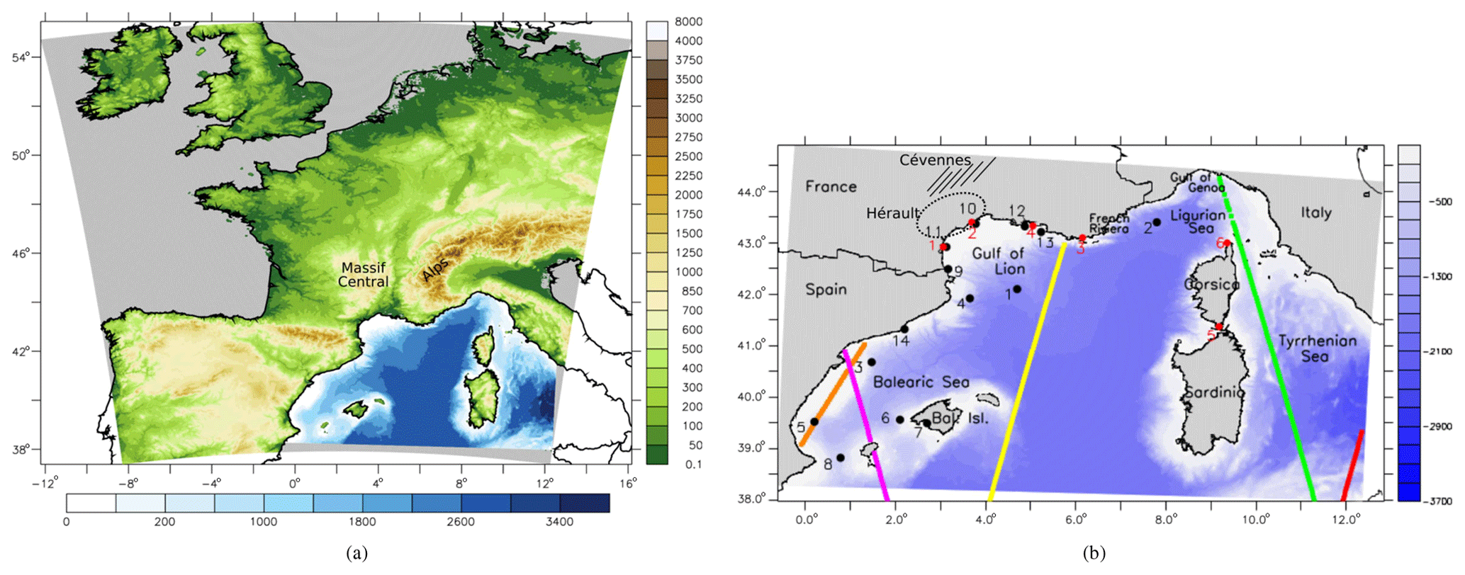
Figure 1Simulation domain: (a) AROME-France (topography, m) and (b) the WW3 domain illustrated with bathymetry (blue scale, m). Black circles indicate the locations of the moored buoys, and red circles denote the locations of the surface stations (see Table 1). The satellite track around 05:00 UTC on 12 October is shown in green, the satellite track around 18:00 UTC on 13 October is shown in yellow, the satellite track around 05:00 UTC on 14 October is shown in magenta and the satellite track around 18:00 UTC on 14 October is shown in red and orange – the orange track is for JASON-2 and the other tracks are for SARAL.
2.2 The wave model
The wave model is WaveWatch III (hereafter WW3, version 5.16, The WAVEWATCH III Development Group, 2016; Tolman, 1992). The model domain covers the north-western Mediterranean Sea at a 1∕72∘ horizontal resolution (Fig. 1b). The bathymetry is sourced from the NEMO-NWMED72 ocean model configuration described in Sauvage et al. (2018b), which was originally built from the interpolation of a 1∕120∘ horizontal resolution topography with a dedicated treatment for island, coastline and river mouth delineation. The time step is 60 s.
The set of parameterizations from Ardhuin et al. (2010) is used, as for most of the wave forecasting centres (Ardhuin et al., 2019). Thus, the swell dissipation is computed with the Ardhuin et al. (2009) scheme, and the wind input parametrization is adapted from Janssen (1991). Nonlinear wave–wave interactions are computed using the discrete interaction approximation (DIA, Hasselmann et al., 1985). The parametrization of the reflection by shorelines is described in Ardhuin and Roland (2012). Moreover, the computation of the depth-induced breaking is based on the algorithm from Battjes and Janssen (1978), and the bottom friction formulation follows Ardhuin et al. (2003).
2.3 Atmosphere–wave coupling
2.3.1 Bulk iterative equations
The sea surface turbulent fluxes are calculated through the bulk formulae described as follows:
where ρ is the air density, cpa is the air heat capacity and Lv is the vaporization heat constant. ΔU, Δq and Δθ represent the air–sea gradients of velocity, specific humidity and potential temperature near the surface respectively. CD, CE and CH represent the transfer coefficients. Each transfer coefficient can be defined as follows:
where x is d for wind speed, θ for potential temperature and q for water vapour humidity. Therefore,
and
where the subscript n refers to neutral (ζ=0) stability, z refers to the reference height and ψx is an empirical function describing the stability dependence of the mean profile; κ is the von Karman constant.
The sea surface roughness length z0 is defined by two terms: the Charnock's relation (Charnock, 1955) and a viscous contribution (Beljaars, 1994).
where ν is the kinematic viscosity of dry air, u* is the friction velocity and αch is the Charnock coefficient.
2.3.2 Wave impact on the Charnock coefficient
One common method of coupling developing waves and stress is to make the Charnock coefficient αch explicitly dependent on the sea state by computing it either in the wave model from the wave spectra (e.g. Janssen et al., 2001) or in the atmospheric model as a function of the wave age (Mahrt et al., 2001; Oost et al., 2002; Moon et al., 2004). Studies based on observations (e.g. Oost et al., 2002) express it as a power function:
where coefficients A and B are either constant or depend on the surface wind speed, and the wave age χ is defined as (where cp is the peak phase speed, and Ua is the near-surface wind). Sea state can mainly be defined using the wave age. “Wind sea” corresponds to waves, generated by local wind, that are still growing (wave age <0.8) or in equilibrium with the wind (wave age between 0.8 and 1.2) and are aligned with the local wind. These waves (and only these waves) benefit from momentum transfer from the atmosphere to grow; thus, they are coupled to the wind. Conversely, swell (which does not depend on the momentum from the atmosphere) corresponds to waves generated by a remote or past wind field and is characterized by a wave age above 1.2 or waves that are not aligned with the local wind.
Assuming that the water depth is infinite (in practice, as soon as the depth is much larger than the dominant waves), the phase speed of the waves can be expressed as
where Tp is the peak period of the waves and g is the acceleration of gravity.
Keeping the coefficients A and B constant with wind speed results in drag coefficient and wind stress values that are too strong under strong wind conditions (a wind speed above 20 m s−1), as shown by Pineau-Guillou et al. (2018). In order to tackle this, and to reproduce the saturation or the decrease in the drag coefficient observed under strong to cyclonic wind conditions (e.g. Powell et al., 2003), we take advantage of a new parameterization called WASP (Wave-Age-dependant Stress Parametrization). This approach considers that the wind speed range where the wind stress transferred to the sea surface mainly sustains the wave development (through interaction with non-breaking waves) is between 5 and 20 m s−1. Above 20 m s−1, the contribution of breaking waves to the wave stress is dominant and the wave age is not an appropriate parameter to represent the sea state effect on the surface roughness. Below 5 m s−1, under very weak wind conditions, the surface roughness is mainly controlled by the viscous term (second term on the right-hand side of Eq. 7). In order to reproduce these different mechanisms as well as the decrease in the drag coefficient under very strong wind conditions, the Charnock parameter of the WASP parameterization is piecewise continuously defined following Eq. (8), with the coefficients A and B being polynomial functions of the surface wind speed (see Appendix A). Under weak to strong wind regimes where wind stress observations are numerous and consistent with each other (i.e. until 23 m s−1), WASP has been fitted to datasets used to build the COARE 3.5 parameterization (Edson et al., 2013). The temperature and humidity roughness lengths z0T and z0q (see Eq. 6), which define the corresponding neutral transfer coefficients, have been adjusted for the resulting sensible and latent heat fluxes to match the COARE 3.0 (Fairall et al., 2003) parametrization for surface wind speeds up to 45 m s−1. The stability functions ψx (Eq. 5) are a blend of the Kansas-type functions (Businger et al., 1971) and a profile matching the asymptotic convective limit (Fairall et al., 1996).
Thus, WASP enables us to represent the Charnock parameter's behaviour and its dependency on waves in a more physical way. Moreover, it reproduces the observed decrease in the drag coefficient due to very strong wind, which would not be possible using a wave-age-only Charnock parameter as in Drennan et al. (2005). Therefore, WASP is more relevant for atmosphere–wave coupling and for high to very high wind speeds.
2.3.3 Coupling
The coupling is performed using the SURFEX-OASIS coupling interface (Voldoire et al., 2017) that manages the exchanges between the AROME and WW3 models. AROME-SURFEX provides the two components of the near-surface wind speed to WW3, whereas WW3 provides Tp (the peak period of the wind sea) to AROME-SURFEX. The OASIS coupler (Craig et al., 2017) allows one to choose the coupling frequencies and the interpolation methods for the exchanged fields.
Furthermore, as the AROME domain is larger than the WW3 domain (in particular, also covering a part of the Atlantic Ocean), there is no air–wave coupling for the marine zones not covered by WW3 (i.e. for the grey zones in Fig. 1a); thus, in these regions, χ is directly estimated in WASP as a function of wind with and, in turn, . This can be found using the relation , where cp is approximately 5 for a typical nondimensional fetch and the gravity constant, g, is approximately 10.
2.4 Set of simulations
In this study, three kinds of simulations were examined: wave-only, atmosphere-only and wave–atmosphere coupled simulations. As the objective of this study is to better assess the role of the waves on the dynamics (i.e. the impact on the momentum flux and surface wind) as well as the impact on the sea surface turbulent heat fluxes, a common and fixed sea surface temperature (SST) is used in all the experiments and no ocean coupling is introduced so that the wave effects on these fluxes are not masked.
First a wave-only simulation (named WY) was run. For this simulation, WW3 ran from 5 to 15 October 2016 with the initial conditions (Hs, Tp) set to zero and a near-surface wind forcing sourced from AROME forecasts at an hourly frequency (+1 to +24 h each day, see Sauvage et al., 2018a). The period from 5 to 12 October served here as a spin-up period and will not be considered in the following. Boundary conditions for the wave model consisted of eight spectral points distributed along the domain and provided by a WW3 global 1∕2∘ resolution simulation run at Ifremer (Rascle and Ardhuin, 2013). These points (each defined following 24 directions and 31 frequencies) were chosen as close to our domain border as possible from the output points available from the WW3 global simulation. They were then linearly interpolated onto our grid () in the WW3 preprocessing routine.
Atmosphere-only simulations were carried out with AROME. Each AROME simulation was composed of forecast runs that started every day (12, 13 and 14 October 2016) at 00:00 UTC from AROME operational analyses and that lasted 42 h. Hourly boundary conditions were sourced from the ARPEGE (Action de Recherche Petite Echelle Grande Echelle, Courtier et al., 1991) operational forecasts except for the SST, which came from the global daily analysis of the Mercator Océan International (1∕12∘ resolution PSY4 system, Lellouche et al., 2013). The first atmosphere-only (AY) simulation was carried out without any wave information, meaning that χ was set as a function of the near-surface wind with . The second atmosphere-only run (AWF) was forced by the hourly wind sea Tp from the WY simulation.
Finally, a two-way coupled AROME-WW3 simulation (AWC) was undertaken following the description given in Sect. 2.3.3. The SST field and the atmospheric initial and boundary conditions of AWC were the same as in the atmosphere-only simulations. Moreover, the wave boundary conditions in AWC were the same as for WY. Wave initial conditions were sourced from restart files: first from WY for the forecast starting at 00:00 UTC on 12 October, and then from the previous AWC forecast run for the following days (after 24 h). The coupling frequency was set to 1 h in both directions. Each exchanged field was interpolated using a bilinear method.
3.1 Available observations
In order to validate the simulations, we collected several observations of the surface and near-surface in the north-western Mediterranean area (see Fig. 1b, which displays the observations over the WW3 domain).
Table 1Names and locations of the moored buoys and surface stations (in italics) used for validation. The numbers given in front of the names refer to Fig. 1b.
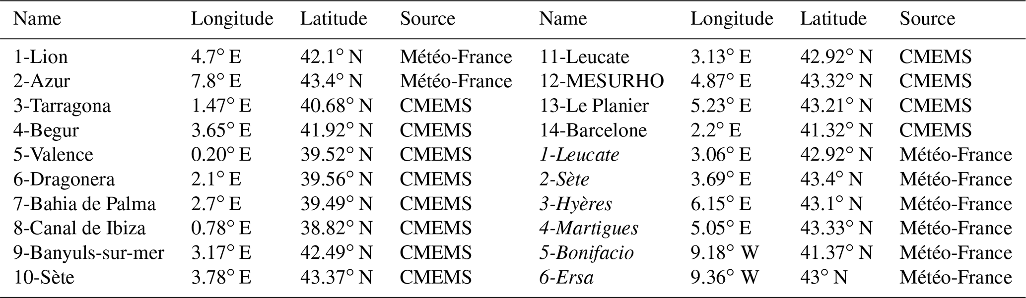
Data from 14 moored buoys (listed in Table 1 and plotted in Fig. 1b), available either from the Copernicus Marine Environment Monitoring Service (CMEMS, http://marine.copernicus.eu/, last access: 3 Feruary 2020) database or from the HyMeX programme database (http://mistrals.sedoo.fr/HyMeX/, last access: 3 Feruary 2020), were first used for validation. These platforms measure a wide variety of near-surface variables that may include sea temperature, salinity and wave parameters, such as the significant wave height (Hs) and peak period (Tp), as well as some atmospheric parameters, such as the 2 m air temperature, relative humidity, the 10 m wind speed, wind direction and gusts. In addition to these buoys, six coastal surface weather stations from the Météo-France network were used (mainly around the Gulf of Lion and in Corsica) in order to complete the coverage over the area of interest with respect to atmospheric in situ data. Altimetric data from two satellites crossing the area during the event were used for the significant wave height validation. The first satellite was Jason-2 (OSTM/Jason-2 Products Handbook, 2008) from the joint CNES/NASA oceanography mission Jason. The altimetric measurements used were the Geophysical Data Record (GDR) from the MLE4 (maximum likelihood estimator) altimeters' retracking algorithm that were corrected following a buoy comparison method: . The second dataset was obtained from GDR data from the SARAL/AltiKa satellite (SARAL/AltiKa Products handbook, 2013) that also uses the MLE4 altimeters' retracking algorithm but simply removes erroneous Hs using a threshold relationship. Both satellites combined gathered 292 measures of Hs during the period between 12 and 14 October 2016.
To validate the rainfall accumulation, the ANTILOPE product from Météo-France was used (Laurantin, 2008). This product merges rain gauges and radar data. This analysis was complemented by the use of the Météo-France radar composite images over western Europe.
3.2 Validation of AWF and WY
For the validation of our wave and atmospheric reference simulations, WY and AWF respectively, the time series from 12 to 14 October were built using the first 24 h of simulation starting each day (Fig. 2). Observations and simulations were compared using the nearest grid point in space and time from the model (WW3 or AROME) to the observation grid point. The bias, the root-mean-square error (RMSE) and the correlation were computed and are summarized in Table 2.
Table 2Skill scores computed against surface stations and satellite data for the wave-only simulation (WY) and the coupled simulation (AWC) for wave parameters (Hs, Tp) and for the atmosphere-only simulations (AY and AWF) and coupled simulations (AWC) for atmospheric parameters. WSP represents 10 m wind speed (m s−1), WDIR represents 10 m wind direction (∘), T2m represents 2 m air temperature (∘C) and RH2M represents 2 m relative humidity (%).
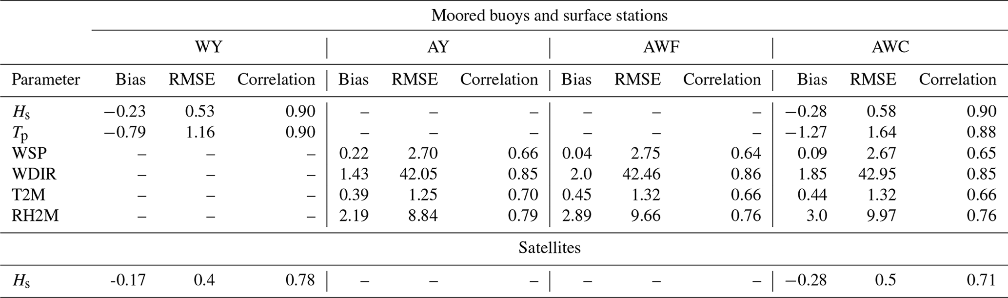
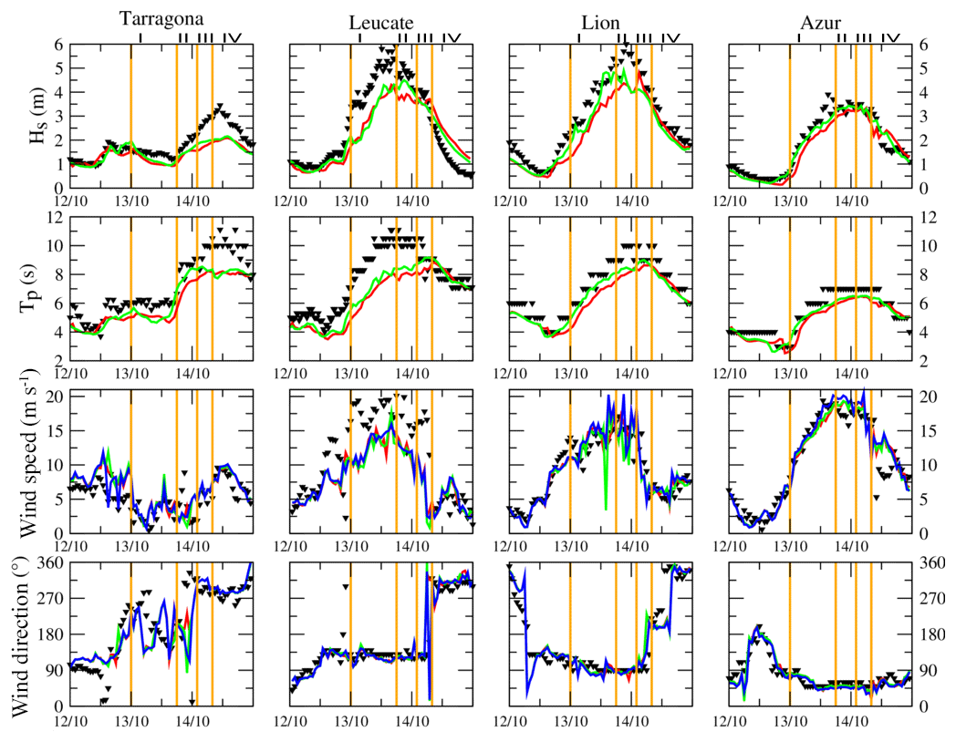
Figure 2Evolution of Hs (m), Tp (s), wind speed (m s−1) and wind direction (∘) simulated with AWF–WY (green), AWC (red) and AY (blue) against buoy observations (black triangles).
During the entire event, the sea state appeared to be well represented by WY with a correlation of 0.90 for Hs and Tp. Looking at Fig. 2, Hs and Tp seemed to be underestimated during the event. This was confirmed by a negatives bias of −23 cm for Hs and −0.79 s for Tp as well as by the comparison of the simulated Hs against satellite data that showed an average bias of about −0.17 cm (Table 2). However, a good correlation of 0.78 was obtained with satellite data.
In AWF, the wind speed and direction were quite well represented with correlations of 0.64 and 0.86 respectively (Table 2), although they were very slightly overestimated during the event with an averaged bias of 0.04 m s−1 and 2∘ respectively. Looking at the wind speed correlation over different regions, i.e. the Gulf of Lion and the Balearic Sea, some differences can be highlighted. In the Gulf of Lion and along the French Riviera, a correlation coefficient of 0.82 was found. Looking at the buoys located in the Balearic Sea, i.e. where the wind was weaker, the simulation represents the wind speed value well but a low correlation (0.45) is found.
By looking at the French western coastal buoys in more detail, such as Leucate (Fig. 2) which is located on the most western part of the Gulf of Lion, a large underestimation of the wind speed was found. The observed wind speed reached values of between 18 and 20 m s−1 several times, whereas the simulation only reached 15 m s−1. In addition, at Sète, the wind intensity was in good agreement but decreased faster than observed (not shown). There is also a delay at the end of the event between the simulation and observations, which is notable at the Lion buoy (Fig. 2) when a transition to a northerly wind occurred.
The validation against in situ data for the 2 m air temperature (T2M) and relative humidity (RH) (Table 2) showed that AWF represented these two atmospheric parameters quite well with correlation coefficients of 0.68 and 0.78 respectively, despite small overestimations (averaged biases of 0.26 ∘C and 2.23 % respectively). These scores, along with the validation against low-level wind and wave parameters, gave us confidence in the use of AWF with respect to investigating the evolution of the turbulent fluxes at the air–sea interface during the abovementioned HPE.
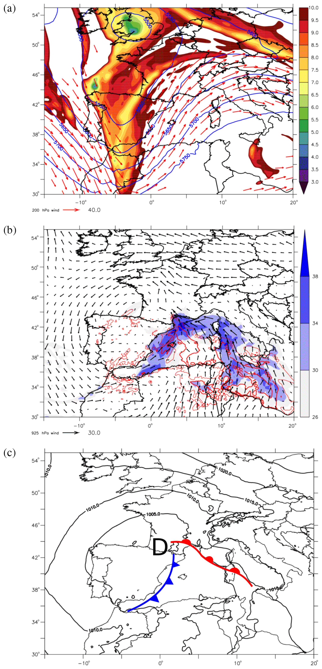
Figure 3Synoptic situation at 12:00 UTC on 13 October 2016 from the ARPEGE analysis (a) at high level: the coloured shading is the height of the 2 PVU (potential vorticity units) isosurface (km), the blue contours are the geopotential height (m) at 500 hPa and the red arrows denote the wind above 20 m s−1 at 200 hPa. Synoptic situation at 12:00 UTC on 13 October 2016 from the ARPEGE analysis (b) at low level: the coloured shading is the integrating water vapour (kg m−2), the red contours are the convective available potential energy (J kg−1) and the black arrows denote the wind at 925 hPa. Panel (c) shows the mean sea level pressure (black contours) and position of the cold (blue) and warm (red) fronts.
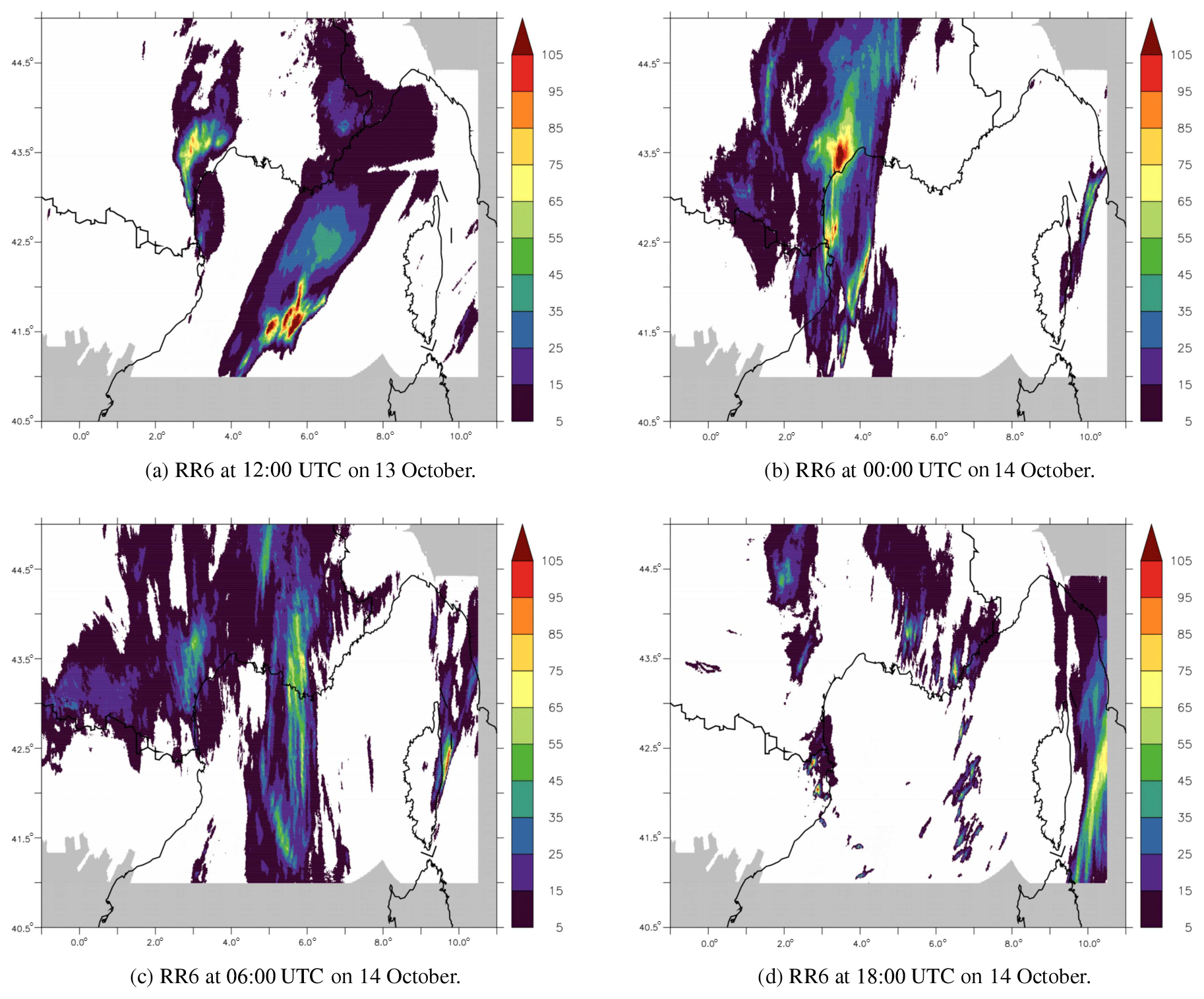
Figure 4The 6 h rainfall amounts (mm) from ANTILOPE observations.
The HPE studied occurred between the 13 and 14 October 2016 over the north-western Mediterranean Sea. This event could be defined as a typical “Cyclonic Southerly” (CS), following the four classifications of synoptic types from Nuissier et al. (2011). Indeed, the synoptic meteorological situation (Fig. 3) was characterized by a trough at altitude extending from the British Islands to Spain and associated with a lowering of the tropopause (Fig. 3a) that induced a south-westerly flow over south-eastern France. A cyclonic circulation took place at low levels (Fig. 3b) with a high moisture content over the Gulf of Lion and a strong south-easterly flow that originated from south-eastern Tunisia. During the night and the following day, the trough moved eastwards from the Bay of Biscay to the Gulf of Lion along with cold and warm fronts (Fig. 3c), and the low-level flow also shifted eastwards.
The HPE was characterized by four periods that can be distinguished using observations over land and the reference simulation (AWF) for the marine low-level conditions: (i) initiation stage, (ii) mature systems, (iii) north-eastward propagation and (iv) tramontane wind onset. In the following, a detailed description of the chronology of the event and the mechanisms involved is carried out. For this purpose, the 42 h forecast starting at 00:00 UTC on 13 October 2016 from AWF was used along with observations.
4.1 Chronology of the convective systems
Phase I, from 03:00 to 18:00 UTC on 13 October 2016 (+3 to +18 h in the simulation), was marked by the triggering of deep convection and the stationarity of the two main systems. The first deep convective system was triggered in the Cévennes foothills, south of the Massif Central, (Figs. 1, 4a, 5a), where the unstable rapid south-easterly marine flow encountered orography (Fig. 5c). The second deep convection system was a MCS associated with large precipitation over the sea (Figs. 4a, 5a). It formed at the convergence between the warm south-easterly flow, associated with high CAPE values, and the colder and drier easterly flow from the Alps and Ligurian Sea (Fig. 5c, d). These two convective systems were well represented in the reference simulation (Figs. 4a, 5a) in terms of location and rainfall amounts compared to observations. The simulated radar reflectivities also corresponded quite well to observations (not shown) except in north-eastern Spain where overly active convective systems were simulated.
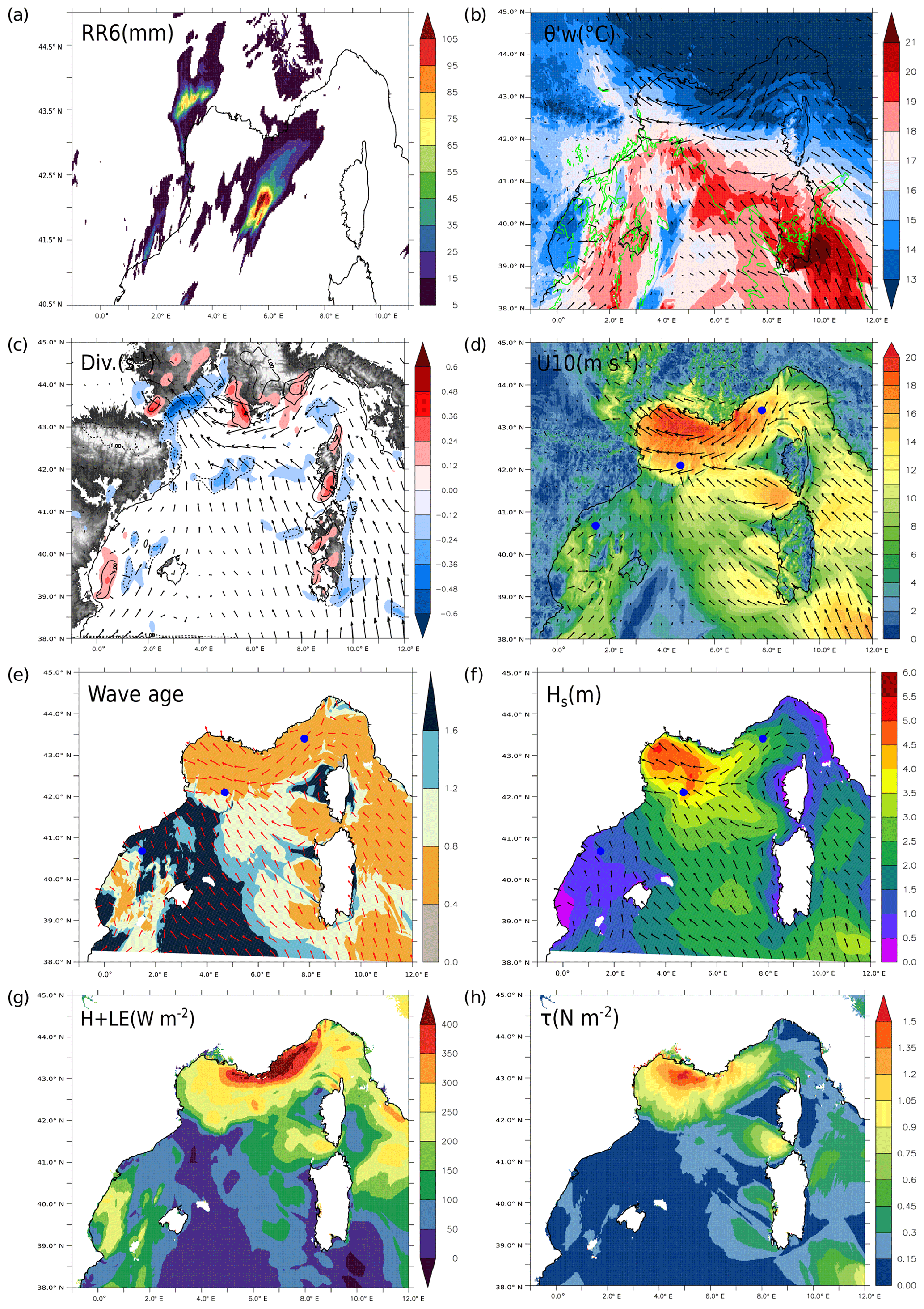
Figure 5(a) The 6 h rainfall amount (mm). (b) The pseudo-adiabatic potential temperature θw' (coloured shading, ∘C) and wind (m s−1, arrows) at 925 hPa with the CAPE over 750 J kg−1 shown using green contours. (c) The wind divergence (coloured shading, 10−3 s−1, values between -0.12 and 0.12 are masked) at 950 hPa, where the black contours are the vertical velocity (Pa s−1) at 950 hPa and the black arrows are the horizontal winds (m s−1). (d) The 10 m wind intensity and direction (m s−1). (e) The wave age and wave direction. (f) The wave significant height (m) and wave direction. (g) The total turbulent heat fluxes (H, LE) (W m−2). (h) The wind stress (N m−2) simulated by AWF at 12:00 UTC on 13 October. Blue dots in (d), (e) and (f) represent the Tarragona, Lion and Azur buoys (from west to east).
During Phase II, from 19:00 UTC on 13 October to 03:00 UTC on 14 October (+19 to +27 h in the simulation), the precipitating system over the Hérault region remained stationary. Its intensity increased in the observations (Fig. 4b), whereas precipitation totals for the second system over the sea decreased. In AWF, the simulated precipitating system over the sea started to shift towards the east, while precipitation over the Hérault region decreased (Fig. 6a). The simulated cold front progressed eastwards earlier than in the observations; thus, the southern flow also started to shift (Fig. 6d) as did the convergence line over the sea (Fig. 6c).
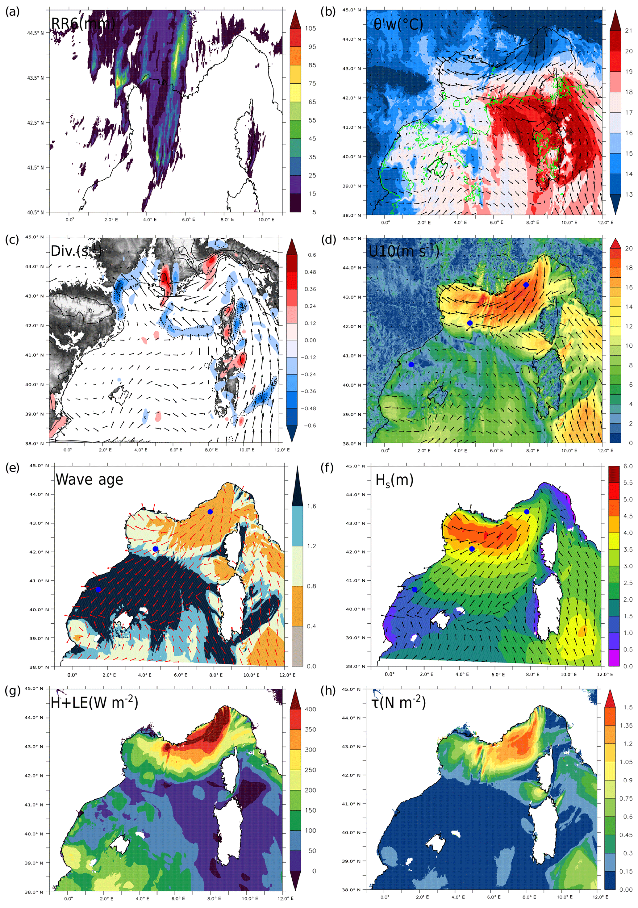
Figure 6Same as for Fig. 5 but at 00:00 UTC on 14 October.
Phase III, from 04:00 to 10:00 UTC on 14 October (+28 to +34 h in the simulation), was marked by the north-eastward propagation of the system. As the western front was moving eastwards, the system over the Hérault region shifted toward the French Riviera (Fig. 7c), leading to a local decrease in the precipitation total (<60 mm over the Hérault region, Fig. 4c). In the simulation, the system over the sea also moved eastwards, extending from west of Corsica to the French Riviera, and there was a decrease in the rainfall amounts (Fig. 7a). It appeared that the simulated eastward propagation was earlier than observed. The southerly flow was also consistently shifted and was located between Corsica–Sardinia and continental Italy (Fig. 7d) with a main convergence area over the Ligurian Sea. At the same time, the intensity of the inland system (over the Hérault region) was overestimated compared with observations (Figs. 4c, 7a).

Figure 7Same as for Fig. 5 but at 06:00 UTC on 14 October.
The last phase (Phase IV), from 11:00 UTC on 14 October (+35 h to the end of simulation, not shown), was characterized by the end of the precipitation over France (Fig. 4d) and the beginning of a new wind regime in the Gulf of Lion, with a dry and cold north-westerly flow corresponding to the regional tramontane wind regime. Thus, the warm southern flow was limited to the south-east of the simulation domain and fed the precipitating system located from the northern Sardinian region to continental Italy (Fig. 4d). For this period, the simulation was in good agreement with observations in term of rainfall locations and amounts.
4.2 Evolution of the sea state
Three different areas can be distinguished in our domain, mainly represented by the three moored buoys (Fig. 1, Table 1).
-
The Tarragona buoy, where the wind was weak, was situated in a long fetch area. There was swell throughout the event, first aligned with the south-easterly wind in Phase I and then crossed, as wind and waves were opposite.
-
The Lion buoy was located where the easterly wind was stronger during Phase I, generating a young wind sea with strong Hs. It evolved to a well-developed wind sea during Phase II and then to a swell as the fetch became longer in this area.
-
The Azur buoy was located in the strong easterly wind throughout the event. Characterized by a short fetch, a wind sea was continuously produced in this area.
During Phase I, a strong easterly wind (between 15 and 20 m s−1; Figs. 2, 5b) affected the Ligurian Sea, from the French Riviera to the Gulf of Lion. This created a wind sea, with young waves (see the Azur buoy in Figs. 5e and 8) aligned with the wind and associated with moderate Hs (<3 m, Fig. 5f). In fact, the waves in this area were directly generated by the local wind throughout the event (Fig. 8) with low wave age values (<1) and a similar direction between wind and waves. In the Gulf of Lion, a rough to very rough sea was observed (Hs∼4–5 m) that was associated with a Tp of about 8 s (Fig. 2). Still, a weak wave age (Figs. 5e, 8) was found here due to strong winds. Thus, the waves in this area were mainly generated by the wind above.

Figure 8Evolution of the wave age (blue) and direction (∘) of local wind (red) and waves (black) simulated with AWF (WY) during the 13 October run at three different moored buoys. Orange lines limit the four different phases (I, II, III and IV).
In the Balearic Sea high wave ages were simulated (>1.2, Fig. 8) under a weak south-westerly flow (Fig. 2); this induced a weaker Hs, which corresponded to a moderate sea. The sea state in this area was consistent with a swell coming from the south.
During Phase II, Tp reached a maximum (∼10 s observed) in the Gulf of Lion; Hs values were also highest in this region (about 6 m), corresponding to a very rough sea which is rather exceptional in the Mediterranean Sea. This well-developed wind sea (wave age between 0.8 and 1.2) was due to the continuous easterly wind that had been blowing since Phase I (Figs. 2, 6b). The intensity of the easterly flow decreased in the Gulf of Lion but increased in the Ligurian Sea (±2–3 m s−1; Figs. 2, 6b). In the Balearic Sea, the wave ages were still high but the wave direction changed progressively from easterly to north-easterly. This corresponded to the swell coming from the Ligurian Sea, as a weak south to north-westerly wind (<10 m s−1) was blowing locally (Figs. 2, 6b, e, 8).
During Phase III, Hs started to decrease over the domain (Figs. 2, 7f) and the observed Tp reached a maximum in the Balearic Sea and in the western part of the Gulf of Lion, which was associated with swell (Figs. 2, 7e, 8). As the front moved eastwards, a significant decrease in the easterly wind was observed (up to −7 m s−1; Figs. 2, 7b), whereas the wind speed was strongest in the Gulf of Genoa. Indeed, the wind in the Gulf of Lion started to change direction with a transition to a northerly wind (see Leucate, Sète and Lion in Fig. 2). As in the Balearic Sea (Figs. 7e, 8), the wind changed direction from north-westerly to westerly.
Finally, during Phase IV, Hs kept decreasing over the domain (<3 m, Fig. 2). Tp significantly decreased in the Gulf of Lion, whereas the highest values were still located in the Balearic Sea (Fig. 2). At both locations, the swell generated along the French Riviera was present (Fig. 8), while the easterly wind significantly decreased (now <14 m s−1, Fig. 2). The onset of a north-westerly wind (Tramontane) in the Gulf of Lion was observed (Fig. 2), while a westerly wind was blowing over the Balearic Sea.
4.3 Air–sea interface
The latent heat flux (LE) was quite low over the domain, as displayed by Fig. 5g. During Phase I, the cold and dry air from the Alps became rapidly warmer and more humid as it flowed westwards over the sea. Evaporation started in this area and also marked the location of the largest LE values (over 300 W m−2, Fig. 5g). In addition, this region was characterized by the strongest humidity transport, due to the easterly flow, towards the Gulf of Lion as the air humidity increased (over 94 %). Under a strong easterly wind, along the French Riviera, the difference between SST and T2M was up to 4 ∘C (5 ∘C locally) and, thus, with high sensible heat flux (H) values (over 150 W m−2, Fig. 5g). The warm (>23 ∘C) and humid (over 85 %) southern flow did not produce large heat fluxes (Fig. 5g). It can be noticed that there was warm and dry air masses in the Balearic Sea, but the weak south-westerly wind blowing in this area limited evaporation and heat fluxes. The momentum flux was the largest under the strong easterly wind in the Gulf of Lion – reaching up to 1.5 N m−2, whereas it reached up to 1.2 N m−2 locally under the south-easterly flow (Fig. 5h). It remained lower than 0.3 N m−2 throughout the rest of the domain.
As the system moved eastwards during Phase II, the rapid low-level flow moved from the Gulf of Lion to the Ligurian Sea. The evaporation kept increasing in this area, and the dry air in the Gulf of Genoa became almost saturated in the Gulf of Lion. The largest values of the momentum flux were located along the French Riviera at this time (Fig. 6h). LE decreased by more than 50 W m−2 in the Gulf of Lion and increased along the French Riviera and the Gulf of Genoa, reaching more than 360 W m−2 (Fig. 6g). As the cold front was shifting, the low-level air mass in the Balearic became drier and pushed the humid southerly flow to the east. The highest values of H were also shifted in the Gulf of Genoa and reached 200 W m−2 (Fig. 6g), whereas H significantly decreased in the Gulf of Lion.
During Phase III, drier air (RH <70 %) was located from the Balearic Sea to the coast of Sardinia. In the Gulf of Lion, low-level air continued to get drier, whereas moist air was now mainly located along the French Riviera and in the Gulf of Genoa (where precipitation occurred). Under precipitation, H increased to 250 W m−2 (Fig. 7g). LE significantly decreased by 100 W m−2 along the French Riviera but was still highest in the Gulf of Genoa (Fig. 7g). A large decrease (of 1 N m−2) was also noticed in the momentum flux along the French Riviera and maximum values were found in the Gulf of Genoa (Fig. 7h).
During the last phase (Phase IV), with the large decrease in the wind intensity and the precipitation now located over Italy, RH decreased along the French Riviera and in the Gulf of Genoa in association with a large decrease (of 150 W m2) in the heat fluxes. The momentum flux was lower than 0.3 N m−2 in the Gulf of Genoa at this time.
A rapid analysis of the relationship between the heat fluxes (H and LE) and atmospheric parameters (Ua, temperature gradient, humidity gradient) was carried out using scatterplots (not shown). It highlighted that the sensible heat flux was more correlated with the temperature gradient at the air–sea interface (0.56), which was related to the cold air present in the easterly flow or below precipitation. Conversely, the latent heat flux was more correlated with the wind (0.49) than with the gradient of humidity (0.31). In summary, the maximum turbulent fluxes were associated with the easterly low-level jet due to strong winds and large air–sea temperature (moisture) gradients for heat fluxes. In the southerly flow, heat fluxes appeared more limited despite moderate wind. This highlighted the role of the Ligurian easterly flow in extracting heat and moisture from the sea and in providing them to the MCSs.
Finally, looking at the different phases of the event, some areas emerged as potential regions where the waves should have an impact on the low-level flow. Indeed, during phases I and II, an effect on the momentum flux was expected in areas of strong easterly wind and of wind sea, especially over the French Riviera and the Gulf of Lion in Phase I. These regions were also the places with the highest heat fluxes during the event and, thus, were more likely to be affected by the sea state. Therefore, the sensitivity to the impact of the representation of sea state will be particularly investigated in these areas in the following.
In this section, the goal is to better understand the impact of the waves on the sea surface turbulent fluxes and to evaluate the impact on the HPE forecast. We focused on phases I and II, at 14:00 UTC on 13 October and 00:00 UTC on 14 October 2016, respectively (corresponding to +14 and +24 h of forecast respectively, starting at 00:00 UTC 13 October). In order to examine the mechanisms at the air–sea interface and the effects of waves on the HPE in a continuous way during these two phases, the sensitivity analysis was carried out considering the 42 h of forecast starting at 00:00 UTC on 13 October.
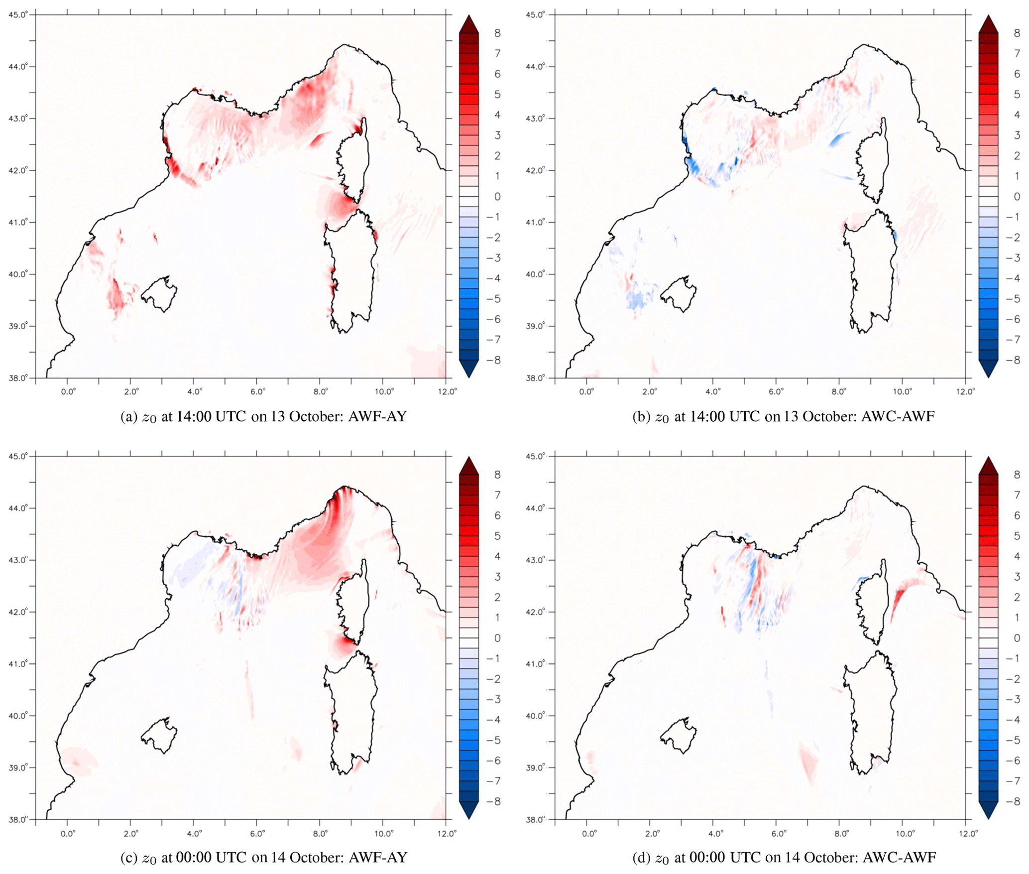
Figure 9z0 (10−3 m) differences at 14:00 UTC on 13 October (a, b) and at 00:00 UTC on 14 October (c, d) between AWF–AY (a, c) and AWC–AWF (b, d).
5.1 Low-level flow
5.1.1 Impact of the waves: AWF versus AY
In the following, AWF, which takes the sea state into account, is compared to the atmosphere-only simulation, AY (see Sect. 2.4). Figure 9a and c present the difference in the sea surface roughness length (z0) between AWF and AY. During Phase I, an increase in z0 (from to m) in AWF was found (compared with AY) over the wind sea under a strong easterly wind in the Gulf of Lion and along the French Riviera. Throughout the rest of the domain, much smaller z0 differences were noticed (less than m). These changes induced an increase in the drag coefficient Cd of up to and led to an increase in the momentum flux of more than 0.1 N m2. Finally, this increase in the momentum flux resulted in a decrease of more than 1 m s−1 in the 10m wind speed intensity of the strong easterly flow over a large area between the Gulf of Lion and the French Riviera (Fig. 10a). During Phase II, along the French Riviera and the Gulf of Genoa, characterized by the strong easterly wind and a young wind sea (Fig. 6b, e), z0 increased by more than m and up to m in AWF compared with AY (Fig. 9c). Knowing that z0 barely exceeds m in AY, these differences correspond to an increase of more than 100 % of the values in AY. Under the convective system some difference dipoles were found. In the Gulf of Lion, a slight increase in z0 was seen. While differences in z0 in Liguria were observed from the beginning of the simulation, differences under the MCS and in the Gulf of Lion appeared to result from differences in the movement of the convective system over the sea, which were induced by the decrease in the wind intensity during Phase I. Due to the same mechanisms as in Phase I, the increase in z0 upstream of the MCS (i.e. along the French Riviera) directly impacted the Cd, which increases in AWF by to more than locally. This led to an increase in the wind stress of between 0.1 and 0.3 N m2 in this area and resulted in a slowdown of between 1 and 2 m s−1 the 10 m in the wind speed along the French Riviera (Fig. 10c). Larger differences were found under the convective system but appeared inhomogeneous in space and time. Thus, the results confirmed the primary effect of the representation of sea state as notably highlighted by Thévenot et al. (2016) and Bouin et al. (2017): when the sea state is taken into account, an increased surface roughness and wind stress are observed that slow down the upstream low-level flow.
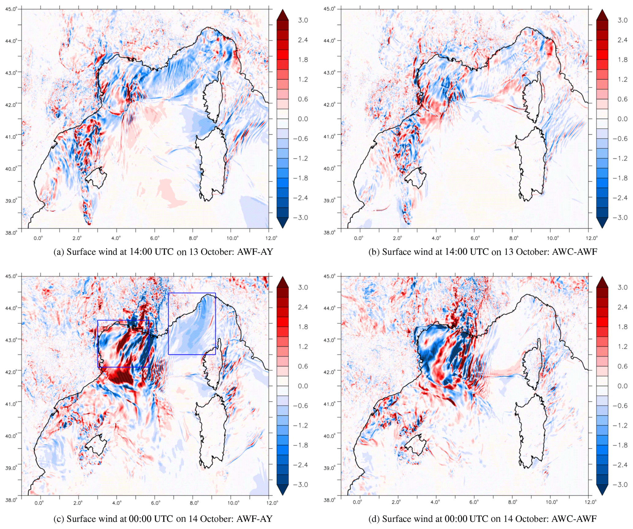
Figure 10Surface wind (m s−1) differences at 14:00 UTC on 13 October (a, b) and at 00:00 UTC on 14 October (c, d) between AWF–AY (a, c) and AWC–AWF (b, d).
In the two subareas delineated in Fig. 10c, it was found that, on average, a slowdown of the 10 m wind speed was obtained in both areas during the four phases. Specifically, an averaged slowdown of 0.9 m s−1 was noticed in the Gulf of Lion during the Phase I. This represented a decrease of about 6 % of the average wind intensity in AWF. The same result was found during Phase II along the French Riviera with an average decrease of 0.9 m s−1 (−7 %). Scores did not appear to be change significantly between AWF and AY (Table 2). However, a lower bias in the wind intensity was found (0.04 m s−1 in AWF compared with 0.22 m s−1 in AY) and was actually mostly due to a large improvement at the Azur buoy, where the bias was reduced from 0.42 m s−1 in AY to 0.08 m s−1 in AWF.
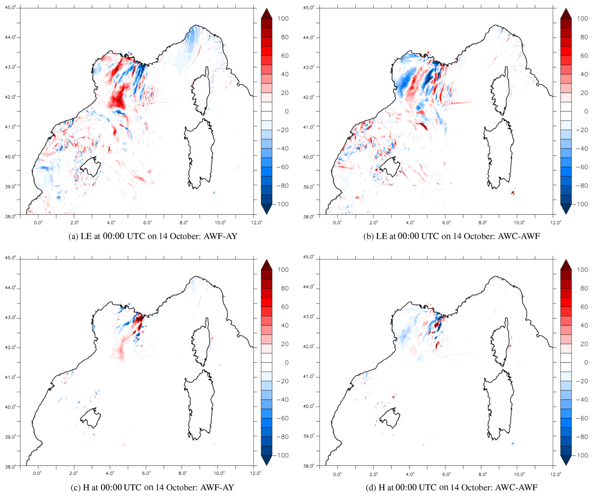
Figure 11(a, b) LE (W m−2) and (c, d) H (W m−2) differences at 00:00 UTC on 14 October between AWF–AY (a, c) and AWC–AWF (b, d).
Figure 11a and c present the heat flux (the latent and sensible fluxes respectively) differences between AWF and AY. Along the French Riviera, where the latent heat flux was the strongest, a decrease was obtained in AWF during phases I and II. However, this corresponded to a small decrease (5 W m−2 on average) that was equivalent to 2 % of the total averaged latent flux. Relatively larger differences, both positive and negative, were found under the convective system. However, on average, these differences were small, representing ±2 % (3 W m−2). They were very likely related to differences in terms of the intensity of the convection within the MCS and its location and were not a direct effect of the waves. Differences in the sensible heat flux (Fig. 11c) were mainly located under the precipitation with very weak differences along the French Riviera.
5.1.2 Impact of the coupled system: AWF versus AWC
Figure 9b and d present the differences in z0 between AWF and the atmosphere–wave coupled system AWC. During Phase I, z0 in AWC increased by up to m over the French Riviera and the eastern part of the Gulf of Lion (Fig. 9b). As a result, a slight decrease in the 10 m wind speed intensity was found in this region, about 0.6 m s−1 (Fig. 10b). During Phase II, smaller differences were obtained along the French Riviera. This corresponded to a small increase in z0 in AWC of about m under a strong easterly wind (Fig. 9d). The 10 m wind speed was decreased in AWC by no more than 0.3 m s−1 (Fig. 10d). The smaller impact on the low-level dynamics in AWC can be explained by the feedback of the wind on the waves. Indeed, on average, it was found that Hs was decreased by 12 % and Tp by 7 % in AWC during the event. As we already had an underestimation of the wave parameters in WY, this decrease in AWC induced larger biases (Table 2). Larger differences in the wind intensity were also found under the convective system and downstream of it in the Gulf of Lion (Fig. 10d). However, these were not really consistent throughout the simulation and were mainly due to the movement of the system and the slowdown of the wind during Phase I.
Figure 11b and d illustrate the differences in the heat fluxes. Very small variations were noticed for either LE or H (less than 10 W m−2) along the French Riviera. As before, the larger differences in the Gulf of Lion were more likely to have been induced by the movement and the convective cell evolution of the MCS.
Thus, on average, coupling only showed minor effects on the dynamics and on the heat and moisture exchanges below the upstream low-level flow. One main explanation for this small effect might be that the waves used in AWF and AWC were really close to each other in term of spatial and temporal resolution, both simulated using WW3. Locally, effects on the dynamics can be significant; this is especially true in strong wind and wind sea areas, where we found a decrease in the wind speed and in Hs and Tp.
5.2 Precipitation
The maximum peak rainfall amounts in 24 h simulated over the Hérault region were 273 mm in AY, 278 mm in AWF and 271 mm in AWC and agree with the ANTILOPE maximum value of 287 mm. Larger differences were found for the convective system over the sea, with a maximum peak rainfall amount of 348 mm in 24 h in ANTILOPE but only 214 mm in AY, 187 mm in AWF and 188 mm in AWC. Note, however, that the ANTILOPE rainfall amount estimations over the sea were not corrected with rain gauges and might contain some inaccuracies due to the distance from the ground-based radars.
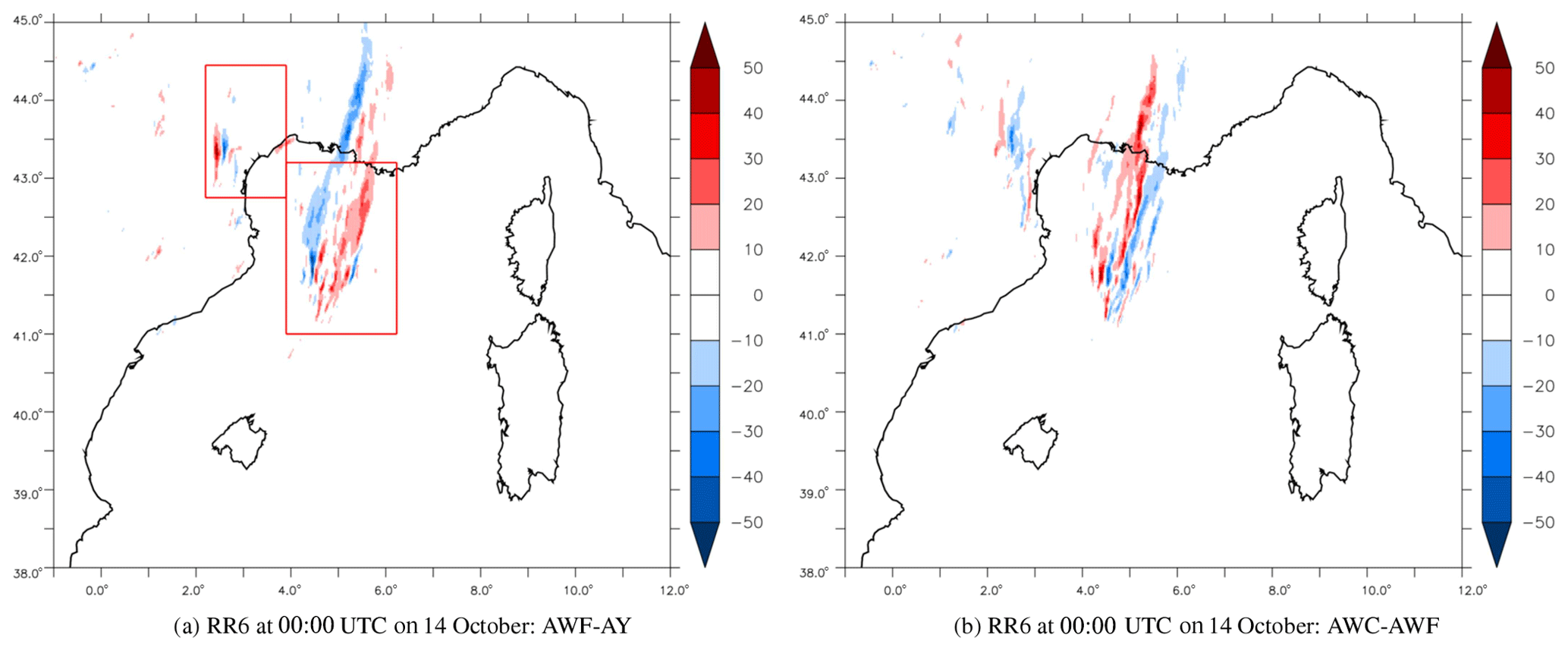
Figure 12The 6 h rainfall amount (mm) differences at 00:00 UTC on 14 October between AWF–AY (a) and AWC–AWF (b).
Figure 12 presents the differences in the 6 h rainfall amount between 18:00 UTC on 13 October and 00:00 UTC on 14 October. On average, the total amount of rainfall in the subareas in Fig. 12a, corresponding to the MCS locations, was about the same in all simulations. However, a displacement of approximately 40 km eastwards of the precipitation over the sea was found in AWF compared with AY (Fig. 12a). This displacement was directly related to the decrease in the wind speed along the French Riviera (Fig. 10c) and, thus, to the convergence line that was located further east. For the convective system over the Hérault area, only a slight shift (a few kilometres) of the maximum peak was seen. Moreover, in this area, the simulated precipitation amounts in AY and AWF were both too far inland (Fig. 4b). A slight shift of few kilometres westwards was obtained in AWC (Fig. 12b) when compared with AWF.
Thus, these differences in the precipitation forecasts highlighted the indirect impacts of taking the sea state into account: a modification of the position of the convergence line at sea related to the speed of the low-level easterly flow, followed by a small modulation of the intensity of the associated convection which was likely due to differences in term of heat fluxes upstream over the Ligurian Sea. These differences, which concern the MCS at sea, then induced low-level flow disturbances downstream in the Gulf of Lion, although with relatively little impact on the dynamics of the precipitating system that affected the Hérault area. This demonstrated that the mechanism involved in the formation of this inland system, i.e. the orographic uplift, and the reinforcement by the convergence between the southerly flow and the large-scale front, were dominant features and appeared to be less sensitive to the sea surface conditions (for the precipitating system in question).
Mediterranean HPEs are known to be violent events and are quite often associated with strong wind conditions and, thus, a very rough sea state. This study investigated the role of the representation of the sea state during the HPE that occurred between the 12 and 14 October 2016 south of France. Thanks to sensitivities experiments, the strong air–sea interactions during the event were analysed and allowed us to evaluate the impact of the representation of the sea state in the forecasting system.
For this purpose, a set of high-resolution (1.3 km) numerical simulations was realized using the AROME atmospheric model and the WW3 wave model, both in stand-alone mode or in the two-way coupled atmosphere–wave mode. To describe the turbulent fluxes that control the sea surface exchanges, the innovative WASP parametrization was used, as it is specifically designed to be used in coupled mode with a wave model and allows for the introduction of the dependency on waves by directly considering the peak period Tp in the calculation of the Charnock parameter as well as then in the surface roughness length z0.
Using observations and the reference simulation (AWF), we highlighted that the event in question was characterized by a convergence between a warm and moist southerly flow with a dry and cold easterly flow, which triggered convection over the sea. A second convective system, south of France, was initiated by an orographic uplift and was fed by the easterly flow. Both systems produced a large amount of precipitation. Three characteristic regions emerged from the analysis. First, the Balearic region was affected by weak wind and swell throughout the event. Next, the Gulf of Lion was initially located where the easterly flow was highest, producing a young sea with high Hs and strong air–sea fluxes. As the system moved eastwards with the highest wind intensity, the sea state evolved from a well-developed sea to a swell in this region. Finally, the French Riviera, was affected by a strong easterly wind throughout the event, generating a wind sea. The heat fluxes were the most intense in this latter region.
The simulation results were compared to various observations, including moored buoys for atmospheric and waves parameters (completed with Météo-France surface weather stations along the coasts for atmospheric parameters), ANTILOPE for the validation of the rainfall accumulations and altimetric data from satellites for the completion of the validation of wave parameters. On average, the simulations showed good agreement with either atmospheric or waves observations. However, it can be noticed that both Hs and Tp tended to be underestimated by the model, whereas the atmospheric parameters tended to be overestimated. Furthermore, the simulated convective system over the sea appeared to move eastwards faster than the observed system.
A sensitivity analysis was then carried out to study the impacts of waves and of the atmosphere–wave coupling. It showed large differences when the impact of the sea state was taken into account in the surface turbulent fluxes. Indeed, in AWF (compared with AY), under a strong easterly wind upstream of the convective system, the generated wind sea significantly increased the sea surface roughness length (locally up to m) and the momentum flux, which resulted in a slowdown of the 10 m wind intensity of more than 1 m s−1 over a large area. This decrease was more important than in the previous studies of Thévenot et al. (2016) and Bouin et al. (2017) due to very rough sea conditions and a strong wind regime in our study. Furthermore, a decrease in the latent heat flux was noticed along the French Riviera but did not represent a significant decrease in the total flux (by 2 % on average). Larger differences were found under the convective system but were more likely associated with differences in its location over the sea at the small scale. The scores did not show a significant change except with respect to the wind intensity; this wind intensity change was especially obvious at the Azur buoy where the wind decreased in AWF and the bias was reduced.
Looking at the impact of air–wave coupling by comparing AWC to AWF, small effects were found. As a feedback of the wind on waves, we found a decrease in Hs and Tp compared with WY resulting from the associated coupling that interactively balances the wind sea, the stress and the wind. Thus, the coupling effect appeared to be of same order as the forcing effect when compared with AY, and the comparison between WY (forcing AWF) and AWC showed very close results in terms of wave modelling. However, this result on coupling must be moderated by the fact that it was a single case study with only one configuration, and only one short-term forecast was considered. To conclude more robustly on the effect of the wave coupling, additional tests with the AROME–WW3 coupled system must be conducted regarding notably the parameterizations of the WW3 configuration, the initialization or the coupling frequency, also considering a longer forecast (or longer period of successive forecasts).
In all simulations the rainfall amount forecast was in good agreement in southern France over the Hérault area. It was found that the convective system over the sea was shifted eastwards in AWF by about 40 km compared with AY during Phase II. This was due to the changes in the low-level dynamics in AWF in response to the sea state, which modified the position of the convergence line.
Waves did not have a significant impact on heat fluxes in AWF nor in AWC, whereas there were favourable conditions including a strong sea state comprised of a young sea co-located with strong turbulent heat fluxes. Thus, it seemed that the sea state could not directly affect the heat exchanges at the air–sea interface during Mediterranean HPEs in a significant way. Nevertheless, the fact that the heat fluxes are not significantly modified in the sensitivity experiments promotes confidence in the understanding of the waves' impact, which appears to be limited to a dynamical effect that displaces the convergence and is not directly related to a large modification of the convective system intensity (see, e.g. Rainaud et al., 2017 for IOP16a and Sauvage et al., 2018a for sensitivity tests to SST or sea surface fluxes parametrization). Considering the dynamical impact appears relevant in high-resolution weather forecast, as it affected the marine low-level flow whose velocity is a key ingredient in HPE events (Bresson et al., 2012).
In conclusion, the results obtained in this study, even if they only concern one case, mark a new step in our understanding of the sea state impact on Mediterranean HPEs, after the studies of Thévenot et al. (2016) and Bouin et al. (2017), and confirm the following:
-
a slowdown of the low-level wind due to higher surface roughness, which increases the momentum flux (even in a moderate-wind context as in the studied case of Thévenot et al., 2016);
-
differences in the low-level dynamics that influence the positioning of the convergence (directly, as in this case, or indirectly as it modifies the propagation of cold pools over the sea, as in Bouin et al., 2017) and, consequently, the location of the heaviest precipitation.
The analysis of the latent and sensible heat flux sensitivity shows that there is no significant impact on the heat and moisture exchanges at the sea surface (in spite of a situation favourable to large air–wave interactions with a very strong wind regime at low-level generating a wind sea).
However, further investigations still need to be carried out in order to improve our understanding of air–sea interactions. In particular, the wave impact, in terms of sea spray, was not included here. The impact of wave interactions may also increase with time during the forecast as well as progressively from one forecast to another, as WW3 restarts each time from the previous forecast at T+24 h. However, the experimental design used here, in a deterministic framework and with the same atmospheric initiation in AWC and AWF, can not fully clarify this issue. To properly consider the growth of the wave impacts, it would be necessary to run longer experiments (more than three successive forecasts) and also to include the production of a new atmospheric analysis using the previous forecast (of AWF or AWC) as a background. Ensembles and other meteorological situations must also be considered to enlarge the evaluation of the importance of the wind–wave interactions for convection-permitting NWP models.
Future work will also consist of adding the interactive evolution of the ocean and, thus, of the sea surface temperature (constant here during the forecast time) which is known to have an effect on the lower levels of the atmosphere. This will be done using kilometric-scale tri-coupled ocean–atmosphere–wave simulations. One objective is to quantify the impact of the ocean on the forecast compared to the impact of waves. Finally, the WASP parametrization of the sea surface turbulent fluxes needs to be tested and validated on more study cases, especially during strong wind conditions, in order to further assess its added value.
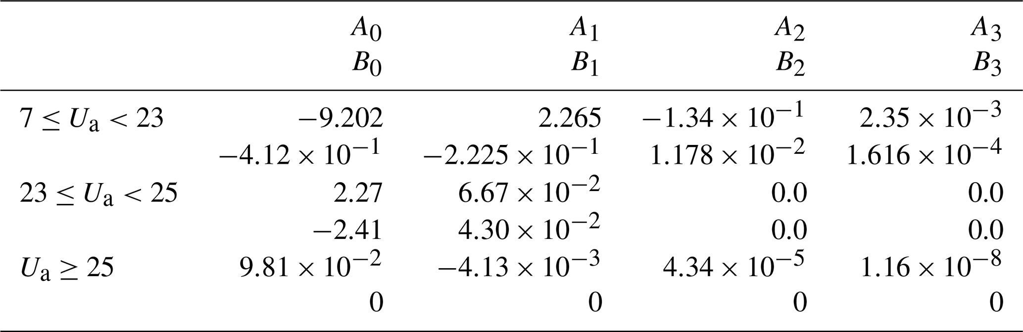
In the Wave-Age-dependant Stress Parametrization (WASP), the Charnock parameter (αch) is defined differently depending on the wind speed range, as follows:
-
first-level wind speed (Ua) below 7 m s−1 is a power of Ua: , where a=0.7 and ;
-
when Ua is above 7 m s−1, the dependency on wave age (χ) is introduced and is defined as αch=AχB, where A and B are polynomial functions of Ua.
as detailed in Table A1.
Thus, the dependency of the Charnock parameter and the decrease in the drag coefficient under very strong wind conditions are represented, and the WASP parametrization, unlike those based on wave age Charnock parameters, is suitable for very high wind speeds.
Table A1Coefficients of the polynomial functions A and B, depending on the wind speed range.
The altimeter data are freely available from the CERSAT service at Ifremer: ftp://ftp.ifremer.fr/ifremer/cersat/ (last access: 3 February 2020). The moored buoys' data and the PSY4V3R1 daily analyses were made available by the Copernicus Marine Environment Monitoring Service: http://marine.copernicus.eu/services-portfolio/access-to-products/?option=com_csw&view=details&product_id=INSITU_MED_NRT_OBSERVATIONS_013_035, http://marine.copernicus.eu/services-portfolio/access-to-products/?option=com_csw&view=details&product_id=GLOBAL_ANALYSIS_FORECAST_PHY_001_024 (last access: 3 February 2020). The moored buoys' data are also available from the HyMeX database: https://mistrals.sedoo.fr/HyMeX/ (last access: 3 February 2020). Météo France surface weather stations around the Mediterranean Sea are also available on HyMeX database (Brissebat, 2016). The Météo-France ANTILOPE product is available on demand for research purposes (upon request to olivier.laurantin@meteo.fr). The source codes are available online (WaveWatchIII at https://polar.ncep.noaa.gov/waves/wavewatch/; OASIS at https://portal.enes.org/oasis; and SURFEX at http://www.umr-cnrm.fr/surfex/; last access: 3 February 2020), although the operational AROME code cannot be obtained. The WASP parametrization will be included in the next release (v9) of SURFEX, but it can be provided on demand from the authors for older SURFEX versions (back to v7_3). The simulation results can be obtained upon request from the authors.
All authors (CS, CLB, MNB and VD) contributed to the conceptualization and methodology of the study as well as drafting, reviewing and editing the article. MNB developed the WASP parametrization and managed its integration into the SURFEX code. The coupling development and simulations were undertaken by CS and CLB. CS, CLB and MNB carried out the validation and analysis of the results.
The authors declare that they have no conflict of interest.
This article is part of the special issue “Hydrological cycle in the Mediterranean (ACP/AMT/GMD/HESS/NHESS/OS inter-journal SI)”. It is not associated with a conference.
This work is a contribution to the HyMeX programme (Hydrological cycle in the Mediterranean EXperiment – http://www.hymex.org, last access: 3 February 2020) and is supported by INSU-MISTRALS. The authors acknowledge the Occitanie region, France, for its contribution to César Sauvage's PhD at CNRM. The authors acknowledge the MISTRALS/HyMeX database teams (ESPRI/IPSL and SEDOO/OMP) for their help with accessing the surface weather station data. The authors gratefully acknowledge Mickaël Accensi and Fabrice Ardhuin (LOPS) for their invaluable help and advice concerning the development and application of the north-western Mediterranean configuration of the WaveWatch III model. Finally, the authors wish to thank Olivier Nuissier (CNRM) for discussions regarding the characteristics of the Mediterranean heavy precipitation event that was studied.
This research has been supported by the Région Occitanie France (AAP allocation doctorale 2016 grant no. 15066459) and the CNRS/INSU MISTRALS/HyMeX (grant no. MISTRALS/HyMeX).
This paper was edited by Heini Wernli and reviewed by two anonymous referees.
Andreas, E. L.: Sea Spray and the Turbulent Air-Sea Heat Fluxes, J. Geophys. Res., 97, 11429–11441, https://doi.org/10.1029/92jc00876, 1992. a
Andreas, E. L., Edson, J. B., Monahan, E. C., Rouault, M. P., and Smith, S. D.: The spray contribution to net evaporation from the sea: A review of recent progress, Bound.-Lay. Meteorol., 72, 3–52, https://doi.org/10.1007/bf00712389, 1995. a
Ardhuin, F. and Roland, A.: Coastal wave reflection, directional spread, and seismoacoustic noise sources, J. Geophys. Res.-Ocean., 117, C00J20, https://doi.org/10.1029/2011JC007832, 2012. a
Ardhuin, F., O'Reilly, W. C., Herbers, T. H. C., and Jessen, P. F.: Swell Transformation across the Continental Shelf, Part I: Attenuation and Directional Broadening, J. Phys. Oceanogr., 33, 1921–1939, https://doi.org/10.1175/1520-0485(2003)033<1921:STATCS>2.0.CO;2, 2003. a
Ardhuin, F., Chapron, B., and Collard, F.: Observation of swell dissipation across oceans, Geophys. Res. Lett., 36, L06607, https://doi.org/10.1029/2008gl037030, 2009. a
Ardhuin, F., Rogers, E., Babanin, A. V., Filipot, J.-F., Magne, R., Roland, A., van der Westhuysen, A., Queffeulou, P., Lefevre, J.-M., Aouf, L., and Collard, F.: Semiempirical Dissipation Source Functions for Ocean Waves, Part I: Definition, Calibration, and Validation, J. Phys. Oceanogr., 40, 1917–1941, https://doi.org/10.1175/2010JPO4324.1, 2010. a
Ardhuin, F., Stopa, J. E., Chapron, B., Collard, F., Husson, R., Jensen, R. E., Johannessen, J., Mouche, A., Passaro, M., Quartly, G. D., Swail, V., and Young, I.: Observing Sea States, Front. Marine Sci., 6, 29 pp., https://doi.org/10.3389/fmars.2019.00124, 2019. a
Bao, J.-W., Wilczak, J. M., Choi, J.-K., and Kantha, L. H.: Numerical Simulations of Air-Sea Interaction under High Wind Conditions Using a Coupled Model: A Study of Hurricane Development, Mon. Weather Rev., 128, 2190–2210, https://doi.org/10.1175/1520-0493(2000)128<2190:nsoasi>2.0.co;2, 2000. a
Bao, J.-W., Fairall, C. W., Michelson, S. A., and Bianco, L.: Parameterizations of Sea-Spray Impact on the Air-Sea Momentum and Heat Fluxes, Mon. Weather Rev., 139, 3781–3797, https://doi.org/10.1175/mwr-d-11-00007.1, 2011. a
Battjes, J. and Janssen, J.: Energy loss and set-up due to breaking of random waves, Coast. Eng. Proceed., 1, available at: https://journals.tdl.org/icce/index.php/icce/article/view/3294 (last access: 3 February 2020), 1978. a
Beljaars, A. C. M.: The parametrization of surface fluxes in large-scale models under free convection, Q. J. Roy. Meteor. Soc., 121, 255–270, https://doi.org/10.1002/qj.49712152203, 1994. a
Bianco, L., Bao, J.-W., Fairall, C. W., and Michelson, S. A.: Impact of Sea-Spray on the Atmospheric Surface Layer, Bound.-Lay. Meteorol., 140, 361–381, https://doi.org/10.1007/s10546-011-9617-1, 2011. a
Bouin, M.-N., Redelsperger, J.-L., and Lebeaupin Brossier, C.: Processes leading to deep convection and sensitivity to sea-state representation during HyMeX IOP8 heavy precipitation event, Q. J. Roy. Meteor. Soc., 143, 2600–2615, https://doi.org/10.1002/qj.3111, 2017. a, b, c, d, e
Bouin, M. N. and Emzivat, G.: Buoys, HyMeX, available at: https://mistrals.sedoo.fr/HyMeX, last access: 3 February 2020.
Bresson, E., Ducrocq, V., Nuissier, O., Ricard, D., and de Saint‐Aubin C.: Idealized numerical simulations of quasi‐stationary convective systems over the Northwestern Mediterranean complex terrain, Q. J. Roy. Meteor. Soc., 138, 1751–1763, 2012. a
Brissebat, G.: Operational surface weather observation stations over France – Hourly data, available at: https://mistrals.sedoo.fr/HyMeX (last access: 3 February 2020), 2016.
Businger, J. A., Wyngaard, J. C., Izumi, Y., and Bradley, E. F.: Flux-Profile Relationships in the Atmospheric Surface Layer, J. Atmos. Sci., 28, 181–189, https://doi.org/10.1175/1520-0469(1971)028<0181:fprita>2.0.co;2, 1971. a
Cassola, F., Ferrari, F., Mazzino, A., and Miglietta, M. M.: The role of the sea on the flash floods events over Liguria (northwestern Italy), Geophys. Res. Lett., 43, 3534–3542, https://doi.org/10.1002/2016gl068265, 2016. a
CERFACS, CNRM: OASIS coupler, available at: https://portal.enes.org/oasis, last access: 3 February 2020.
CERSAT: Satellite data, Ifremer, available at: ftp://ftp.ifremer.fr/ifremer/cersat/, last access: 3 February 2020.
Charnock, H.: Wind stress on a water surface, Q. J. Roy. Meteor. Soc., 81, 639–640, https://doi.org/10.1002/qj.49708135027, 1955. a, b
CMEMS – Global Monitoring and Forecasting Centre: INSITU_MED_NRT_OBSERVATIONS_013_035, available at: http://marine.copernicus.eu/services-portfolio/access-to-products/?option=com_csw&view=details&product_id=INSITU_MED_NRT_OBSERVATIONS_013_035, last access: 3 February 2020.
CMEMS – Global Monitoring and Forecasting Centre: GLOBAL_ANALYSIS_FORECAST_PHY_001_024, available at: http://marine.copernicus.eu/services-portfolio/access-to-products/?option=com_csw&view=details&product_id=GLOBAL_ANALYSIS_FORECAST_PHY_001_024, last access: 3 February 2020.
CNRM, Météo-France: SURFEX, available at: http://www.umr-cnrm.fr/surfex/, last access: 3 February 2020.
Courtier, P., Freydier, C., Geleyn, J.-F., Rabier, F., and Rochas, M.: The Arpege project at Meteo France, in: Seminar on Numerical Methods in Atmospheric Models, 9–13 September 1991, Vol. II, ECMWF, ECMWF, Shinfield Park, Reading, 193–232, available at: https://www.ecmwf.int/node/8798 (last access: 3 February 2020), 1991. a
Craig, A., Valcke, S., and Coquart, L.: Development and performance of a new version of the OASIS coupler, OASIS3-MCT_3.0, Geosci. Model Dev., 10, 3297–3308, https://doi.org/10.5194/gmd-10-3297-2017, 2017. a
Cuxart, J., Bougeault, P., and Redelsperger, J.-L.: A turbulence scheme allowing for mesoscale and large-eddy simulations, Q. J. Roy. Meteor. Soc., 126, 1–30, https://doi.org/10.1002/qj.49712656202, 2000. a
Delrieu, G., Nicol, J., Yates, E., Kirstetter, P.-E., Creutin, J.-D., Anquetin, S., Obled, C., Saulnier, G.-M., Ducrocq, V., Gaume, E., Payrastre, O., Andrieu, H., Ayral, P.-A., Bouvier, C., Neppel, L., Livet, M., Lang, M., du Châtelet, J. P., Walpersdorf, A., and Wobrock, W.: The Catastrophic Flash-Flood Event of 8–9 September 2002 in the Gard Region, France: A First Case Study for the Cévennes–Vivarais Mediterranean Hydrometeorological Observatory, J. Hydrometeorol., 6, 34–52, https://doi.org/10.1175/JHM-400.1, 2005. a
Donelan, M. A.: Air-sea interaction, The Sea, 9, 239–292, 1990. a
Donelan, M. A., Dobson, F. W., Smith, S. D., and Anderson, R. J.: On the Dependence of Sea Surface Roughness on Wave Development, J. Phys. Oceanogr., 23, 2143–2149, https://doi.org/10.1175/1520-0485(1993)023<2143:OTDOSS>2.0.CO;2, 1993. a
Doyle, J. D.: Coupled ocean wave/atmosphere mesoscale model simulations of cyclogenesis, Tellus A, 47, 766–778, https://doi.org/10.3402/tellusa.v47i5.11574, 1995. a
Doyle, J. D.: Coupled Atmosphere-Ocean Wave Simulations under High Wind Conditions, Mon. Weather Rev., 130, 3087–3099, https://doi.org/10.1175/1520-0493(2002)130<3087:caowsu>2.0.co;2, 2002. a
Drennan, W. M., Graber, H. C., Hauser, D., and Quentin, C.: On the wave age dependence of wind stress over pure wind seas, J. Geophys. Res.-Ocean., 108, 8062, https://doi.org/10.1029/2000JC000715, 2003. a
Drennan, W. M., Taylor, P. K., and Yelland, M. J.: Parameterizing the Sea Surface Roughness, J. Phys. Oceanogr., 35, 835–848, https://doi.org/10.1175/jpo2704.1, 2005. a
Ducrocq, V., Nuissier, O., Ricard, D., Lebeaupin, C., and Thouvenin, T.: A numerical study of three catastrophic precipitating events over southern France, Part II: Mesoscale triggering and stationarity factors, Q. J. Roy. Meteor. Soc., 134, 131–145, https://doi.org/10.1002/qj.199, 2008. a
Ducrocq, V., Davolio, S., Ferretti, R., Flamant, C., Santaner, V. H., Kalthoff, N., Richard, E., and Wernli, H.: Introduction to the HyMeX Special Issue on “Advances in understanding and forecasting of heavy precipitation in the Mediterranean through the HyMeX SOP1 field campaign”, Q. J. Roy. Meteor. Soc., 142, 1–6, https://doi.org/10.1002/qj.2856, 2016. a
Duffourg, F. and Ducrocq, V.: Origin of the moisture feeding the Heavy Precipitating Systems over Southeastern France, Nat. Hazards Earth Syst. Sci., 11, 1163-1178, https://doi.org/10.5194/nhess-11-1163-2011, 2011. a
Duffourg, F., Nuissier, O., Ducrocq, V., Flamant, C., Chazette, P., Delanoë, J., Doerenbecher, A., Fourrié, N., Di Girolamo, P., Lac, C., Legain, D., Martinet, M., Said, F., and Bock, O.: Offshore deep convection initiation and maintenance during the HyMeX IOP 16a heavy precipitation event, Q. J. Roy. Meteor. Soc., 142, 259–274, https://doi.org/10.1002/qj.2725, 2016. a
Edson, J. B., Jampana, V., Weller, R. A., Bigorre, S. P., Plueddemann, A. J., Fairall, C. W., Miller, S. D., Mahrt, L., Vickers, D., and Hersbach, H.: On the Exchange of Momentum over the Open Ocean, J. Phys. Oceanogr., 43, 1589–1610, https://doi.org/10.1175/jpo-d-12-0173.1, 2013. a
Fairall, C. W., Bradley, E. F., Rogers, D. P., Edson, J. B., and Young, G. S.: Bulk parameterization of air-sea fluxes for Tropical Ocean-Global Atmosphere Coupled-Ocean Atmosphere Response Experiment (TOGA-COARE), J. Geophys. Res.-Ocean., 101, 3747–3764, https://doi.org/10.1029/95jc03205, 1996. a
Fairall, C. W., Bradley, E. F., Hare, J. E., Grachev, A. A., and Edson, J. B.: Bulk Parameterization of Air–Sea Fluxes: Updates and Verification for the COARE Algorithm, J. Clim., 16, 571–591, https://doi.org/10.1175/1520-0442(2003)016<0571:BPOASF>2.0.CO;2, 2003. a, b
Garg, N., Ng, E. Y. K., and Narasimalu, S.: The effects of sea spray and atmosphere – wave coupling on air – sea exchange during a tropical cyclone, Atmos. Chem. Phys., 18, 6001–6021, https://doi.org/10.5194/acp-18-6001-2018, 2018. a
Hasselmann, S., Hasselmann, K., Allender, J. H., and Barnett, T. P.: Computations and Parameterizations of the Nonlinear Energy Transfer in a Gravity-Wave Specturm, Part II: Parameterizations of the Nonlinear Energy Transfer for Application in Wave Models, J. Phys. Oceanogr., 15, 1378–1391, https://doi.org/10.1175/1520-0485(1985)015<1378:CAPOTN>2.0.CO;2, 1985. a
Janssen, P.: The Interaction of Ocean Waves and Wind, Cambridge University Press, https://doi.org/10.1017/cbo9780511525018, 2004. a
Janssen, P., Doyle, J., Bidlot, J.-R., Hansen, B., Isaksen, L., and Viterbo, P.: Impact and feedback of ocean waves on the atmosphere, ECMWF Technical Memoranda Series, 32 pp., https://doi.org/10.21957/c1ey8zifx, 2001. a
Janssen, P. A. E. M.: Wave-Induced Stress and the Drag of Air Flow over Sea Waves, J. Phys. Oceanogr., 19, 745–754, https://doi.org/10.1175/1520-0485(1989)019<0745:wisatd>2.0.co;2, 1989. a
Janssen, P. A. E. M.: Quasi-linear Theory of Wind-Wave Generation Applied to Wave Forecasting, J. Phys. Oceanogr., 21, 1631–1642, https://doi.org/10.1175/1520-0485(1991)021<1631:qltoww>2.0.co;2, 1991. a, b
Janssen, P. A. E. M.: Experimental Evidence of the Effect of Surface Waves on the Airflow, J. Phys. Oceanogr., 22, 1600–1604, https://doi.org/10.1175/1520-0485(1992)022<1600:eeoteo>2.0.co;2, 1992. a
Kain, J. S. and Fritsch, J. M.: A One-Dimensional Entraining/Detraining Plume Model and Its Application in Convective Parameterization, J. Atmos. Sci., 47, 2784–2802, https://doi.org/10.1175/1520-0469(1990)047<2784:AODEPM>2.0.CO;2, 1990. a
Katsafados, P., Papadopoulos, A., Korres, G., and Varlas, G.: A fully coupled atmosphere–ocean wave modeling system for the Mediterranean Sea: interactions and sensitivity to the resolved scales and mechanisms, Geosci. Model Dev., 9, 161–173, https://doi.org/10.5194/gmd-9-161-2016, 2016. a
Kepert, J., Fairall, C., and Bao, J.-W.: Modelling the Interaction Between the Atmospheric Boundary Layer and Evaporating Sea Spray Droplets, in: Atmospheric and Oceanographic Sciences Library, Springer Netherlands, 363–409, https://doi.org/10.1007/978-94-015-9291-8_14, 1999. a
Laurantin, O.: ANTILOPE: Hourly rainfall analysis merging radar and rain gauge data, Proceedings of Weather Radar and Hydrology Conference 2008, 2008. a
Lebeaupin Brossier, C., Ducrocq, V., and Giordani, H.: Sensitivity of torrential rain events to the sea surface temperature based on high-resolution numerical forecasts, J. Geophys. Res.-Atmos., 111, D12110, https://doi.org/10.1029/2005JD006541, d12110, 2006. a
Lebeaupin Brossier, C., Ducrocq, V., and Giordani, H.: Sensitivity of three Mediterranean heavy rain events to two different sea surface fluxes parameterizations in high-resolution numerical modeling, J. Geophys. Res.-Atmos., 113, d21109, https://doi.org/10.1029/2007JD009613, 2008. a
Lellouche, J.-M., Le Galloudec, O., Drévillon, M., Régnier, C., Greiner, E., Garric, G., Ferry, N., Desportes, C., Testut, C.-E., Bricaud, C., Bourdallé-Badie, R., Tranchant, B., Benkiran, M., Drillet, Y., Daudin, A., and De Nicola, C.: Evaluation of global monitoring and forecasting systems at Mercator Océan, Ocean Sci., 9, 57–81, https://doi.org/10.5194/os-9-57-2013, 2013. a
Llasat, M. C., Llasat-Botija, M., Petrucci, O., Pasqua, A. A., Rosselló, J., Vinet, F., and Boissier, L.: Towards a database on societal impact of Mediterranean floods within the framework of the HYMEX project, Nat. Hazards Earth Syst. Sci., 13, 1337–1350, https://doi.org/10.5194/nhess-13-1337-2013, 2013. a
Mahrt, L., Vickers, D., Sun, J., Jensen, N. O., Jørgensen, H., Pardyjak, E., and Fernando, H.: Determination Of The Surface Drag Coefficient, Bound.-Lay. Meteorol., 99, 249–276, https://doi.org/10.1023/a:1018915228170, 2001. a
Masson, V.: A Physically-Based Scheme For The Urban Energy Budget In Atmospheric Models, Bound.-Lay. Meteorol., 94, 357–397, https://doi.org/10.1023/A:1002463829265, 2000. a
Masson, V., Le Moigne, P., Martin, E., Faroux, S., Alias, A., Alkama, R., Belamari, S., Barbu, A., Boone, A., Bouyssel, F., Brousseau, P., Brun, E., Calvet, J.-C., Carrer, D., Decharme, B., Delire, C., Donier, S., Essaouini, K., Gibelin, A.-L., Giordani, H., Habets, F., Jidane, M., Kerdraon, G., Kourzeneva, E., Lafaysse, M., Lafont, S., Lebeaupin Brossier, C., Lemonsu, A., Mahfouf, J.-F., Marguinaud, P., Mokhtari, M., Morin, S., Pigeon, G., Salgado, R., Seity, Y., Taillefer, F., Tanguy, G., Tulet, P., Vincendon, B., Vionnet, V., and Voldoire, A.: The SURFEXv7.2 land and ocean surface platform for coupled or offline simulation of earth surface variables and fluxes, Geosci. Model Dev., 6, 929–960, https://doi.org/10.5194/gmd-6-929-2013, 2013. a
Meroni, A. N., Parodi, A., and Pasquero, C.: Role of SST Patterns on Surface Wind Modulation of a Heavy Midlatitude Precipitation Event, J. Geophys. Res.-Atmos., 123, 9081–9096, https://doi.org/10.1029/2018jd028276, 2018. a
Moon, I.-J., Ginis, I., and Hara, T.: Effect of Surface Waves on Air–Sea Momentum Exchange, Part II: Behavior of Drag Coefficient under Tropical Cyclones, J. Atmos. Sci., 61, 2334–2348, https://doi.org/10.1175/1520-0469(2004)061<2334:EOSWOA>2.0.CO;2, 2004. a
NOAA: WaveWatch 3 wave model, available at: https://polar.ncep.noaa.gov/waves/wavewatch/, last access: 3 February 2020.
Noilhan, J. and Planton, S.: A Simple Parameterization of Land Surface Processes for Meteorological Models, Mon. Weather Rev., 117, 536–549, 1989. a
Nuissier, O., Joly, B., Joly, A., Ducrocq, V., and Arbogast, P.: A statistical downscaling to identify the large‐scale circulation patterns associated with heavy precipitation events over southern France, Q. J. Roy. Meteor. Soc., 137, 1812–1827, https://doi.org/10.1002/qj.866, 2011. a, b
Oost, W., Komen, G., Jacobs, C., and Oort, C. V.: New evidence for a relation between wind stress and wave age from measurements during ASGAMAGE, Bound.-Lay. Meteorol., 103, 409–438, https://doi.org/10.1023/a:1014913624535, 2002. a, b, c, d
OSTM/Jason-2 Products Handbook: OSTM/Jason-2 Products Handbook, CNES: SALP-MU-M-OP-15815-CN, Ed 1.2, 2008. a
Pineau-Guillou, L., Ardhuin, F., Bouin, M.-N., Redelsperger, J.-L., Chapron, B., Bidlot, J.-R., and Quilfen, Y.: Strong winds in a coupled wave–atmosphere model during a North Atlantic storm event: evaluation against observations, Q. J. Roy. Meteor. Soc., 144, 317–332, https://doi.org/10.1002/qj.3205, 2018. a, b
Pinty, J.-P. and Jabouille, P.: A mixed-phase cloud parameterization for use in mesoscale non-hydrostatic model: simulations of a squall line and of orographic precipitations, Conf. on Cloud Physics, Am. Meteorol. Soc., 217–220, 1998. a
Powell, M. D., Vickery, P. J., and Reinhold, T. A.: Reduced drag coefficient for high wind speeds in tropical cyclones, Nature, 422, 279–283, https://doi.org/10.1038/nature01481, 2003. a
Rainaud, R., Lebeaupin Brossier, C., Ducrocq, V., and Giordani, H.: High-resolution air–sea coupling impact on two heavy precipitation events in the Western Mediterranean, Q. J. Roy. Meteor. Soc., 143, 2448–2462, https://doi.org/10.1002/qj.3098, 2017. a
Rascle, N. and Ardhuin, F.: A global wave parameter database for geophysical applications, Part 2: Model validation with improved source term parameterization, Ocean Modell., 70, 174–188, https://doi.org/10.1016/j.ocemod.2012.12.001, 2013. a
Renault, L., Chiggiato, J., Warner, J. C., Gomez, M., Vizoso, G., and Tintoré, J.: Coupled atmosphere-ocean-wave simulations of a storm event over the Gulf of Lion and Balearic Sea, J. Geophys. Res.-Ocean., 117, C09019, https://doi.org/10.1029/2012JC007924, c09019, 2012. a
Ricchi, A., Miglietta, M. M., Falco, P. P., Benetazzo, A., Bonaldo, D., Bergamasco, A., Sclavo, M., and Carniel, S.: On the use of a coupled ocean–atmosphere–wave model during an extreme cold air outbreak over the Adriatic Sea, Atmos. Res., 172/173, 48–65, https://doi.org/10.1016/j.atmosres.2015.12.023, 2016. a
Rizza, U., Canepa, E., Ricchi, A., Bonaldo, D., Carniel, S., Morichetti, M., Passerini, G., Santiloni, L., Puhales, F. S., and Miglietta, M.: Influence of Wave State and Sea Spray on the Roughness Length: Feedback on Medicanes, Atmosphere, 9, p. 301, https://doi.org/10.3390/atmos9080301, 2018. a
SARAL/AltiKa Products handbook: SARAL/AltiKa Products handbook, CNES: SALP-MU-M-OP-15984-CN, Issue 2, rev 3, 2013. a
Sauvage, C., Brossier, C. L., Bouin, M.-N., and Ducrocq, V.: Role of the sea state on the air-sea exchanges during a Mediterranean heavy precipitation event in a kilometer-scale forecast system, Preprints, 21st AMS Conf. on Air-Sea Interaction, Oklahoma city, OK, p. 6, https://ams.confex.com/ams/23BLT21ASI/mediafile/Manuscript/Paper345111/Extended_Abstract_AMS.pdf (last access: 3 February 2020), 2018a. a, b
Sauvage, C., Brossier, C. L., Ducrocq, V., Bouin, M.-N., Vincendon, B., Verdecchia, M., Taupier-Letage, I., and Orain, F.: Impact of the representation of the freshwater river input in the Western Mediterranean Sea, Ocean Modell., 131, 115–131, https://doi.org/10.1016/j.ocemod.2018.09.005, 2018b. a
Seity, Y., Brousseau, P., Malardel, S., Hello, G., Bénard, P., Bouttier, F., Lac, C., and Masson, V.: The AROME-France convective scale operational model, Mon. Weather Rev., 139, 976–991, 2011. a
Smith, S. D., Anderson, R. J., Oost, W. A., Kraan, C., Maat, N., Cosmo, J. D., Katsaros, K. B., Davidson, K. L., Bumke, K., Hasse, L., and Chadwick, H. M.: Sea surface wind stress and drag coefficients: The HEXOS results, Bound.-Lay. Meteorol., 60, 109–142, https://doi.org/10.1007/bf00122064, 1992. a
Stocchi, P. and Davolio, S.: Intense air-sea exchange and heavy rainfall: impact of the northern Adriatic SST, Adv. Sci. Res., 13, 7–12, https://doi.org/10.5194/asr-13-7-2016, 2017. a
Strajnar, B., Cedilnik, J., Fettich, A., Ličer, M., Pristov, N., Smerkol, P., and Jerman, J.: Impact of two-way coupling and sea-surface temperature on precipitation forecasts in regional atmosphere and ocean models, Q. J. Roy. Meteor. Soc., 145, 228–242, https://doi.org/10.1002/qj.3425, 2019. a
Taylor, P. K. and Yelland, M. J.: The Dependence of Sea Surface Roughness on the Height and Steepness of the Waves, J. Phys. Oceanogr., 31, 572–590, https://doi.org/10.1175/1520-0485(2001)031<0572:tdossr>2.0.co;2, 2001. a
Thévenot, O., Bouin, M.-N., Ducrocq, V., Lebeaupin Brossier, C., Nuissier, O., Pianezze, J., and Duffourg, F.: Influence of the sea state on Mediterranean heavy precipitation: a case-study from HyMeX SOP1, Q. J. Roy. Meteor. Soc., 142, 377–389, https://doi.org/10.1002/qj.2660, 2016. a, b, c, d, e
The WAVEWATCH III Development Group: User manual and system documentation of WAVEWATCH III version 5.16, Tech. Note 329, 2016. a
Tolman, H. L.: Effects of Numerics on the Physics in a Third-Generation Wind-Wave Model, J. Phys. Oceanogr., 22, 1095–1111, https://doi.org/10.1175/1520-0485(1992)022<1095:EONOTP>2.0.CO;2, 1992. a
Varlas, G., Katsafados, P., Papadopoulos, A., and Korres, G.: Implementation of a two-way coupled atmosphere-ocean wave modeling system for assessing air-sea interaction over the Mediterranean Sea, Atmos. Res., 208, 201–217, https://doi.org/10.1016/j.atmosres.2017.08.019, 2018. a, b
Voldoire, A., Decharme, B., Pianezze, J., Lebeaupin Brossier, C., Sevault, F., Seyfried, L., Garnier, V., Bielli, S., Valcke, S., Alias, A., Accensi, M., Ardhuin, F., Bouin, M.-N., Ducrocq, V., Faroux, S., Giordani, H., Léger, F., Marsaleix, P., Rainaud, R., Redelsperger, J.-L., Richard, E., and Riette, S.: SURFEX v8.0 interface with OASIS3-MCT to couple atmosphere with hydrology, ocean, waves and sea-ice models, from coastal to global scales, Geosci. Model Dev., 10, 4207–4227, https://doi.org/10.5194/gmd-10-4207-2017, 2017. a
Wahle, K., Staneva, J., Koch, W., Fenoglio-Marc, L., Ho-Hagemann, H. T. M., and Stanev, E. V.: An atmosphere–wave regional coupled model: improving predictions of wave heights and surface winds in the southern North Sea, Ocean Sci., 13, 289–301, https://doi.org/10.5194/os-13-289-2017, 2017. a
- Abstract
- Introduction
- Numerical set-up
- Validation of the experiments
- Event description
- Sensitivity analysis
- Conclusions
- Appendix A: Charnock parameter in WASP
- Data availability
- Author contributions
- Competing interests
- Special issue statement
- Acknowledgements
- Financial support
- Review statement
- References