Evaluation of aerosol and cloud properties in three climate models using MODIS observations and its corresponding COSP simulator, as well as their application in aerosol–cloud interactions

The evaluation of modelling diagnostics with appropriate observations is an important task that establishes the capabilities and reliability of models. In this study we compare aerosol and cloud properties obtained from three different climate models (ECHAM-HAM, ECHAM-HAM-SALSA, and NorESM) with satellite observations using Moderate Resolution Imaging Spectroradiometer (MODIS) data. The simulator MODIS-COSP version 1.4 was implemented into the climate models to obtain MODIS-like cloud diagnostics, thus enabling model-to-model and model-to-satellite comparisons. Cloud droplet number concentrations (CDNCs) are derived identically from MODIS-COSP-simulated and MODIS-retrieved values of cloud optical depth and effective radius. For CDNC, the models capture the observed spatial distribution of higher values typically found near the coasts, downwind of the major continents, and lower values over the remote ocean and land areas. However, the COSP-simulated CDNC values are higher than those observed, whilst the direct model CDNC output is significantly lower than the MODIS-COSP diagnostics. NorESM produces large spatial biases for ice cloud properties and thick clouds over land. Despite having identical cloud modules, ECHAM-HAM and ECHAM-HAM-SALSA diverge in their representation of spatial and vertical distributions of clouds. From the spatial distributions of aerosol optical depth (AOD) and aerosol index (AI), we find that NorESM shows large biases for AOD over bright land surfaces, while discrepancies between ECHAM-HAM and ECHAM-HAM-SALSA can be observed mainly over oceans. Overall, the AIs from the different models are in good agreement globally, with higher negative biases in the Northern Hemisphere. We evaluate the aerosol–cloud interactions by computing the sensitivity parameter ACI${}_{\mathrm{CDNC}}=\mathrm{d}\ln \left(\text{CDNC}\right)/\mathrm{d}\ln \left(\text{AI}\right)$ on a global scale. However, 1 year of data may be considered not enough to assess the similarity or dissimilarities of the models due to large temporal variability in cloud properties. This study shows how simulators facilitate the evaluation of cloud properties and expose model deficiencies, which are necessary steps to further improve the parameterisation in climate models.

1 Introduction

A climate model is a powerful tool for investigating the response of the climate system to various forcings, enabling climate forecasts on seasonal to decadal timescales, and therefore it can be used for estimating projections of the future climate over the coming centuries based on future greenhouse gas and aerosol forcing scenarios (Flato, 2011). Based on physical principles, climate models reproduce many key aspects of the observed climate and aid in the understanding of the dynamics of the physical components of the climate systems.

The evaluation of modelling diagnostics is an important task that establishes the capabilities and reliability of models. When key properties of the atmosphere (e.g. clouds, aerosols) are considered, the model assessment is relevant to ensure that the climate model correctly captures key features of the climate system. The interest in the reliability of climate models reaches outside the scientific community, as these simulations will form the basis for future climate assessments and negotiations. Therefore, understanding the level of reliability is a necessary step to strengthen the robustness of climate projections and, if necessary, improve the model parameterisations for the relevant processes.

For the evaluation of parameterisations of aerosol indirect effects in global models, satellite data have been proven to be useful (Quaas et al., 2009; Boucher et al., 2013) as they provide large spatial coverage at suitable temporal resolution. Satellite instruments measure the intensity of radiation coming from a particular direction in a selected wavelength range. From the observed radiances, the geophysical quantities are then inferred by inverse modelling using a retrieval algorithm.

The compensation of modelling errors, the intrinsic uncertainties in observational data, and the possible discrepant definitions of variables between models and observational data are major issues affecting the crucial task of model evaluation. For that, satellite simulators have been developed to mimic the retrieval of observational data and to avoid ambiguities in the definition of variables mentioned above. Simulators recreate what the satellite would retrieve when observing the modelled atmosphere. By reprocessing model fields using radiative transfer calculations, they generate physical quantities fully consistent with the satellite retrievals. By including microphysical assumptions, which usually differ between models, inconsistencies in the simulators are avoided. Hence, simulators represent a robust and consistent approach not only for the application of satellite data to evaluate models but also for model-to-model comparisons. Simulators have been widely used, and their implementation in several models enables intercomparison studies on atmospheric variables, such as clouds, aerosols (Quaas et al., 2009; Williams and Bodas-Salcedo, 2017; Zhang et al., 2010; Luo et al., 2017), and upper atmospheric humidity (Bodas-Salcedo et al., 2011).

Two prominent examples of simulators are the simulator developed as part of the International Satellite Cloud Climatology Project, ISCCP, (Klein and Webb, 2009; Yu et al., 1996) and the CFMIP (Cloud Feedback Model Intercomparison Project) Observation Simulator Package, COSP (Bodas-Salcedo et al., 2011). CFMIP is part of the Coupled Model Intercomparison Project (CMIP) (Eyring et al., 2016b; Webb et al., 2017), which is a framework providing the modelling community with guidelines for the development, tuning, and evaluation of models (Eyring et al., 2016a, c). COSP is a software tool developed within the CFMIP (Webb et al., 2017), which extracts parameters for several spaceborne active sensors, such as the Cloud-Aerosol LIdar with Orthogonal Polarization (CALIOP) and the Cloud Profiling Radar (CPR), as well as for passive sensors, such as the Multi-angle Imaging SpectroRadiometer (MISR) and the Moderate Resolution Imaging Spectroradiometer (MODIS).

In this study COSP version 1.4 was implemented in three climate models, namely ECHAM-HAM, ECHAM-HAM-SALSA, and NorESM, and the diagnostic outputs of the MODIS simulator were compared to MODIS observational data collected during the year 2008. The main goal of this study is to evaluate the model's capability to realistically represent clouds by employing MODIS satellite observations and its corresponding COSP simulator. A secondary goal of the study is to estimate the aerosol–cloud interactions through the application of the cloud droplet number concentration (CDNC) derived from observed and COSP simulated values of cloud optical thickness and effective radius. Aerosol–cloud interactions are based on the role of aerosol particles in changing cloud properties, which involves several processes (Bellouin et al., 2020). In this study we focus on one of these processes, known as the first aerosol indirect effects or Twomey effect, which can be quantified by an indicator parameter, called ACI, defined as the change in an observable cloud property (e.g. cloud optical depth, cloud effective radius, cloud droplet number concentration) to a change in a cloud condensation nuclei proxy (e.g. aerosol optical depth, aerosol index, or aerosol particle number concentration). The analysis of aerosol–cloud interactions has been reported in literature by a variety of methods: studies presenting results from global scales (Feingold et al., 2001; Quaas et al., 2010) to regional scales (e.g. Saponaro et al., 2017; Ban-Weiss et al., 2014; Liu et al., 2017, 2018) and in situ observations (e.g. Sporre et al., 2014), using different approaches, i.e. observations from satellites, airborne and ground-based instrumentation, or modelling. Nonetheless, the quantification of the aerosol–cloud interactions is still a major uncertainty in understanding climate change (e.g. Lohmann et al., 2007; Quaas et al., 2009; Storelvmo, 2012; Flato et al., 2013; Lee et al., 2016; Seinfeld et al., 2016; Bellouin et al., 2020).

The choice of observations and spatial scale of a study presents intrinsic uncertainties when quantifying aerosol–cloud interactions, and some of them relate to spatial or temporal limitations or artefacts (McComiskey and Feingold, 2012). When considering satellite observations, cloud and aerosol properties are provided at a quite comprehensive spatial and temporal coverage; however, several aspects bring challenges in the analysis of these observations. The primary artefacts known to affect satellite estimation of aerosol–cloud interactions are related to (1) the inability to untangling aerosol and cloud retrievals from meteorology (e.g. aerosol humidification, entrainment, cloud regime dependency), (2) inaccuracies in the retrieval algorithms (e.g. near-cloud impacts on radiative transfer, contamination, statistical aggregation), and (3) assumptions in the retrieval algorithms (Koren et al., 2007; Oreopoulos et al., 2017; Christensen et al., 2017; Wen et al., 2007).

In this work, the CFMIP (Cloud Feedback Model Intercomparison Project) Observation Simulator Package (COSP) (Bodas-Salcedo et al., 2011) is implemented in three climate models to obtain satellite-like diagnostics that enable a direct comparison with satellite retrieval fields. In particular, we focus on liquid cloud properties, which are used to derive CDNC. Cloud droplet number concentration is computed for both satellite observations and satellite‐simulated values in a consistent way using an algorithm presented in Bennartz (2007). Aerosol–cloud interactions are quantified over ocean by the parameter ACI${}_{\mathrm{CDNC}}=\mathrm{d}\ln \left(\text{CDNC}\right)/\mathrm{d}\ln \left(\text{AI}\right)$. By considering the changes in CDNC, it is possible to isolate the microphysical component of the ACI without the need for constraining the liquid water path.

In Sect. 2 we provide details of the MODIS data, the models, and the COSP simulator. Section 3 presents the methods used in the analysis of the data. The evaluation of the simulator cloud diagnostics with MODIS satellite data on a global scale is presented in Sect. 4.1 and 4.2, while the ACI results are shown in Sect. 4.3. Conclusions are summarised in Sect. 5.

2 Data

2.1 MODIS

The Moderate Resolution Imaging Spectroradiometer (MODIS) is a 36-channel radiometer flying aboard the Terra and Aqua platforms since 2000 and 2002, respectively, which views the entire Earth's surface every 1 to 2 d, thus representing an extensive dataset of global Earth observations. MODIS delivers a wide range of atmospheric products including aerosol properties, water vapour, cloud properties, and atmospheric stability variables.

We consider data for the year 2008 from MODIS-Aqua since its equatorial crossing time (13:30 LT) ensures a more complete development of the cloud during its daily cycle. MODIS Level-1 (L1) products are geolocated brightness and temperature values, which are elaborated into geophysical data products at Level-2 (L2), and they are aggregated onto a uniform space-time grid at Level-3 (L3). We used the latest Collection 6.1 daily MODIS/Aqua MYD08_L3, which is a regular gridded Level-3 daily global product (Hubanks et al., 2019). The dataset is limited to observations made during daytime, because these data contain a richer set of retrievals and better accuracy in cloud detection. As the L3 1^∘ × 1^∘ gridded average values of atmospheric properties, along with a suite of statistical quantities, are derived from the corresponding L2 atmosphere data product, a brief description of Level-2 MODIS aerosol and cloud products is now presented.

The Level-2 MODIS aerosol products provide information on the aerosol loading and aerosol properties over cloud-, snow-, and ice-free land and ocean surfaces at a spatial resolution of 10 km×10 km. The primary aerosol product is the aerosol optical depth (AOD), derived globally at the wavelength of 550 nm, while the other parameters accounting for the aerosol size distribution, such as the Ångström exponent (AE) or fine-mode aerosol optical depth, are only derived over ocean (Levy et al., 2013). Additionally, the aerosol index (AI) can be derived by multiplying AOD by AE. The MODIS aerosol products have been extensively validated using highly accurate observations made by the AErosol RObotic NETwork (AERONET) (Sayer et al., 2014) showing good agreement with in situ measurements. The uncertainty in MODIS retrievals of AOD from validation studies (Levy et al., 2007) was quantified at $\mathrm{0.03}+\mathrm{0.05}\times {\mathit{\tau }}_{\mathrm{A}}$ over ocean and $\mathrm{0.05}+\mathrm{0.15}\times {\mathit{\tau }}_{\mathrm{A}}$ over land, where τ_A is the reference AOD value from AERONET. In this study we primarily focus on the analysis of liquid cloud properties. However, MODIS aerosol data (Levy et al., 2013) are needed to assess aerosol–cloud interactions.

The Level-2 MODIS physical and optical cloud properties are derived trough a combination of infrared emission and shortwave reflectance techniques at a spatial resolution varying from 1 to 5 km, depending on the parameter (Platnick et al., 2017). Collection 6.1, which is used in this work, provides cloud optical parameters divided into different products accordingly to the cloud phase and retrieved at wavelengths of 2.1, 1.6, and 3.7 µm (Hubanks et al., 2019; Platnick et al., 2017). As the COSP simulator simulates cloud properties at 2.1 µm, the same wavelength is selected in the MODIS observations for both ice and liquid clouds. MODIS offers two scientific L3 cloud fractions datasets, namely the cloud mask cloud fraction and the cloud optical properties cloud fraction (datasets with prefixes “Cloud Fraction” and “Cloud Retrieval Fraction”, respectively). From now on we refer to the cloud mask cloud fraction as CF and to the cloud optical properties cloud fraction as COP CF. While the CF counts the proportion of the pixels classified by the cloud mask as cloudy or partly cloudy, the COP CF counts the proportion of the pixels for which cloud optical properties have been successfully derived. The main difference between these two definitions is rooted in the approach of handling partly cloudy pixels. As the task of the cloud mask is to identify fully clear pixels, partly cloudy pixels are counted as cloudy in CF, while in the COP CF they are counted as clear because the retrieval algorithm aims to include only fully cloudy pixels. The different treatment of partly cloudy pixels directly impacts the number of cloud pixels and, consequently, many other retrieved cloud properties. Therefore differences are expected in our results, as already reported by Pincus et al. (2012). MODIS observations are here used as a reference dataset. However, MODIS data contain their own errors and limitations. Many studies compared MODIS liquid cloud microphysical properties with in situ and airborne campaign measurements, finding strong correlations for cloud optical thickness (COT) but a systematic significant overestimation of MODIS cloud-top droplet effective radius (CER) for marine stratus and stratocumulus clouds due to possible instrument limitation and algorithm retrieval assumptions (e.g. Noble and Hudson, 2015; Painemal and Zuidema, 2011; Min et al., 2012). A good CER correlation between MODIS and in situ data was, however, observed by Preißler et al. (2016) for marine warm stratiform clouds at higher latitudes. A bias in MODIS CER is propagated into the derivation of MODIS LWP (liquid water path), which also shows a positive bias with respect to the observations (e.g. King et al., 2013; Noble and Hudson, 2015; Painemal and Zuidema, 2011; Min et al., 2012). Overestimated MODIS LWP data were also found over a high-latitude land measurement site (e.g. Sporre et al., 2016) for clouds from all altitudes in the atmosphere. Marchant et al. (2016) showed that the C6 cloud phase discrimination algorithm is significantly improved over C5, but some situations continue to be problematic over regions located at higher latitudes (i.e. polar areas, Greenland, and large desert areas).

In this study, we derive CDNC following the method presented in Bennartz (2007), and this additional cloud parameter is used in the computation of ACI. More information is provided in Sect. 3.2.

2.2 COSP – the CFMIP Observation Simulator Package

The simulator COSP (Bodas-Salcedo et al., 2011) is a publicly available software package (https://www.earthsystemcog.org/projects/cfmip/, last access: 4 February 2020) developed by the CMIP community (Webb et al., 2017). It consists of a module coded in FORTRAN90, which simulates cloud properties and can be implement in any model.

The simulator's working principle is based on using climate model fields to mimic radiances to which a retrieval algorithm is applied to obtain satellite-like fields for the comparison with satellite observations.

This process is summed up in three main phases. As model grids are very coarse (∼100 km), the model fields are first down scaled: each model grid box mean profile is broken into sub-columns, whose size is more representative of a satellite-retrieval area (∼10 km). Details of this downscaling process and corresponding assumptions are provided in Pincus et al. (2012). Next, each sub-column profile is processed by a forward radiative transfer model to create synthetic radiances at the satellite-retrieval area level. The last step aggregates the simulator outputs to produce diagnostics (for example temporal averages and histograms) statistically comparable to the real satellite observations. A comprehensive explanation about the methodology and results of the COSP MODIS simulator is presented in Pincus et al. (2012).

2.3 Models

2.3.1 ECHAM-HAM

ECHAM-HAMMOZ (echam6.3-ham2.3-moz1.0) is a global aerosol–chemistry–climate model (Schultz et al., 2018; Kokkola et al., 2018; Tegen et al., 2019; Neubauer et al., 2019) where ECHAM refers to the atmospheric model of the model configuration, HAM to the aerosol model, and MOZ to the chemistry model. In this study only the global aerosol–climate model part of ECHAM-HAMMOZ is used. Instead of the comprehensive MOZ chemistry model, sulfate chemistry is calculated in HAM for which the details have been given by Zhang et al. (2012) and references therein.

ECHAM-HAMMOZ, referred to here as ECHAM-HAM, consists of the general circulation model ECHAM (Stevens et al., 2013) coupled to the latest version of the aerosol module HAM (Tegen et al., 2019) and uses a two-moment cloud microphysics scheme that includes prognostic equations for the cloud droplet and ice crystal number concentrations as well as cloud water and cloud ice (Lohmann and Diehl, 2006; Lohmann et al., 2007, 2008; Lohmann and Hoose, 2009). Aerosol microphysical processes such as nucleation, coagulation, and condensational growth are computed by the modal scheme M7 (Vignati et al., 2004). HAM computes further processes such as emissions, sulfur chemistry (Feichter et al., 1996), dry deposition, wet deposition, sedimentation, aerosol optical properties, and aerosol–radiation and aerosol–cloud interactions.

Next to the two-moment cloud microphysics scheme, the stratiform cloud scheme includes an empirical cloud cover scheme (Sundqvist et al., 1989).

The cirrus scheme is based on Kärcher and Lohmann (2002) and described in Lohmann et al. (2008), cloud droplet activation uses the Abdul-Razzak and Ghan (2000) parameterisation, the autoconversion of cloud droplets to rain follows the method from Khairoutdinov and Kogan (2000), immersion and contact freezing in mixed-phase clouds follows the scheme from Lohmann and Diehl (2006), and cumulus convection is represented by the parameterisation of Tiedtke (1989) with modifications developed by Nordeng (1994) for deep convection.

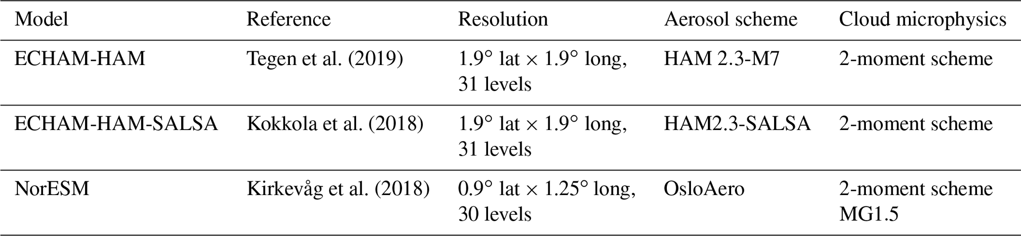
Simulations were performed at T63 (1.9^∘ × 1.9^∘) spatial resolution using 31 vertical levels (L31) and COSP v1.4. Horizontal winds and surface pressure were nudged towards the ERA-Interim (Dee et al., 2011) reanalysis for 2008, and observed sea surface temperatures and sea ice cover for 2008 were used (Taylor et al., 2000). A three-hourly instantaneous output was used. The output of the COSP satellite simulator is also three hourly. The implementation of the COSP satellite simulator in ECHAM-HAM does not allow for instantaneous output. The COSP satellite simulator is called every radiation time step (i.e. every 2 h) and the output of the COSP satellite simulator is averaged over the 3 h output period. This means that on average 50 % of the values in the output of the COSP satellite simulator are instantaneous values (i.e. from only one time step) and 50 % of the values are an average over two radiation time steps (i.e. an average over two instantaneous values which are 2 h apart). The model's properties are summarized in Table 2.

2.3.2 ECHAM-HAM-SALSA

ECHAM-HAM-SALSA is identical to the ECHAM-HAM setup (echam6.3-ham2.3-moz1.0), with the difference being that the sectional aerosol module SALSA (Kokkola et al., 2008, 2018) is used instead of the modal model M7 used in the ECHAM-HAM setup. SALSA calculates the aerosol microphysical processes: nucleation, coagulation, condensation, and hydration. In this setup, the aerosol model HAM also applies the sectional scheme for the rest of the aerosol processes, i.e. emissions, removal, aerosol radiative properties, and aerosol–cloud interactions. In addition to differences in the aerosol size distribution scheme, the wet deposition schemes also differ between the ECHAM-HAM and ECHAM-HAM-SALSA setups. In addition, while ECHAM-HAM uses the cloud activation parameterisation for modal models (Abdul-Razzak and Ghan, 2000), SALSA uses the activation parameterisation for the sectional representation (Abdul-Razzak and Ghan, 2002). Along with the details of these differences, the implementation and the evaluation of SALSA with the ECHAM-HAMMOZ model version, which is used in this study, has been presented by Kokkola et al. (2018).

Similarly to ECHAM-HAM, simulations were performed at T63 (1.9^∘ × 1.9^∘) spatial resolution using 47 vertical levels (L47) and COSP v1.4. Horizontal winds and surface pressure were nudged towards the ERA-Interim (Dee et al., 2011) reanalysis for 2008, and observed sea surface temperatures and sea ice cover for 2008 were used (http://www-pcmdi.llnl.gov/projects/amip/, last access: 14 January 2020). A three-hourly instantaneous output was used. The model's properties are summarized in Table 2.

2.3.3 NorESM

The Norwegian Earth System Model (NorESM) (Kirkevåg et al., 2013; Bentsen et al., 2013; Iversen et al., 2013) is largely based on the Community Earth System Model (CESM) (http://www.cesm.ucar.edu, last access: 17 January 2020) but uses a different ocean model and a different aerosol scheme in the Community Atmosphere Model (CAM) (Collins et al., 2004).

The aerosol microphysics scheme in the NorESM version of CAM, called CAM-Oslo, consists of 12 log-normally shaped background modes which are tagged according to emission source and chemical composition (Kirkevåg et al., 2018). The shape of these modes can change due to condensation and coagulation.

In the current simulations, the NorESM model was run with the CAM-Oslo version 5.3 (Kirkevåg et al., 2018), which is configured with the microphysical two-moment scheme MG1.5 (Morrison and Gettelman, 2008; Gettelman et al., 2015) for stratiform clouds. The scheme includes prognostic equations for liquid (mass and number) and ice (mass and number) and a version of the Khairoutdinov and Kogan (2000) autoconversion scheme where subgrid variability of cloud water (Morrison and Gettelman, 2008) has been included. The aerosol activation into cloud droplets is based on Abdul-Razzak and Ghan (2000) and the heterogeneous freezing in CAM5.3-Oslo is based on Wang et al. (2014) with a correction applied to the contact angle model (Kirkevåg et al., 2018). Moreover, CAM5.3-Oslo has a shallow convection scheme (Park and Bretherton, 2009) and a deep convection scheme (Zhang and McFarlane, 1995). The simulation was run with the Community Land Model (CLM) version 4.5 (Oleson et al., 2010) with satellite phenology. Included in CLM is the Model of Emissions of Gases and Aerosols from Nature (MEGAN) version 2.1 (Guenther et al., 2012), which interactively calculates the emissions of biogenic volatile organic vapours. Both isoprene and monoterpenes take part in the formation of secondary organic aerosol in CAM5.3-Oslo. The sea surface temperatures and sea ice in the simulation were prescribed monthly averages for the years 1982–2001.

The resolution for the simulation was 0.9^∘ × 1.25^∘ and the surface pressures as well as horizontal winds were nudged against ERA-Interim reanalysis data (Berrisford et al., 2011) from 2008. CAM-Oslo was run with COSP version 1.4 producing three-hourly instantaneous outputs. The model's properties are summarized in Table 2.

3 Methods

3.1 Post-processing of the datasets

The comparison of satellite retrievals and model variables is not always straightforward. Satellite-retrieved physical quantities may be derived slightly differently than the corresponding parameters in the model, and differences can be attributed to discrepancies in the retrieved quantities viewed from space versus model fields (i.e. retrieval assumptions, sensor limitations, spatial resolution) (Bodas-Salcedo et al., 2011). In this study we aim at highlighting the differences between observations and models, which stem from different aerosol and cloud physical parameterisation by using the COSP satellite simulator. Satellite simulators, such as COSP, represent a compromise between model fields and retrieved fields. Simulators use model fields to reproduce what the satellite sensor would see if the atmosphere had the clouds of a climate model. By taking the characteristics of the MODIS instrument into account, COSP generates simulated fields of cloud parameters, which can be quantitatively compared to MODIS observations. The COSP diagnostics are then successively aggregated to the simulator outputs and are provided at the original model resolution. Prior to their intercomparison, post-processing of the COSP diagnostics and satellite data is necessary for obtaining a robust evaluation. COSP-derived parameters are in the original model resolution and represent grid-averaged values. As MODIS observations are grid values representative only of in-cloud pixels, the COSP grid-averaged values are divided by the corresponding cloud fractions. The three-hourly outputs from the models were aggregated to daily averages and successively regridded and co-located by linear interpolation onto the finer satellite regular grid of 1^∘ × 1^∘. Each grid point of cloud variables from MODIS observations and MODIS diagnostics was screened using a minimum threshold of 30 % of cloud fraction to minimise the source of errors introduced by the retrieval algorithm and to ensure the existence of large-scale clouds. The screening does not introduce a significant loss in the data pool, or provide grounds for a robust intercomparison as also shown in Bennartz (2007) and Ban-Weiss et al. (2014). For each time step, only grid points having a valid observation simultaneously in each one of the four datasets were included in the final dataset for the statistical analysis.

The MODIS algorithm retrieves cloud properties in the proximity of the top of a cloud, while the direct model outputs provide values through the entire vertical structure of a simulated atmospheric column. To overcome this issue, when comparing the direct model output CDNC and satellite-derived CDNC, we selected the column maximum value of the CDNC direct output of the models for each grid box. Additionally, we selected only grid points with temperature T>273 K to exclude mixed-phase and ice clouds.

Note that all discussed cloud parameter are diagnosed using satellite simulators and are compared to the corresponding MODIS satellite observations. However, we use two direct model diagnostics in the study:

• AOD, which is used to derive the AI, a proxy for cloud condensation nuclei for the computation of ACI,

• CDNC_direct, which is compared with COSP-simulated and MODIS-derived estimates.

3.2 Cloud droplet number concentration (CDNC)

The CDNC values were derived from CER and COT from MODIS observations and COSP simulations by combining Eqs. (6) and (9) from Bennartz and Rausch (2017) in the following equation:

$$\begin{array}{}\text{(1)}& \mathrm{CDNC}=\mathit{\gamma }\cdot {\mathrm{COT}}^{\mathrm{0.5}}\cdot {\mathrm{CER}}^{-\mathrm{2.5}},\end{array}$$

where COT is cloud optical thickness, CER is the cloud droplet effective radius, and $\mathit{\gamma }=\mathrm{1.37}\times {\mathrm{10}}^{-\mathrm{5}}$ m^0.5 (Quaas et al., 2006). The assumption of not accounting for the temperature effect and setting γ as a bulk constant applies rather well to the warm stratiform clouds in the marine boundary layer but less so for convective clouds (Bennartz, 2007; Rausch et al., 2010; Grosvenor et al., 2018). The equation represents the “Idealized Stratiform Boundary Layer Cloud” (ISBLC) model (Bennartz and Rausch, 2017), which is based on the following assumptions:

• the cloud is horizontally homogeneous;

• the LWP increases linearly from the cloud base to the cloud top;

• the CDNC is constant throughout the vertical extent of the cloud.

While the ISBLC model describes important aspects of stratiform boundary layer clouds, its assumption will never be fully valid for a real cloud. Issues related to the ISBLC model assumptions are extensively elaborated in Bennartz (2007) and Bennartz and Rausch (2017) and references therein. Despite the above-mentioned approach for deriving CDNC over land ares, we will provide MODIS CDNC values globally (land and ocean). These estimates will be used as a reference dataset, rather than “truth” data, for enabling the comparison of COSP-derived CDNC and the model direct output of CDNC.

3.3 Assessing the aerosol–cloud interactions

The aerosol–cloud interactions are quantified here trough the parameter ACI_CDNC defined as the change in the selected cloud property, CDNC, to a change in AI, which is used here as a proxy for cloud condensation nuclei (CCN):

$$\begin{array}{}\text{(2)}& {\mathrm{ACI}}_{\mathrm{CDNC}}={\displaystyle \frac{\mathrm{d}\ln \left(\mathrm{CDNC}\right)}{\mathrm{d}\ln \left(\mathrm{AI}\right)}}.\end{array}$$

The CDNC was computed from the CER and COT from the COSP-MODIS simulations and MODIS retrievals. Additionally, AI was derived from ECHAM-HAM, ECHAM-HAM-SALSA, and NorESM MODIS-COSP diagnostics, and MODIS satellite observations following Feingold et al. (2001). The mean values and standard deviations of the parameters involved in the computation of ACI_CDNC are presented in Table 1. We discarded pixels retrieved when liquid cloud fraction is ≤0.3 to reduce noise contamination and to focus on large-scale clouds. The screened parameters were used to derive CDNC. The ACI_CDNC parameter was calculated globally for each season. When calculating the ACI_CDNC for the 1^∘ × 1^∘ grid boxes, Eq. (2) is applied to data for the selected season and grid box. This methodology (Grandey and Stier, 2010) can be thought of as computing the linear regression slope of a scatter plot of ln(CDNC) versus ln(AI), where each point represents a day for which both aerosol and cloud data exist for the considered grid box. When computing ACI_CDNC for large areas, the ACI_CDNC of each grid box needs to be weighted by the corresponding number of data points (Grandey and Stier, 2010). This step was included in the post-processing of the datasets.

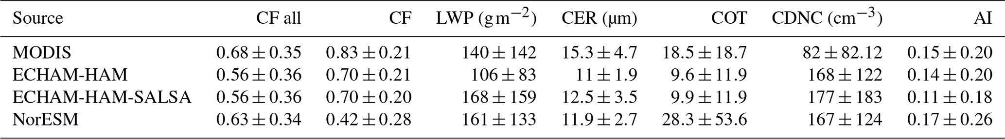
Table 1 Annual global in-cloud mean value ± standard deviation for the parameters used in the study. If a grid point has CF ≤30 %, the point is set to fill values in all the datasets. The process leads to a 35 % reduction in data points in each dataset. “CF all” is not screened for CF ≤30 %. AI values are representative of ocean values only.

Tegen et al. (2019)Kokkola et al. (2018)Kirkevåg et al. (2018)

Table 2 Summary of the models used in the study.

4 Results

4.1 Global bias distributions

In this section we compare on a global scale aerosol and cloud properties from the three models by subtracting MODIS retrievals from the modelled COSP diagnostics. From now on we will refer to the difference between the simulated parameters and MODIS retrieved values using the term bias.

Overall, the spatial distributions of the biases (Figs. 1–5) show large discrepancies around the polar and ice-covered areas, such as Greenland and Antarctica. Over these areas large discrepancies are expected due to the inaccuracy of the MODIS retrieval algorithm due to viewing geometry (i.e. large zenith or viewing angles) and to correctly classify opaque clouds, snow/ice surfaces, and optically thin clouds over really bright or warm surfaces (Marchant et al., 2016).

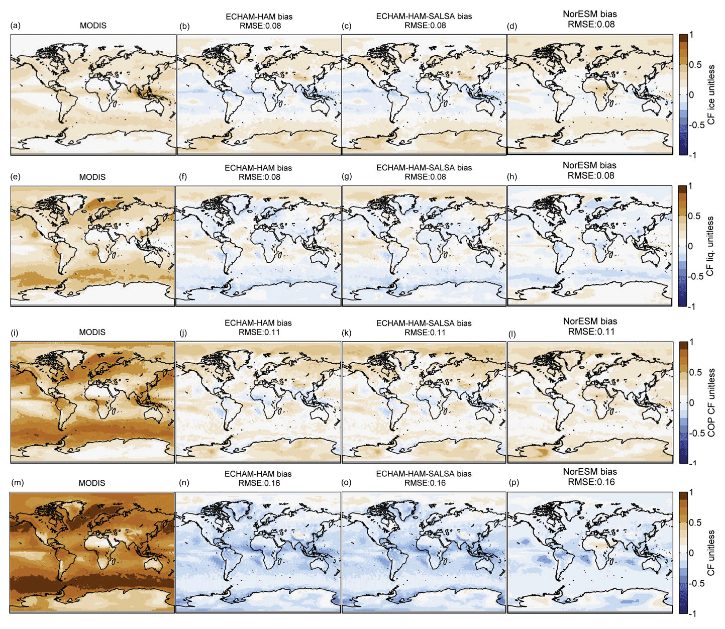
Figure 1 Annual global mean bias in cloud fraction. The bias represents the difference between MODIS-COSP diagnostics from ECHAM-HAM, ECHAM-HAM-SALSA, NorESM, and MODIS observations. COSP-simulated total ice and liquid cloud fractions are compared with MODIS retrieval ice fraction (b–d) and with MODIS retrieval liquid cloud fraction (f–h), respectively. COSP-simulated total cloud fraction is compared with MODIS retrieval total cloud fraction (COP CF) (j–l) and cloud mask cloud fraction (CF) (n–p). Pixels with liquid cloud fraction ≤30 % are screened.The averages represent in‐cloud values. High latitudes (lat >60^∘ N or lat >60^∘ S) are excluded in the computation of the root mean square error (RMSE). MODIS spatial distribution is presented as reference (a, e, i, m).

Figure 1 presents the differences between the MODIS-COSP cloud fraction diagnostics and COP CF for ice clouds CF_ice (Fig. 1b–d), and liquid clouds CF_liq (Fig. 1f–h), as well as the differences between MODIS total COP CF (Fig. 1j–l), and CF (Fig. 1n–p). Additionally, for each comparison the MODIS spatial distribution is presented as reference (Fig. 1a, e, i, m). It was already highlighted in Sect. 2.1 that the cloud fraction retrieved from the optical properties (CF_ice, CF_liq, and COP CF) excludes partly cloudy pixels, representing a limitation in the comparison of the data. Thus, lower values of MODIS COP cloud fractions are expected. A widespread positive bias is observed for CF_ice and CF_liq, indicating higher values of the COSP-simulated cloud fractions than the MODIS observations. Prevalent cloud regimes can be recognised in the bias distributions. ECHAM-HAM and ECHAM-HAM-SALSA represent the amount of ice clouds well, which are generally found in the Intertropical Convergence Zone (ITCZ) and the marine subtropical stratocumulus and stratus regions, whereas liquid clouds are better represented over land areas and in the subtropical stratocumulus region. NorESM shows positive biases for ice cloud amount over stratus cloud regions and around the ITCZ, but it shows smaller biases for liquid stratus cloud regimes than ECHAM-HAM and ECHAM-HAM-SALSA.

The total cloud fraction bias shows a positive bias between the MODIS-COSP CF simulated by the three models and MODIS COP CF (Fig. 1j–l) and a negative bias when MODIS CF is considered (Fig. 1n–p). Consequently, MODIS CF is higher than the MODIS COP CF product. This outcome is to be expected, and it possibly originates from the different treatment in the MODIS algorithm of partly cloudy pixels in the computation of CF and COP CF, as discussed in Sect. 2.1. Additionally, all models underestimate CF in marine subtropical stratocumulus regions.

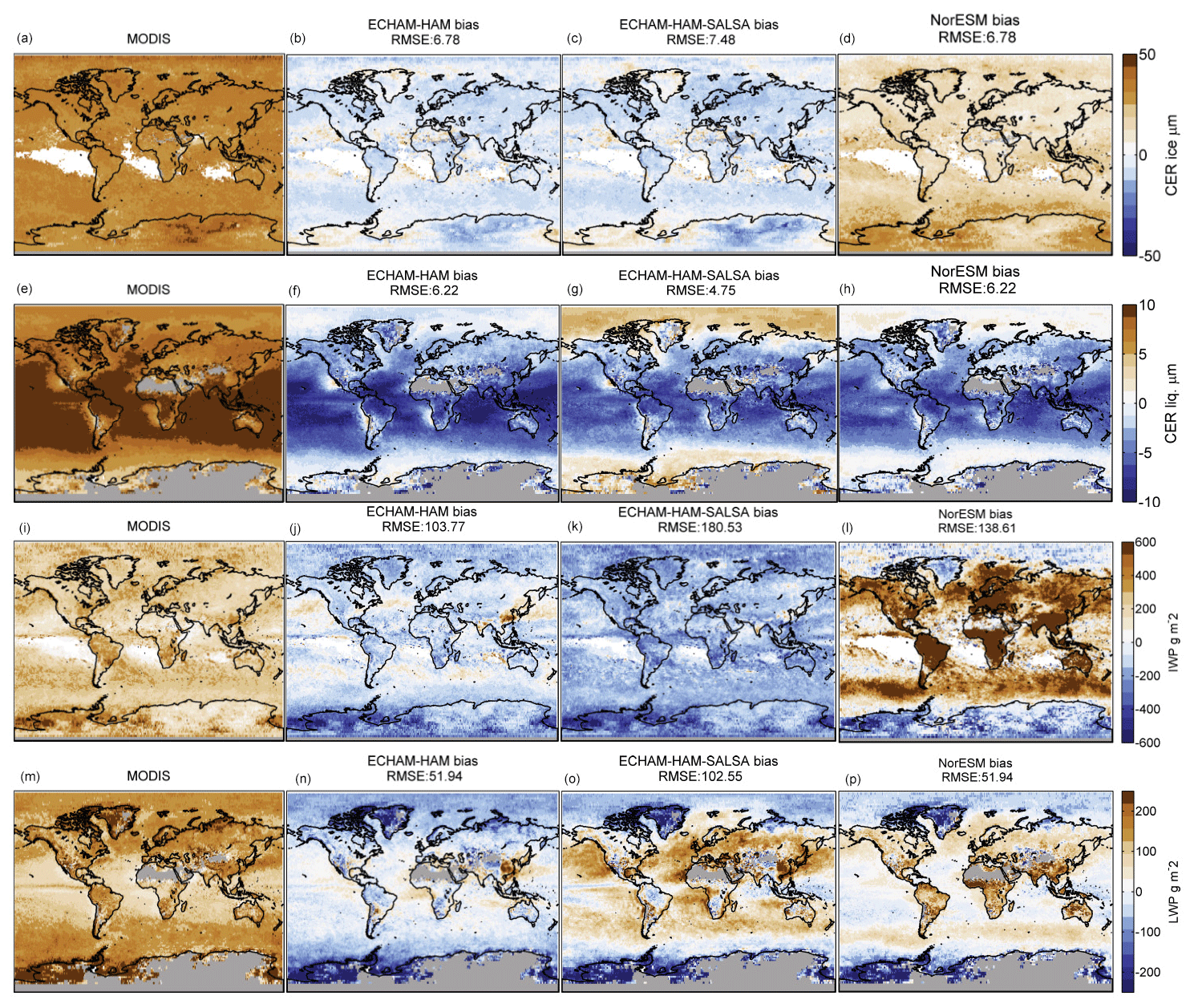
Figure 2 Annual global mean bias in cloud effective radius and water path. The bias represents the difference calculated by subtracting MODIS observation to MODIS-COSP diagnostics from ECHAM-HAM, ECHAM-HAM-SALSA, and NorESM. Ice cloud effective radius (CER_ice) from MODIS-COSP is compared with MODIS observations in (b)–(d) and liquid cloud effective radius (CER_liq) in (f)–(h). The biases related to the comparison of COSP-simulated ice water path (IWP) are showed in (j)–(l) and for liquid water path (LWP) in (n)–(p). Pixels with liquid cloud fraction ≤30 % are screened. The averages represent in‐cloud values. Pixels with liquid cloud fraction ≤30 % are screened. Values are in‐cloud concentrations. High latitudes (lat >60^∘ N or lat >60^∘ S) are excluded in the computation of the root mean square error (RMSE). MODIS spatial distribution is presented as reference (a, e, i, m).

The spatial distribution of the cloud physical and optical properties is remarkably similar among the model datasets with the exception of CER_ice, IWP (Fig. 2d and l), and COT (Fig. 3g, k) for NorESM. These strong biases are explained by the fact that in the NorESM COSP 1.4 implementation code includes radiative active snow in the computation of the effective radius and optical thickness of ice clouds. However, this does not affect the properties of liquid clouds.

CER_ice and IWP are underestimated in ECHAM-HAM and ECHAM-HAM-SALSA. This is likely caused by the cirrus scheme which does not account for heterogenous nucleation or pre-existing ice crystals during formation of cirrus clouds (Neubauer et al., 2019; Lohmann and Neubauer, 2018). Interestingly, dissimilarities can also be observed between ECHAM-HAM and ECHAM-HAM-SALSA, despite the fact that the models share the same cloud module. ECHAM-HAM CER_liq is on average 5 µm smaller than in ECHAM-HAM-SALSA in the mid-latitude belt, and ECHAM-HAM-SALSA CER_liq is larger around the polar areas (Fig. 2g) and shows a large positive bias for LWP over ocean (Fig. 2o) in comparison to ECHAM-HAM. LWP is also overestimated by NorESM but only over land areas (Fig. 2p), while ECHAM-HAM shows a good agreement with MODIS (Fig. 2n).

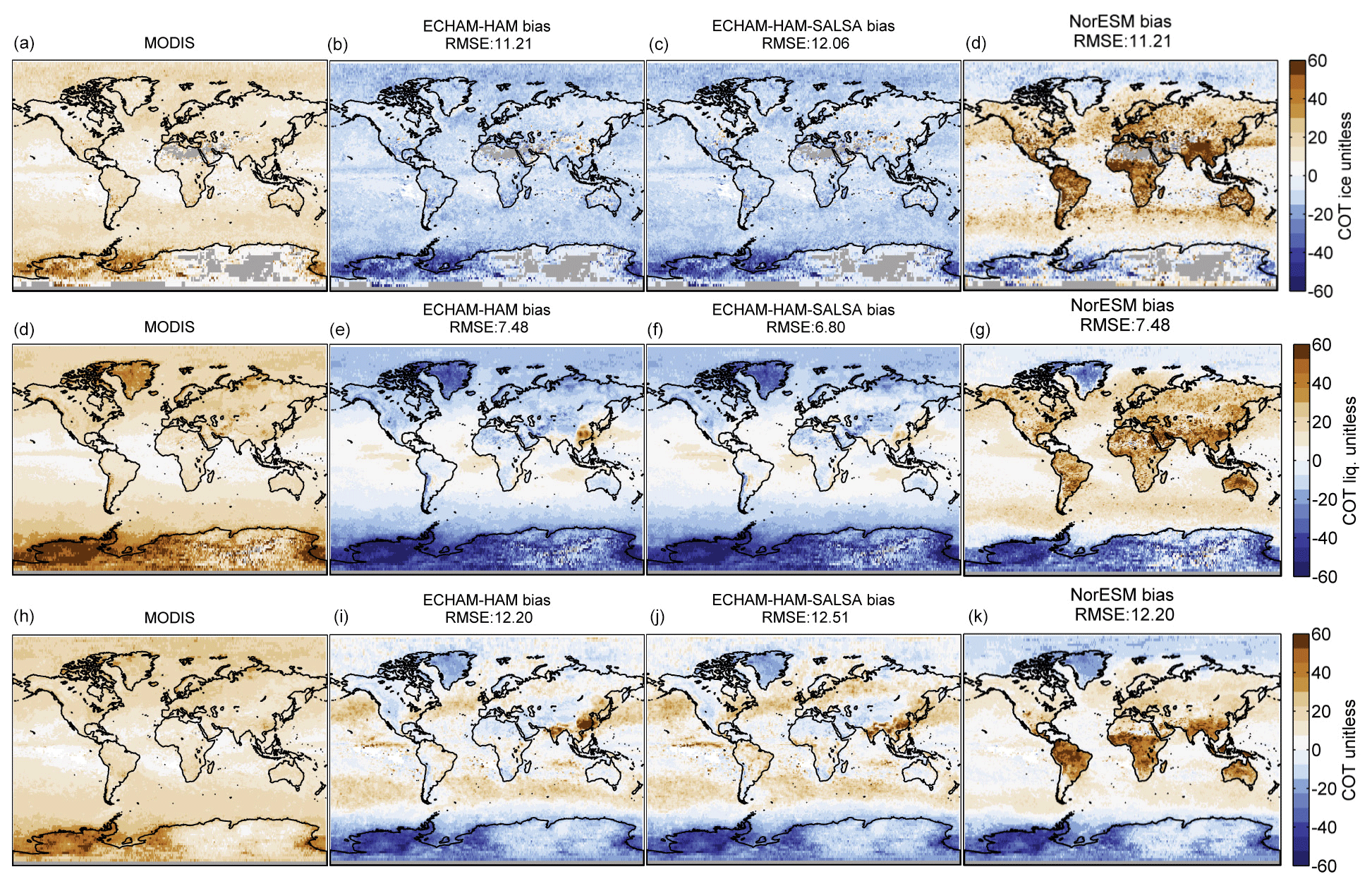
Figure 3 Annual global mean bias in cloud optical thickness for ice clouds (b–d), liquid water clouds (e–g), and total (combined ice and water clouds) COT (i–k) between MODIS and ECHAM-HAM, ECHAM-HAM-SALSA, and NorESM. The bias represents the difference between MODIS-COSP diagnostics and MODIS observations. Pixels with liquid cloud fraction ≤30 % are screened. The averages represent in‐cloud values. High latitudes (lat >60^∘ N or lat >60^∘ S) are excluded in the computation of the root mean square error (RMSE). MODIS spatial distribution is presented as reference (a, d, h).

The evaluation of COT shows homogeneous results and comparable values of root mean square errors (Fig. 3) with the exception of NorESM COT biases for ice and liquid clouds, which are particularly high over land. It appears that some tuning parameters, for example the autoconversion parameter, are particularly low and affect the convection scheme by suppressing precipitation, thus creating thick clouds. The comparison of the differences between the biases of ECHAM-HAM and of ECHAM-HAM-SALSA shows localised differences over India, China, and Russia for IWP (Fig. 2j, k) and over China for water cloud COT (Fig. 3e, f). These are also regions where aerosol microphysics has a fundamental role as shown in Kokkola et al. (2018). ECHAM-HAM and ECHAM-HAM-SALSA generally overestimate COT. The atmospheric model ECHAM shows a similar estimation when running without an aerosol model. This overestimation has been previously reported by Stevens et al. (2013).

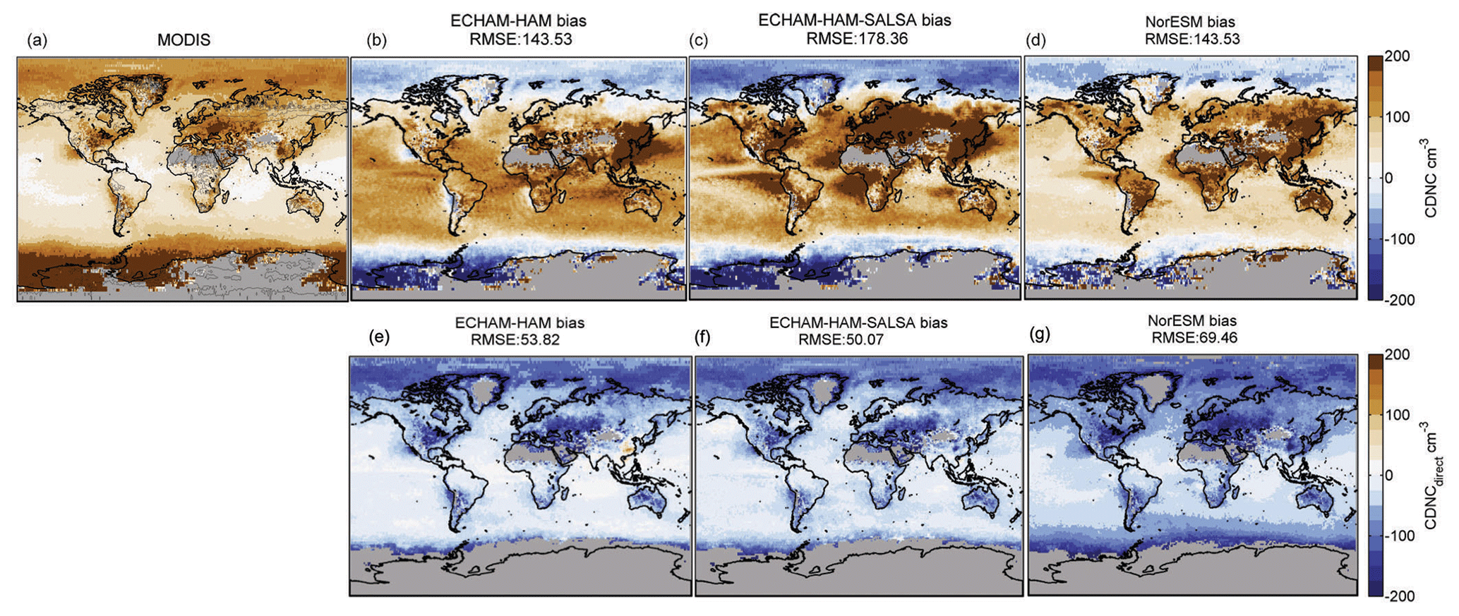
Figure 4 Cloud droplet number concentration (CDNC) annual mean bias. The bias represents the difference between CDNC derived from MODIS-COSP diagnostics and MODIS observations (b–d) and the model direct outputs and MODIS observations (f–h). Pixels with liquid cloud fraction ≤30 % are screened. The averages represent in‐cloud values. High latitudes (lat >60^∘ N or lat >60^∘ S) are excluded in the computation of the root mean square error (RMSE). MODIS spatial distribution is presented as reference (a). Contour lines highlight the land areas where the assumptions for deriving MODIS CDNC are less reliable.

Figure 4 shows global biases for CDNC values derived from the MODIS retrievals and the COSP diagnostics following the method presented in Sect. 3.2 (Fig. 4b–d) and the daily averages of the direct output of the models (Fig. 4e–g). The CDNC derived from MODIS (Fig. 4a) are shown globally (land and ocean) despite the fact that assumptions described in Eq. (1) are less reliable over land areas, which are highlighted with contour lines. The differences between MODIS-COSP diagnostics and MODIS observations are very clear. Overall the MODIS-derived CDNC values are lower than these derived from COSP simulated values but higher than the direct output values. Consequently, the CDNC from direct model output is lower than MODIS-COSP diagnostics. Possible explanations could be either related to the COSP method for deriving CER_liq and COT_liq or the approach used for deriving CDNC from CER_liq and COT_liq, or they could be related to the fact that the computation of the direct CDNC requires a minimum CDNC set to 40 cm⁻³. This outcome is very similar to what has been found by Ban-Weiss et al. (2014), where the CDNC satellite-simulated values are higher than the standard CAM5 model output near cloud top as well as the column maximum values. Therefore, this result represents an interesting topic that extends beyond the scope of this paper, but it should be further developed in future work. The biases between CDNC-COSP-derived and modelled direct values are very different, but within each product the biases are similar, although local differences are observed. For example, the CDNC values from ECHAM-HAM-SALSA are lower in the polar regions and higher in the mid-latitude belt in comparison with the ECHAM-HAM and NorESM diagnostics. Local differences can also be observed in the direct output where ECHAM-HAM-SALSA shows higher values of CDNC over the oceans in the Southern Hemisphere (Fig. 4f). A direct comparison of CDNC derived from MODIS-COSP-simulated variables and the model CDNC direct outputs is shown in the Supplement. ECHAM-HAM and ECHAM-HAM-SALSA were run with identical tuning parameter settings which were optimised for ECHAM-HAM. This choice was made to distinguish the differences in aerosol–cloud interactions coming from different aerosol microphysics modules. The differences in CDNC between these two model setups originate from the cloud activation schemes, i.e. for HAM the modal cloud activation scheme of Abdul-Razzak and Ghan (2000) and for HAM-SALSA the sectional cloud activation scheme (Abdul-Razzak and Ghan, 2002). The cloud activation scheme of ECHAM-HAM-SALSA produces a higher CDNC than ECHAM-HAM (Fig. 4c), because the SALSA microphysics module simulates generally a higher number of particles larger than 100 nm in diameter, which act as cloud condensation nuclei. Despite the higher CDNC, CER_liq is larger in ECHAM-HAM-SALSA than in ECHAM-HAM. Although it is expected that CER_liq decreases with increasing CDNC, higher LWP in ECHAM-HAM-SALSA in turn results in larger CER_liq and outweighs the CDNC effect on CER_liq. The causes for differences in LWP between the two model versions are very difficult to diagnose but candidates for causing them are differences in wet scavenging, convective detrainment, or freezing.

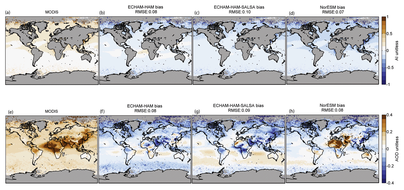
Figure 5 Aerosol index (AI) (b–d) and aerosol optical depth (f–h) annual mean bias. AI values are representative of ocean values only. The bias represents the difference between the model direct outputs and MODIS observations. High latitudes (lat >60^∘ N or lat >60^∘ S) are excluded in the computation of the root mean square error (RMSE). MODIS spatial distribution is presented as reference (a, e).

Figure 5 presents AOD and AI biases. The biases between values of AI from direct model output and MODIS observations are quite close among the models as their average is about of +0.2. The main divergence is observed in the ECHAM-HAM bias where higher AI values are simulated around the mid-latitude belt. Tegen et al. (2019) found indications that the particle size of mineral dust and sea salt aerosol particles may be too small in ECHAM-HAM. More discrepancies can be observed in the AOD bias: ECHAM-HAM-SALSA AOD values are higher over ocean, and NorESM AOD values are much higher over deserts and other bright surfaces (such as Africa and Australia). Other localised distinctions in aerosol loading distribution can be observed over regions which are typically strongly affected by primary emissions (such as the Sahara, India, Southeast Asia, Russia, Canada, central Africa, and South America). The different representations of size distribution, microphysical processing of aerosols, and sink processes have a significant effect on the modelled AOD, as shown for the aerosol module SALSA2.0 by Kokkola et al. (2018). The overestimation of AOD in the tropical oceans and underestimation of AOD at higher latitudes and over land in ECHAM-HAM has also been found by Tegen et al. (2019).

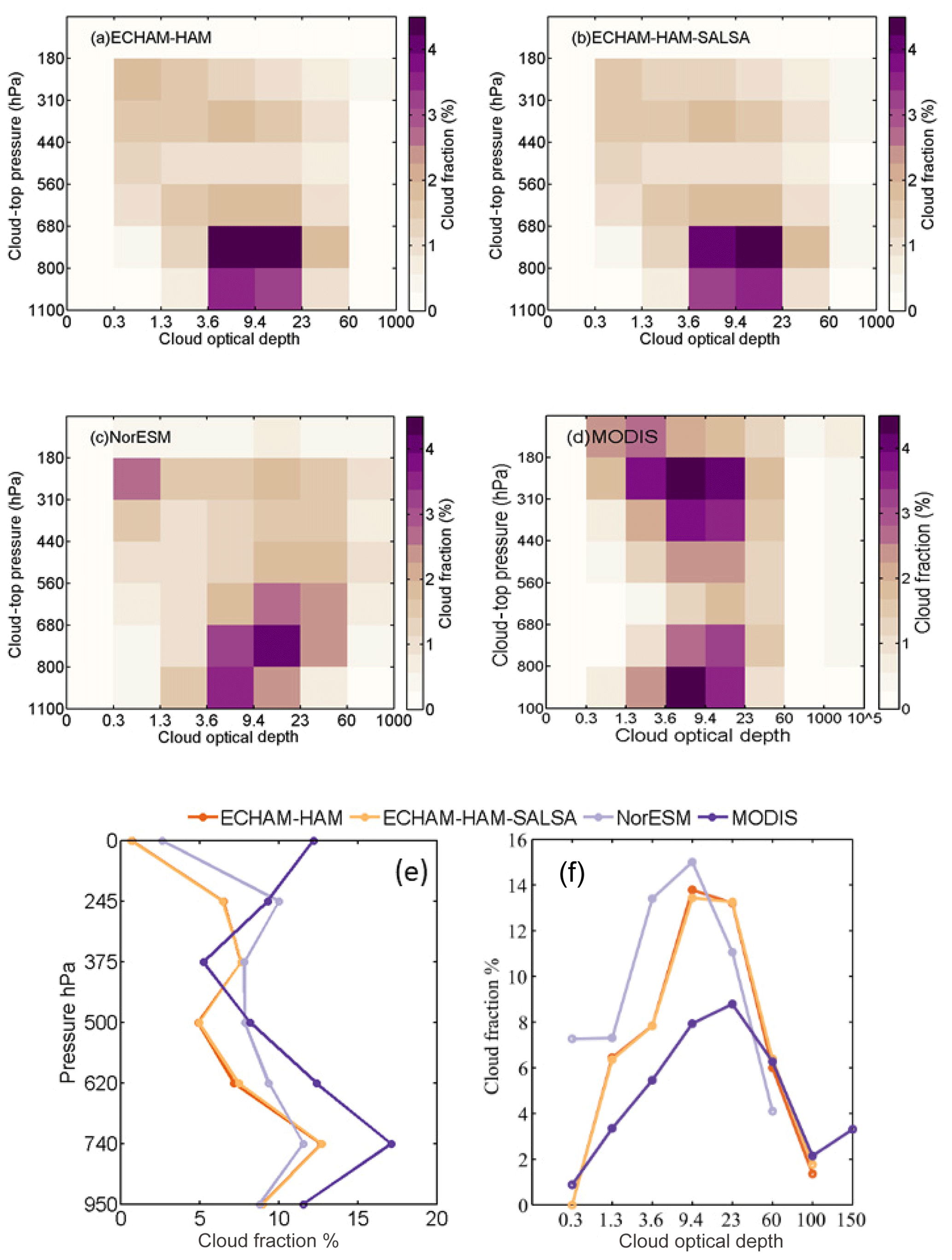
Figure 6 Vertical distribution analysis. Cloud fraction as a function of cloud-top pressure (CTP) and optical thickness for (a) ECHAM-HAM, (b) ECHAM-HAM-SALSA, (c) NorESM, and (d) MODIS. The colour scale represents the cloud fraction percentage. (e) Cloud fraction as a function of CTP (sum of all optical depth ≥0.3), and (f) cloud fraction as a function of COT (sum of all CTP layers for each COD-bin).

4.2 Joint histogram

The analysis of the CTP-COT joint histogram enables us to determine how well the data sources represent the vertical cloud structures and regimes. Figure 6 shows the comparison of the simulated and observed global mean cloud fraction as a function of cloud-top pressure (CTP) and cloud optical thickness. ECHAM-HAM and ECHAM-HAM-SALSA (Fig. 6a, b) show a nearly identical result by concentrating a large fraction of clouds at low level (CTP≤680 hPa) and in the interval $\mathrm{3.6}\le \text{COT}\le \mathrm{23}$. NorESM (Fig. 6c) also concentrates its largest amount of clouds at low levels in the same COT interval as in Fig. 6a and b, but it detects also a higher fraction (about 2 %–2.5 %) of optically thick clouds, $\mathrm{9.4}\le \text{COT}\le \mathrm{60}$, throughout the atmosphere. A second cloud fraction peak is observed for optically thin clouds (COT≤1.3) at very high levels ($\mathrm{180}\le \text{CTP}\le \mathrm{310}$) for NorESM. This bimodal distribution resembles the vertical distribution of the MODIS cloud fraction shown in Fig. 6d. The MODIS observations are mostly in the category of high-level clouds (CTP≤440 hPa) and low-level clouds (680 hPa≤CTP). MODIS shows on average more mid-level clouds than NorESM and a higher fraction at low level for $\mathrm{3.6}\le \text{COT}\le \mathrm{23}$ similarly to ECHAM-HAM and ECHAM-HAM-SALSA. Figure 6e shows the differences in cloud vertical distribution where MODIS is generally having the highest cloud fraction except for mid-level clouds. MODIS also presents the highest percentage of clouds for COT≥3.6. NorESM and MODIS detect nearly the same amount of clouds for $\mathrm{1.3}\le \text{COT}\le \mathrm{3.6}$, while for optically very thin clouds (COT≤1.3) a good agreement is obtained between all datasets, and NorESM shows the highest percentage of cloud fractions.

4.3 Aerosol–cloud interactions

The daily mean values of CDNC and AI were used to assess how clouds are affected by the changes in the CCN proxy. Uncertainties were computed as the 95 % confidence intervals using daily averages. Positive estimates of ACI_CDNC indicate an increase in CDNC as a function of AI, which could be an indication of the aerosol indirect effects. The potential limitations to this approach are discussed in Sect. 5.

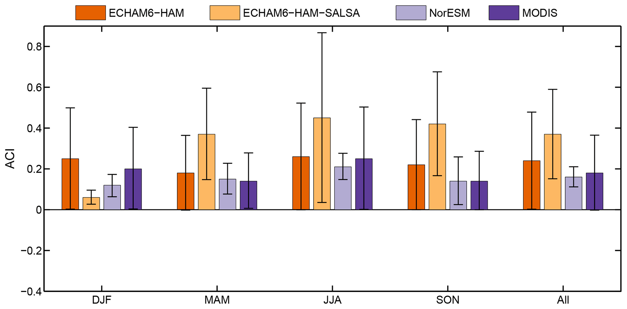
Figure 7 Global (over ocean only) estimates of the ACI_CDNC computed as the changes in ln(CDNC) to ln(AI). CDNC values are derived from corresponding daily grid points of LWP and COT from MODIS observations and COSP-MODIS outputs following Bennartz (2007). ACI_CDNC values are calculated by season and for the entire period (1 January 2008–31 December 2008). Uncertainty estimates are calculated as 95 % confidence interval from the daily values.

Figure 7 shows estimates of ACI_CDNC on a global scale, although over ocean areas only, for each season and, separately, for the entire period under study as “All”. The same analysis is iterated on a regional scale, including both land and ocean areas, and presented in the Supplement (Fig. S4) Error bars are representative of the boundaries of the 95 % confidence interval. The positive ACI_CDNC values resulting from MODIS and the three models suggest that changes in AI are connected with an increase in CDNC and the trend seems to be independent of the time of the year. The modelling ACI_CDNC estimates are similar in the models; however, the results are statistically indistinguishable owing to fully overlapping confidence bars (Cumming et al., 2007). MODIS ACI_CDNC estimates show negative values for the winter months (DJF), especially over the Northern Hemisphere (Fig. S4). As these negative values are derived over land regions, it could be indicative of retrieval biases over bright surfaces (i.e. snow or ice). Furthermore, it is important to inform the readers that MODIS aerosol size parameters over land (i.e. AE or fine-AOD) are no longer official products directly provided by the MODIS aerosol team. The publication of these variables was discontinued due to low quantitative MODIS skill (Mielonen et al., 2011; Levy et al., 2013). Using spectral AOD, we derived AE over land and derived AI on a global scale to allow for estimates of ACI_CDNC on a global scale (Fig. S4). However, the AE values over land were not evaluated. However, negative ACI_CDNC values may be associated with the presence of different types of aerosol (i.e. hydrophobic aerosol such as dust, black carbon) and their proximity to clouds, which may affect or inhibits the growth of cloud droplets (Chen et al., 2018; Jiang et al., 2018; Costantino and Bréon, 2013). Over ocean negative ACI_CDNC values from MODIS observations have been systematically found over subtropical marine stratocumulus regions (i.e. N. Atlantic Ocean, N. America, S. Atlantic Ocean). In these regions Chen et al. (2014) found a decrease in LWP with increasing AI for non-precipitating scenes. Additionally, negative ACI_CDNC values were suggested owing to wet scavenging or mixing of environmental air by entrainment (Ackerman et al., 2004). While both processes affect LWP, CDNC is not necessarily changing. This indicates limits in the derivation of CDNC from retrieved quantities for MODIS. Also water uptake by aerosol particles and effects of meteorology can have a significant impact on the estimation of ACI_CDNC derived from the relationship between CDNC and AI (Neubauer et al., 2017).

Cloud properties (Figs. 2 and 3) are more similar for ECHAM-HAM and ECHAM-HAM-SALSA, which share the same atmospheric model, rather than between the two models and NorESM. Nevertheless, the ACI_CDNC estimates show good agreement between the three models and, even more important, with ACI_CDNC derived from MODIS observations.

5 Summary, discussion, and conclusions

The differences between observed and modelled aerosol and cloud properties can be related to many factors, among which are the different parameterisations of aerosol and cloud physical processes in the models or differences in observation characteristics by satellite, as well as meteorological influences on aerosol–cloud interactions. In this study we focus on the differences due to the physical parameterisation of aerosol and cloud properties, and we minimise the impact of the other factors. This objective was achieved by using a satellite simulator, which resolves the issue related to the incongruities between model and satellite views, and by nudging modelled winds to meteorological observation, solving the discrepancies between observed and modelled meteorology.

The results show that the aerosol module in a climate model, in our case ECHAM-HAM and ECHAM-HAM-SALSA, has a smaller effect on the simulation of cloud properties than switching to another atmospheric model, such as NorESM. However, the three models differ from each other in the spatial and vertical representation of clouds. The COSP cloud fraction diagnostics are comparable to MODIS products but the difference between the two MODIS products of total cloud fractions is significant. Despite having identical cloud modules, ECHAM-HAM and ECHAM-HAM-SALSA diverge when comparing liquid water cloud properties, yet both fail to represent high level clouds. The discrepancies between ECHAM-HAM and ECHAM-HAM-SALSA may originate from different amounts of activated droplets and different ice nucleation rates. While the NorESM cloud vertical distribution is closer to MODIS, large biases are found globally for cloud droplet size and water content in ice clouds due to the contribution of radiatively active snow (Kay et al., 2012). The inclusion of radiatively active snow in the physical model and the COSP module mitigates the underestimation of model mid-level clouds and high clouds, but it heavily impacts the magnitude of the global values of the cloud properties in ice clouds.

The differences observed in the simulation of cloud properties are reflected in the estimations of ACI_CDNC. ACI_CDNC is generally larger for ECHAM-HAM-SALSA, while similarly lower values are found for ECHAM-HAM, NorESM, and MODIS.

Although satellite simulators allow for robust comparisons, their reliability is flawed when the observational data are not well explained or the simulator itself fails to address specific characteristics. Therefore, their strengths and weaknesses need to be accounted for to successfully use simulation diagnostics in model–observation comparisons as illustrated in detail by Pincus et al. (2012) and Kay et al. (2012). For example, simulators have limitations in depicting horizontally heterogeneous cloud regimes as they do not account for sub-pixel clouds, which may explain the differences in the detection of small cloud fractions between observations and models. However, simulator and observational errors are here neglected, because we considered them to be less important in the explanation of the model biases. The observed biases in the modelled clouds could originate from errors in the model calculation as well from the cloud parameterisation; the identification of the specific reasons for these discrepancies is beyond the scope of this study.

The results presented here indicate that the cloud droplet number concentration appears to be more sensitive to changes in aerosols in models than observations, and these results are in agreement with many previous studies found in the literature (e.g. Ban-Weiss et al., 2014; Quaas et al., 2004; McComiskey and Feingold, 2012; Penner et al., 2011). Some of the challenges and limitations in assessing ACI_CDNC are now highlighted. AOD retrievals are limited to cloud-free conditions, which creates challenges for studying the ACI_CDNC, where the intention is to study co-located aerosol and cloud observations. Unless height-resolving instruments (i.e. lidars) are considered, the vertical location of the AOD level is unknown. Aerosol and cloud measurements may contain retrieval errors, which are further propagated to ACI_CDNC estimates, and they reciprocally may bias the respective retrievals (Jia et al., 2019) . The interpretation of the observed aerosol–cloud relationships is complicated by the effect of meteorology (Quaas et al., 2010; Gryspeerdt et al., 2014, 2016; Brenguier et al., 2003). As cloud formation happens in high-humidity conditions, aerosol humidification can severely affect the assessment of ACI by causing positive correlation between AOD and cloud properties (Myhre et al., 2007; Quaas et al., 2010; Grandey et al., 2013; Gryspeerdt et al., 2014). Additionally to aerosol particles, water vapour also affects precipitation (Boucher et al., 2013), obviously linked to the presence of clouds, and consequently causes spurious correlations between aerosols and clouds (Koren et al., 2012). Therefore, some of the differences in the ACI_CDNC estimates from satellites and models could be associated with limitations in satellite measurements. For example, the estimates of ACI_CDNC might suffer from an averaging effect due to the large spatial averages of satellite aerosol and cloud properties. L3 data can introduce spurious relationships between aerosols and cloud properties (e.g. McComiskey and Feingold, 2012; Christensen et al., 2017), and they provide a rather limited pool of data samples enabling the analysis only over large regions. This was not explored in this study because we used the same spatial resolution for both the true model estimate and for the satellite-based model estimate for the ACI_CDNC. Neubauer et al. (2017) performed a detailed study on the impact of meteorology, cloud regimes, aerosol swelling, and wet scavenging on microphysical cloud properties using ECHAM-HAM. The results highlight that a minimum distance between cloud and aerosol gridded data should be taken into account in the analysis of satellite data; they also highlight that dry aerosols should be selected to reduce the influence of aerosol growth due to humidity for model simulations when comparing satellite-based and model estimates for ACI_CDNC. Similarly to our results, Neubauer et al. (2017) find a systematical overestimation of the sensitivity of modelled LWP and CDNC compared to MODIS observations and often a disagreement in sign in the comparison of cloud parameters. The results suggest that the derivation of CDNC from satellite observations may be limited by entrainment mixing of environmental air or precipitation. Furthermore, the models can not resolve the entrainment mixing at the top of stratocumulus clouds, which puts the LWP sensitivity to aerosol change in the models into question. In conclusion, this study identified limitations and deficiencies in the models, and their acknowledgement is important for the model development process and the correct interpretation of modelling diagnostics. We highlighted many discrepancies in cloud spatial and vertical representations and the results showed that the three models overall similarly underestimate cloud fraction for the stratocumulus cloud regime being when compared to MODIS. We discovered that IWP is systematically lower in ECHAM-HAM-SALSA than in ECHAM-HAM due to a higher cloud droplet freezing rate, which consecutively triggers a reduced sedimentation of ice clouds. This outcome explains the contradictory result in ECHAM-HAM-SALSA that shows the largest global averages for CER among the models despite having the highest CDNC. Further investigation is needed to explain the differences in ice cloud properties between ECHAM-HAM and ECHAM-HAM-SALSA. The clouds simulated by NorESM are too thick over land and this issue is not only seen in COSP variables but also in the default model output due to a very low autoconversion parameter, which caused the suppression of precipitation over land, and thus thicker clouds. Additionally, in support to Ban-Weiss et al. (2014), the study revealed that the direct model CDNC is systematically larger than the values derived from COSP diagnostics and MODIS observation. These discrepant results from the comparison of COSP-derived CDNC and the modelled direct output of CDNC, where the MODIS data represent solely the reference dataset rather than “truth” data, stem from the aerosol model setup, and this discrepancy has potentially important implications for the modelling community using satellite observations to evaluate standard (not satellite-simulated) model output.

Finally, we point out that the model deficiencies identified here may lead to an improvement in model parameterisation and to more robust results. As future work, a regional-based analysis would enable a better understanding of the physical processes responsible for the model biases. Additional research should be conducted to evaluate the aerosol–cloud interaction following the approach suggested by Neubauer et al. (2017). These further steps would potentially benefit the modelling community interested in climate applications.