Modeling atmospheric ammonia using agricultural emissions with improved spatial variability and temporal dynamics

Ammonia emissions into the atmosphere have increased substantially in Europe since 1960, primarily due to the intensification of agriculture, as illustrated by enhanced livestock and the use of fertilizers. These associated emissions of reactive nitrogen, particulate matter, and acid deposition have contributed to negative societal impacts on human health and terrestrial ecosystems. Due to the limited availability of reliable measurements, emission inventories are used to assess large-scale ammonia emissions from agriculture by creating gridded annual emission maps and emission time profiles globally and regionally. The modeled emissions are subsequently utilized in chemistry transport models to obtain ammonia concentrations and depositions. However, current emission inventories usually have relatively low spatial resolutions and coarse categorizations that do not distinguish between fertilization on various crops, grazing, animal housing, and manure storage in its spatial allocation. Furthermore, in assessing the seasonal variation of ammonia emissions, they do not consider local climatology and agricultural management, which limits the capability to reproduce observed spatial and seasonal variations in the ammonia concentrations.

This paper describes a novel ammonia emission model that quantifies agricultural emissions with improved spatial details and temporal dynamics in 2010 in Germany and Benelux. The spatial allocation was achieved by embedding the agricultural emission model Integrated Nitrogen Tool across Europe for Greenhouse gases and Ammonia Targeted to Operational Responses (INTEGRATOR) into the air pollution inventory Monitoring Atmospheric Composition and Climate-III (MACC-III), thus accounting for differentiation in ammonia emissions from manure and fertilizer application, grazing, animal houses and manure storage systems. The more detailed temporal distribution came from the integration of TIMELINES, which provided predictions of the timing of key agricultural operations, including the day of fertilization across Europe. The emission maps and time profiles were imported into LOTOS-EUROS to obtain surface concentrations and total columns for validation. The comparison of surface concentration between modeled output and in situ measurements illustrated that the updated model had been improved significantly with respect to the temporal variation of ammonia emission, and its performance was more stable and robust. The comparison of total columns between remote sensing observations and model simulations showed that some spatial characteristics were smoothened. Also, there was an overestimation in southern Germany and underestimation in northern Germany. The results suggested that updating ammonia emission fractions and accounting for manure transport are the direction for further improvement, and detailed land use is needed to increase the spatial resolution of spatial allocation in ammonia emission modeling.

1 Introduction

Ammonia (NH₃) emission to the atmosphere has risen substantially on a global scale during the twentieth century following the demand for food of a rapidly growing population (Erisman et al., 2008). Increases are especially large in areas with intense agricultural activities, such as Europe, the US, and China. The annual European Union emission inventory report 1990–2015 shows that even though NH₃ emission of EU-28 countries fell by 23 % between 1990 and 2015, Germany, Spain, Sweden, and the EU as a whole exceeded their NH₃ emission ceilings in 2015 (EEA, 2017). The main source of NH₃ emission is agriculture, contributing more than 90 % of the total emissions in EU-28 (Monteny and Hartung, 2007). NH₃ from agriculture is emitted to the atmosphere during the application of manure and inorganic mineral fertilizers, as well as from animal houses and manure storage systems (Velthof et al., 2012). Meanwhile, emission from traffic and road transport comprises less than 2 % (EEA, 2017). Additional minor sources include food processing, biomass burning, and fossil fuel combustion, making up about 4 % of the NH₃ emissions (Erisman et al., 2008; Galloway et al., 2003; Krupa, 2003).

NH₃ concentrations are highly variable in space and time because of their short atmospheric residence time as it is effectively removed by dry and wet deposition several hours after emission (Fangmeier et al., 1994). In addition, NH₃ reacts with sulfuric (H₂SO₄) and nitric (HNO₃) acid in the atmosphere, leading to the transformation from NH₃ to fine ammonium salts ((NH₄)₂SO₄, NH₄HSO₄, NH₄NO₃) (Schaap et al., 2004). The ammonium salts account for a large fraction of particulate matter, which has a longer lifetime in the atmosphere and is subject to long-range atmospheric transport (Fowler et al., 2009). Particulate matter has various negative societal impacts. It is a major contributor to smog and is associated with severely harmful effects on human health (Brunekreef and Holgate, 2002; Pope et al., 2009). Furthermore, it influences the scattering of sunlight and alters the properties of cloud condensation nuclei, which causes visibility impairment and disturbs the radiance balance of the Earth (Charlson et al., 1991; Erisman et al., 2007). After deposition, the nitrogen components can lead to the acidification and eutrophication of ecosystems, as well as the loss of biodiversity (Bobbink et al., 2010; Krupa, 2003; Vitousek et al., 2008).

Although NH₃ emissions contribute to a range of threats to the environment and human health, there are large uncertainties (more than 50 %) in the NH₃ budget and distribution regionally and globally (Erisman et al., 2007; Sutton et al., 2014). NH₃ emissions from agricultural activities are prone to considerable spatial and temporal variability (Battye et al., 2003; Sutton et al., 2003). Emissions from some activities are short-term and highly variable, such as manure and fertilizer application. In contrast, some other activities contribute to long-term and less variable emissions, such as animal housing and manure storage. Many factors influence the variability of agricultural NH₃ emissions (Battye et al., 2003; Dennis et al., 2010; Hutchings et al., 2012; Pinder et al., 2004, 2006), including

• local agricultural practices,

  • type and amount of manure and inorganic fertilizer applied to land,

  • method of manure and fertilizer application,

  • animal type, housing type, manure storage type,

• meteorological conditions (air temperature, wind speed, humidity, precipitation),

• soil conditions (soil temperature, texture), and

• regulation of agricultural practice.

Several emission inventories have been developed to improve the spatial details of NH₃ emission in different countries. Hutchings et al. (2001) introduced a nitrogen flow approach to model annually averaged NH₃ emission for Denmark, taking into account animal types or different amounts of fertilizers applied on various regions. In their study, NH₃ emissions are calculated as a percentage of the total N in manure, which means that the model will be valid as long as the chemical and physical characteristics of the manure remain the same. It also indicates that the model can be easily adapted as long as the only parameters that change are the number of animals or their distribution between the manure handling systems. A similar methodology has been adopted by Gac et al. (2007) in France, Webb and Misselbrook (2004) in the UK, and Hyde et al. (2003) in Ireland. In the air pollution model Monitoring Atmospheric Composition and Climate-III (MACC-III), emission factors and proxy maps are utilized to obtain the spatial distribution of annual emissions from emission totals officially reported by countries (Kuenen et al., 2014; Velthof et al., 2012).

Subsequently, temporal distribution profiles are used to obtain temporally resolved emissions. Skjøth et al. (2004) implemented a simplified version of the dynamic parameterization in the Atmospheric Chemistry and Deposition model (ACDEP). They correlated temperature with emission functions for 15 agricultural subsectors for Denmark. The method takes into account physical processes like volatilization and agricultural production activities, such as the timing of fertilization. Based on the work of Skjøth et al. (2004), Gyldenkærne et al. (2005) improved the parameterization by including the effect of ventilation rates inside buildings, ambient wind speeds, and a more realistic description of temperatures inside animal houses.

Figure 1 A simplified scheme of the workflow in this project, involving the development of spatial and temporal allocators of the emission model and the verification with measurement data.

Current emission inventories used in European chemistry transport models (CTMs) usually distinguish sectors defined by the EMEP SNAP Level 1 Category, which has a single sector for agriculture. They do not indicate crop types and fertilizer types that are important for interpreting the results and future applications such as policymaking. Furthermore, in most European regional-scale CTMs, such as LOTOS-EUROS (Hendriks et al., 2016; Schaap et al., 2008), the accompanying time profiles that allocate gridded emission in time are mostly generated by simplified and static seasonal functions, without taking into account local climatology and agricultural practices. However, it is a challenge to improve this situation for European-scale applications, as NH₃ emission modeling requires detailed information on land use, number of different livestock, and the spatial distribution of farmhouses and storages (Gyldenkærne et al., 2005; Skjøth et al., 2004).

Given the above shortcomings, we developed a novel NH₃ emission model that quantifies agricultural emissions with better spatial details and gives insight into the temporal dynamics. Integrated Nitrogen Tool across Europe for Greenhouse gases and Ammonia Targeted to Operational Responses (INTEGRATOR) assesses greenhouse gases and nitrogen fluxes from agricultural sectors at high spatial resolution and accounts for differences in crop types, fertilizer types, animal housing, and manure storage (Kros et al., 2018; De Vries et al., 2011). The improvement of the spatial emission allocation was realized by embedding the INTEGRATOR model results in MACC-III. The more detailed temporal distribution came from the emission functions in the work of Gyldenkærne et al. (2005) and Skjøth et al. (2004) with the integration of the TIMELINES model. TIMELINES provides predictions of key agricultural operations' timing across Europe (Hutchings et al., 2012). These new emission products were then used in LOTOS-EUROS for validation by comparing modeled outputs with measurements. In this work, the improvements in NH₃ emission estimates were made for Germany and Benelux in the year of 2010 as a first test case.

In this paper, we first describe the methodology of (1) the new emission model which generates spatially and temporally resolved emission products; (2) the chemistry transport model LOTOS-EUROS that translates emission into concentrations and total columns; and (3) data processing of the available measurements. Then we assess the model by comparing the simulated total columns and surface concentrations with remote sensing and ground-based observations, respectively. Finally, we evaluate the model performance in terms of improvements and shortcomings of the modeled results for this work's future perspectives.

2 Methodology and data

A schematic overview of the methodology and workflow is presented in Fig. 1. The new emission model is composed of two parts, a spatial allocator which produces gridded maps of NH₃ annual emissions from various categories and a temporal allocator that disaggregates the annual emission within a grid cell over a year, creating emission distributions in space and time. The spatial allocator integrates the detailed agricultural emission information from INTEGRATOR into MACC-III. With the help of the agricultural management model TIMELINES, the temporal allocator characterizes the temporal variation as hourly time series according to land use, agricultural practice, and climate. The emission estimates were then imported into the CTM LOTOS-EUROS to derive NH₃ concentrations which were subsequently compared with Infrared Atmospheric Sounding Interferometer (IASI) observations on NH₃ total columns and in situ measurements of surface concentrations for verification. Normalized root mean square error (NRMSE), normalized mean absolute error (NMAE), model efficiency (EF), and index of agreement between modeled output and measurements were calculated to determine the performance of the models (Appendix A).

2.1 Model parameters

In this study, the spatial domain of the area of interest was 2–16^∘ E in longitude with a step of 0.125^∘ and 47–55^∘ N in latitude with a step of 0.0625^∘, which corresponds to a spatial resolution of approximately 7 km × 7 km. Two model runs were conducted to identify the influence brought by the new method. In the first simulation, the original MACC-III annual emission distribution and LOTOS-EUROS time profiles were used. The second model run utilized the improved spatial distribution and the dynamic time profiles obtained with the updated model. It has to be noted that a European-scale run was conducted priorly to ensure the same boundary conditions for the two model runs.

2.2 Spatial allocator

2.2.1 The MACC-III inventory

MACC-III is a spatially explicit emission inventory with a resolution of 0.125^∘ × 0.0625^∘ longitude–latitude (approximately 7 km × 7 km), providing Europe-wide annual emission inputs for NO_x, SO₂, NMVOC, CH₄, NH₃, CO, PM₁₀ and PM_2.5 for air quality models (Kuenen et al., 2014). The inventory is based on national emission total per sector officially reported by the countries themselves. In case emission data for a sector/country are unavailable for a particular year, estimates from GAINS are used to ensure that the emission inventory is complete and applicable for every country in Europe (Kuenen et al., 2011). Emission totals are spatially disaggregated across the countries as point or area sources, using point source locations and proxy maps (e.g., population density, traffic intensity), respectively (Kuenen et al., 2014). MACC-III provides the spatial distribution of annual NH₃ emissions from agriculture and non-agricultural sectors including traffic and industry. However, due to the top-down nature of the inventory, it does not distinguish agricultural NH₃ emission sources between animal housing, manure storage, and fertilization on croplands. Instead, it differentiates emissions by animal types, which includes the application and storage of certain animal manure and housing of this animal.

The aim is to improve the inventory towards a more detailed categorization to provide more in-depth information on the impact of various agricultural activities on emission. Besides, the inventory's information does not fulfill the TIMELINES model's requirements for temporal allocation. The disadvantages are the reason why we introduced the INTEGRATOR model in this study.

2.2.2 The INTEGRATOR model

The INTEGRATOR model is a static N cycling model and an adapted, more detailed version of the former MITERRA-Europe model (Velthof et al., 2009). It calculates land system budgets at EU-27 level, including N uptake, N emissions (in the forms of NH₃, N₂O, NO_x and N₂) from housing and manure storage systems, N accumulation in or release from the soil (due to manure and mineral fertilizer application) and N losses by leaching and runoff (De Vries et al., 2011). The emissions of NH₃ and other gases (N₂O, NO_x and N₂) to the atmosphere are estimated by multiplying N inputs by emission factors (De Vries et al., 2011). In this study, we focus on the modules of the model that estimate NH₃ emissions from animal housing, manure storage and manure/fertilizer application to arable land and grassland.

Unlike the MACC-III inventory, which provides emission distributions on longitude–latitude grids in the reference system World Geodetic System 1984 (WGS84), INTEGRATOR estimates emissions in NitroEurope Classification Units (NCUs). These NCUs are multi-part polygons composed of several 1 km × 1 km grid cells in the ETRS89/LAEA Europe coordinate system. The polygons sharing one NCU number have the same administrative unit (Nomenclature of Territorial Units for Statistics, NUTS), soil type (Soil Geographic Database (SGDB) classification), similar slopes (Catchment Characterisation and Modeling Digital Elevation Model (CCM DEM) 250 in five classes), and altitude (with differences less than 200 m) (De Vries et al., 2011). Therefore, the area of one NCU varies from several square kilometers (mostly in western and southern Europe) to hundreds of square kilometers (in northern Europe).

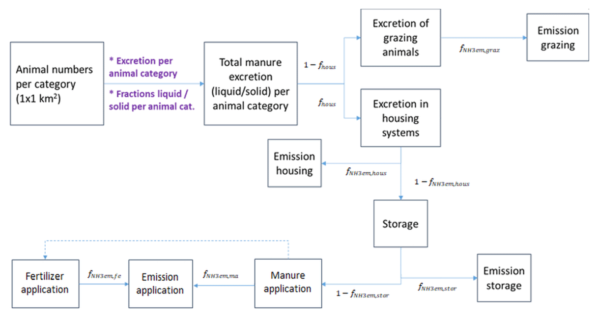
Figure 2 A schematic workflow of the NH₃ emission module in INTEGRATOR. f_hous is the fraction of total manure excretion going to housing systems. f_NH3em,graz, f_NH3em,hous, f_NH3em,stor, f_NH3em,ma and f_NH3em,fe represent emission fractions of grazing, animal housing, manure storage, manure application, and fertilizer application, respectively.

A schematic overview of the NH₃ emission module of the INTEGRATOR model is presented in Fig. 2. The emission model starts with the calculation of N excretion by multiplying the number of animals at NCU level by N excretion rate per animal per country for eight animal categories (dairy cows, other cows, pigs, laying hens, other poultry, horses, sheep and goats, and fur animals) (Kros et al., 2012). The livestock data were obtained from the FAO database at country level, using Common Agricultural Policy Regionalised Impact analysis (CAPRI) data for distribution at NUTS2 level. The data on livestock numbers of various animal categories at NUTS2 level were downscaled to a 1 km × 1 km resolution using expert-based judgment with spatial data sources on land use, slope, altitude, and soil characteristics influencing the livestock carrying (Neumann et al., 2009). A major distinction was made between grazing animals and other animals. Dairy cows, other cattle, and sheep and goats were assumed to be highly dependent on local land resources for grazing or feed production. Pigs and poultry were assumed to be held in more land-independent systems. We refer to Neumann et al. (2009) for more detailed information on livestock's downscaling. The N excreted in housing systems is the multiplication of N manure excretion and the housing fraction (f_hous in Fig. 2), while the N excreted from grazing on land is obtained by subtracting N excreted in housing systems from total N manure excretion. The total manure production is derived by subtracting gaseous emissions and leaching in housing and manure storage systems from the N excretion, while the gaseous emission from housing is calculated by multiplying N excretion by the emission fraction per housing system (f_NH3em,hous). Ammonia emission fractions for housing and manure storage are distinguished per animal type and manure type. The emissions of ammonia from agricultural land are calculated by multiplying the N input by grazing, manure application and fertilizer application with ammonia emission fractions for grazing f_NH3em,graz), manure application (f_NH3em,ma) and fertilizer application (f_NH3em,fe), respectively (Kros et al., 2012; De Vries et al., 2020). The procedure to allocate manure over grassland and different crop groups is given in Appendix B. Emission fractions for manure application (f_NH3em,ma) are distinguished for three animal types, i.e., cattle (including dairy cows, other cows, sheep and goats, horses and fur animals), pigs and poultry (laying hens, other poultry) and manure type (liquid vs. solid for cattle and pigs) (De Vries et al., 2020). Emission fractions for fertilizer application (f_NH3em,fe) are differentiated between urea-based fertilizers and nitrate-based fertilizers. Details on the various fractions are given in De Vries et al. (2020).

Finally, NH₃ emissions in each NCU are available for fertilization on 32 croplands (31 CAPRI arable crop types and grassland) with five types of manure (poultry, cattle liquid/solid, pig liquid/solid) and mineral fertilizer, as well as for grazing, housing of three animal types and manure storage of five manure types, in total 201 categories.

2.2.3 The MACC-INTEGRATOR combined inventory

We replaced the agricultural emissions in the original MACC-III inventory with the INTEGRATOR emissions, which significantly increases the level of detail. For simplification, the 31 CAPRI crop types in INTEGRATOR were aggregated into cereals, root crops, industrial crops, vegetables, grass and fodder using the Indicative Crop Classification (ICC). Consequently, there were 36 categories regarding emissions from fertilization on croplands. Grazing, animal housing, and manure storage were kept as they were, resulting in 45 categories in total in the combined emission inventory (see Fig. C1 in Appendix C).

Since the two inventories use different coordinate systems, coordinate transformation was performed to resample INTEGRATOR emissions onto the grid utilized in MACC-III. The resampling was conducted by (1) averaging the emission in one NCU evenly over the whole polygon; (2) dividing each square kilometer grid cell into 25 subpixels and calculating the coordinate of the center of each subpixel in latitude–longitude; and (3) locating the calculated coordinate of each subpixel of NCU in the MACC-III grid and assigning emission to the corresponding MACC-III grid.

It has to be pointed out that the NH₃ emission estimates from INTEGRATOR differ from the officially reported national emission totals used in the MACC-III inventory. This is because each country uses its own emission inventory methodology, whereas INTEGRATOR uses a uniform method for all countries. To assess the impact of the different spatial (and temporal) allocation and to be in line with officially reported emissions, we scaled the NH₃ emissions from INTEGRATOR with the country totals of 2010 officially reported in 2018. The scalar is computed per country per animal type, namely the division of INTEGRATOR emission and officially reported emission to EMEP.

2.3 Temporal allocator

The usual approach to characterizing the temporal variability in NH₃ emissions is to use time profiles that distribute the annual emission total in a grid cell over a year. Fixed and oversimplified temporal profiles (monthly, daily, or hourly resolved) are often used (Van Pul et al., 2009). In this section, we explicitly described the temporal allocation of NH₃ emissions from manure and fertilizer application based on the concepts of Skjøth et al. (2004), Gyldenkærne et al. (2005), and Hutchings et al. (2012). The temporal distribution functions of ammonia emission from grazing, animal housing and manure storage were taken from Gyldenkærne et al. (2005), which are presented in Appendix D.

The temporal distribution of NH₃ emission from fertilization is dependent on the timing of manure and fertilizer application on arable lands and grassland, weather conditions, as well as legislative constraints. We first followed the methodology as outlined by Gyldenkærne et al. (2005) to characterize the temporal variation of the emission strength as a function of time, temperature, and wind speed. The emission function used may be described as Eq. (1):

$$\begin{array}{}\text{(1)}& E_{i,j,k}(t,T,W)={\mathit{ϵ}}_{i,j,k}{e}^{\mathrm{0.0223}T\left(t\right)}{e}^{\mathrm{0.0419}W\left(t\right)}{\displaystyle \frac{\mathrm{1}}{\mathit{\sigma }\sqrt{\mathrm{2}\mathit{\pi }}}}{e}^{\left(\frac{(t-\mathit{\mu }{)}^{\mathrm{2}}}{-\mathrm{2}{\mathit{\sigma }}^{\mathrm{2}}}\right)},\end{array}$$

where $E_{i,j,k}$ is the emission strength after application of fertilizer k on crop j in NCU i, ${\mathit{ϵ}}_{i,j,k}$ is the annual total emission (kg ha⁻¹), T(t) and W(t) are the air temperature (^∘C) and wind speed (m s⁻¹) for the applied time step (t), μ is the day with peak emissions, and σ is the SD to represent spread and uncertainty in the application activities and emission timing.

2.3.1 The improvement of fertilization day

The first challenge was to update the estimated central day μ (the day with peak emissions) for manure and fertilizer applications. The timing of these field operations was obtained by the TIMELINES model's methodology that was developed to assess the timing of field operations, including the Julian Day of fertilization on a wide range of crops (Hutchings et al., 2012). It was calculated at the 50 km × 50 km MARS meteorological grid level in Europe (Goot, 1998). Hutchings et al. (2012) took the weather conditions over a year into account when simulating crop calendars by introducing a thermal time approach. Thermal time is the sum of the positive differences between daily mean air temperature and a base temperature and is written as Eq. (2):

$$\begin{array}{}\text{(2)}& {\mathit{\tau }}_t=\sum _{k=t_{\mathrm{0}}}^t\text{max}\left(\right({\mathit{\theta }}_k-{\mathit{\theta }}_{\mathrm{b}}),\mathrm{0}),\end{array}$$

where τ_t is the thermal time (in Celsius) over time t (day), θ_k is the daily mean air temperature at 2 m, θ_b is the base temperature (0 ^∘C), and t₀ is the starting time of calculation, 1 January. As soon as thermal time on Julian Day t reaches the reference thermal time for sowing (or harvesting), sowing (or harvesting) is considered to occur on this day. All other field operations, including plowing and manure and mineral fertilizer applications, are related to it.

We back-calculated the reference thermal times τ_{ref,sow(harv)} for various crops based on the sowing and harvesting dates provided by Hutchings et al. (2012). ECMWF meteorological data for the years between 1985 and 1995 and the respective days t_sow(harv) were inserted into Eq. (3):

$$\begin{array}{}\text{(3)}& {\mathit{\tau }}_{\text{ref,sow(harv)}}=\sum _{k=t_{\mathrm{0}}}^{t_{\text{sow(harv)}}}\text{max}\left(\right({\mathit{\theta }}_k-{\mathit{\theta }}_{\mathrm{b}}),\mathrm{0}).\end{array}$$

The period between 1985 and 1995 was selected as Hutchings et al. (2012) followed a similar proceeding based on the Crop Growth Monitoring System (CGMS) dataset and used obtained reference thermal times to calculate sowing and harvesting days for 1995 onwards. The sowing and harvesting dates derived in this paper are in good alignment with the work of Hutchings et al. (2012), as shown in Fig. E1 in Appendix E. The sowing day estimates of winter wheat and spring wheat in 2010 are shown in Appendix F Fig. F1. The timing of manure application is based on sowing dates and varies from one manure type to another. Mineral fertilizer is applied in two applications, with the first application (20 % of the annual amount) conducted 5 d prior to sowing for spring crops and at the start of the growing season for winter crops. The second application is made after 20 % of the growing season has elapsed (Hutchings et al., 2012).

We assumed that the peak of emission after application occurs at noon on the second day after the estimated central fertilization day. This is based on field experiments that show the emission from mineral fertilizers has its maximum in the first days after application (Loubet et al., 2009; Schjoerring and Mattsson, 2001; Whitehead and Raistrick, 1993). Søgaard et al. (2002) observed that half of the NH₃ emission takes place within the first 30 h. Plöchl (2001) looked into 227 experimental trials and found that 80 % of the emission was reached within two days. However, in some cases (e.g., urea applied in dry conditions resulting in slow hydrolysis), fertilizer emission may proceed for over a month after application, which is unlikely in our study area (Sutton et al., 1995). We assumed that the peak of emission after application occurs at noon on the second day after the estimated central fertilization day.

Even though the TIMELINES model indicates a single day of fertilization in an NCU, in practice, farmers certainly would not operate precisely at the same time. The central estimate of fertilization day is uncertain due to other influencing parameters such as soil conditions and the availability of machinery and labor. Also, Gyldenkærne et al. (2005) argued that there would still be variation in the timing of fertilization because it would take time for farmers to complete these operations. As a consequence, normal distribution around the central estimate was used here to characterize it.

The SD around the central value is given in a fixed number of days, since it is determined by farmers' agricultural practice (independent of the thermal sum approach) and includes a random uncertainty. Gyldenkærne et al. (2005) assumed there are four times of manure application in a year: early spring, late spring, spring–summer, and summer–fall. The SD of the spring–summer application is 16 d, while that of the remaining applications was 9 d. The SDs of the timing of the mineral fertilization applications in early spring and summer were 9 and 16 d, respectively. We made a similar assumption in this paper: for fertilizations that lie between mid-May and mid-August, the SD of the corresponding emission function is 16 d. For the remainder, the SD is considered to be 9 d.

2.3.2 The inclusion of legislative conditions

The next step is to implement legislative constraints on manure and fertilizer application. In Germany, manure application is not allowed from 1 November to 31 January on arable land and from 15 November to 31 January on grassland (Kuhn, 2017). In Flanders of Belgium, manure spreading is not allowed in the winter period from 15 October till 15 February (Vlaamse Landmaatschappij, 2016b). We expanded this period to Belgium and Luxemburg due to a lack of knowledge in these regions. As for the Netherlands, solid manure is prohibited from 1 September to 31 January, while other manures are banned between 16 September and 15 February on arable land and between 1 September and 15 February on grassland. Mineral fertilizer is prohibited from 16 September to 31 January on both grassland and arable land (Rijksdienst voor Ondernemend Nederland, 2019). Furthermore, Vlaamse Landmaatschappij (2016a) pointed out that one is not allowed to fertilize on Sundays nor when the soil is frozen or covered by snow in Flanders. Usually, frozen soil and snow cover appear outside permitted dates. The ban on fertilization outside permitted dates and on Sundays is the most significant constraint and was applied to all regions in the area of interest by setting the emission strength to zero in Eq. (1).

2.3.3 The impact of excessive precipitation

The occurrence of excessive precipitation was also accounted for since the soil can become water-saturated, negatively impacting the infiltration rate of liquid manures and the risk of strongly enhanced surface runoff. Furthermore, trafficking the wet soil surface with heavy machinery is likely impossible. We used the weekly De Martonne index to capture the characteristics related to precipitation or soil water content. The index describes the ratio between precipitation sums and average 2 m temperature (Croitoru et al., 2012). Here, the index is computed on a weekly basis to represent more real-time humidity. For weekly values, it is written as Eq. (4):

$$\begin{array}{}\text{(4)}& I_{\mathrm{w}}={\displaystyle \frac{\mathrm{52.143}{P}_{\mathrm{w}}}{T_{\mathrm{w}}+C}},\end{array}$$

where P_w is weekly total precipitation in millimeters, T_w is weekly mean temperature in ^∘C, and C is a constant (10) that ensures that negative mean temperatures do not result in negative indices. The introduction of temperature parameterizes the impact that higher temperatures will lead to faster evaporation and more effective infiltration. Baltas (2007) defined that when the annual De Martonne index exceeds 55 (namely $\mathrm{55}/\mathrm{52.143}\approx \mathrm{1.055}$ in the weekly index), the air is considered extremely humid. One example of the weekly De Martonne index time series is given in Fig. G1 in Appendix G. Kranenburg et al. (2013) used visual inspection to set up a threshold of 1.7, above which precipitation and soil water content are not suitable for fertilization, and farmers will have to postpone application. Therefore, whichever day the threshold is violated, ammonia emission is set to zero, and the remaining part of the function is moved forward by a day.

2.3.4 The finalization of the emission time profile

Moreover, a baseline in the time profile was introduced. Due to some application techniques, especially injection, manure and fertilizer stay underneath the soil for a much more extended period before ventilation. Thus, 5 % of annual emission is allocated throughout the year as a baseline to represent background emission. Since the emission time profile needed by LOTOS-EUROS has an hourly temporal resolution and a mean of 1, the temporal distribution of emission strength for fertilization was normalized to derive the final emission time profiles. Compared with the original time profiles used in LOTOS-EUROS, the newly developed ones are spatially and dynamically explicit based on land type, amounts of emission and local climatology. Examples of NH₃ emission time profiles during construction at location (47.41^∘ N, 10.98^∘ E) in latitude–longitude in 2010 are presented in Fig. H1 in Appendix H.

2.4 The LOTOS-EUROS model

The annual emission distribution and gridded hourly time profile were then imported into LOTOS-EUROS to obtain modeled surface concentrations and total columns. They were compared with satellite observations and in situ measurements for model evaluation. LOTOS-EUROS is a three-dimensional regional CTM that uses a description of the bidirectional surface–atmosphere exchange of NH₃ (Manders et al., 2017; Wichink Kruit et al., 2010). In the previous studies, the model showed good agreement with yearly averaged NH₃ measured concentrations, except that there is slight underestimation in agricultural source areas and slight overestimation in nature areas (Wichink Kruit et al., 2012). The version of LOTOS-EUROS in this study includes the labeling module by Kranenburg et al. (2013), which tracks the contribution of emission sources from specific categories to the final simulated products. The categories that we wanted to label, namely all agricultural sectors, were defined accordingly before the model runs. As a result, besides the regular outputs, the fractional contribution of each labeled category was also calculated.

2.5 Available measurements

Among the outputs of LOTOS-EUROS, surface concentration and total column calculated from three-dimensional concentration were compared with in situ measurement and satellite observations for verification. Both in situ and satellite observations have their advantages and disadvantages. Since the transport of NH₃ in the atmosphere and the reaction with other atmospheric components are rapid, its emission and deposition dynamics affect concentrations on the scale of hours to days. Ground-based stations measure NH₃ surface concentration consistently at fixed locations, and some of them have relatively high temporal resolutions (hourly or daily), which offers the possibility of studying the behavior of NH₃ emission. However, the measurements lack vertical information as most instruments only measure surface concentrations (Van Damme et al., 2015; Erisman et al., 2007). Horizontally, the setup of station networks is coarse. Representativeness is an issue since all monitoring sites' measurements will be influenced by local and regional agricultural activities and other local sources. Consequently, we need to carefully consider the stations' locations when comparing in situ measurements with simulated results. Airborne measurements have been carried out but only occasionally with limited spatial coverage during campaigns (Dammers et al., 2016; Leen et al., 2013; Nowak et al., 2010). Satellite observations have the advantage of global coverage and the possibility of calculating area-averaged observations, which are in much better correspondence to the sizes of the grid cells in regional/global models (Flechard et al., 2013). Recently, remote sensing products with a higher spatial and temporal resolution have become available for better NH₃ concentration monitoring in the lower troposphere (Clarisse et al., 2009; Van Damme et al., 2015).

2.5.1 In situ measurements

The Umweltbundesamt (UBA) research foundation sets up monitoring stations, providing governments and the public with information on air pollutants (Schleyer et al., 2013). It measures species, including NH₃, that are essential for the improvement of knowledge about air quality and climate change. The UBA also collects the data from the network of the German federal states. In addition to the German networks, the Measuring Ammonia in Nature (MAN) network monitors monthly mean values of NH₃ concentrations in Natura2000 areas in the Netherlands to detect the spatial pattern in concentration or to assess the influence of local sources (agriculture activities but also traffic) (https://man.rivm.nl/, last access: 10 August 2019) (Lolkema et al., 2015; Noordijk et al., 2020). The network aims to be representative of different habitat types, NH₃ concentration levels, area size and shape, as well as the geographical distribution (Lolkema et al., 2015). When illustrating the comparison of concentration time series, we selected several stations that are not close to local agricultural sources (as shown in Table I1 in Appendix I) so that the local influences on measurements could be minimized. Besides, by comparing all individual measurements at all available stations, the overall performance of the updated model can be determined.

2.5.2 Satellite observations

The Infrared Atmospheric Sounding Interferometer (IASI) is a Fourier transform infrared (FTIR) spectrometer that measures the thermal infrared (TIR) radiation emitted by the Earth's surface and the atmosphere. It circles in a polar Sun-synchronous orbit and operates in nadir mode. It has a wide swath width of 2 × 1100 km, which corresponds to 2 × 15 mirror positions, while the spatial resolution is 50 km × 50 km, composed of 2 circularpixel × 2 circularpixel. Each circular pixel is a 12 km diameter footprint on the ground at nadir (Clerbaux et al., 2009).

Van Damme et al. (2014) presented an improved NH₃ retrieval scheme for IASI spectra, which relies on the calculation of a dimensionless Hyperspectral Range Index (HRI). Whitburn et al. (2016) continued with HRI and introduced a neural-network-based algorithm to obtain NH₃ total columns. Van Damme et al. (2017) made some improvements by training separate neural networks for land and sea observations, enhancing thermal contrast and introducing a bias correction over land and sea and the treatment of satellite zenith angle, which resulted in the latest product artificial neural network for IASI ANNI-NH3-v2.1. As is pointed out by Van Damme et al. (2017), weighted averaging is no longer recommended in ANNI-NH3-v2.1; arithmetic mean or median is suggested if averaging has to be performed.

Regardless of the improvement of NH₃ column retrieval from satellite observations, there is still substantial variability in measurement uncertainty, varying from 5 % to over 1000 % (Van Damme et al., 2017). Measurements with small magnitude tend to have larger relative uncertainties. Due to considerable uncertainties and the requirement of clear-sky conditions, IASI data are insufficient for real-time monitoring but sufficient if used to calculate monthly or yearly average distributions. In this study, the annual mean was compared with LOTOS-EUROS output for verification. The monthly mean was calculated to investigate the feasibility of being used for validation of temporal variability. For each IASI observation, the modeled results that are closest in space and time were selected.

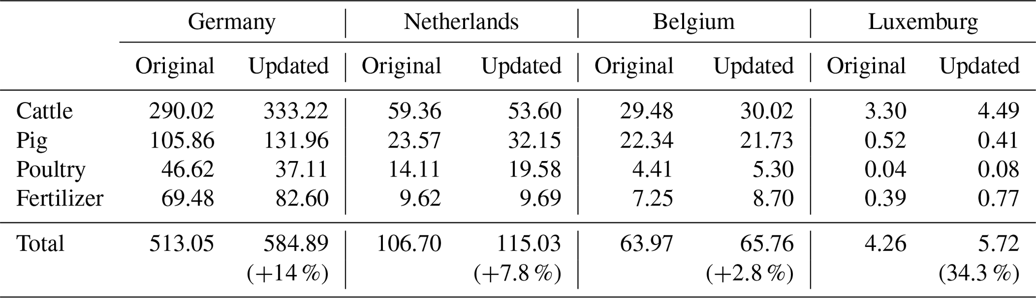
Table 1 NH₃ emission country totals (Gg yr⁻¹) for all agricultural categories and cattle, pig, poultry, and mineral fertilizer in 2010.

In this paper, we used the ANNI-NH3-v2.2R-I IASI dataset which was obtained with ECMWF ERA-Interim meteorological data and surface temperature data retrieved from a dedicated network. After the dataset was downloaded from the AERIS portal (https://iasi.aeris-data.fr/NH3R-ERA5_IASI_A_data/, last access: 20 August 2019), we only selected satellite observations with daytime overpass because daytime is the better time to measure NH₃ (Van Damme et al., 2017). Area-weighted annual mean was derived by resampling the circular footprints of IASI onto the grid used in LOTOS-EUROS. Area averaging was also applied to the calculation of the mean relative error of each grid cell. Finally, post-filtering was carried out to obtain more reliable distributions: all grid cells with less than 10 measurements were rejected.

3 Results

3.1 Comparison between MACC-III and MACC-INTEGRATOR annual emission

Because of the less detailed EMEP SNAP Level 1 categorization in the MACC-III inventory, comparisons were made at country level for cattle, pig, poultry-related emissions (the sum of housing, manure storage, and application), as well as mineral fertilizer emissions. Table 1 shows that country emission totals from the updated inventory MACC-INTEGRATOR are all larger than those from the original MACC-III inventory because it uses a different version of reported emission totals. Germany witnesses the largest positive difference in absolute value, while Luxemburg shows the most significant relative change. Compared to MACC-III, MACC-INTEGRATOR estimates more emissions from cattle and mineral fertilizer in all countries except for the Netherlands. Pig emissions in Germany and the Netherlands rise by 24.7 % and 36.4 %, respectively, while that in Belgium slightly decreases. Poultry emission drops by more than 20 % in Germany, whereas the amount increases in other countries. This implies that the scaling we applied per country based on animal types and mineral fertilizer plays an essential role. For example, INTEGRATOR estimates less agricultural emission in Germany than MACC-III, but after scaling, the combined inventory reveals the opposite trend, indicating 14 % more emission in Germany than MACC-III.

Figure 3 Maps of annual emission total (Gg yr⁻¹) for all agricultural categories and cattle, pig, poultry, and mineral fertilizer in 2010. The left panels indicate the original MACC-III inventory results, while the right panels represent the output of the updated inventory. (a, b) Emission from all agricultural sectors; (c, d) emission from cattle; (e, f) emission from pig; (g, h) emission from poultry; (i, j) emission from mineral fertilizer.

The spatial distributions of NH₃ emissions from the two inventories presented in Fig. 3a and b are the maps of annual total agricultural emissions. In Germany, the new spatial allocator assigns more emissions in the southeast near the border with Austria. The two hotspots in Bremen and the Ruhr in the original inventory merge into one located in the Ostwestfalen-Lippe region. In Schleswig-Holstein in northern Germany, the original model indicates that most of the emissions are located in the state's center. Meanwhile, the updated one indicates emissions are situated along the eastern coastline in the state. In the southeast of the Netherlands, the updated inventory allocates more emissions and smoothens the spatial details into larger blocks. After looking into NCU polygons, we found that the sizes of polygons at this location are much larger than the others. Because we evenly allocated emission within an NCU polygon over the polygon, it is possible to lose spatial characteristics, especially when a polygon has a larger size. Figure 3c and d show that cattle emission retains a similar pattern in the updated inventory, except that it is generally lower in northwestern Germany and the Netherlands. The hotspots in Overijssel and Gelderland in the east of the Netherlands disappear. By contrast, there is a much higher level of cattle emission in southern Germany bordering Switzerland and Austria. Figure 3e and f illustrate that in the updated inventory, pig emission increases in the southeast of the Netherlands and is more spread out in Nordrhein-Westfalen and Lower Saxony of Germany. Figure 3g and h demonstrate that the updated poultry emission estimate is higher in the southeast of the Netherlands, while it is lower in Lower Saxony of Germany, but to a lesser extent. It can be seen from Fig. 3i and j that emission from mineral fertilizer application only makes up a small portion of the annual totals. The patterns are quite similar, except that the emission from MACC-III sometimes shows higher values at country borders, which is not seen in MACC-INTEGRATOR. This is because they use different allocation methods: the original inventory uses proxy maps, while the updated one utilizes a balanced N fertilization approach at NCU level.

3.2 Observed and modeled NH₃ total columns

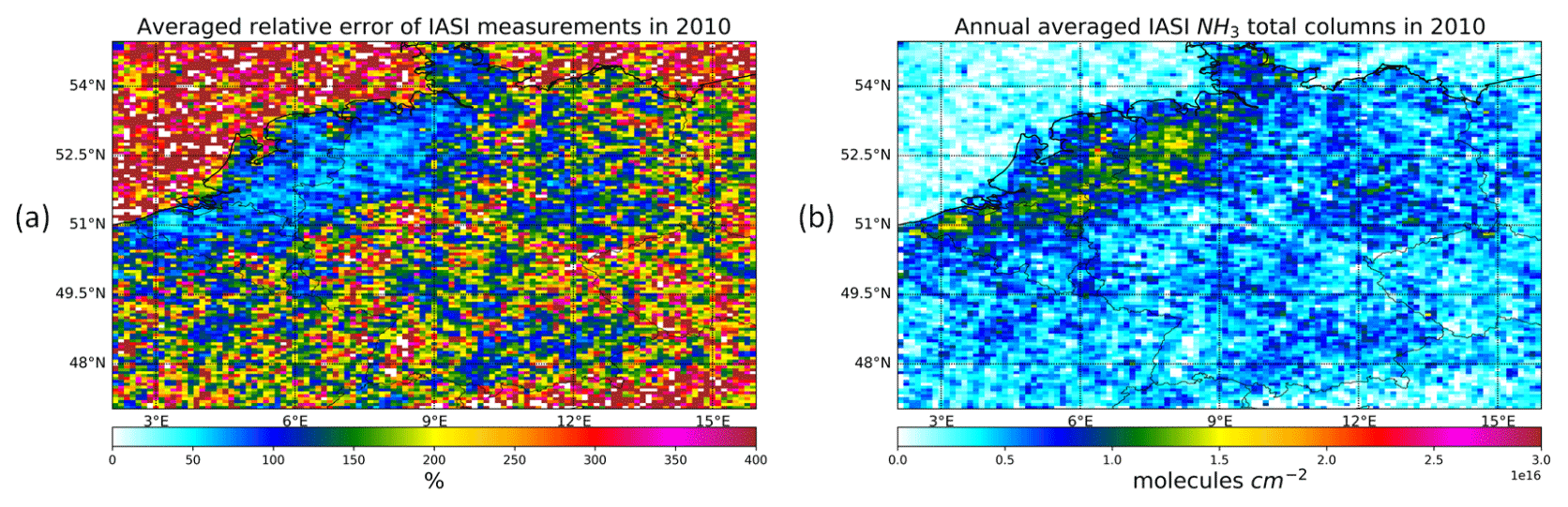
Figure 4 The map of area-averaged relative error of IASI daytime measurements in 2010 (a). The map of area-averaged total columns after filtering out grid cells with less than 10 valid measurements and an averaged relative error larger than 75 % (b).

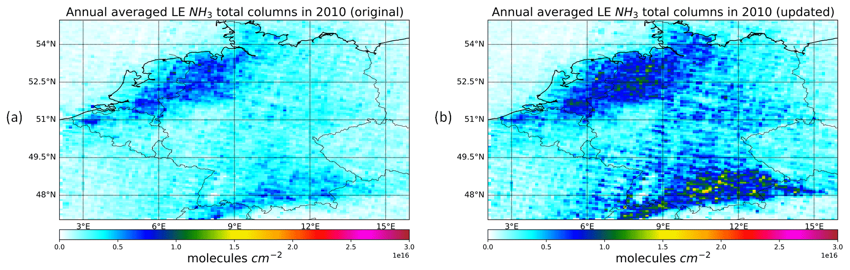
Figure 5 Simulated annual averaged total columns from LOTOS-EUROS using the original MACC-III annual emission distribution and static time profile (a) and using MACC-INTEGRATOR emission totals and updated time profiles (b).

After filtering IASI measurements, the number of valid daytime overpass measurements in each month is illustrated in Fig. J1a in Appendix J. The month in which the most valid observations (more than 7500) occurred is April, followed by July and June, in which there were nearly 6100 and 5600 measurements, respectively. The measurements in these 3 months make up more than half of the daytime measurements in the whole year. Figure J1b in Appendix J shows the spatial distribution of measurement counts over the area of interest. NH₃ is measured most frequently in western Germany, southern Germany bordering Austria, the Netherlands, Belgium and northern France. The influence of satellite footprint on the availability of data leads to the strips which are more visible in Germany and France.

The spatial characteristics of area-averaged relative error are shown in Fig. 4a. The regions with fewer measurements tend to have a higher relative error, while low errors (less than 80 %) appear in the Netherlands, Belgium, and western Germany, where many observations are available. Figure 4b represents annual area-averaged NH₃ total columns after post-filtering, which excludes gird cells that have fewer than 10 measurements. One can see that the NH₃ level is considerably high in the Netherlands, Belgium, and western Germany.

The modeled annual averaged total columns from LOTOS-EUROS simulations are shown in Fig. 5. Overall, the updated result (Fig. 5b) obtained with the updated annual emission distribution and time profiles gives a higher magnitude of NH₃ columns than the original one (Fig. 5a). Large relative differences that are more than 100 % occur mostly over Germany and the eastern Netherlands. The hotspots in the eastern Netherlands, Nordrhein-Westfalen, and Lower Saxony in the original simulations expand prominently to a much more extensive domain in the new simulation. Moreover, new hotspots are witnessed in other regions in Germany, such as Bavaria and Baden-Württemberg, close to Austria and Switzerland's borders.

Figure 6 shows scatter plots comparing IASI observations and LOTOS-EUROS estimates, with the left and right panels comparing the measurements with the original modeled result and the updated output, respectively. Figure 6a and b include all grid cells in Germany and Benelux. The simulated total columns from the original model are mostly underestimated. Meanwhile, there exist both overestimation and underestimation in the updated output. Two clusters appear in Fig. 6b, with one lying on the upper side of y=x and the other lying on the lower side. For a more straightforward illustration, comparisons were made in Fig. 6c and d for grid cells at lower latitudes (smaller than 49^∘ N) in Germany. The former shows underestimation in the south in the original model, while the latter indicates a considerable overestimation in the updated model. Moreover, Fig. 6e and f focus on the rest of the grid cells at higher latitudes and indicate that both models underestimate ammonia at these locations. Weighted linear regression was performed, with weight being inversely proportional to the square of the averaged relative error. The outcomes obtained by the new model have been improved, but both performed relatively poorly.

Figure 6 Scatter plots comparing the NH₃ annual averaged total column from IASI measurements and LOTOS-EUROS. The color of the points indicates latitude. The left panels and right panels use original and updated modeled results, respectively. (a) and (b) include all valid grid cells. (c) and (d) show grid cells with lower latitude (< 49^∘ N), while (e) and (f) focus on points with latitudes larger than 49^∘ N.

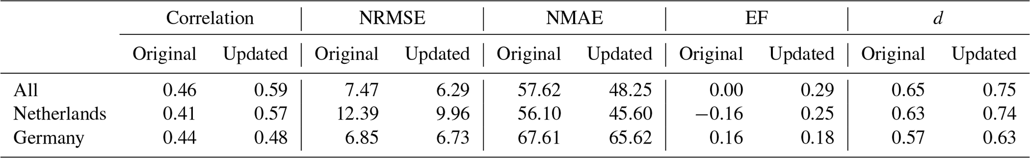
The performances of the original and updated models compared with IASI observations were investigated for all grid cells within Germany and Benelux, as well as separately in each country (Table 2). Every indicator has improved for the new modeled results. Both NRMSE and NMAE have dropped, with the largest deductions from Luxemburg. Regarding model efficiency, even though the new modeled output gives values closer to 1, they are still negative. In addition, the index of agreement witnessed the largest increase in Germany and the Netherlands.

Table 2 Performance assessment of the original and the updated model by comparing annual averaged total columns. NRMSE, NMAE, EF, and d are calculated using in situ measurements and modeled results.

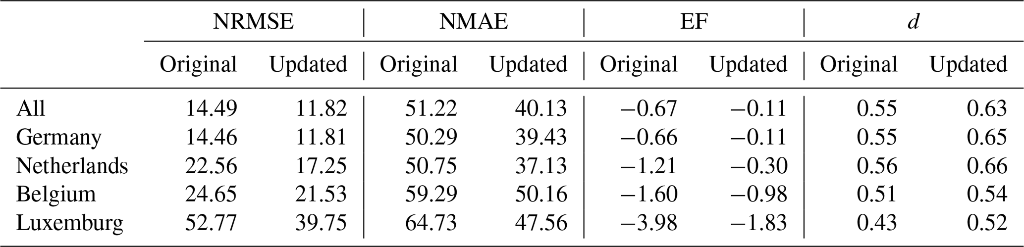
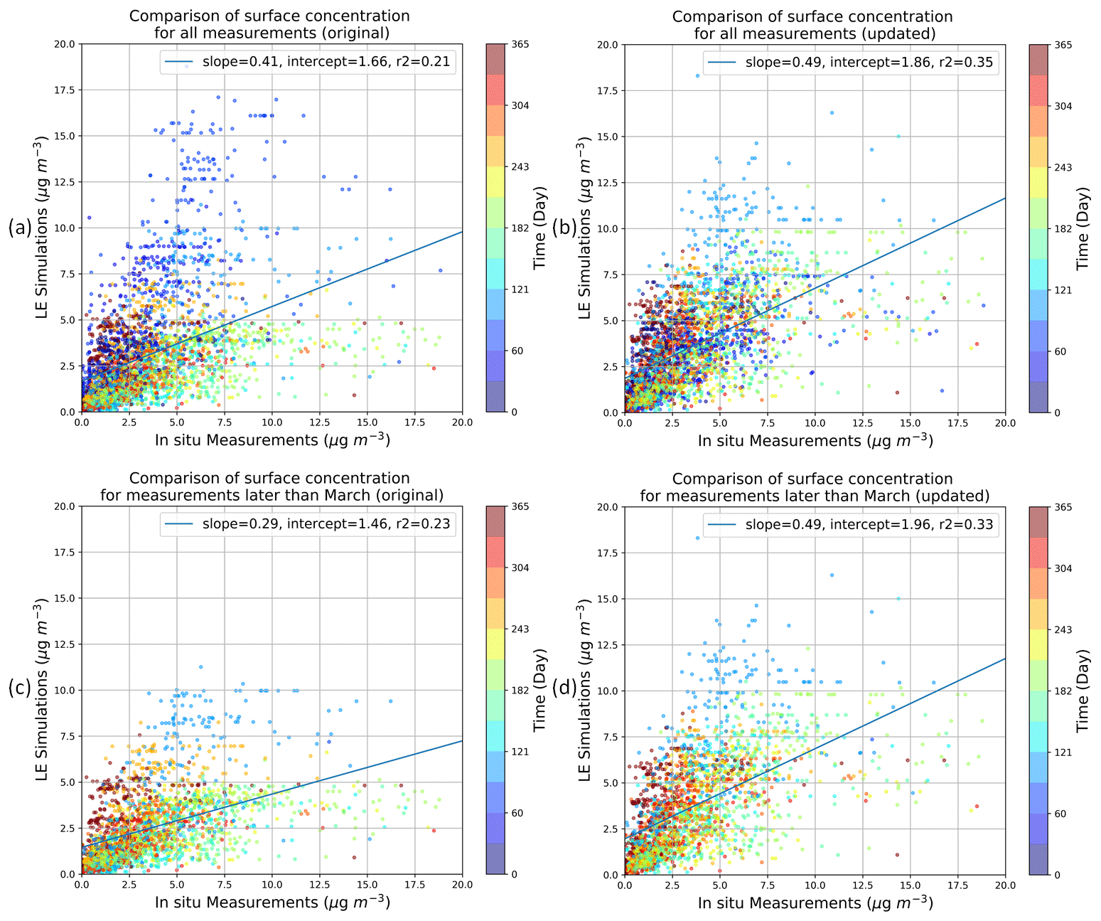
Figure 7 Scatter plots comparing NH₃ weekly or monthly averaged surface concentrations from in situ measurements and the LOTOS-EUROS model. The color of the points indicates the time (day of a year). The left panels and right panels use original and new modeled results, respectively. (a) and (b) include all measurements and corresponding simulation results, while (c) and (d) exclude the data from the first 3 months of the year.

The feasibility of verifying emission estimates by comparing weekly or monthly time series derived from IASI measurements and simulations was also investigated. However, the majority of valid data are in April, June, and July (see Fig. J1a in Appendix J). The number of valid measurements per month is insufficient for most grid cells to obtain reliable continuous time series. Consequently, two alternatives could be considered to resolve this issue. First, multiple-year averaging is required for a better trend analysis within a year. It is also possible to look at a longer time frame with coarser temporal resolution.

Table 3 Performance assessment of the original and the updated model by comparing NH₃ weekly (monthly) surface concentration. Correlation, NRMSE, NMAE, EF and d are calculated using in situ measurements and modeled results.

3.3 Observed and modeled NH₃ surface concentrations

Figure 7 provides the scatter plots between paired in situ measurements and LOTOS-EUROS simulations, showing all weekly or monthly averaged measurements (the temporal resolution depends on the measuring interval of the ground station). The updated linear regression result is better than the original one, with a slope closer to 1 and a higher R-squared value. It appears that using the updated emission model yields a more coherent estimate with reality than the original model. The midday of the sampling period is indicated through the coloring of scatter points. In Fig. 7a, most of the blue points lie on the upper side of the fitted line and y=x, which indicates that the original model usually overestimates surface concentrations (emissions) in the first 3 months of the year. In the meantime, the points in Fig. 7b are more evenly distributed with a narrower spread. If the scatter points in the first 3 months are excluded, as is shown in Fig. 7c and d, the linear regression result is worsened dramatically. By contrast, filtering out measurements in the beginning months does not impact the comparison between the new modeled results and measurements. Both slope and R-squared almost remain the same, which implies that the updated model's performance is more robust and stable.

Once again, the four indicators and correlation coefficient were calculated to determine the performance of the original and updated models (Table 3). All indices illustrate that the updated model has improved surface concentration estimates. The improvement in the Netherlands is much larger than that in Germany. The reason might be that the setup of ground stations is more consistent in the Netherlands. The locations of the Dutch stations are in the nature areas, making them more representative of the overall emission temporal variation of a grid cell.

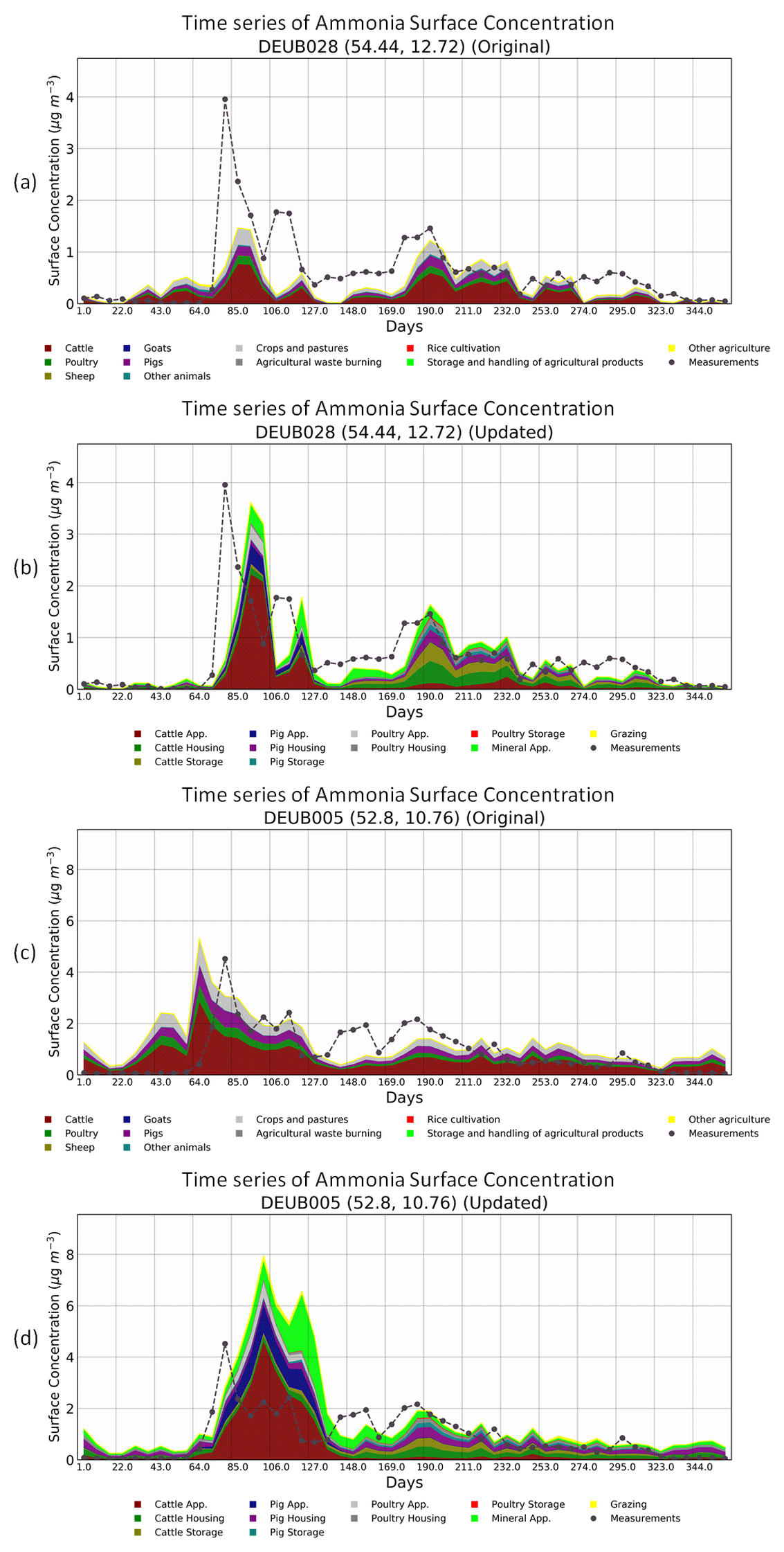
Figure 8 Comparison of surface concentration measurements within the EMEP network and simulated surface concentrations from original and updated modeled annual emission and time profiles: (a) in situ measurements vs. the original modeled output at station DEUB028; (b) in situ measurements vs. the updated modeled output at station DEUB028; (c) in situ measurements vs. the original modeled output at station DEUB005; (d) in situ measurements vs. the updated modeled output at station DEUB005.

Figure 8a and b show the change in modeled surface concentration time series for Station DEUB028 in Zingst, Mecklenburg-Vorpommern, Germany. The station is located in an agriculturally active region with cereals, industrial crops, and animal housing. As can be seen in Fig. 8a, the original model does not correspond to the measurements well. There is almost no NH₃ measured before Julian Day 64, but the original model estimates that there are two peaks on Days 38 and 59. Besides, the first two peaks in the measurement on Julian Days 80 and 110 are not captured by the original model. By contrast, the updated model manages to simulate these two peaks, even though they are slightly delayed by 10 d. The first and larger peak of the two in spring is mainly explained by cattle manure application, followed by pig and poultry manure application, and mineral fertilizer contributes to a lesser extent. In the summer between Days 150 and 275, the new modeled result also does a good job distributing NH₃ emission temporally, with animal houses, cattle storage and mineral fertilizer application dominating NH₃ emission.

A similar situation applies to Station DEUB005 in Lüder-Langenbrügge, as shown in Fig. 8c and d. We can see from Fig. 8c that the original model again allocates substantial emissions at the beginning of the year. The updated model improves the estimates a lot: even merged peaks from spring mineral fertilizer and manure application are detected. However, there still exist two issues. One is that the peaks in spring between Days 64 and 140 are overestimated. The other one is that the whole time series is delayed by 5 d. A possible reason for the delay of fertilization emission is that the reference temperature sum in TIMELINES to estimate fertilization day is too large at this location. Another cause could be that the threshold of the De Martonne index (1.7) is too low at this location. Some days in February are considered to have excessive rain, so the whole curve is shifted to the right direction of the x axis.

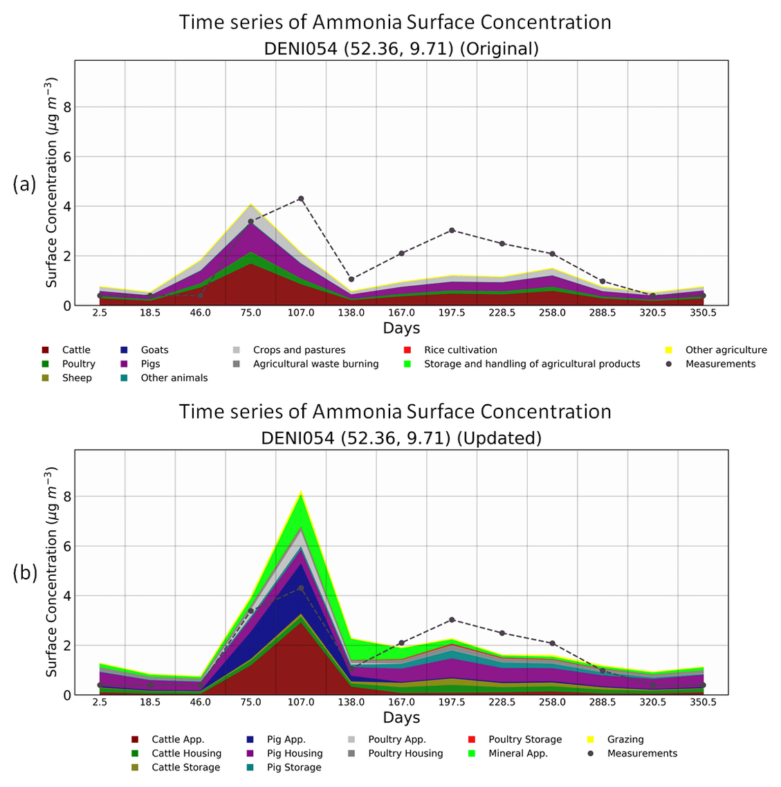
Figure 9 Comparison of surface concentration measurements within the EMEP network and simulated surface concentrations from original and updated modeled annual emission and time profiles at station DENI054. (a) In situ measurements vs. the original modeled output; (b) in situ measurements vs. the updated modeled output.

Another station in the region of Hanover, Lower Saxony, is demonstrated in Fig. 9. The measurements at this station only have a monthly temporal resolution. The updated model has shown much better correspondence to measurements than the original one, except that the average surface concentration in May is almost 50 % higher. Figure 9b is able to point out that most of the agricultural activity at this location is related to fertilization, among which cattle and pig manure applications have dominance. Thus, the overestimation in spring is probably linked to cattle or pig manure application. There are two possible contributions to this behavior. One is the emission fractions used in INTEGRATOR. The INTEGRATOR model uses country-dependent emission fractions, which have been updated and detailed through others' studies. However, they do not account for differences in manure characteristics, climatology, and soil properties. Another reason is the way of resampling emission from NCU polygons to the grids in LOTOS-EUROS, which leads to misallocation of emission to places without any sources. Last but not least, Lower Saxony is one of the states in Germany which has the highest density of livestock in the country. INTEGRATOR model calculates NH₃ emission based on proxy maps of animal number and excretion input, without considering the fact that manure from this high-production region could be transported to other areas where manure is in demand. This will also lead to an overestimation in regions with excessive livestock excretion.

4 Discussion and conclusions

4.1 The comparison with in situ surface concentration measurements

The comparison of surface concentration mainly casts light on the quality of the temporal allocator. Regarding the newly developed temporal allocator, we made modifications to the parameterization proposed by Skjøth (2004, 2011) and Gyldenkærne (2005), which accounts for the agricultural activities and their differences, based on meteorological variables as well as the ventilation and heating inside stables. The first modification is that subsectors of manure/fertilizer application emission were created to adapt to INTEGRATOR's categorization. Secondly, emission peak μ in Eq. (1) was updated by the estimated fertilization day from TIMELINES. Lastly, legislative constraints and the impact of excessive precipitation were also implemented.

The time series of surface concentrations from the updated model show better alignment with in situ measurements than those from the original model, making it possible to detect the NH₃ temporal variability brought by various agricultural activities. This is achieved by making adjustments to the method in Gyldenkærne et al. (2005) using TIMELINES, implementing legislative constraints, and including the impact of excessive precipitation. Nevertheless, there are occurrences of inconsistency.

First, the modeled time series could be delayed with respect to in situ measurements. A possible reason is that the reference temperature sum in TIMELINES to estimate fertilization day needs correction. Agricultural models, including TIMELINES, usually work from the perspective of maximizing the efficiency of nitrogen use. However, farmers are likely to choose to apply manure and mineral fertilizer when labor and machinery are both available and are unlikely to finish manure application in one day on the farmlands. This leads to the inaccuracy between the fertilization day estimate and reality and an extended manure application period. Moreover, the TIMELINES model heavily depends on the empirical data on sowing and harvesting dates currently used within CGMS to calculate the thermal time thresholds. The data need updates and are limited regarding the variety of crops, making it capable of simulating the timing of field operations for some but not all arable crops at different locations across Europe. Consequently, a more thorough analysis is needed to refine the relationships between various field operations (Hutchings et al., 2012). There are other factors related to the timing of fertilization. For example, soil moisture, workability, and trafficability were neglected in TIMELINES, but they might affect the prediction of plowing and sowing. In addition, solid manure applications for spring crops could be made in fall of the previous year. Another reason for the delay could be the threshold of the De Martonne index (1.7), which was decided with a visual inspection for Flanders by Kranenburg et al. (2013) and expanded to the whole area of interest. When the threshold is too small, the time profile will be delayed because precipitation is too often considered to be excessive for fertilization operations. Further improvement of the De Martonne index algorithm is needed to account for regional differences. More studies about the De Martonne index should be done to correlate excessive precipitation and its impact on agricultural practices.

Furthermore, sometimes the magnitude of surface concentration is not in accordance with measurement, or the time series completely mismatches measurements. This could be caused by emission reallocation from NCU to the LOTOS-EUROS grid as well as the restricted spatial representativity of measurement locations. During the resampling of emissions from NCU level to the LOTOS-EUROS grid, emission estimates within an NCU from INTEGRATOR are evenly distributed all over the polygon, regardless of the actual locations of crops, animal houses, and manure storage facilities. In addition, some NCUs are composed of multiple disconnected polygons, within only some of which a particular crop, animal house, or manure storage is present. Hence, emissions are wrongly allocated to areas without any sources. Besides, spatial characteristics such as hotspots will be smoothened out for NCU polygons of larger sizes. Therefore, high-resolution crop maps can help allocate emission from fertilization inside polygons to where arable land and grassland appear, and detailed information on animal housing locations can transform housing emissions into point emissions. What is more, in situ measurements represent the NH₃ emission characteristics of a point source, but the spatial resolution of the updated model is around 7 km × 7 km, which is relatively coarse. A station next to animal houses or manure storage facilities will result in a constant high level of NH₃ over the year, while a station next to farmlands will be highly affected by agricultural operations on the farmlands. Therefore, stations in remote areas are more representative of a broader region. This is why the updated model performs better at Dutch stations than at German stations (Table 3). MAN stations are set up to measure nature emission of ammonia, so their measurements represent better the emission variability in the grid cells. However, there are always stations next to sources given the size of the country. Ideally, in order to accurately verify the temporal allocation of emission from fertilization and housing, the spatial resolution should be increased with the help of a detailed crop map and animal housing information so that grid cells can represent local agricultural activity more.

As a result, a detailed crop map is a key to the improvement of ammonia emission estimates. Inglada et al. (2015) assessed the state-of-the-art supervised classification methods and produced more accurate crop-type maps with high-resolution multi-temporal optical imagery from SPOT4 (Take5) and Landsat 8. Surface reflectance, the normalized difference vegetation index (NDVI), the normalized difference water index (NDWI) and brightness were chosen as features, and random forest and support vector machine (SVM) were selected as classifiers. Belgiu and Csillik (2018) proposed a time-weighted dynamic time warping (TWDTW) method that uses NDVI time series obtained by Sentinel-2 data for classification. It was proven to be more efficient in terms of computational time and less sensitive concerning the training samples, which is essential for regions where inputs for training samples are limited. Besides Sentinel-2 optical images, Giordano et al. (2018) also included Sentinel-1 radar measurements for crop classification using the complementarity between the multi-modal images, because Sentinel-1 radar images allow more information to be obtained where Sentinel-2 suffers from cloud cover. We will make use of the above methods to obtain crop maps with high spatial resolution. The maps will be used to update manure distribution according to N demand of different crops and subsequent ammonia emissions. They are helpful in allocating emission from manure and fertilizer application in a more precise way.

4.2 The comparison with IASI total column data

The quality of the modeled annual averaged total column relies on the assumption that the spatial distribution of the NH₃ emission in LOTOS-EUROS closely represents reality. The temporal distribution is also of great importance because only modeled columns at overpass time were selected for averaging.

There are large inconsistencies in the comparison between IASI observations and the modeled results from both the original and updated models. One reason for the inaccurate emission allocation could be that land use data and local agricultural activity inputs such as animal numbers and N excretion in INTEGRATOR are inaccurate. Local agricultural activity data are more accessible in countries like the Netherlands, Denmark, and Portugal, and land use data can be updated with a detailed crop map as discussed previously to achieve more accurate N demand estimates, manure and fertilizer distribution, and subsequent ammonia emission. Another factor that could cause spatial inconsistencies is the emission fractions used in INTEGRATOR. Emission fractions are nation-wide averages that describe the linear relation between emission and N input (excretion in animal housing and manure storage, applied manure and fertilizer), but in reality, they could vary from region to region due to application methods, manure properties, soil properties, and weather conditions. Huijsmans has studied those impacts for both arable land and grassland (Huijsmans, 2003; Huijsmans et al., 2001). He defined the formula to describe the relationship between NH₃ volatilization rate and the method of application and incorporation, total ammoniacal nitrogen (TAN) content of the manure, manure application rate, wind speed and ambient temperature. Additionally, the empirical modeling of the emission process is carried out by RIVM and WUR using the Volt'air approach (Huijsmans et al., 2014). Preliminary results show that the variations of weather conditions over the past 20 years lead to different emission fractions per month, and soil and manure characteristics also influence emission fraction. As a result, emission fraction differs at farm scale, contributing to an inhomogeneous emission fraction on a regional or national scale. Therefore, there are two steps for improvement in terms of land use, local agricultural activity data and emission fraction. In the short term, we will implement detailed land use and local activity data for the Netherlands, Denmark, and Portugal and investigate the difference brought by the refinement of the input. Next, a meta-analysis will be performed for the parameterization of spatially and temporally explicit emission fractions, taking into account local climatology, soil properties, fertilizer characteristics and application method.

A possible source of overestimation in lower latitudes and underestimation in higher latitudes in Germany is the neglect of possible manure transport. INTEGRATOR assumes that the emissions from a certain animal, including housing, storage and manure application, occur where the animal is located, ignoring manure transport from regions with excessive manure to those with shortages. The role of manure transport is more significant when there is a lot of animal livestock. Hendriks et al. (2016) looked into manure transport data in Flanders and found that the manure transport data account for roughly one-third of the amount of manure used in Flanders each year, while the remaining two-thirds consist of manure that farmers apply on their own land. Hansen-Kuhn et al. (2014) showed that southern Germany is one of the areas in the country which has the highest density of cattle and pig livestock. It is likely that the neglect of manure transport contributes to the overestimation in the lower latitudes. Therefore, manure transport data can be used as a proxy to improve the spatial distribution, and the pattern of manure transport can additionally help construct the temporal pattern of NH₃ emissions from manure application, under the assumption that manure is applied to the fields on the day of transport.

Moreover, the uncertainty in IASI measurements also has an impact on the comparison. Dammers et al. (2016) found that the validity of the IASI product is quite limited because the satellite retrievals are biased. The retrieval of NH₃ columns from IASI is still an ongoing process, with a few studies having examined the quality of the products. Further development and validation of the IASI retrieval are very much needed for understanding of the satellite's product. It remains poorly validated, with only a few dedicated campaigns performed with limited spatial, vertical or temporal coverage. The key finding of the previous studies on the retrieval is that vertical profiles of NH₃ distribution have lots of uncertainties and need to be improved. Dammers et al. (2016) suggested that tower measurement campaigns are crucial for a better understanding of the vertical profile. Li et al. (2017) showed that there is an apparent seasonal variation in the vertical distribution of NH₃ and that the slope of the NH₃ concentration gradient varies throughout the year, with relatively high NH₃ ground concentrations during winter. His reasoning was that the boundary layer is shallower in winter, which will potentially trap NH₃ emissions and reduce NH₃ concentrations higher up the column. As a result, IASI could miss high NH₃ ground concentrations in winter because of the lack of sensitivity to the lower parts of the boundary layer. By contrast, most of the measurements used in this paper to calculate annual average are in April, June and July, in which weather is relatively warmer and the boundary layer is thicker, especially during clear-sky daytime conditions. Recently, new products have become available, making it possible to cross-check results among satellites. Cross-track Infrared Sounder (CrIS) is one of the new products that deserve attention, having the advantage of acquiring more explicit information on the sensitivity of the satellite (averaging kernel).

4.3 Conclusions

In summary, this paper is an attempt to build a new NH₃ emission model which is composed of a spatial allocator and a temporal allocator. The spatial allocator provides more spatial details and can distinguish various agricultural sectors, including crop types, fertilizer types, animal houses and manure storages. The distribution of annual emission obtained from MACC-INTEGRATOR demonstrates more emissions overall, with country totals 14 % higher in Germany and 6.6 % higher in Benelux. Extra new hotspots appear in southeastern Germany, while the spatial characteristics in the east of the Netherlands are smoothened due to the allocation algorithm. The temporal allocator is spatially explicit and dynamic based on land use, local climatology, and legislative constraints. The labeling module of LOTOS-EUROS helps to track back the emission sector of the modeled NH₃ surface concentration and total columns for better interpretation and future improvement. Despite the limitations in modeling and data for validation, LOTOS-EUROS performed better with the updated emission products, especially in the representation of the temporal behavior of NH₃ concentrations. Comparison between updated modeled results and observed NH₃ levels shows much better correspondence and more robust performance; especially the temporal variability is captured better as the new methodology successfully differentiates regional variability in seasonality in NH₃ emissions. When reliable and detailed input datasets are available, and the methodology is further improved as described, we can expect to extend this approach to Europe.

Appendix A: Statistical indices used to assess the performance of the models

To evaluate the performance of the updated model and compare it with that of the original model, we calculated the normalized root mean square error (NRMSE), the normalized mean absolute error (NMAE), the model efficiency (EF) and the index of agreement between the modeled results (predictions) and measurements.

The root mean square error of n predicted values of a regression's dependent variable, with ${\widehat{y}}_i$ being the ith prediction and y_i being the ith estimate, is computed as the square root of the mean of the squares of the deviations:

$$\begin{array}{}\text{(A1)}& \text{RMSE}=\sqrt{{\displaystyle \frac{{\sum }_{i=\mathrm{1}}^n({\widehat{y}}_i-y_i{)}^{\mathrm{2}}}{n}}}.\end{array}$$

The NRMSE indicates RMSE in a relative sense, by dividing RMSE by the difference between the maximum and minimum observed values:

$$\begin{array}{}\text{(A2)}& \text{NRMSE}={\displaystyle \frac{\text{RMSE}}{y_{\text{max}}-y_{\text{min}}}}.\end{array}$$

The normalized mean absolute error (MAE) is interpreted as the average absolute difference between y_i and ${\widehat{y}}_i$, with reference to the mean of observations:

$$\begin{array}{}\text{(A3)}& \text{NMAE}={\displaystyle \frac{{\sum }_{i=\mathrm{1}}^n\left|{\widehat{y}}_i-y_i\right|}{n}}/\overline{y}.\end{array}$$

The model efficiency coefficient is used to illustrate predictive power. It can range from −∞ to 1. An efficiency of 1 indicates a perfect match of simulations to observations (Ritter and Muñoz-Carpena, 2013). The closer the model efficiency is to 1, the more accurate the model is.

$$\begin{array}{}\text{(A4)}& \text{EF}=\mathrm{1}-{\displaystyle \frac{{\sum }_{i=\mathrm{1}}^n({\widehat{y}}_i-y_i{)}^{\mathrm{2}}}{{\sum }_{i=\mathrm{1}}^n(y_i-\overline{y}{)}^{\mathrm{2}}}}\end{array}$$

Last but not least, the index of agreement (d) statistic was also employed, which represents the ratio of the mean square error and the potential error (Willmott, 1981). The agreement value of 1 indicates a perfect match, and 0 indicates no agreement at all. However, it is overly sensitive to extreme values due to the squared differences (Willmott, 1981).

$$\begin{array}{}\text{(A5)}& d=\mathrm{1}-{\displaystyle \frac{{\sum }_{i=\mathrm{1}}^n({\widehat{y}}_i-y_i{)}^{\mathrm{2}}}{{\sum }_{i=\mathrm{1}}^n(\left|{\widehat{y}}_i-\overline{y}\right|+\left|y_i-\overline{y}\right|{)}^{\mathrm{2}}}}\end{array}$$

Appendix B: Methodology to allocate manure application over grassland and arable crop groups

In the INTEGRATOR model, manure is distributed over grassland and different crop groups using various allocation rules. Manure produced by grazing animals and in housing systems by sheep and goats all enters grassland. For other manure, a fraction is applied to arable land, and the remaining fraction is applied to grassland/fodder crops, distinguishing (i) liquid manure of dairy cattle, other cattle and pigs, (ii) solid manure of dairy cattle, other cattle and pigs and (iii) poultry manure. For the distribution of manure application on arable land, we distinguish three arable crop groups with (i) a relatively high use of manure (sugar beet, barley, rape, and soft wheat), (ii) an intermediate use of manure (potatoes, durum wheat, rye, oats, grain maize, other cereals including triticale, and sunflower), and (iii) low use of manure (fruits, citrus, olives, oil crops, citrus, grapes and other crops) using weighing, based on Velthof et al. (2009). Finally, no manure is allocated to dry pulses and rice, fiber crops, other root crops and vegetables.

As the last step, mineral fertilizer is distributed over crops on country level using a balanced N fertilization approach.

1. The total N demand in a NUTS 2 region is calculated as the sum of N in harvested products and in crop residues. The N in harvested crops is calculated from the crop yield and the N content in crop yield. The yields of arable crops for each country were derived from FAOSTAT on a country basis, and the N contents of harvested crop products were based on the literature. The N in crop residues is calculated by dividing the N removed in harvest by an N index.

2. The fertilizer N demand of each crop was calculated by subtracting the non-fertilizer N input from the total N demand and then divided by the N use efficiency (NUE).

3. The N fertilizer estimates for each NUTS 2 region were aggregated at country level and compared with reported country-level N fertilizer consumption. Scaling factors (the ratio of the known and calculated country-level N fertilizer consumption) were then applied to ensure consistency.

Appendix C: Fertilizer and crop categorization in the MACC-INTEGRATOR combined emission inventory

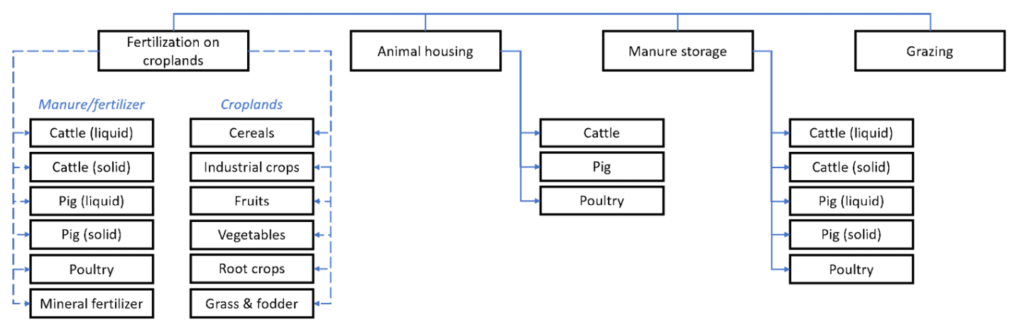
Figure C1 Categorization in the MACC-INTEGRATOR combined emission inventory. There are six fertilizer types and six crop types, resulting in 36 categories regarding fertilization. Together with three animal housing types, five manure storage types, and grazing, there are 45 categories in the new NH₃ emission model.

Appendix D: Calculation of the temporal variation of ammonia emission due to grazing, animal housing and manure storage

For the temporal variation of NH₃ emission from fertilization on grassland, we used the parameterizations of Skjøth et al. (2004) for Danish conditions using a Gauss function as given below:

$$\begin{array}{}\text{(D1)}& \left\{\begin{array}{l}{F}_{\text{grass}}=E(x,y)\cdot e^{\mathrm{0.0223}T\left(t\right)}{e}^{\mathrm{0.0419}W\left(t\right)}\cdot \frac{e^{\left(\frac{(t-\mathit{\mu }{)}^{\mathrm{2}}}{-\mathrm{2}{\mathit{\sigma }}^{\mathrm{2}}}\right)}}{\mathit{\sigma }\sqrt{\mathrm{2}\mathit{\pi }}},\\ \mathit{\mu }=T_{\text{sum1400}}(x,y)+\mathrm{4},\end{array}\right.\end{array}$$

where t is the actual time of the year, E(xy) is the total emission from fertilization on grassland within a grid cell, μ is the mean value for the Gaussian distribution, T(t) is the air temperature in ^∘C, and W(t) is the wind speed (m s⁻¹) for the applied time step (t). μ is the Julian Day on which the thermal sum reaches 1400, except that the starting day of thermal time calculation is 1 March, instead of 1 January. μ depends on local climatology, so it differs from grid cell to grid cell. σ is the spread of the Gauss function and is equated to 60 d, which means that grazing occurs in a relatively long period of time.

Regarding emissions from grazing on grassland, it is generally dependent on the release time of the cattle, the availability of grass, and the length of the growing season (Gyldenkærne et al., 2005). The availability of grass is then primarily a function of precipitation, soil humidity, soil fertility, and fertilization. For a region that has a relatively even distribution of the precipitation during summer, such as the study area in this paper, Gyldenkærne et al. (2005) suggested that a model following grass growth could be used to represent the characteristics of grazing emissions. Therefore, as in the work of Skjøth et al. (2004), here emission from grazing is assumed to follow the same pattern as grown grass in Eq. (D1).

Emission patterns from animal housing and manure storage are based on Skjøth et al. (2011) and Gyldenkærne et al. (2005) as given below:

$$\begin{array}{}\text{(D2)}& \left\{\begin{array}{l}{\text{Fkt}}_i=\frac{E_i(x,y)}{{\text{Epot}}_i(x,y)}\cdot \left(T_i\right(x,y){)}^{\mathrm{0.89}},T_i(x,y)\ge T_{\text{boundary}}\\ T_i(x,y)=\left\{\begin{array}{ll}\mathrm{18}+\mathrm{0.77}\cdot \left(T(x,y)-\mathrm{12.5}\right),& \text{Insulated houses}\\ T(x,y)+\mathrm{3},& \text{Open houses}\\ T(x,y),& \text{Manure storage}\end{array}\right.\end{array}\right.\end{array}$$

where i refers to the index (1–3) of insulated housing, open housing and manure storage, respectively. x, y are the coordinates of the emission grid. E_i(xy) represents the emission for the corresponding agricultural sector within the grid cell. Epot_i(xy) is a constant emission potential scaling factor for a given grid cell and can be neglected for simplicity (Elzing and Monteny, 1997). T_i(x,y) is temperature function, which is different for housing, open housing and manure storage. T(x,y) is the 2 m temperature at the given location and is obtained from the ECMWF data portal. It can be seen from Eq. (D2) that open houses and manure storage have almost the same emission pattern, except that the indoor temperature in open houses is 3 degree higher than the outside temperature used for manure storage (Gyldenkærne et al., 2005). T_boundary represents the lower boundary condition for temperature in animal housing and manure storage, below which emission is set to a constant level, and they are 18, 4, and 1 degree, respectively.

Pigs and poultry have a high lower critical temperature (LCT) between 6 and 20 degrees, below which an animal must expend additional energy to maintain normal body temperature and essential body functions. So in colder climates, they are usually kept in insulated buildings with forced ventilation to maintain a fixed temperature throughout the year (Seedorf et al., 1998a). By contrast, cattle have a very low LCT and are therefore often kept in open barns (Seedorf et al., 1998b). However, there still might be some insulated cattle barns with forced ventilation in colder climates (Gyldenkærne et al., 2005). Consequently, the function for forced ventilation is used to represent the temporal variation of pig and poultry housing emission, while the mean of functions of insulated houses with forced ventilation and open houses is calculated to characterize cattle housing emission. In terms of manure storage, it is assumed that the emissions from manure storage of all animal types have the same pattern.

Appendix E: Comparison of sowing day estimates

Comparisons between sowing days calculated in this study and by Hutchings et al. (2012) were made for verification. Figure E1 depicts an example of the calculated sowing days of potatoes. Only the dates for years between 1985 and 2000 are selected for comparison because Hutchings et al. (2012) used predicted temperature data for years after 2000. The sowing days are in good alignment, with only a few outliers away from line y=x.

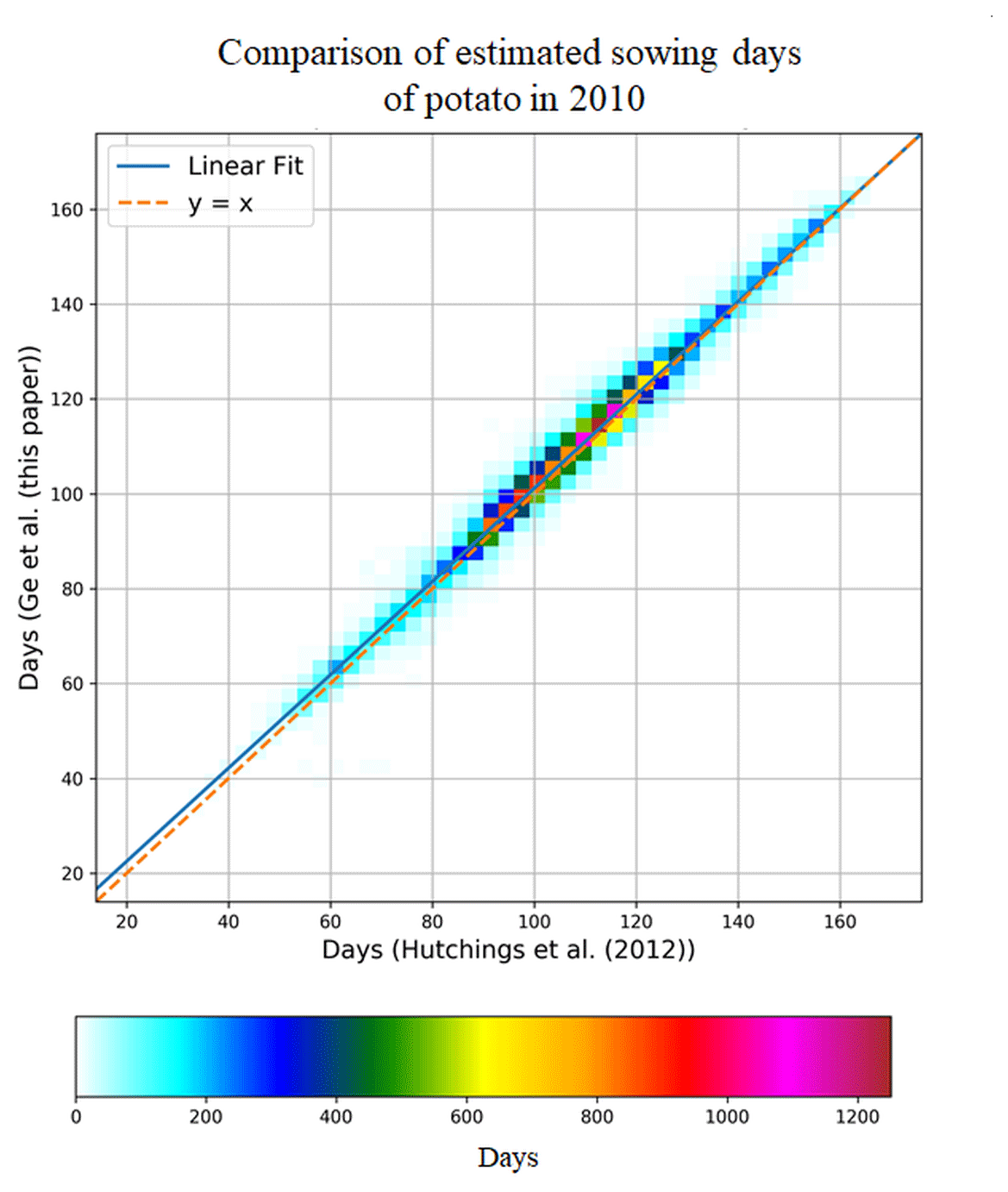
Figure E1 The density plot comparing sowing day estimates of potato between 1985 and 1995 by Hutchings et al. (2012) (x axis) and in this study (y axis).

Appendix F: Spatial variation in sowing day estimates for winter wheat and spring wheat

Figure F1 shows that the sowing days of winter wheat and spring wheat generally have opposite trends. For winter wheat, even though the differences between daily mean temperature and the base temperature are larger in the south, the greater reference thermal sum makes it take a longer time to reach this thermal sum, whereas for spring wheat, the reference thermal sum in the south is less than that in the north, resulting in an earlier sowing day than in the north.

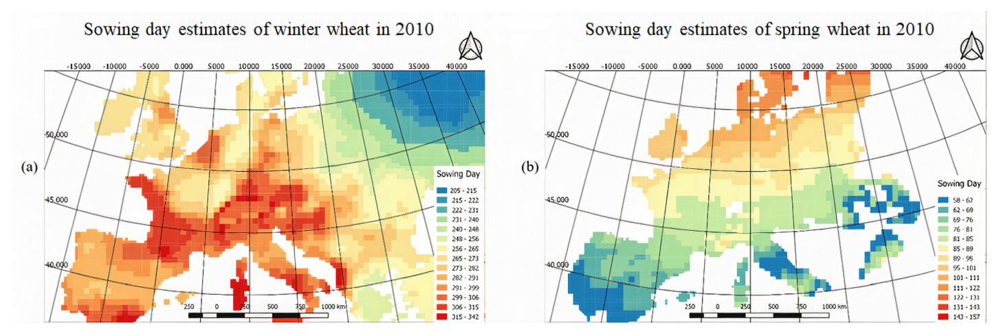
Figure F1 Two examples of estimated sowing days over Europe from the TIMELINES model for winter wheat (a) and spring wheat (b) in 2010.

Appendix G: Time series of the weekly De Martonne index

Figure G1 shows that the weekly De Martonne index at location coordinate (48.98, 8.14) approximately ranges between 0 and 6.5 in 2010. High indices are observed around Day 30 before the first spring application period as well as at the end of the year. On these occasions, the index reaches values well above 3.

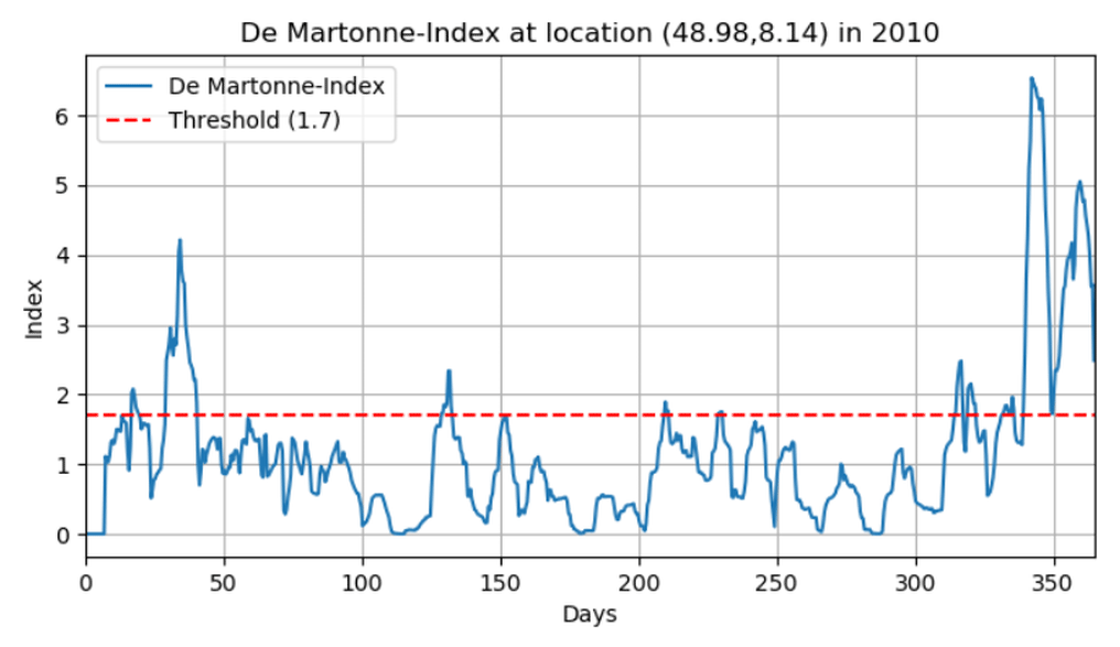
Figure G1 An example of the time series of the weekly De Martonne index at (48.98, 8.14). A threshold of 1.7 is determined, above which precipitation is considered to be excessive.

Appendix H: Examples of ammonia emission time profiles

Examples of NH₃ emission time profiles during development at the location (47.41^∘ N, 10.98^∘ E) in latitude–longitude in 2010 are presented in Fig. H1. The left panels represent time profiles of the application of cattle liquid manure on cereals, while the right panels demonstrate that of pig liquid manure application on grass and fodder. The four rows indicate the four phases during the development of the time profiles. First and foremost, the initial emission time profiles (first row) in all the panels were obtained using fertilization day estimation from TIMELINES and the emission function in Eq. (1), taking into account local climatology including temperature and wind speed. Subsequently, the emission strengths of Sundays were set to baseline since manure and fertilizer applications were prohibited, as is shown in the second row. Furthermore, in the third row, prohibition on fertilization after late fall and before early spring (exact dates vary from country to country) did not affect the time profiles in the left panels since the emission function lies within the period where fertilization is allowed. However, for the right panels, part of the third peak exceeded the last allowed date for application. Thus, the part outside the application ban was cut out, and the rest of the peak was scaled accordingly. Finally, the impact of excessive rain on emission was accounted for in the last row. On each day where the De Martonne index exceeded the threshold 1.7, the emission curve before this day remained as it is, while the rest was shifted to the next possible day. It is possible that in the final time profile, emission lies slightly outside the permitted period for fertilization. However, it is allowed under the assumption that the government allows a delay in manure and fertilizer application due to weather.

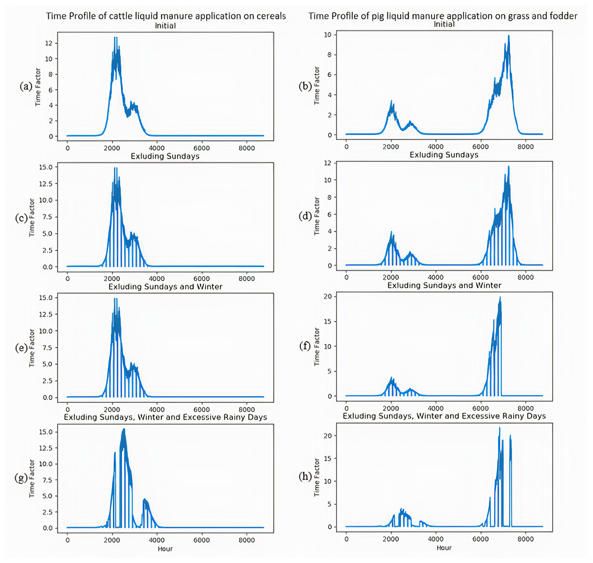
Figure H1 Two examples of the NH₃ emission time profile during the four phases of development at location (47.41, 10.98) in latitude–longitude: cattle slurry application on cereals (a, c, g, e) and pig liquid manure application on grass and fodder (b, d, f, h).

Appendix I: Land use information of the selected in situ measurement sites

Table I1 Information on the selected in situ measurement sites.

Appendix J: Monthly statistics and spatial distribution of the number of valid IASI measurements

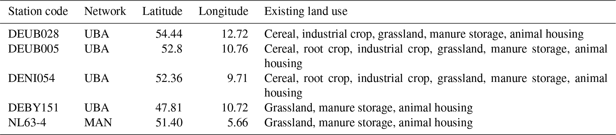
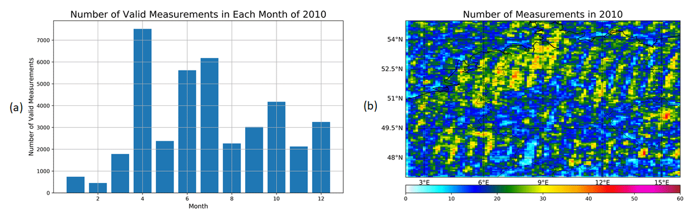
Figure J1 The bar plot of the number of IASI measurements as a function of measuring month (a). The spatial distribution of the number of valid IASI measurements (b).