the Creative Commons Attribution 4.0 License.
the Creative Commons Attribution 4.0 License.
 | 18 Dec 2020
Monitoring CO emissions of the metropolis Mexico City using TROPOMI CO observations
Agustín García Reynoso
Gilberto Maldonado
Bertha Mar-Morales
Wolfgang Stremme
Michel Grutter
Jochen Landgraf
The Tropospheric Monitoring Instrument (TROPOMI) on the ESA Copernicus Sentinel-5 satellite (S5-P) measures carbon monoxide (CO) total column concentrations as one of its primary targets. In this study, we analyze TROPOMI observations over Mexico City in the period 14 November 2017 to 25 August 2019 by means of collocated CO simulations using the regional Weather Research and Forecasting coupled with Chemistry (WRF-Chem) model. We draw conclusions on the emissions from different urban districts in the region. Our WRF-Chem simulation distinguishes CO emissions from the districts Tula, Pachuca, Tulancingo, Toluca, Cuernavaca, Cuautla, Tlaxcala, Puebla, Mexico City, and Mexico City Arena by 10 separate tracers. For the data interpretation, we apply a source inversion approach determining per district the mean emissions and the temporal variability, the latter regularized to reduce the propagation of the instrument noise and forward-model errors in the inversion. In this way, the TROPOMI observations are used to evaluate the Inventario Nacional de Emisiones de Contaminantes Criterio (INEM) inventory that was adapted to the period 2017–2019 using in situ ground-based observations. For the Tula and Pachuca urban areas in the north of Mexico City, we obtain 0.10±0.004 and 0.09±0.005 Tg yr−1 CO emissions, which exceeds significantly the INEM emissions of <0.008 Tg yr−1 for both areas. On the other hand for Mexico City, TROPOMI estimates emissions of 0.14±0.006 Tg yr−1 CO, which is about half of the INEM emissions of 0.25 Tg yr−1, and for the adjacent district Mexico City Arena the emissions are 0.28±0.01 Tg yr−1 according to TROPOMI observations versus 0.14 Tg yr−1 as stated by the INEM inventory. Interestingly, the total emissions of both districts are similar (0.42±0.016 Tg yr−1 TROPOMI versus 0.39 Tg yr−1 adapted INEM emissions). Moreover, for both areas we found that the TROPOMI emission estimates follow a clear weekly cycle with a minimum during the weekend. This agrees well with ground-based in situ measurements from the Secretaría del Medio Ambiente (SEDEMA) and Fourier transform spectrometer column measurements in Mexico City that are operated by the Network for the Detection of Atmospheric Composition Change Infrared Working Group (NDACC-IRWG). Overall, our study demonstrates an approach to deploying the large number of TROPOMI CO data to draw conclusions on urban emissions on sub-city scales for metropolises like Mexico City. Moreover, for the exploitation of TROPOMI CO observations our analysis indicates the clear need for further improvements of regional models like WRF-Chem, in particular with respect to the prediction of the local wind fields.
- Article
(10363 KB) - Full-text XML
- BibTeX
- EndNote


Carbon monoxide (CO) is an atmospheric trace gas emitted by incomplete combustion to the atmosphere (e.g., biomass burning, industrial activity, and traffic). Its background concentration is relatively low with an atmospheric residence time varying from days to month (Holloway et al., 2000) depending on the atmospheric concentration of the hydroxyl radical (Spivakovsky et al., 2000). These characteristics established CO as a tracer for air pollution and transport processes in the atmosphere (e.g., Gloudemans et al., 2009; Pommier et al., 2013; Schneising et al., 2020).
The Tropospheric Monitoring Instrument (TROPOMI) launched in 2017 as the single payload of ESA's Copernicus Sentinel-5 Precursor mission aims to monitor CO as one of its primary targets. The operational CO column product is inferred from TROPOMI's shortwave infrared measurements with daily global coverage and a high spatial resolution of 7×7 km2 (Veefkind et al., 2012). Early in the mission, the TROPOMI CO dataset was validated with ground-based measurements of the Total Carbon Column Observing Network (TCCON) (Borsdorff et al., 2018a) and inter-compared with simulated CO fields of the European Centre for Medium-Range Weather Forecasts (ECMWF) Integrated Forecasting System (Borsdorff et al., 2018b). On 11 July 2018, it was concluded that the TROPOMI CO data quality is fully compliant with the mission requirements of 15 % precision and 10 % accuracy and so it was released for public usage (https://scihub.copernicus.eu, last access: 16 December 2020).
Borsdorff et al. (2018a, 2019) illustrated the capability of TROPOMI to detect CO emissions from pollution hot spots of medium-sized to large cites (e.g., Yerevan, Tabriz, Urmia, and Tehran), industrial areas (e.g., Po Valley in Italy), and even from pollution along arterial roads in Armenia. To monitor the emissions of metropolises, data interpretation of multi-annual datasets is required. The different inversion techniques discussed by Varon et al. (2018) for plume inversions, i.e., the source pixel method, the mass balance method, and the inversion of a Gaussian plume model, are appropriate for interpreting emissions of point sources but are less suitable for flux inversion of spatially extended sources. Therefore, in this study we estimate CO emissions by inverting simulations of the regional atmospheric modeling Weather Research and Forecasting coupled with Chemistry (WRF-Chem) as an atmospheric tracer transport model, which allows us to simulate the CO column at the same spatial resolution as TROPOMI. Possible error sources of this type of flux inversion are the limited validity of the simulated wind fields, prior assumptions on the spatial distribution of emissions, and the simulated atmospheric dispersion (Borsdorff et al., 2019).
Mexico City is a prime example of a CO pollution hot spot that is clearly detectable by TROPOMI. It is a fast-growing megacity located at an altitude of 2240 m on the Central Plateau which is surrounded by mountains. The urban area is divided into 10 different urban districts (Tula, Pachuca, Tulancingo, Toluca, Cuernavaca, Cuautla, Tlaxcala, Puebla, Mexico City (CdMx), and Mexico City Arena (ACdMx)), and the metropolis has a long history of atmospheric pollution measurements. More than 29 in situ CO measurement stations are distributed over the city, operated by the Secretaría del Medio Ambiente (SEDEMA, Mexican Ministry of the Environment). About every 2 years, the ministry reports on the CO emissions of Mexico City. Based on a bottom-up approach using the in situ measurements, it is concluded that a major part of Mexico City's CO emissions is caused by light-duty motor vehicles with a significant decline in recent years. For the zona metropolitana del valle de México (ZMVM, Greater Mexico City), SEDEMA reported a reduction in CO emissions from 2.04 to 0.7 and 0.28 Tg yr−1 in the years 2000, 2014, and 2016 (SMA-GDF, 2018).
These in situ measurements are complemented by ground-based Fourier transform infrared (FTIR) observations of the NDACC (Network for the Detection of Atmospheric Composition Change) IRWG (Infrared Working Group) network, which among other products regularly provides CO total column concentrations. Using NDACC and IASI satellite observations of CO, Stremme et al. (2013) estimated the overall annual CO emissions of Mexico City to be about 2.15 Tg yr−1 for the year 2008. Building on this, TROPOMI CO observations add new possibilities for air quality monitoring due to its regional coverage and daily overpass combined with the high precision of its data.
In this study, we analyze about 2 years of TROPOMI CO measurements using collocated WRF-Chem CO simulations for Mexico to get more insight into the emissions of Mexico City. To this end, in Sect. 1 we introduce the TROPOMI CO dataset and the simulation of the WRF-Chem model, and Sect. 2 describes our methodology to fit the WRF-Chem model to the TROPOMI data for emission estimates. Section 3 discusses our findings, and Sect. 4 gives the summary and conclusion.
To investigate CO emissions of the Mexico City metropolis, we select the TROPOMI dataset of CO total column observations between 14 November 2017 and 25 August 2019 over Mexico. The data are processed with the shortwave infrared CO retrieval (SICOR) algorithm that was developed for Copernicus operational data processing (Landgraf et al., 2016a). Algorithm settings like the spectral windows, a priori profiles, and other auxiliary data are reported by Landgraf et al. (2016b). The SICOR algorithm accounts for atmospheric scattering by retrieving effective cloud parameters (altitude, optical thickness) together with the total column concentrations of CO and of the interfering gases H2O, HDO, and CH4. The radiative transfer simulation uses the HITRAN2016 database for all species as described by Borsdorff et al. (2019), and the inversion deploys the profile-scaling approach that scales a reference profile to fit the spectral measurement (Borsdorff et al., 2014). Here, the a priori profile is taken from spatio-temporally resolved atmospheric transport simulations of the TM5 model (Krol et al., 2005). The TROPOMI CO data product includes the total column averaging kernel acol that relates the true vertical CO profile ρtrue to the retrieved total column concentration cret following the equation
with the noise contribution ϵ. This study limits the analysis to scenes under clear-sky and low-cloud atmospheric conditions. This corresponds to a quality assurance value q>0.5 which is also provided by the S5P data product. Finally, the individual TROPOMI CO orbits show an artificial striping in flight direction, probably due to a deficient instrument calibration. To reduce this feature, we apply an a posteriori data correction as discussed by Borsdorff et al. (2019) based on frequency filtering in the Fourier space. Finally, on 5 August 2019, the spatial sampling of the data product with satellite nadir geometry was improved from 7×7 to 7×5.6 km2 due to a shorter readout time of the detectors. This event is covered by our dataset.
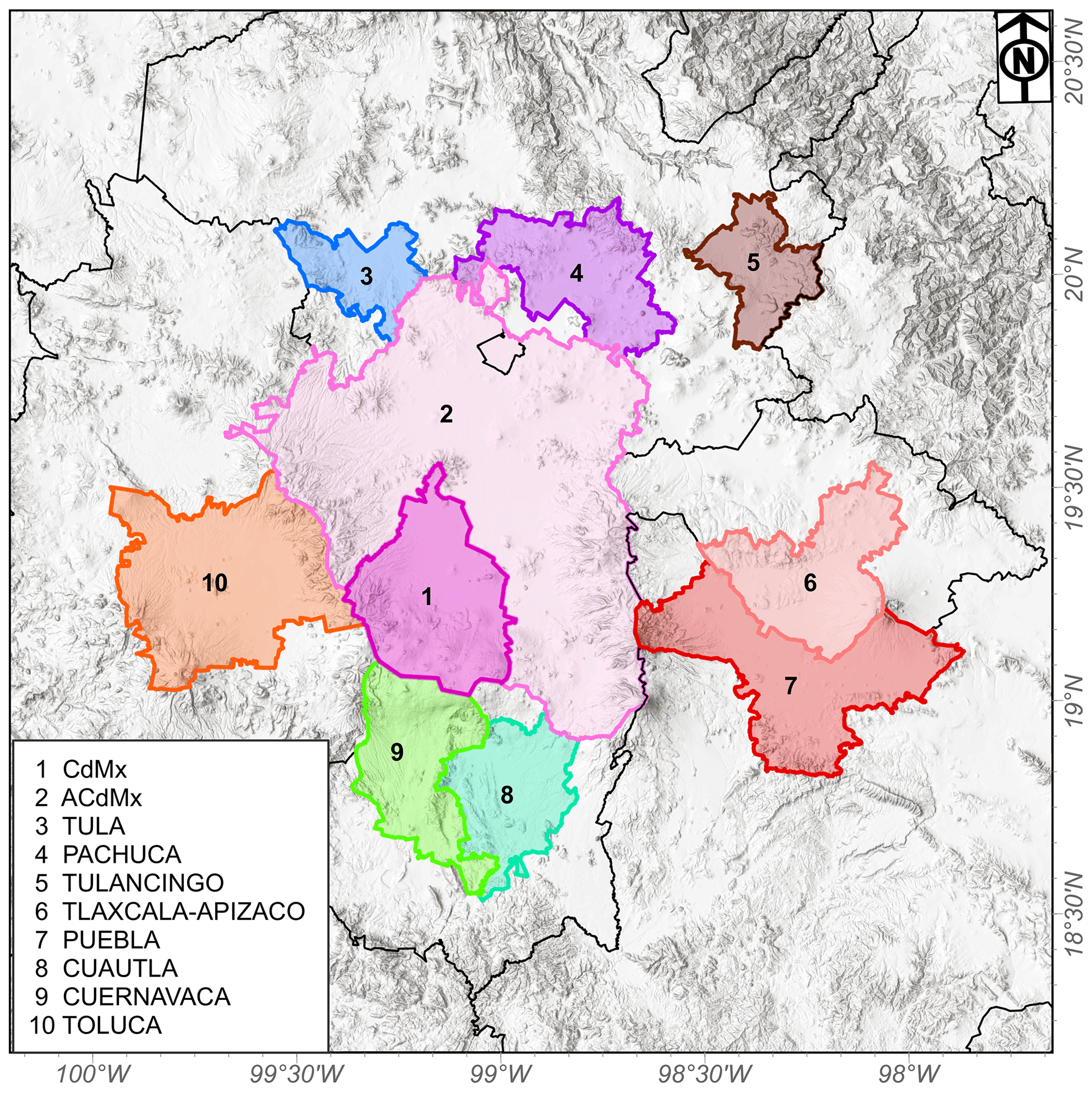
Figure 1Urban districts surrounding Mexico City. For each of the color-coded domains a separate WRF-Chem tracer run was performed based on the emissions within the polygons. The elevation map in the background is under copyright © Esri, Airbus DS, USGS, NGA, NASA, CGIAR, N Robinson, NCEAS, NLS, OS, NMA, Geodatastyrelsen, Rijkswaterstaat, GSA, Geoland, FEMA, Intermap, and the GIS user community.
3.1 The WRF-Chem model
We simulate the TROPOMI CO column concentrations by deploying the WRF-Chem model version 3.9.1.1. The simulation covers the time period of TROPOMI measurements on the regional domain shown in Fig. 1. We ignore photo-chemical oxidation and secondary production of CO in the atmosphere (chem_opt option 106 (RADM2-KPP), as a tracer with gaschem off), which is justified by the long lifetime of CO compared with the size of the model domain as discussed by Dekker et al. (2017). Especially for the region of Mexico City, the contribution of atmospheric chemistry to the total CO concentration is less than 3 % as presented by Mejia (2020). Hence, WRF-Chem simulates the transport of CO surface emissions as traces as done by e.g., Borsdorff et al. (2019) and Dekker et al. (2017, 2019). The spatial resolution of the simulation is chosen to be comparable with the TROPOMI CO product sampling. Each grid cell of the considered simulation domain (270×270 km2) is 3×3 km2. The WRF-Chem simulation employs the emission inventory Inventario Nacional de Emisiones de Contaminantes Criterio (INEM) for the year 2013 but scaled by a factor of 0.48 to make it applicable to the years 2017 to 2019. Here the scaling factor is based on recent SEDEMA surface measurements (García-Reynoso et al., 2018). The inventory includes diurnal, week-to-week, and monthly variations in the CO emissions, where weekly and daily temporal profiles are derived from traffic counts in Mexico. The inventory is described in more detail by García-Reynoso et al. (2018). Finally, the model run is constrained by National Centers for Environmental Prediction (NCEP) North American Mesoscale (NAM) 12 km analysis wind fields (NCEP, 2015) and yields vertical CO concentration profiles for every latitude and longitude grid cell and every model time step and tracer run.
The WRF-Chem simulation uses 10 independent tracers to estimate the CO emissions of the areas Tula, Pachuca, Tulancingo, Toluca, Cuernavaca, Cuautla, Tlaxcala, Puebla, the metropolitan area of Mexico City CdMx, and the adjoint urban area ACdMx. The total simulated CO field is given by the sum of the simulated CO fields of the tracer. Since no atmospheric chemistry is accounted for, each CO tracer field is linear in terms of the corresponding emissions per district:
where αi is the corresponding scaling factor and ki represents the CO tracer field for the reference emissions (adapted INEM data) for αi=1.
Before using our model to simulate TROPOMI data, we interpolate the model fields to the geolocation and time of the TROPOMI observations. Subsequently, we integrate the model CO profiles to total column densities by applying the total column averaging kernel of the TROPOMI CO retrieval following Eq. (1). We summarize this numerical step in the observation operator 𝒪, which transforms the forward model into
Hence, the operator 𝒪 accounts for the TROPOMI-specific vertical sensitivity, which can change from measurement to measurement and so ensures that the comparison between TROPOMI and WRF-Chem is free of the null space or smoothing error (Rodgers, 2000; Borsdorff et al., 2014). Here, the scaling factors αi are not affected by the operation. In a next step, we transform Eq. (3) to
where and with the corresponding emissions Ei,INEM of the INEM inventory interpolated to the TROPOMI overpass time.
To improve the capability of our forward model to fit TROPOMI observations, we introduce a spatially constant CO background field kbg and an altitude dependence term with corresponding scaling factors αbg and αelv. Here, z is the respective elevation of the TROPOMI CO ground pixels and zref=2240 m is an arbitrary reference altitude set to the elevation of Mexico City:
These two effective model components account for the CO contribution over the Mexico City area originating from outside the model domain such as from fires, power plants, biogenic production, and other cities as well as long-range transport (Borsdorff et al., 2019) and an altitude-dependent linear vertical gradient of the CO columns. Both do not interfere with any localized emission sources. They mitigate shortcomings of the WRF-Chem simulations ignoring CO boundary conditions in the model domain.
Finally, for the interpretation of our CO forward simulations, we make an important assumption. Although the WRF-Chem simulations account for the temporal accumulation of the localized CO emissions over days and weeks, we allocate an emission estimate of the corresponding overpass time to each TROPOMI overpass. Here, we assume that a TROPOMI CO image is dominated by the emissions of the urban districts for the particular observation day, where the temporal accumulation of CO from previous days is partly described by the WRF-Chem simulation due to the corresponding scaling of the inventory and partly mitigated by fitting the nuisance parameters αbg and αelv.
3.2 Inversion methodology
Interpreting a series of n TROPOMI CO images,
at overpass times means estimating the corresponding emissions given by the state vector,
where each element comprises
at the corresponding time ti. Our linear forward model in Eq. (5) describes the measurement vector y by
with the forward-model Jacobian matrix , in short y=Kx. Equation (9) can be inverted by
which is equivalent to the solution of the individual problems yi=Kixi due to the block diagonal form of Eq. (9). Here, the norm of an arbitrary vector p is defined by and Se is the measurement error covariance matrix with the variance of the TROPOMI retrieval error on the diagonal.
Due to measurement noise and forward-model errors, the least-squares inversion of Eq. (10) results in unfavorable error propagation and so requires regularization. Because our problem is linear in the state vector x, regularization can be performed as part of the fitting approach or a posteriori to the least-squares solution, without loss of generality. To regularize the noise propagation, we first derive the temporal mean,
from the unregularized solution in Eq. (10). This modifies our cost function to
In this way, we divided the solution of the original inversion problem (10) into two steps: first we determine the mean emissions from the individual least-squares solutions xest,i, which yields the constrained least-squares problem in Eq. (12) to describe the temporal variability. The side constraint guarantees that measurement information is not used twice. Finally, we add an additional Tikhonov side constraint to Eq. (12) to regularize the error propagation,
with
Here, Γ is an appropriate regularization matrix. For a block diagonal form of Γ analogous to the Jacobian matrix in Eq. (9), namely
the minimization problem (13) decomposes into n problems,
which are only coupled by the external side constraint (14). A closer look at our inversion problem shows that the two constraints have similar effects. The Tikhonov constraint minimizes the variation in the state vector around its mean depending on the regularization parameter λ, whereas the external constraint requires strict conservation of the mean.
Therefore, in practice, we solve the inversion (16) and evaluate the external constraint on the mean afterwards to confirm proper use of the measurement information. Its solution is given by
with the gain matrix
The inversion's averaging kernel relates the “true” state vector xtrue,i to xest,i; namely
with
Ai represents the derivative , where its diagonal elements describe the retrieval sensitivity of a state vector element to its true value. The degree of freedom for signal
indicates the total number of independent pieces of information.
To evaluate the fit quality for each overpass, we consider the fit residuals . Additionally, we evaluate the goodness of the fit described by the reduced chi-squared value,
Here L is the number of observations of a single overpass, yerr,i is the retrieval error, and .
3.3 Estimate of the mean emissions
The first step of the inversion described in the previous section means determining the a priori emissions from a set of TROPOMI data with highest information content using a unregularized least-squares fit, Γ=0. Here, the individual emission estimates may be noisy due to enhanced error propagation in the inversion; however, averaging all inversions reduces noise contribution and so gives a reliable estimate of mean emissions for the different districts. The validity of this approach highly depends on the selected dataset of TROPOMI overpasses. On the one hand, the ensemble should be large enough to estimate mean emissions for the considered time period, but on the other hand it should be strictly filtered for cases where the forward model is in good agreement with the measurement such that a stable inversion of all the emissions is possible. The information content of a single overpass varies and depends on several aspects: (1) the number of useful measurements and their cloud coverage changes between different TROPOMI overpasses. Here, clouds shield the lower troposphere, where atmospheric measurements are particularly sensitive to the surface emissions Ei. (2) The pixel size at the swath edge is about 32 km and so about 5 times larger than at the sub-satellite point. This reduces not only the number of pixels covering a certain area but also the sensitivity of the individual TROPOMI observations. (3) The quality of the forward model depends on the meteorological situation, where we consider model simulations for low wind speeds more reliable. These considerations lead to the criteria of the data filtering to determine the mean emissions for each district. We only select overpasses which meet both filter criteria:
-
TROPOMI observations cover 70 % of the data domain.
-
For all observations the across-track pixel size is <15 km.
The filter criteria reduce the original set of 551 overpasses to 199, which we consider to be sufficient to estimate the overall average emission rate per district, yielding . For this we use the median instead of the mean because of its robustness against outliers. With the same reasoning we define the percentile difference,
to describe scattering in the data, which corresponds to the standard deviation of normally distributed parameters. Finally, we calculate the error in the mean using the percentile difference.
3.4 Final data product
Subsequently, the final data reduction step is performed solving the inversion problem (13). For all overpasses, we choose Γi to be a diagonal matrix with
where the zeros ensure that the elements of the state vector αbg and αelv are not regularized. Obviously, the regularization parameter γk must be well-chosen to optimize the balance between minimum error propagation on the fit parameter and maximum information content inferred from the measurement. If γk is chosen to be too small, the propagation of the TROPOMI measurement noise as well as retrieval biases and forward-model errors dominates the inversion. If γk is chosen to be too large, the estimated state vector reproduces the a priori estimate without appropriate use of the information content of the measurement. For our application, we fix the regularization parameter γk for to constant values such that the scatter of the retrieved emissions stays within predefined boundaries.
Considering the temporal variation in the INEM emissions to be about 40 %, we adjusted the regularization parameter such that the retrieved emissions vary within 60 % of their average. The value 60 % is empirically chosen to balance information content against noise propagation. It puts a moderate constraint on the inversion, ensuring on the one hand a stable inversion and on the other hand a realistic variation in the retrieved emissions around the a priori.
One great advantage of the final retrieval product is that it includes the averaging kernel Ai. This can be used to filter the data with respect to the information provided by the TROPOMI measurements. For the emissions of each tracer, we filter on the individual emissions El, considering averaging-kernel values . This form of data mining optimizes the data use, keeping in mind that TROPOMI overpasses may be appropriate for determining one specific source but not all sources simultaneously. The concept of information-content-based filtering turned out to be very useful and enhances the data exploitation compared to the unregularized least-squares fitting used to determine the mean emission values.

Figure 2Background CO concentration for the domain shown in Fig. 1 estimated by fitting the WRF-Chem simulation to the TROPOMI data. (a) Background CO for individual collocations from 9 November 2017 to 25 August 2019. (b) Monthly mean background CO based on the individual collocations. The error bars are the standard error in the mean, and the light-blue line is the time-invariant a priori used in the fit.
Figure 2 shows the CO background that was fitted as an auxiliary parameter during the inversion described in Sect. 3.2. The concentration and its annual cycle are shown. Here, the biomass burning season between February and June causes the corresponding CO enhancement, whereas lower CO concentrations are observed during the rainy season between June and November. The extremely high CO column values on 15 May 2019 are due to the transport of CO-enriched air from wildfires in the southwest of Mexico into the model domain. Figure 3 shows the CO concentration in the state of Mexico under normal conditions and after the fires, which caused a serious health hazard in Mexico City. These types of fires outside the model domain create an inhomogeneous background CO field over Mexico City, which cannot be described by our forward model. Only fitting a constant background is not sufficient in these extreme cases, and so during the fire season many data cannot be used (we excluded the months May and June 2019).
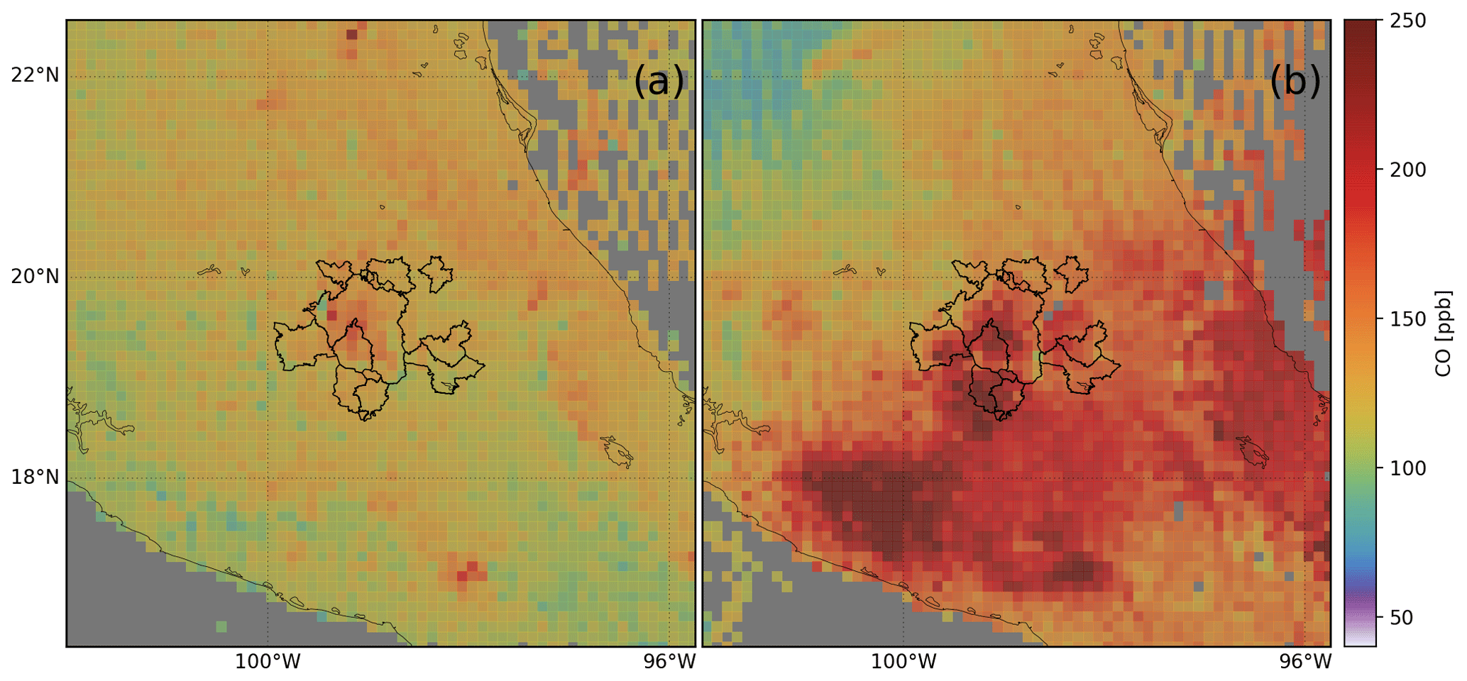
Figure 3TROPOMI CO data over Mexico City averaged on a 0.1 by 0.1∘ lat–long grid. (a) Averaged from 12 to 18 April 2019 showing undisturbed background CO levels. (b) Averaged from 12 to 18 May 2019 showing high CO concentrations in Mexico City caused by fires in the southeast. The street map in the background is under copyright © 2009 ESRI, AND, TANA, ESRI Japan, UNEP-WCMC.
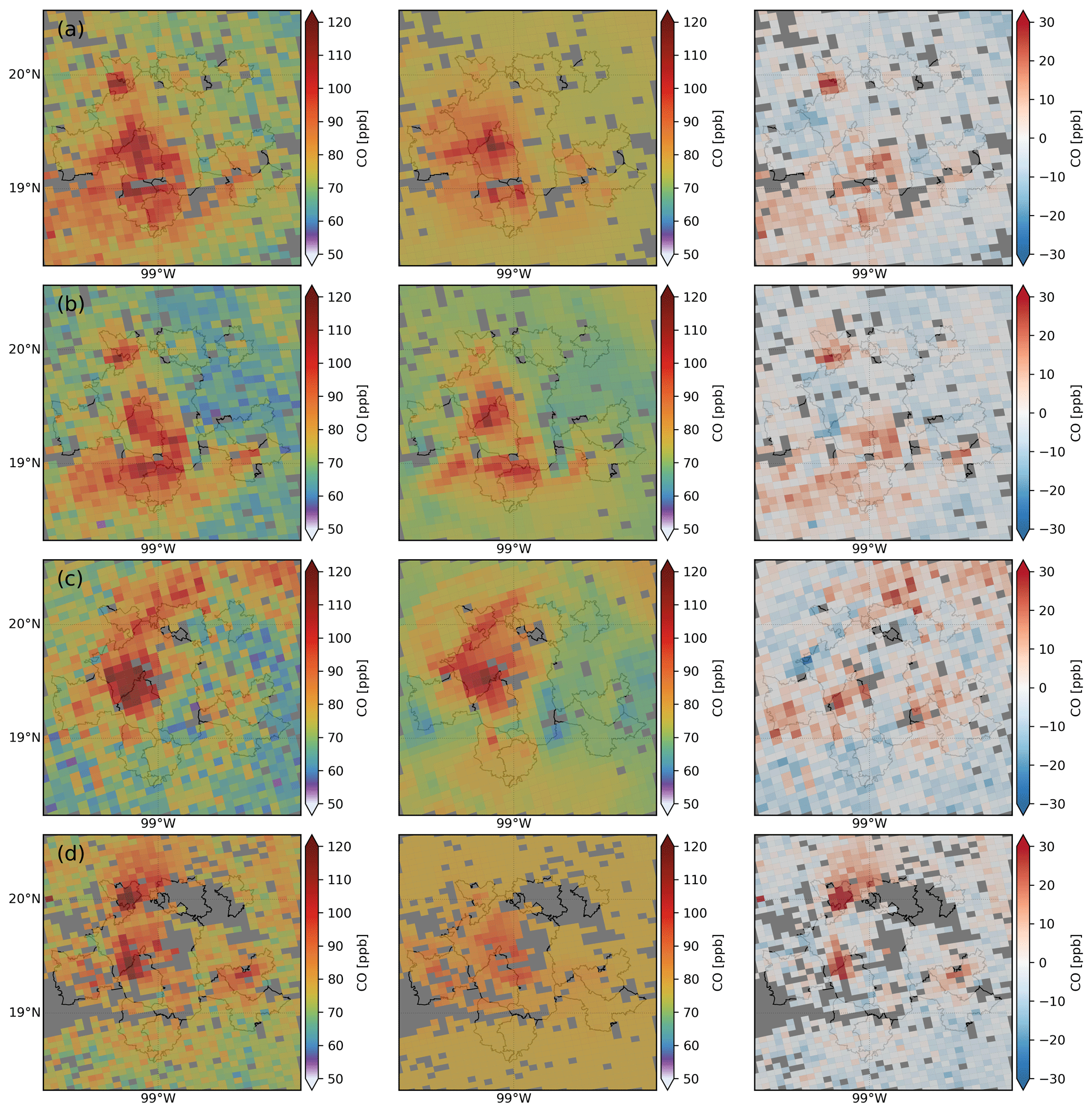
Figure 4Example cases for fitting the WRF-Chem simulation to the TROPOMI data deploying the “final-fit” approach for (a) 20 September, (b) 7 November, (c) 19 November 2018, and (d) 17 August 2019. TROPOMI CO retrievals (left column), WRF-Chem simulation fitted to the TROPOMI data (middle column), and the residual (right column, TROPOMI – WRF-Chem).
Figure 4 shows three examples of TROPOMI overpasses, which include a pixel resolution of 7×7 km2 (panels a, b, and c) and the enhanced spatial resolution of 7×5.6 km2 (panel d), where the latter represents the TROPOMI instrument baseline since 6 August 2019. Focusing on the dry season, the TROPOMI instrument can detect distinct CO enhancements over the different emission areas in central Mexico with the retrievals from single-orbit overpasses (see left column of Fig. 4). After fitting our forward model to the TROPOMI measurements, simulated data and observations are brought into good agreement as illustrated in Fig. 4. Particularly for low-wind-speed conditions in Fig. 4a, TROPOMI and WRF-Chem show distinct CO enhancements over the different emission areas of Mexico. Furthermore, the transport of CO-enhanced air from Mexico City towards the south following the mountain orography and the accumulation of CO in the south is seen by TROPOMI in agreement with the WRF-Chem simulation (Fig. 4c). This clearly shows that regional models like WRF-Chem have a great potential to reproduce the large-scale patterns seen by the TROPOMI instrument. However, we also found clear localized residuals in the difference δj between observations and the forward model (right column of Fig. 4). For atmospheric conditions under high wind speeds the WRF-Chem simulations can deviate more from the TROPOMI measurements as shown in Fig. 4c. Here, the plume of CO-enriched air extending from Mexico City towards the north is simulated as very narrow compared to the more dispersed plume seen by TROPOMI. This points to a possible underestimation of the atmospheric dispersion in the WRF-Chem simulation. A very prominent residual between TROPOMI and WRF-Chem not only is shown in Fig. 4d but also is present in Fig. 4a and b. Here TROPOMI measures a strong CO enhancement in the north of Mexico City that is not reproduced by the WRF-Chem model. This points at a deficient spatial distribution of INEM emissions.
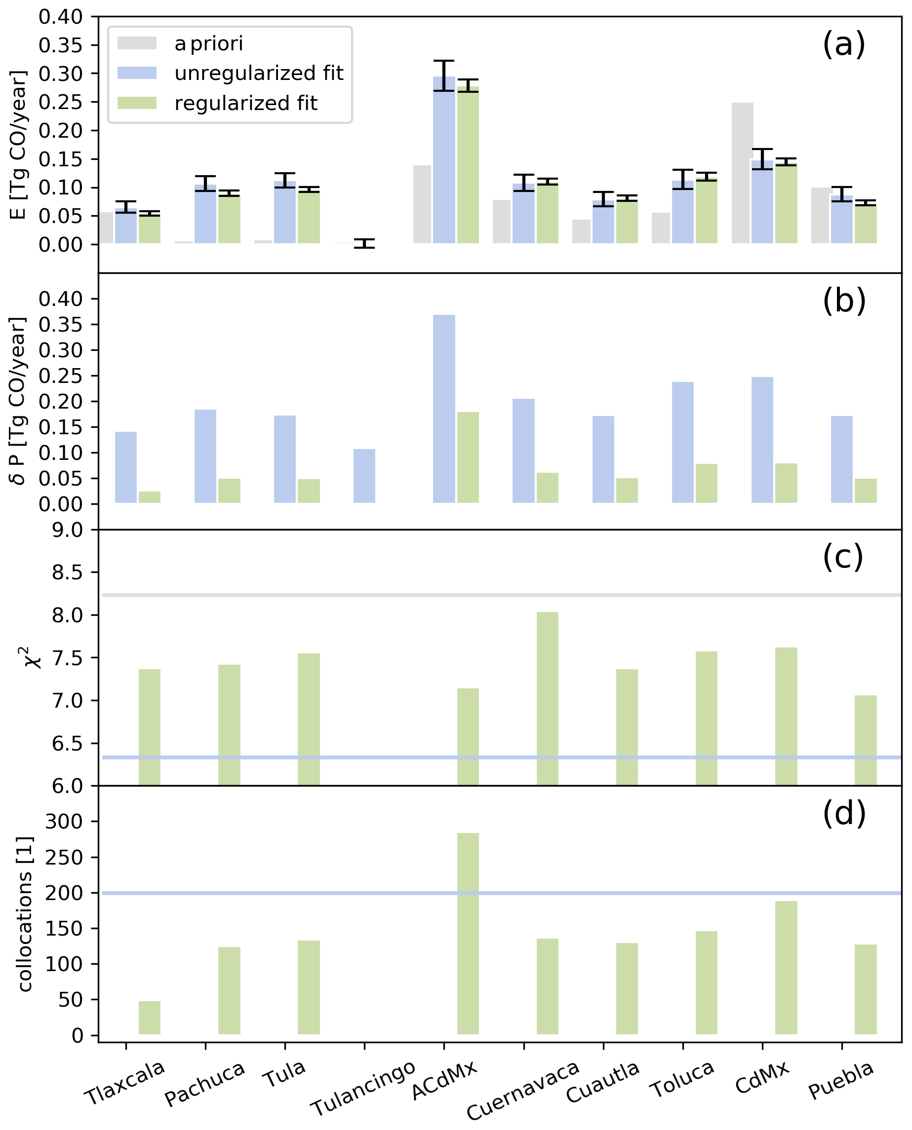
Figure 5Statistics of CO emissions averaged from 9 November 2017 to 25 August 2019 for the tracer domains shown in Fig. 1. (a) Median of the a priori emissions (adapted INEM inventory) used for the WRF-Chem simulation (grey) and retrieved from the TROPOMI data (unregularized fit in blue, regularized fit in green). The error bars indicate the standard error in the mean calculated from the delta percentiles (b) used as a robust estimation of the standard deviation; (c) the median of the goodness of the fit (χ2), and (d) the number of collocations. The number of collocations and the χ2 values of the a priori simulation and unregularized fit are the same for all tracer domains (blue and grey line), but in the final regularized fit they change due to the information content filtering. Here, a collocation corresponds to a specific day because TROPOMI overpasses the region only once.
For each tracer domain Fig. 5a shows the mean emissions of the adapted INEM inventory, the unregularized least-squares fit, and the final data product. The mean emissions agree very well between the last two approaches, indicating that the final inversion in Eq. (17) satisfies the constraint of the predefined mean value. This supports our assumption that the external constraint does not have to be accounted for in the chosen Tikhonov constraint of the inversion. The scatter of the least-squares product is high and in most cases exceeds 100 % (see Fig. 5b), which is expected for the non-constrained inversion. Moreover, we find significant differences between the emissions of the a priori and the final data product. The retrieved emissions for the urban districts Tula (0.10±0.004 Tg yr−1) and Pachuca (0.09±0.005 Tg yr−1) in the north of Mexico City seem to be underestimated by the emission inventory (both were less then 0.008 Tg yr−1). It is not yet clear what sources are missing in the inventory; this needs to be addressed in future studies. However, we identified an oil refinery and a power plant near to Tula and cement and lime kilns near to Pachuca that could have contributed to the CO emissions. Furthermore, we found that the emissions of the central part of Mexico City (CdMx) are assumed to be too high in the adapted INEM inventory (0.25 Tg yr−1), where TROPOMI measurements indicate lower values for CdMx (0.14±0.006 Tg yr−1). This is accompanied by higher values for the adjacent district ACdMx (0.28±0.01 Tg yr−1). The sum of both emissions (0.42±0.016 Tg yr−1) is similar to the a priori emissions (0.39 Tg yr−1). This may mean that the total emissions of the domain including CdMx and ACdMx is well represented in the emission inventory but only the spatial distribution of the source intensity needs refinement.
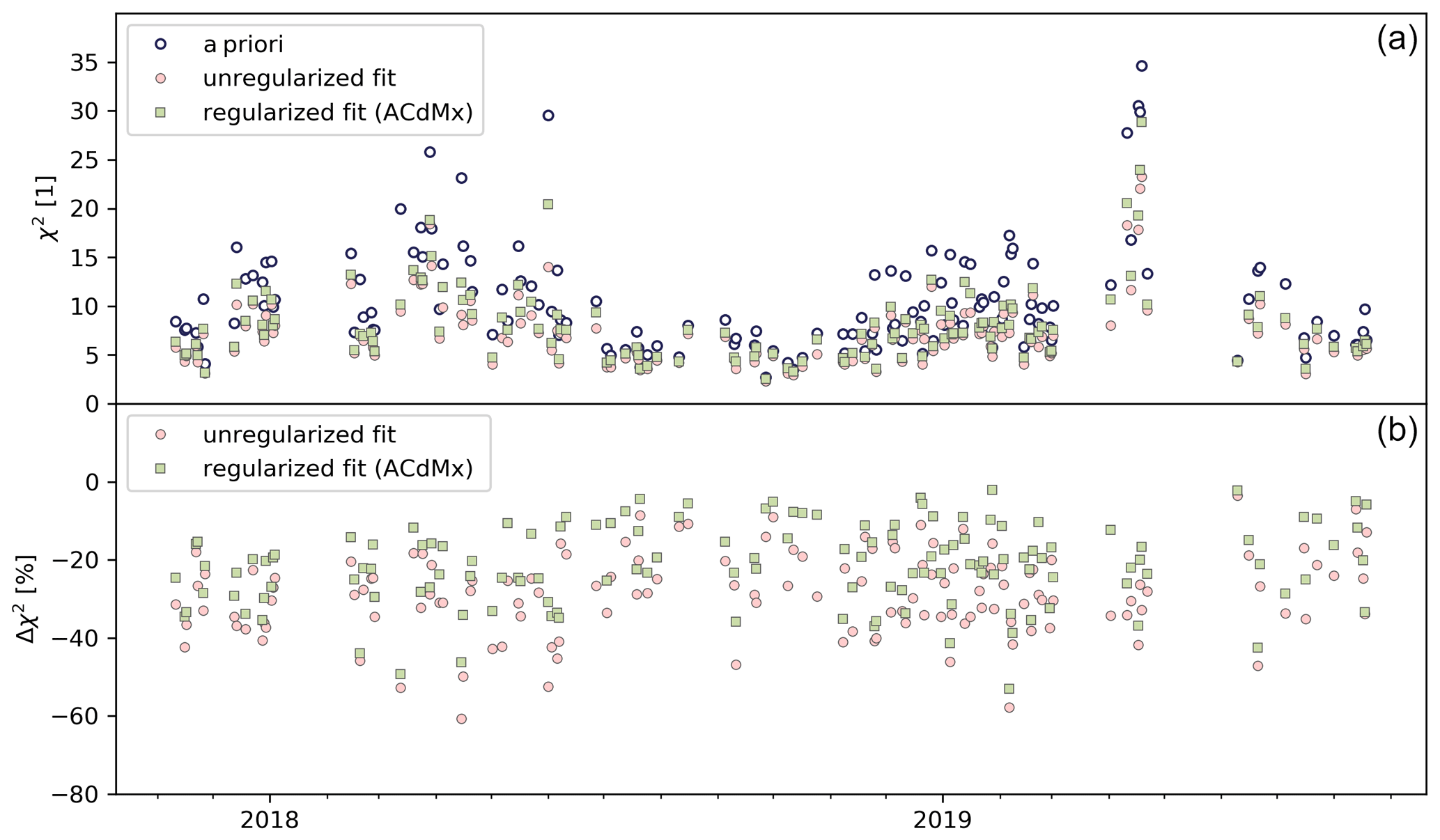
Figure 6(a) The goodness of the fit (χ2) of the TROPOMI CO measurements and the simulation of the WRF-CHEM model for single-orbit overpasses. We distinguish the cases, only fitting background parameters (a priori) and additionally fitting the 10 tracer fields (unregularized and regularized). (b) Improvement of the goodness of the fit (χ2) when fitting the 10 tracer fields (unregularized and regularized) relative to the (a priori) case. For the regularized fit we only show the χ2 of the urban district ACdMx because it provides good data coverage when filtering for the degree of freedom.
The χ2 values in Fig. 5 clearly show that the agreement between TROPOMI and WRF-Chem can be improved by fitting the emissions of the different city districts (blue line) instead of using the INEM inventory (grey line). The regularization approach increases the χ2 values (green bars) because the inversion cannot compensate so well for differences between TROPOMI and WRF-Chem by choosing unrealistic emissions. However, the χ2 values of the final fit are still lower than the ones for the a priori INEM emissions (grey line). Overall, the χ2 values exceeds 1 which indicates that the difference between TROPOMI and WRF-Chem is dominated by systematic errors in the WRF-Chem simulation. Figure 6 shows the χ2 values for the difference between the TROPOMI CO observations of single overpasses and the WRF-Chem simulations over the considered time range of the study. The χ2 values follow a seasonal pattern with enhanced values during the biomass burning season between February and June and low values during the rainy season between June and November. As mentioned before, in the vicinity of other pollution sources (e.g., wildfires) the background variability in CO becomes more complex and can interfere with the retrieved local emissions of Mexico City. Hence, a better model of the CO background concentration and its variability is needed to cope with this effect. However, Fig. 6 also shows that fitting the emissions of the different city districts significantly improves the χ2 between TROPOMI and WRF-Chem over the whole time range and the improvement can be even more than 50 % for single overpasses compared to cases of simulations only using the emission values provided by the INEM inventory.
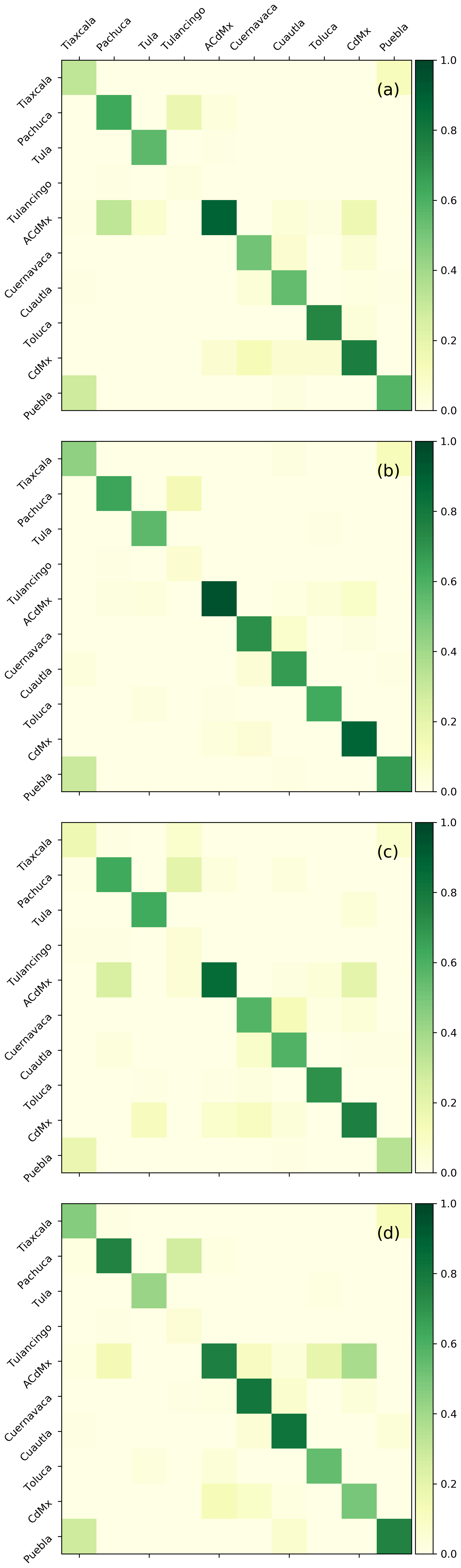
Figure 7Averaging-kernel matrices showing the sensitivity and cross-sensitivities for the scaling of the different tracer fields. The same cases as in Fig. 4 are shown for the dates (a) 20 September, (b) 7 November, (c) 19 November 2018, and (d) 17 August 2019 but deploying the regularized retrieval.
For a correct interpretation of the retrieved emissions the averaging kernel, as shown in Fig. 7 for four example cases, offers several advantages. The figure shows that generally the averaging kernels have high values on the diagonal, indicating high sensitivity to the quantity to be retrieved. It indicates that TROPOMI measurements can be used to distinguish emissions of the different urban districts of Mexico, with the exception of the emissions of the Tulancingo district. Due to the small mean emissions, the averaging kernel indicates a low sensitivity of the data product. Furthermore, the averaging kernel shows cross-correlations between the different elements of the state vector due to the regularization. Although these interdependencies exist, e.g., between the emissions of CdMx and ACdMx as shown in panel (d) of Fig. 7, these are still small compared the diagonal. The averaging-kernel information is very useful to filter the emission product with respect to the information provided by the TROPOMI measurements. Using the sensitivity of individual sources, this results in a different number of coincidences for the different districts (panel c of Fig. 5). This form of data mining optimizes the data use, keeping in mind that TROPOMI overpasses may be appropriate for determining one specific source but not all sources simultaneously. In this manner, error propagation in the inversion can be minimized.
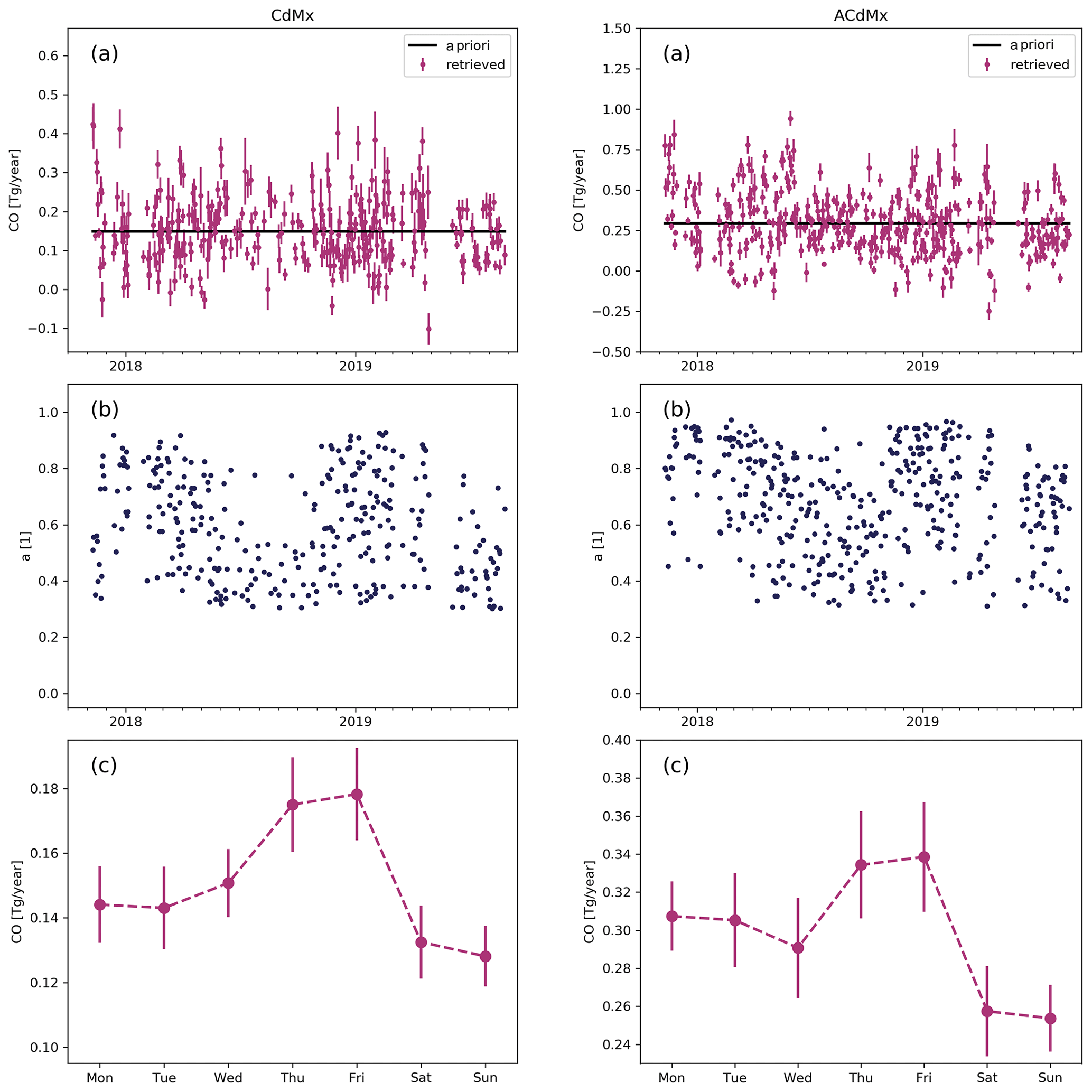
Figure 8Retrieved CO emissions from the TROPOMI data for the tracers CdMx (left column) and ACdMx (right column). (a) Time series of individually retrieved CO emissions. The error bars indicate the error in the fit, and the black line is the time-invariant a priori used in the fit. (b) Degree of freedom of the scaling factor for the tracer field. Only data with degrees of freedom (dofs) >0.3 are accounted for. (c) Weekly cycle of the CO emissions. Median values are shown, and the error bars are the standard error in the mean deploying the delta percentile as a robust estimation of the standard deviation.
Due to the little scatter and the higher number of data of the final data product for the suburbs CdMx and ACdMx, we can draw conclusions about the time-dependent variability in emissions. Figure 8a shows the time series of the emissions for CdMx and ACdMx, which vary around the a priori value. This temporal variation is determined from the measurements as all a priori information is assumed to be time invariant. The scatter of the data is still high and even includes negative values. Even though negative emissions are not physical, we need to keep them in our analyses because filtering negative noise can induce a positive bias in the mean. Panel (b) of the figure shows relatively high values of the diagonal elements of the averaging kernel for the emissions of the two urban districts. Finally, panel (c) of the figure indicates a clear weekly CO cycle in the data with low values during weekends. During the week, the CO emissions of the two districts do not differ significantly due to the error estimates, and more TROPOMI data are required to further constrain the weekly cycle. We found that the CO values on Saturday and Sunday are equally low. An explanation for this could be that the main source of CO in Mexico City during the week is traffic which is responsible for the weekly cycle and the remaining sources of cooking, water heating, etc. should not change much during the weekend.
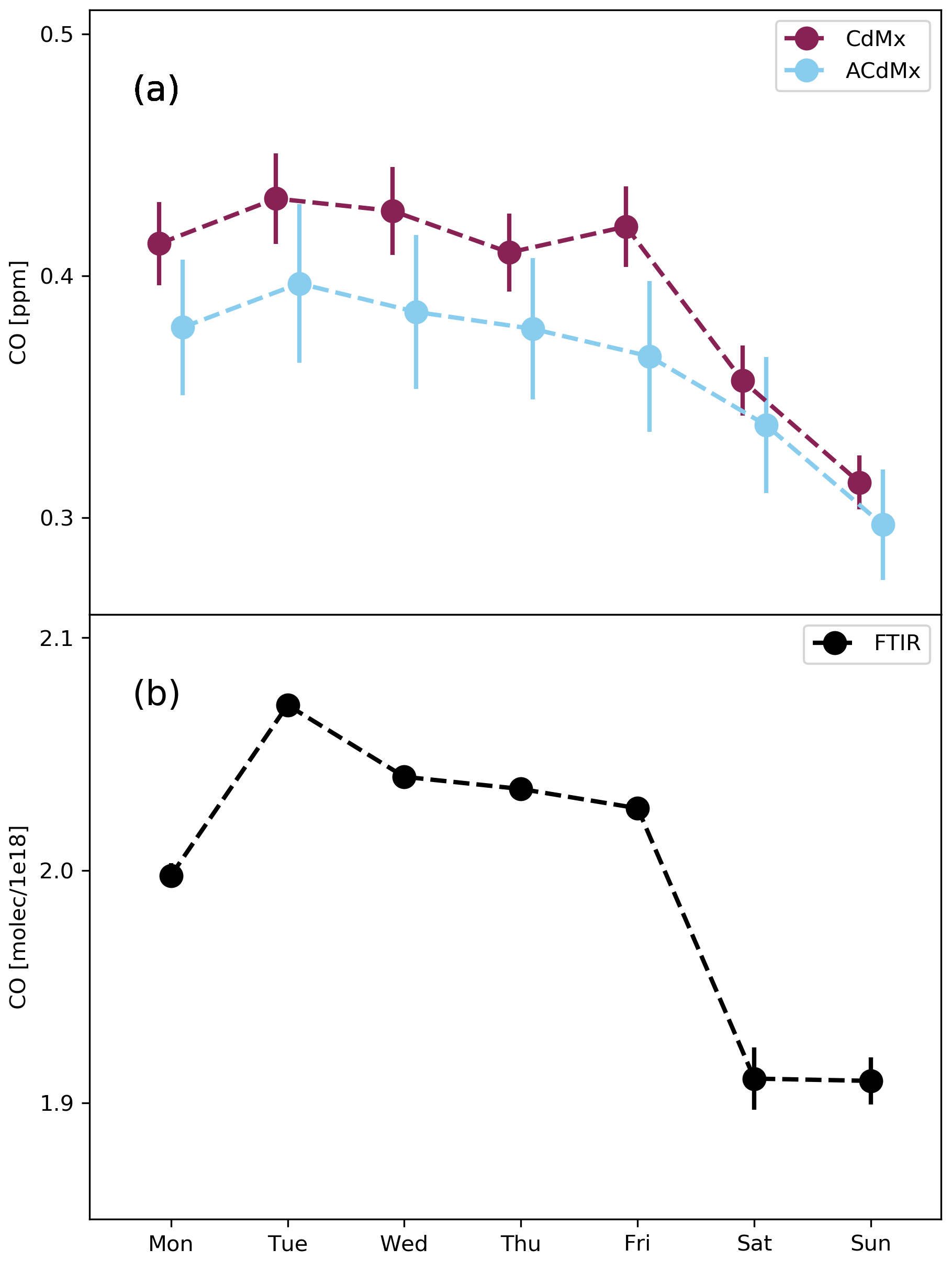
Figure 9Weekly cycle of the CO concentration. (a) Based on 29 in situ measurement station operated by SEDEMA. (b) Ground-based FTIR vertical column measurements of an instrument located in Mexico. Median values are shown, and the error bars are the standard error in the mean deploying the delta percentile as a robust estimation of the standard deviation.
A similar weekly cycle is observed by Mexico City in situ measurements provided by 29 SEDEMA ground stations. For each of the sites, we use data from 2017 to 2018 for the overpass time of TROPOMI (12:00–15:00 local time), calculate a weekly cycle, and group the data into the stations located in the CdMx urban area and those located in the wider area of the metropolis. Figure 9a depicts the median of all weekly cycles and the standard error in the mean with a clear minimum during weekends. The error bars indicate that the overall shape of the weekly cycles for the remaining days varies a lot from station to station.
The lower CO concentrations during the weekend are also detectable with column retrievals from ground-based FTIR measurements in Mexico City, 2280 m a.s.l.; 19.32∘ N, −99.18∘ E, at the campus of the National Autonomous University of Mexico by the Center of Atmospheric Sciences (CCA). The spectra used are recorded in the mid-infrared with a resolution of 0.075 cm−1 (Bezanilla et al., 2014; Plaza-Medina et al., 2017), and the CO column and profile is retrieved using the standard NDACC retrieval strategy (García-Franco et al., 2018; Borsdorff et al., 2018a). Figure 9b shows the averaged weekly cycle with the standard error derived from the column measurements. Due to the low data density at weekends we used the full time range from 5 December 2010 to 10 September 2019 without filtering for the overpass time of TROPOMI. These independent ground-based measurements confirm the weekly CO cycle found in the TROPOMI data. In general, the TROPOMI CO data product agrees very well with retrievals from ground-based FTIR measurements performed by the TCCON network worldwide with an averaged bias of less than 6±3.8 ppb, and the bias with retrievals from NDACC measurements is even lower (Borsdorff et al., 2018a).
In this study, we analyzed TROPOMI CO retrieval from 551 overpasses of the instrument over central Mexico, which corresponds to about 2 years of measurements starting from the 14 November 2017 until the 25 August 2019. We found that urban pollution can be monitored by the TROPOMI CO data. The high signal-to-noise ratio of the measurements allowed us to distinguish distinct CO enhancements over the various urban districts of central Mexico using single-orbit overpasses of TROPOMI with a high spatial resolution of 7×7 km2 that is enhanced to 7×5.6 km2 from 6 August 2019 onwards.
With a dedicated WRF-Chem tracer simulation for the full-time range of the current TROPOMI data record, we could distinguish the contribution of 10 urban districts: Tula, Pachuca, Tulancingo, Toluca, Cuernavaca, Cuautla, Tlaxcala, Puebla, CdMx, and ACdMx. The model data were collocated with the TROPOMI measurements and convolved with the total column averaging kernel to account for the vertical sensitivity of the instrument. Here, the WRF-Chem tracer simulation does not account for atmospheric chemistry, and so the simulated CO tracer fields are linear in the emission rates of the different districts. The model is extended by two effective parameters describing a spatially constant CO background and a dependency of the simulated column on terrain height.
The CO emissions are determined in two steps. First, we apply an unregularized least-squares fit of the model to the TROPOMI observations to determine the averaged emissions per district. A strict data screening based on the measurements and WRF-Chem model simulation reduced the TROPOMI dataset from 551 to 199 overpasses. Second, we solve a regularized least-squares problem, which minimizes the variation in the emissions around their mean to reduce the noise propagation in the inversion. By means of appropriate regularization parameters, we reduce the scatter of the retrieved emissions to about 60 % of the median for all urban districts. For data interpretation and screening, the use of the averaging kernel is of great advantage. The final retrieval product includes an averaging kernel as a retrieval diagnostic, which allows us to analyze retrieval sensitivities and cross-correlations between the inferred emission rates.
The derived averaged emissions for the various urban districts of Mexico deviate significantly from emission estimates of the Inventario Nacional de Emissions de Contaminantes Criterio (INEM) inventory adapted to the period 2017–2019. The TROPOMI emissions from the urban districts Tula (0.10±0.004 Tg yr−1) and Pachuca (0.09±0.005 Tg yr−1) in the north of Mexico City deviate significantly from the INEM inventory with 0.008 Tg yr−1 for both areas. For the emissions of the central part of Mexico City (CdMx), TROPOMI indicates 0.14±0.006 Tg yr−1 versus 0.25 Tg yr−1 INEM emissions, and for the ACdMx district, TROPOMI indicates 0.28±0.01 Tg yr−1 versus 0.14 Tg yr−1 INEM emissions. Together, both districts have similar emissions with 0.42 Tg yr−1 seen by TROPOMI versus 0.39 Tg yr−1 from the inventory, pointing to a different relative distribution of the CO emissions seen by TROPOMI. Moreover, using a posteriori data screening to optimize data selection per emission source allows us to distill a weekly cycle of CO emissions at the districts CdMx and ACdMx from the dataset with a clear minimum during weekends. This finding is in agreement with in situ observations and ground-based FTIR measurement in the metropolis.
Our study shows the need for and the potential of regional atmospheric transport modeling for the interpretation of TROPOMI CO data over metropolitan areas like Mexico City. Here, the CO pollution is a composite of emissions from different districts, and its transport leads to complex CO enhancement patterns in the atmosphere. The WRF-Chem tracer model could simulate the TROPOMI measurements to a great extent; however model errors are still significant and further improvement is required to fully explore the TROPOMI CO observations of urban sources. Another potential error source of our method is the accuracy of the week-to-week and monthly variations in the emissions in the INEM inventory considering the fixed overpass time of TROPOMI. Furthermore, basin cities can be problematic with low wind speed for days, which could lead to the accumulation of signals from more than 1 d in the basins, and this is not yet covered by our approach. To account for this effect in our inversion needs major adjustments, which will be investigated in follow-up studies.
The TROPOMI CO dataset of this study is available for download at ftp://ftp.sron.nl/open-access-data-2/TROPOMI/tropomi/co/ (last access: 16 December 2020, SRON, 2020). The in situ measurements in Mexico City were downloaded from http://www.aire.cdmx.gob.mx (last access: 16 December 2020, UNAM, 2020). The ground-based FTIR measurements in Mexico can be downloaded from http://www.epr.atmosfera.unam.mx/ftir_data/UNAM/CO/VERTEX/v1/ (last access: 16 December 2020, SEDEMA, 2020).
TB and JL performed the TROPOMI CO retrieval and data analysis. AGR, GM, and BMM performed the WRF-Chem simulation. WS and MG provided the ground-based FTIR measurements. All authors discussed the results and commented on the manuscript.
The authors declare that they have no conflict of interest.
The presented work has been performed in the frame of the Sentinel-5 Precursor Validation Team (S5PVT) or Level-1 and Level-2 Product Working Group activities. Results are based on preliminary (not fully calibrated or validated) Sentinel-5 Precursor data that will still change. The results are based on S5P L1B version 1 data.
This article is part of the special issue “TROPOMI on Sentinel-5 Precursor: first year in operation (AMT/ACP inter-journal SI)”. It is not associated with a conference.
The presented material contains modified Copernicus data (2017, 2018). The TROPOMI data processing was carried out on the Dutch National e-Infrastructure with the support of the SURF cooperative. This project was partially supported by the LANCAD-UNAM-DGTIC-179 supercomputer system.
This paper was edited by Hartmut Boesch and reviewed by two anonymous referees.
Bezanilla, A., Krüger, A., Stremme, W., and de la Mora, M. G.: Solar absorption infrared spectroscopic measurements over Mexico City: Methane enhancements, Atmósfera, 27, 173–183, 2014. a
Borsdorff, T., Hasekamp, O. P., Wassmann, A., and Landgraf, J.: Insights into Tikhonov regularization: application to trace gas column retrieval and the efficient calculation of total column averaging kernels, Atmos. Meas. Tech., 7, 523–535, https://doi.org/10.5194/amt-7-523-2014, 2014. a, b
Borsdorff, T., aan de Brugh, J., Hu, H., Hasekamp, O., Sussmann, R., Rettinger, M., Hase, F., Gross, J., Schneider, M., Garcia, O., Stremme, W., Grutter, M., Feist, D. G., Arnold, S. G., De Mazière, M., Kumar Sha, M., Pollard, D. F., Kiel, M., Roehl, C., Wennberg, P. O., Toon, G. C., and Landgraf, J.: Mapping carbon monoxide pollution from space down to city scales with daily global coverage, Atmos. Meas. Tech., 11, 5507–5518, https://doi.org/10.5194/amt-11-5507-2018, 2018a. a, b, c, d
Borsdorff, T., de Brugh, J. A., Hu, H., Aben, I., Hasekamp, O., and Landgraf, J.: Measuring Carbon Monoxide With TROPOMI: First Results and a Comparison With ECMWF‐IFS Analysis Data, Geophys. Res. Lett., 45, 2826–2832, https://doi.org/10.1002/2018GL077045, 2018b. a
Borsdorff, T., aan de Brugh, J., Pandey, S., Hasekamp, O., Aben, I., Houweling, S., and Landgraf, J.: Carbon monoxide air pollution on sub-city scales and along arterial roads detected by the Tropospheric Monitoring Instrument, Atmos. Chem. Phys., 19, 3579–3588, https://doi.org/10.5194/acp-19-3579-2019, 2019. a, b, c, d, e, f
Dekker, I. N., Houweling, S., Aben, I., Röckmann, T., Krol, M., Martínez-Alonso, S., Deeter, M. N., and Worden, H. M.: Quantification of CO emissions from the city of Madrid using MOPITT satellite retrievals and WRF simulations, Atmos. Chem. Phys., 17, 14675–14694, https://doi.org/10.5194/acp-17-14675-2017, 2017. a, b
Dekker, I. N., Houweling, S., Pandey, S., Krol, M., Röckmann, T., Borsdorff, T., Landgraf, J., and Aben, I.: What caused the extreme CO concentrations during the 2017 high-pollution episode in India?, Atmos. Chem. Phys., 19, 3433–3445, https://doi.org/10.5194/acp-19-3433-2019, 2019. a
García-Franco, J. L., Stremme, W., Bezanilla, A., Ruiz-Angulo, A., and Grutter, M.: Variability of the Mixed-Layer Height Over Mexico City, Bound.-Lay. Meteoro., 167, 493–507, https://doi.org/10.1007/s10546-018-0334-x, 2018. a
García-Reynoso, J., Mar-Morales, B., and Ruiz-Suárez, L.: MODELO DE DISTRIBUCIÓN ESPACIAL, TEMPORAL Y DE ESPECIACIÓN DEL INVENTARIO DE EMISIONES DE MÉXICO (AÑO BASE 2008) PARA SU USO EN MODELIZACIÓN DE CALIDAD DEL AIRE (DiETE), Revista Internacional de Contaminación Ambiental, 34, 635–649, https://doi.org/10.20937/RICA.2018.34.04.07, 2018. a, b
Gloudemans, A. M. S., de Laat, A. T. J., Schrijver, H., Aben, I., Meirink, J. F., and van der Werf, G. R.: SCIAMACHY CO over land and oceans: 2003–2007 interannual variability, Atmos. Chem. Phys., 9, 3799–3813, https://doi.org/10.5194/acp-9-3799-2009, 2009. a
Holloway, T., Levy, H., and Kasibhatla, P.: Global distribution of carbon monoxide, J. Geophys. Res.-Atmos., 105, 12123–12147, https://doi.org/10.1029/1999jd901173, 2000. a
Krol, M., Houweling, S., Bregman, B., van den Broek, M., Segers, A., van Velthoven, P., Peters, W., Dentener, F., and Bergamaschi, P.: The two-way nested global chemistry-transport zoom model TM5: algorithm and applications, Atmos. Chem. Phys., 5, 417–432, https://doi.org/10.5194/acp-5-417-2005, 2005. a
Landgraf, J., aan de Brugh, J., Borsdorff, T., Houweling, S., and O., H.: Algorithm Theoretical Baseline Document for Sentinel-5 Precursor: Carbon Monoxide Total Column Retrieval, Atbd, SRON, Sorbonnelaan 2, 3584 CA Utrecht, the Netherlands, 2016a. a
Landgraf, J., aan de Brugh, J., Scheepmaker, R., Borsdorff, T., Hu, H., Houweling, S., Butz, A., Aben, I., and Hasekamp, O.: Carbon monoxide total column retrievals from TROPOMI shortwave infrared measurements, Atmos. Meas. Tech., 9, 4955–4975, https://doi.org/10.5194/amt-9-4955-2016, 2016b. a
Mejia, J. F.: Running WRF in an Atmospheric Modeling Class: challenges and learning experiences, Atmosfera, 2020. a
NCEP: NCEP North American Mesoscale (NAM) 12 km Analysis, https://doi.org/10.5065/G4RC-1N91, 2015. a
Plaza-Medina, E. F., Stremme, W., Bezanilla, A., Grutter, M., Schneider, M., Hase, F., and Blumenstock, T.: Ground-based remote sensing of O3 by high- and medium-resolution FTIR spectrometers over the Mexico City basin, Atmos. Meas. Tech., 10, 2703–2725, https://doi.org/10.5194/amt-10-2703-2017, 2017. a
Pommier, M., McLinden, C. A., and Deeter, M.: Relative changes in CO emissions over megacities based on observations from space, Geophys. Res. Lett., 40, 3766–3771, https://doi.org/10.1002/grl.50704, 2013. a
Rodgers, C. D.: Inverse methods for atmospheric sounding: theory and practice, vol. 2 of Series on atmospheric, oceanic and planetary physics, World Scientific, Singapore, River Edge, NJ, reprinted: 2004, 2008, 2000. a
Schneising, O., Buchwitz, M., Reuter, M., Bovensmann, H., and Burrows, J. P.: Severe Californian wildfires in November 2018 observed from space: the carbon monoxide perspective, Atmos. Chem. Phys., 20, 3317–3332, https://doi.org/10.5194/acp-20-3317-2020, 2020. a
SEDEMA: In situ CO measurements, available at: http://www.aire.cdmx.gob.mx/default.php?opc=%27aKBhnmI=%27&opcion=Zg==, last access: 16 December 2020. a
SMA-GDF: Inventario de Emisiones de la Ciudad de México 2016., Tech. rep., Secretaría del Medio Ambiente de la Ciudad de México: Dirección General de Gestión de la Calidad del Aire, Ciudad de México, 2018. a
Spivakovsky, C. M., Logan, J. A., Montzka, S. A., Balkanski, Y. J., Foreman-Fowler, M., Jones, D. B. A., Horowitz, L. W., Fusco, A. C., Brenninkmeijer, C. A. M., Prather, M. J., Wofsy, S. C., and McElroy, M. B.: Three-dimensional climatological distribution of tropospheric OH: Update and evaluation, J. Geophys. Res.-Atmos., 105, 8931–8980, https://doi.org/10.1029/1999jd901006, 2000. a
SRON: Scientific TROPOMI CO, available at: ftp://ftp.sron.nl/open-access-data-2/TROPOMI/tropomi/co/, last access: 16 December 2020. a
Stremme, W., Grutter, M., Rivera, C., Bezanilla, A., Garcia, A. R., Ortega, I., George, M., Clerbaux, C., Coheur, P.-F., Hurtmans, D., Hannigan, J. W., and Coffey, M. T.: Top-down estimation of carbon monoxide emissions from the Mexico Megacity based on FTIR measurements from ground and space, Atmos. Chem. Phys., 13, 1357–1376, https://doi.org/10.5194/acp-13-1357-2013, 2013. a
UNAM: VERTEX CO retrievals, available at: http://www.epr.atmosfera.unam.mx/ftir_data/UNAM/CO/VERTEX/v1/, last access: 16 December 2020. a
Varon, D. J., Jacob, D. J., McKeever, J., Jervis, D., Durak, B. O. A., Xia, Y., and Huang, Y.: Quantifying methane point sources from fine-scale satellite observations of atmospheric methane plumes, Atmos. Meas. Tech., 11, 5673–5686, https://doi.org/10.5194/amt-11-5673-2018, 2018. a
Veefkind, J., Aben, I., McMullan, K., Förster, H., de Vries, J., Otter, G., Claas, J., Eskes, H., de Haan, J., Kleipool, Q., van Weele, M., Hasekamp, O., Hoogeveen, R., Landgraf, J., Snel, R., Tol, P., Ingmann, P., Voors, R., Kruizinga, B., Vink, R., Visser, H., and Levelt, P.: TROPOMI on the ESA Sentinel-5 Precursor: A GMES mission for global observations of the atmospheric composition for climate, air quality and ozone layer applications, Remote Sens. Environ., 120, 70–83, https://doi.org/10.1016/j.rse.2011.09.027, 2012. a