the Creative Commons Attribution 4.0 License.
the Creative Commons Attribution 4.0 License.
 | 10 Dec 2020
Optical characterization of pure pollen types using a multi-wavelength Raman polarization lidar
Elina Giannakaki
Stephanie Bohlmann
Maria Filioglou
Annika Saarto
Antti Ruuskanen
Ari Leskinen
Sami Romakkaniemi
Mika Komppula
We present a novel algorithm for characterizing the optical properties of pure pollen particles, based on the depolarization ratio values obtained in lidar measurements. The algorithm was first tested and validated through a simulator and then applied to the lidar observations during a 4-month pollen campaign from May to August 2016 at the European Aerosol Research Lidar Network (EARLINET) station in Kuopio (62∘44′ N, 27∘33′ E), in Eastern Finland. With a Burkard sampler, 20 types of pollen were observed and identified from concurrent measurements, with birch (Betula), pine (Pinus), spruce (Picea), and nettle (Urtica) pollen being the most abundant, contributing more than 90 % of the total pollen load, regarding number concentrations. Mean values of lidar-derived optical properties in the pollen layer were retrieved for four intense pollination periods (IPPs). Lidar ratios at both 355 and 532 nm ranged from 55 to 70 sr for all pollen types, without significant wavelength dependence. An enhanced depolarization ratio was found when there were pollen grains in the atmosphere, and an even higher depolarization ratio (with mean values of 0.25 or 0.14) was observed with the presence of the more non-spherical spruce or pine pollen. Under the assumption that the backscatter-related Ångström exponent between 355 and 532 nm should be zero for pure pollen, the depolarization ratio of pure pollen particles at 532 nm was assessed, resulting in 0.24±0.01 and 0.36±0.01 for birch and pine pollen, respectively. Pollen optical properties at 1064 and 355 nm were also estimated. The backscatter-related Ångström exponent between 532 and 1064 nm was assessed to be ∼0.8 (∼0.5) for pure birch (pine) pollen; thus the longer wavelength would be a better choice to trace pollen in the air. Pollen depolarization ratios of 0.17 and 0.30 at 355 nm were found for birch and pine pollen, respectively. The depolarization values show a wavelength dependence for pollen. This can be the key parameter for pollen detection and characterization.
- Article
(4562 KB) - Full-text XML
-
Supplement
(1545 KB) - BibTeX
- EndNote


Pollen has various effects on human health and the environment. The number of people suffering from allergies due to pollen inhalation is rising (Schmidt, 2016). Airborne pollen is recognized as one of the major agents of allergy-related diseases such as asthma, rhinitis, and atopic eczema (Bousquet et al., 2008). Pollen is also a biogenic air pollutant which affects both the solar radiation reaching the Earth and cloud optical properties by acting as nuclei for both cloud droplets and ice crystals (Steiner et al., 2015).
Various networks are built to monitor pollen concentrations at ground level using in situ instruments (Giesecke et al., 2010). In 2020, there are more than 1000 active pollen monitoring stations in the world (Buters et al., 2018; https://oteros.shinyapps.io/pollen_map/, last access: 7 April 2020), with the majority based on the Hirst principle (Hirst, 1952). The conventional method of pollen classification is based on pollen morphological characteristics using microscopy (Holt and Bennett, 2014; Weber, 1998). However, it requires complex procedures for complete classification and identification, and the results are not publicly available online. Besides, pollen grains can be agile and change their visual nature before the analysis, e.g. undergo an osmotic shock (Miguel et al., 2006), which leads to errors in pollen characterization. Several studies on the long-distance transport of pollen (Rousseau et al., 2008; Skjøth et al., 2007; Szczepanek et al., 2017) have shown that pollen grains can be lifted up to several kilometres and be dispersed by wind over thousands of kilometres.
An increasing interest in pollen has arisen in the aerosol lidar community (Noh et al., 2013; Sicard et al., 2016). In our previous study (Bohlmann et al., 2019) we showed on the basis of an 11 d birch pollination period that lidar measurements can detect the presence of pollen grains in the atmosphere and that non-spherical pollen grains can generate strong depolarization (we found a mean depolarization ratio of 0.26 for the birch–spruce pollen mixture). Therefore, it is possible to observe airborne pollen grains in the atmosphere using the depolarization ratio in the absence of other depolarizing non-spherical particles (e.g. dust). We have also reported that lidar-derived parameters (e.g. depolarization ratio and Ångström exponent) provide the possibility of identifying different pollen types (e.g. birch and spruce pollen). However, the optical properties of pure pollen are still missing due to the fact that the atmospheric aerosol population is always a mixture of several particle types. For instance, the depolarization ratio of pure pollen is an essential parameter needed to separate pollen backscatter from the background aerosol backscatter. The Ångström exponent and the lidar ratio, which are often used for aerosol typing, are also crucial parameters to be defined for pure pollen particles.
In this study, we present a novel method for characterizing the optical properties of pure pollen particles, based on a 4-month campaign. In Sect. 2, we introduce the pollen campaign and the instruments. In Sect. 3, we present the methodology and describe a novel algorithm to estimate the depolarization ratio value for pure pollen. This algorithm is tested and validated through a simulator. In Sect. 4, we report the results: firstly, the pollen information observed by the Burkard sampler and lidar-retrieved optical properties for the pollen layer are presented. Secondly, the novel algorithm of Sect. 3 is applied to the lidar observations in Sect. 4.3 to retrieve the optical properties for pure pollen. Section 5 is devoted to the summary and conclusion.
The measurement campaign was performed from May to August 2016 at the Kuopio station of the European Aerosol Research Lidar Network (EARLINET) in Vehmasmäki (62∘44′ N, 27∘33′ E; elevation of 190 m above sea level). This rural site is mainly surrounded by forest, located ∼ 18 km from the city centre of Kuopio, in Eastern Finland. Finland provides suitable conditions for the observation of pollen as 78 % of Finland's total area is covered by forests. Airborne Betula spp. (birch) pollen is one of the most recognized aeroallergens in northern European countries and the most important cause of pollen allergy (Sofiev et al., 2015; Yli-Panula et al., 2009). The predominant Betula species include B. pendula and B. pubescens, while B. nana and B. pubescens subsp. czerepanovii can be found in northern parts of the country. As for conifers, Pinus sylvestris and Picea abies are the most prevalent, and P. sylvestris pollen typically causes the highest peaks during the pollen season. P. sylvestris and P. abies are the only naturally growing species of their genera in Finland. Compared to many other European countries, relatively clean background atmospheric conditions in Finland favour pollen detection and further separation of contributions of pollen backscattering from total scattering by using lidars, since there are fewer other particles, particularly dust, which would complicate the analysis.
The Kuopio station is operated by the Finnish Meteorological Institute, and it has been equipped with a ground-based multi-wavelength Raman polarization lidar PollyXT (Engelmann et al., 2016), Doppler lidar, and in situ instruments next to a 318 m tall mast (for the meteorological observations) since autumn 2012 (Hirsikko et al., 2014). PollyXT has three emission wavelengths (355, 532, and 1064 nm) and seven detection channels (including three emitted wavelength channels, three inelastic Raman-shifted wavelength channels (387, 407, and 607 nm), and the cross-polarization channel at 532 nm). PollyXT has an initial spatial resolution of 30 m and a temporal resolution of 30 s. During daytime, the Klett–Fernald method (Fernald, 1984; Klett, 1981) is applied using the elastic signals to retrieve the extinction coefficient, which describes the combined effect of particle absorption and scattering, and the backscatter coefficient, which describes particle backscattering at a 180∘ scattering angle. During night-time, profiles of extinction and backscatter coefficients at 355 and 532 nm can be derived independently using elastic and inelastic Raman-shifted wavelengths (387 and 607 nm), based on the Raman inversion (Ansmann et al., 1992). The ratio of extinction-to-backscatter coefficient is called the lidar ratio (LR), which is considered an important parameter to separate particle types, as it depends on their single scattering albedo and backscatter phase function, thus being a function of size distribution and chemical composition. The cross-polarization and total polarization channels of the PollyXT allow the retrieval of the volume linear depolarization ratio (VDR) and particle linear depolarization ratio (PDR) at 532 nm, which provide information on the shape of the scattering particles. Multi-wavelength measurements (355, 532, and 1064 nm) enable the determination of Ångström exponents between each wavelength pair, which are related to the particle nature, mostly the size. Previous studies show (e.g. Eck et al., 1999) that Ångström exponent values greater than 2 indicate small particles associated with combustion byproducts, whereas Ångström exponent values less than 1 indicate large particles like sea salt and dust.
In addition to the lidar measurements, a Hirst-type Burkard pollen sampler (Hirst, 1952) was placed 4 m above ground level (a.g.l.) next to the lidar instrument. The Burkard sampler enables identification of pollen types and concentration microscopically with a 2 h time resolution. More detailed descriptions of the pollen sampler and PollyXT used during this campaign can be found in Bohlmann et al. (2019) and reference therein.
In this study, we provide a novel method and develop an algorithm to estimate the depolarization ratio value for pure pollen particles. This algorithm is first tested through a simulator (Sect. 3) using the synthetic lidar data and then applied to the real lidar observations (Sect. 4.3). The simulator includes a direct model and an inverse model module (the block diagram is shown in Fig. S1 in the Supplement); similar ones have already been used for forest and aerosol studies (Shang et al., 2018; Shang and Chazette, 2015). Synthetic data are used in this section to present our methodology. We mainly consider two wavelengths: λ1=355 nm and λ2=532 nm. Other wavelength combinations of 532 and 1064 nm will be briefly discussed at the end of Sect. 3.1.
3.1 Direct model – generation of synthetic optical profiles
Two aerosol populations, pollen (depolarizing) and background (non-depolarizing) aerosols, are considered in this simulation. The optical and physical parameters used in the direct calculation are presented in Table 1; these parameters are named “initial values” for the simulation. The values are based on our lidar measurements (Bohlmann et al., 2019) or literature (e.g. Illingworth et al., 2015). The background here refers to non-depolarizing background aerosols (non-pollen particles), which can be polluted continental or biomass burning aerosols. The depolarization ratios of non-pollen particles (δbackground) at both 355 and 532 nm are selected to be 0.03, which is a mean value for pollen-free periods at our measurement site. Bohlmann et al. (2019) shows that the pollen can generate strong depolarization, thus the depolarization ratios of pure pollen particles (δpollen) at 532 nm are selected as 0.35 as the initial value for the simulation in this section. Pollen grains are quite big and thus can be assumed to be wavelength-independent on the backscatter at wavelengths of 355 nm and 532 nm, with the backscatter-related Ångström exponent (Åpollen) of 0. The backscatter-related Ångström exponent of non-pollen particles (Åbackground) between 355 and 532 nm is assumed to be 2, regarding the previous studies over Arctic regions (e.g. Schmeisser et al., 2018; Tomasi et al., 2012). Note that these values can be changed freely for the simulation under two constraints: (i) the depolarization ratio of pollen (depolarizing one) should be higher than the depolarization ratio of background aerosol (non-depolarizing one); and (ii) the values of backscatter-related Ångström exponent for pollen and non-pollen particles should be different. In addition, the conclusion of the simulation section is not dependent on the assumed profile shape or height; and the initial values are not critical for presenting the overall approach.
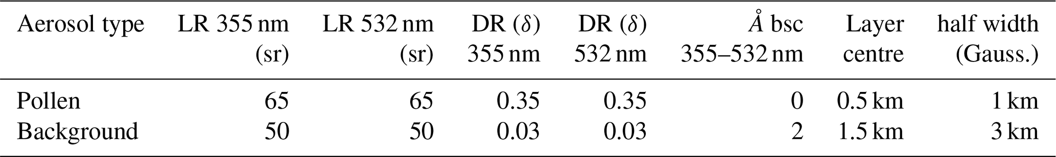
Table 1Parameters of pollen and background aerosol layers as input for the direct model. LR: lidar ratio, DR: depolarization ratio, Å bsc: backscatter-related Ångström exponent. A Gaussian distribution is applied for each layer, with the layer centre and half width given.
The extinction coefficient profiles of these two aerosol layers are assumed to follow a Gaussian distribution. The optical depth (OD) of the input background aerosol layer is fixed to be 0.1 in this simulation. In order to simulate different pollen contributions to the total aerosol load, we change the pollen load by selecting different input values for the pollen layer OD. A pollen OD of 0.002, 0.01, 0.02, 0.05, 0.1, and 1 is used; thus six pollen backscatter coefficient profiles are simulated. One example of simulated pollen and background backscatter coefficients is shown in the Supplement (Fig. S2a) for a pollen OD of 0.1. The pollen layer is defined as the layer below 1 km.
Next, the pollen layer and background layer are summed up (Eq. 1), and then the vertical profiles of aerosol backscatter coefficient, lidar ratio, and Ångström exponent of the total particles are simulated (e.g. Fig. S2b). The Ångström exponent describes the wavelength dependence on aerosol optical properties (Ångström, 1964). The backscatter-related Ångström exponent between two wavelengths of λ1 and λ2 (denoted as Å) can be expressed as Eq. (2).
The index x = pollen, background, or particle denotes the backscatter-related Ångström exponent of pollen, background, or total particles.
Vertical profiles of the particle linear depolarization ratio (PDR; denoted as δparticle) can be also calculated following Eq. (3) (the detailed calculation is given in the Supplement).
Theoretically, these parameters can be derived directly from lidar observations. In order to keep the consistency of the availability of lidar-derived parameters, particle backscatter coefficients at 532 nm, PDRs at 532 nm, and backscatter-related Ångström exponents between 355 and 532 nm simulated for these six cases (shown in Fig. 1) will be used later as input for the inverse model.
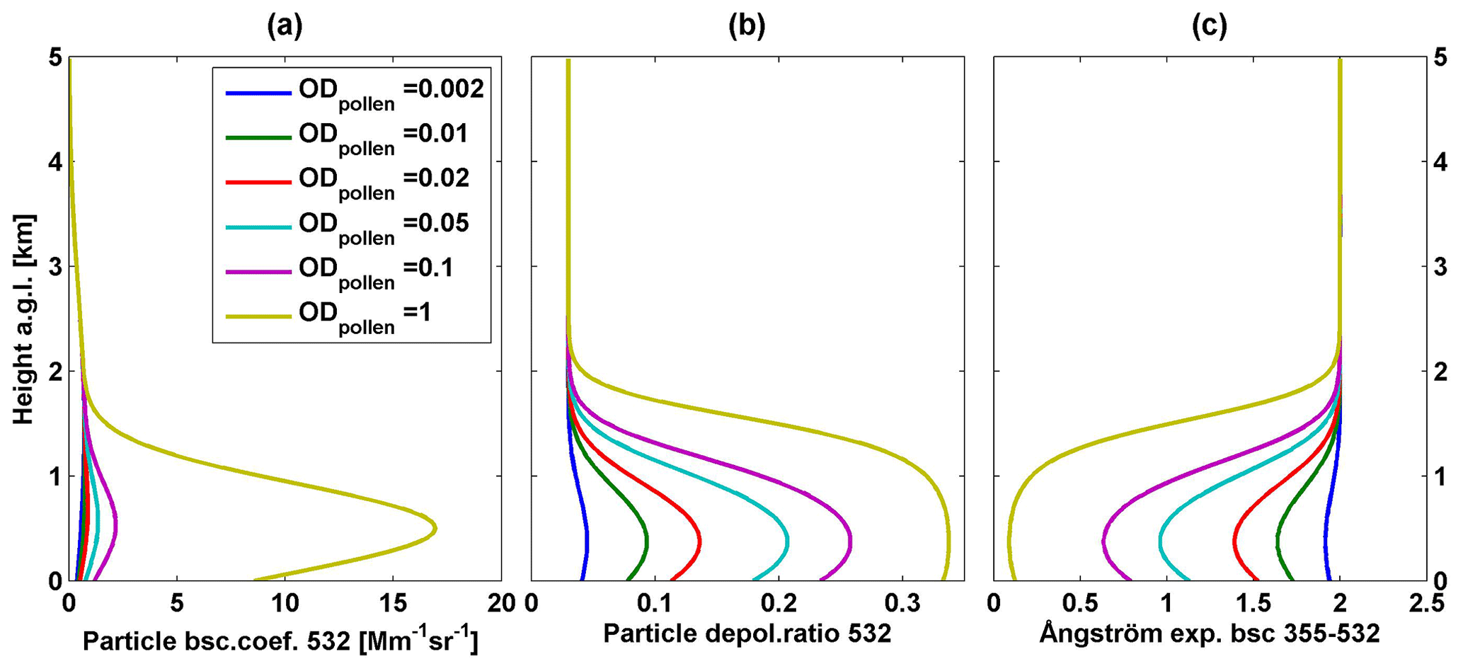
Figure 1Six cases of simulated vertical profiles of (a) particle backscatter coefficient at 532 nm, (b) particle linear depolarization ratio at 532 nm, and (c) backscatter-related Ångström exponent between 355 and 532 nm. Simulated results under different input pollen optical depth (OD) values are shown by colour.
The pollen backscatter contribution, denoted as χpollen (Eq. 4), is defined as the ratio of pollen backscatter coefficient (βpollen) to the total particle backscatter coefficient (βparticle). Note that the use of “particle” here is to distinguish from “molecular”.
We investigate here the relationship of the backscatter-related Ångström exponent of total particles (Åparticle) and pollen backscatter contribution (χpollen) at different wavelengths (the detailed calculation is given in the Supplement), resulting a power law relationship:
The wavelength pairs (λ1,λ2) are selected as (355,532), (532,355), or (1064,532) in this study. In order to simplify the calculation, we introduce two parameters, η and η′, as a function of the backscatter-related Ångström exponent between 355 and 532 nm or between 532 and 1064 nm, for the total particle backscatter coefficients:
The linear relationships resulting from the pairs of parameters η or η′ and χpollen at different wavelengths are reported in Table 2. For example, the pollen backscatter contribution at 532 nm (χpollen(532)) is inversely proportional to the parameter η. Using the previous six simulated cases, a perfect linear relationship is found to fit the η versus χpollen(532) (Fig. 2).
Table 2The linear relationships resulting from the pairs of parameters η(Åparticle) and χpollen at different wavelengths are reported.
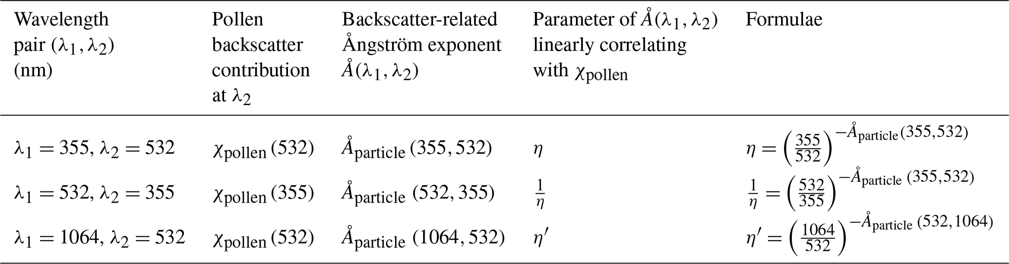
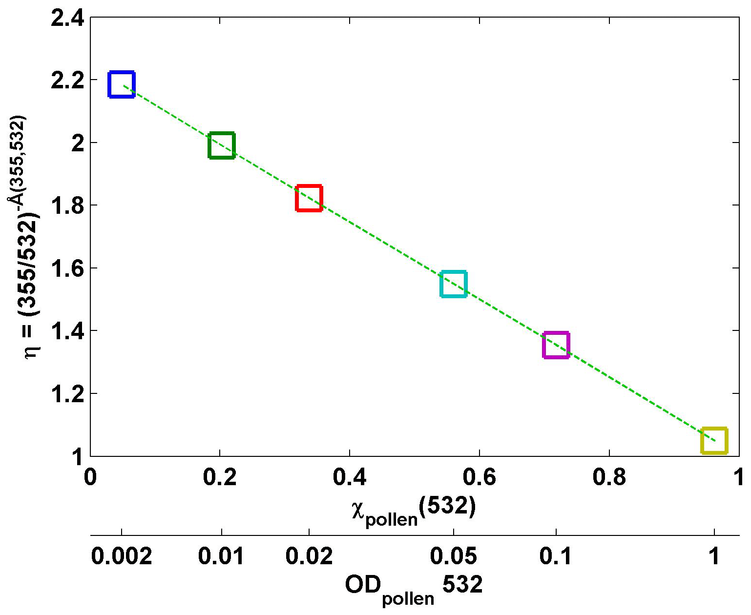
Figure 2Scatter plot using the parameter and pollen backscatter contribution (χpollen) at 532 nm for six simulated cases, of which the input values of pollen optical depth (ODpollen) at 532 nm are defined as 0.002, 0.01, 0.02, 0.05, 0.1, and 1 (shown on the bottom x axis), and the input value of background optical depth is fixed to be 0.1. Mean values of pollen layers (0–1 km) are used for χpollen and η. They line up perfectly following Eq. (5).
3.2 Inverse model – retrieval of depolarization ratio
In this section, we present the inverse model to retrieve the depolarization ratio of pure pollen particles. Tesche et al. (2009) provide a method to separate dust and non-dust contributions, based on the difference of the depolarization ratio values of these two types. This separation method is applied here to separate the two simulated aerosol types.
The pollen backscatter coefficient can be separated from the total particle backscatter coefficient (calculated from Eq. 3), expressed as
The only remaining unknown to solve the Eq. (7) is the depolarization ratio for pure pollen (δpollen). Next we use previously simulated βparticle and δparticle and the assumed δbackground. From now on, 532 nm will be the default wavelength (if not otherwise specified). The wavelength pair (λ1,λ2) is selected as (355,532) in this section. Mean values of optical properties inside the pollen layer are considered in this study; it is also possible to use values of each bin of the synthetic profile which will lead to the same conclusion. Mean values of backscatter-related Ångström exponent between 355 and 532 nm inside the pollen layer, denoted as Å(355,532), can be easily retrieved.
Mathematically, the depolarization ratio for pure pollen can be calculated using Eqs. (4), (5), and (7), as other variables are known or can be assumed. Nevertheless, we developed a retrieval method for this inverse model, so that it can be more easily applied to the real lidar measurements, especially for investigating the depolarization ratio with different values of the unknown Åpollen. An iterate approach is used. In the first step, the depolarization ratio for pure pollen was assumed to be several different values (within the range between 0.03 and 1), denoted as δx, in the simulator. The related pollen backscatter contribution (χpollen(532)) inside the pollen layer can be retrieved using Eqs. (4) and (7). As its value depends on the assumed pollen depolarization ratio (δx), it can be expressed as χpollen(δx,532).
The relationship of Å(355,532) and χpollen(δx,532) was investigated using the parameter η (Eqs. 5 and 6). Examples of scatter plots using mean values of η and χpollen(δx,532) in the pollen layer for cases under the assumptions of δx=0.1, 0.2, 0.3, 0.4 and 0.5 are shown in Fig. 3. For these relationships, perfect linear fits (linear regression relationship) can be found and plotted as dotted lines in Fig. 3, following the simplified equation from Eqs. (5) and (6):
The fitting coefficient (a1,a0) values to determine the estimated parameter η are defined as in Eq. (5). Until this step of the inverse model, no assumption on the Åpollen was made; thus a1 varies for different assumed values of δx. But a0 is constant as the Åbackground is known. Theoretically, for each linear fit equation, χpollen(δx,532) values can range from 0 to 1, with 0 meaning no pollen and 1 meaning 100 % pollen in the observed aerosol particle population. Therefore, for each assumed δx, the η value for can be defined as the value for pure pollen and denoted as ηpure(δx,532).
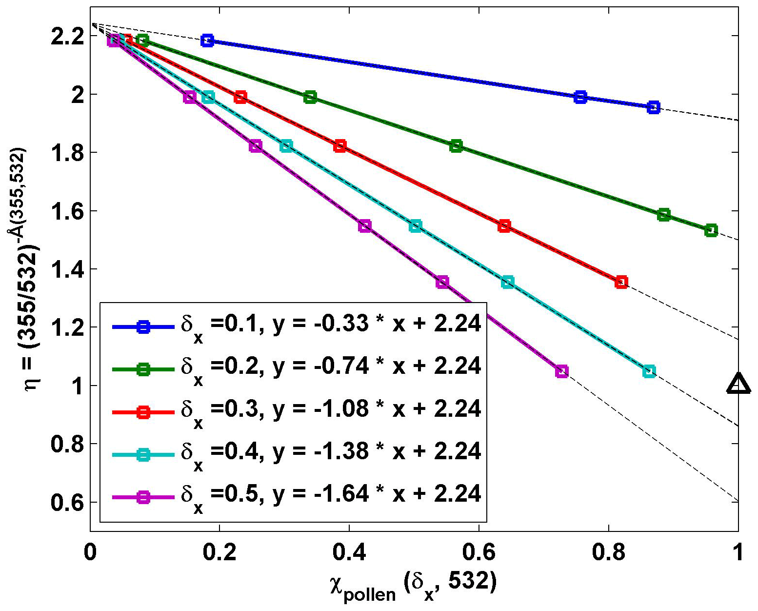
Figure 3Scatter plots of mean values of η and χpollen(δx,532) in the pollen layer in five cases with assumed δx values. η is a parameter using the backscatter-related Ångström exponent between 355 and 532 nm (Eq. 6), and χpollen(δx,532) is the pollen backscatter contribution at 532 nm inside the pollen layer under a certain assumed pollen depolarization ratio value (δx is 0.1, 0.2, 0.3, 0.4, or 0.5). Linear regression lines are drawn by black dotted lines, with the fitting equation shown (Eqs. 5 or 8). The black triangle shows the ideal value: when χpollen is 1, η should be 1 (Å=0).
In Sect. 3.1, the initial value of the backscatter-related Ångström exponent of pure pollen (denoted as Åpollen) between 355 and 532 nm is 0, which results in an initial value of 1 for the parameter η. In this simulation, we assumed that the same value () should be retrieved; the goal was thus to find the value of 1 for ηpure. From previous results shown in Fig. 3, we can see that a δx value between 0.3 and 0.4 may result in ηpure=1 (the black triangle in Fig. 3).
Hence, in the second step, more δx values in that range (0.3–0.4) were used in the simulation, and one can retrieve the relative value of ηpure(δx,532) for each case. These values are presented in Fig. 4. The relationship between δx and ηpure(δx,532) is not perfectly linear, but for these data inside the considered range, a good linear fit can be found with high correlation coefficients . As there is noise in real lidar-measured profiles, two or more values of δx may be found as good solutions. However, after we introduce this additional second linear fit, only one solution will be retrieved in the end.
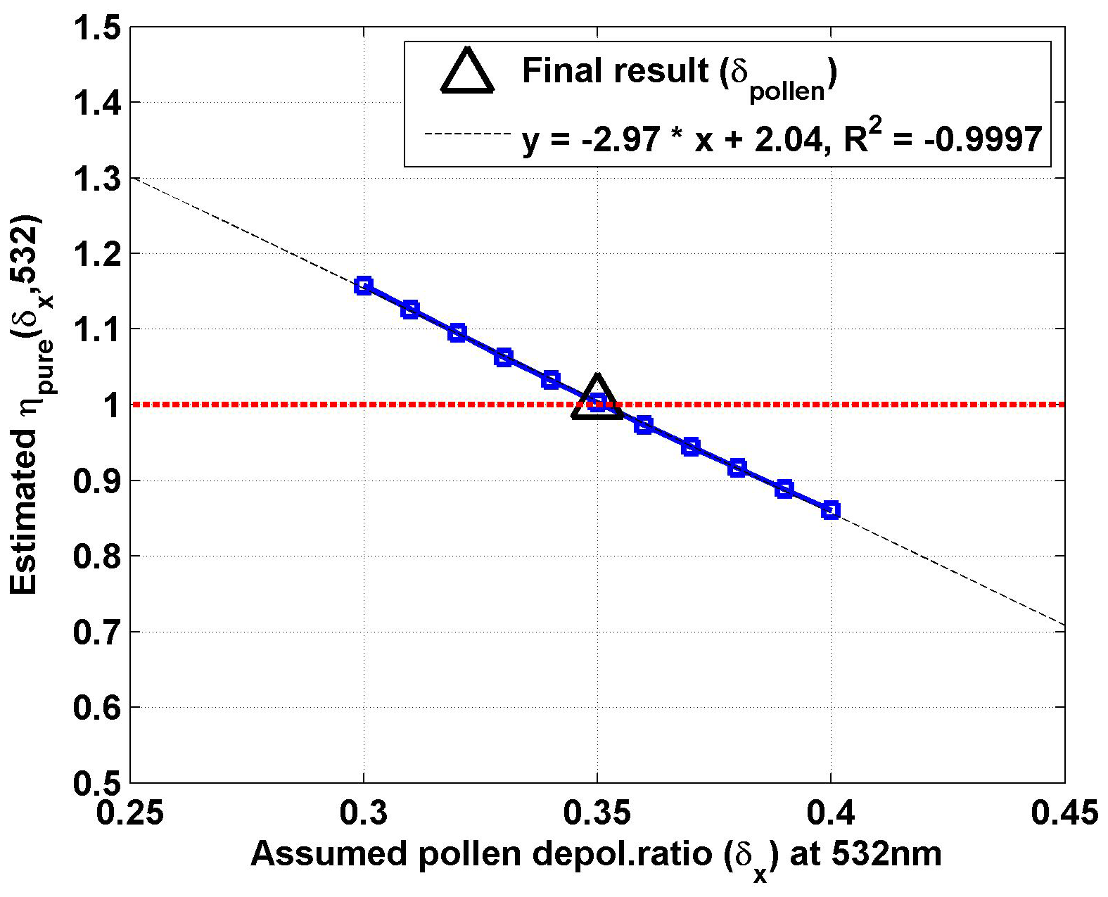
Figure 4Estimated parameter ηpure against the related assumed pollen depolarization ratio δx at 532 nm. ηpure is the η(χpollen) value for the pure pollen (100 % pollen in the observed aerosol particle population, χpollen=1), where η is a parameter using the backscatter-related Ångström exponent between 355 and 532 nm (Eq. 6). The linear regression line is drawn by the black dotted line, with the fitting equation shown. The correlation coefficient (R2) value is also given. The final result of 0.35 for pure pollen is found, resulting in ηpure=1 (i.e. Åpollen=0) (by the black triangle).
Finally, under the assumption of , a pollen depolarization ratio of 0.35 was found, resulting in ηpure=1 (shown by the black triangle in Fig. 4). This result is exactly the same as the initial value of the direct model, which validates the algorithm and provides the feasibility of using this inverse model to retrieve the pure pollen depolarization ratio values. A detailed flow chart of this inverse model is given in Fig. 5. Note that the values of δx can be chosen freely for values bigger than the background depolarization ratio and smaller than 1. This method can also be applied to the other two aerosol types (e.g. dust and non-dust aerosols), under the condition that the depolarization ratio of one aerosol type is the only unknown parameter, and other parameters are known or can be assumed, as long as both the depolarization ratio and the backscatter-related Ångström exponent of the two aerosol types are different.
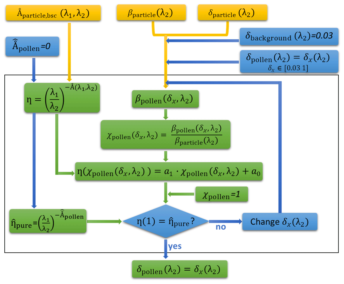
Figure 5Flow chart of the inverse model for the retrieval of the depolarization ratio value for pure pollen. The orange boxes are for the measured parameters (or simulated output from the direct model), the blue boxes for the assumptions/manual input and the green boxes for the estimations/calculations. A detailed description is in Sect. 3.2. The wavelength pair (λ1,λ2) is selected to be (355,532), (532,355), or (1064,532) in this study.
3.3 Uncertainty study
The uncertainty study of this method is investigated in this section. The input parameters (i.e. initial values) of the direct model are defined in Sect. 3.1, with an optical depth (OD) of the background aerosol of 0.1 and pollen OD of 0.002, 0.01, 0.02, 0.05, 0.1, or 1. Nonetheless, some input parameters (e.g. the pollen depolarization ratio δpollen and the backscatter-related Ångström exponent for pollen Åpollen) were selected as different initial values for different uncertainty studies, which are clarified in each paragraph. The output of each direct model simulation was then used as the input for the inverse model.
Under ideal conditions, which means there is no noise on the input profiles for the inverse model, the depolarization ratio of pollen (depolarizing one) can be retrieved perfectly as long as the value is higher than the depolarization ratio of background aerosol (non-depolarizing one). δpollen of 0.04 has been tested, and the correct value was successfully retrieved. Note that for this case, the assumed values of δx should be selected as lower values (e.g. from 0.03). The more values of δx that are used in the inverse model, the better precision will be for the results, but a longer computation time is also needed. It is also possible to combine the first and second steps of the inverse model, by using many assumed values of δx (e.g. 0.032, 0.033, 0.034, …, 0.98, 0.99) for the first step, at the cost of a long computation time.
In the cases presented, we assumed that the backscatter-related Ångström exponent of pure pollen between 355 and 532 nm to be used in the inverse model (denoted as ) is 0, which was the same as the initial value (Åpollen) of the direct model. But in reality, such information is not always available. Under different initial values of Åpollen, there will be a bias on the estimated values of pollen depolarization ratio if the assumed value is different (i.e. ). For example, if the initial value Åpollen is 0.25 (i.e. ηpure=1.11), but we keep the assumption of in the inverse model, the estimated pollen depolarization ratio is found to be 0.39 with a bias of 0.04 (show in Fig. S3). The uncertainty due to the difference between the initial value of Åpollen and assumed was simulated (shown in Fig. S4), where is always assumed to be 0 in the inverse model. For initial values of (i.e. bias of 0.5 on the assumed value of 0), relative uncertainties were assessed to be ∼30 %. This uncertainty due to the difference of initial values of Åpollen and Åbackground was also investigated. The larger the difference between the two values (Åbackground−Åpollen), the smaller the uncertainty. For instance, if we use 3 (instead of 2) as the initial value of Åbackground, the estimated pollen depolarization ratio is 0.37 (instead of 0.39), with a smaller bias for the above example.
Further on, we investigate the random uncertainty due to the noise on input lidar profiles, using the simulator and based on a Monte Carlo approach. The parameters for the six cases simulated earlier (as defined in Sect. 3.1, with values given in Table 1) are used again in this simulation, but noises are additionally added, considering normal statistical distributions, which are introduced by a normal random generator (Fig. S1). The PDR and Å are calculated from particle backscatter coefficients, so we only need to apply different noise levels to the particle backscatter coefficients in the direct model, and related PDR and Å with noise can be retrieved. To simplify the problem, the initial noise levels for both backscatter coefficients at 355 and 532 nm were considered under the same assumptions. We defined “one group” as one draw of six simulated backscatter profiles with a certain noise level; these six backscatter profiles have a pollen OD of 0.002, 0.01, 0.02, 0.05, 0.1, and 1. For each statistical simulation, we used 200 draws (i.e. 200 groups of profiles). This uncertainty study was investigated in two parts:
- i.
Fix the input pollen depolarization ratio, and change the noise levels. We used 0.35 as the initial pollen depolarization ratio. In the case of taking 10 % as the noise level on the backscatter coefficients, one group of six simulated profiles with noise is shown in Fig. 6. A pollen depolarization ratio of 0.354 was found for this group using the inverse model, with a bias of 0.004 compared to the initial value of 0.35. Similarly, pollen depolarization ratio values were retrieved for each of the 200 generated groups. These 200 values had a mean value of 0.351±0.009; thus an uncertainty of 0.009 (relative uncertainty of 2.6 %) was found. We changed the noise levels (e.g. 1 %, 10 %, 20 %, 40 %, and 60 %) on the backscatter coefficients by the normal random generator, and 200 draws were performed for each statistical simulation under each noise level. The uncertainties of the retrieved pollen depolarization ratio against the noise levels were assessed and are shown in Fig. 7a.
- ii.
Fix the noise level, and change the input pollen depolarization ratio. In the second simulation, we keep 10 % as the noise level on the backscatter coefficients, and change the input pollen depolarization ratio values to 0.1, 0.2, 0.3, 0.4, and 0.5. Under each assumption, 200 draws were performed to derive the uncertainty values, which are reported in Fig. 7b. Relative uncertainties on the retrieved pollen depolarization ratio of 1.6 % to 2.8 % were found.
From the simulation results, small uncertainty and a good accuracy were found using this algorithm. Nevertheless, even with the introduced noise levels, these simulations were still performed under quasi-ideal conditions. For each simulated group, six cases were used to provide a wide range of values of χpollen (from ∼0.05 to ∼0.95), which leads to good constraints to find a fitting line for the regression relationship of χpollen and η (Eq. 6) (e.g. Fig. 3). If only three cases (with a pollen OD of 0.01, 0.02, and 0.05) were used for each group, uncertainties 2 to 5 times bigger were found. It is hard to give qualitative values for such an uncertainty study, but the wider range of χpollen values that are in the data set, the better the retrievals will be. The vertical resolution used here was 30 m (as the raw resolution of our lidar); and increasing the vertical resolution of the lidar would result in a smaller uncertainty in the simulation.
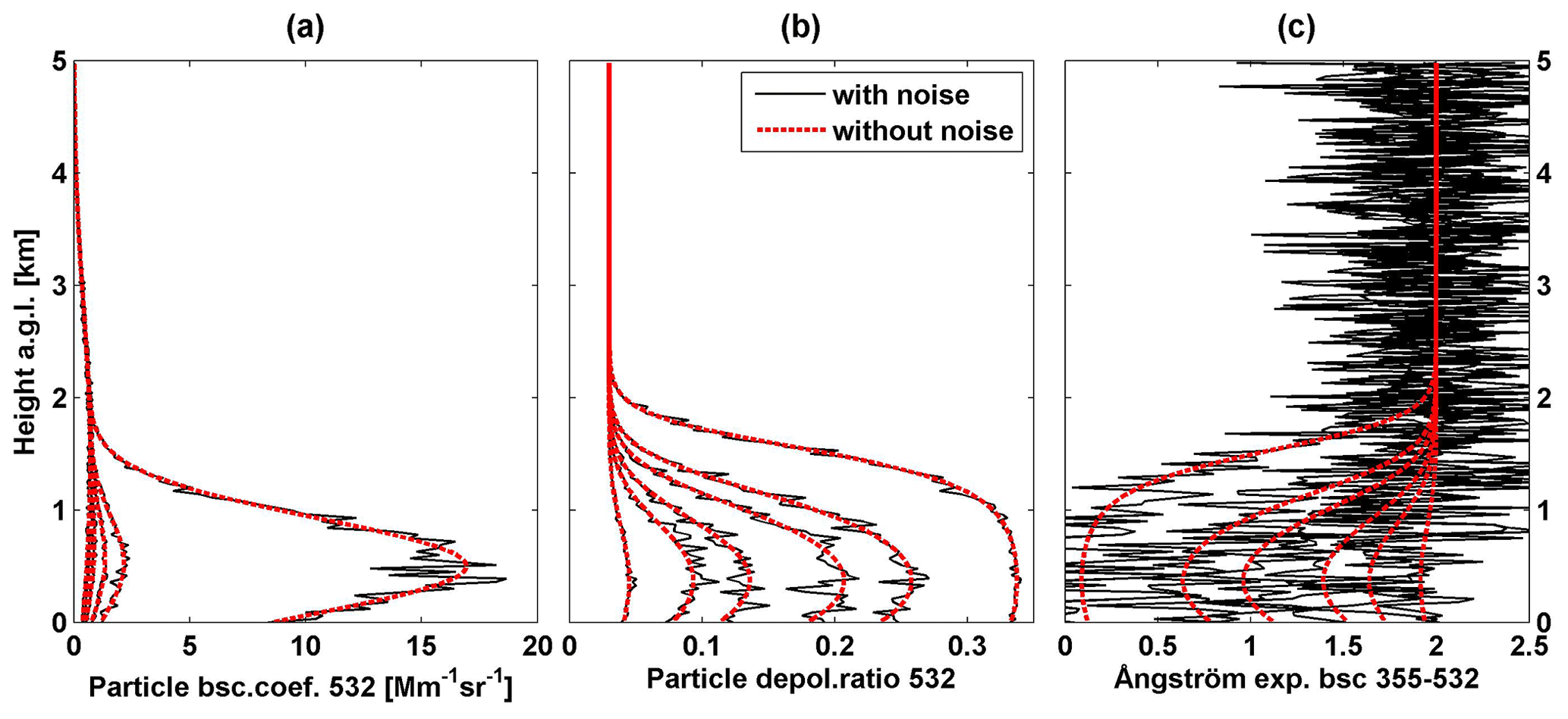
Figure 6Example of one group of six simulated profiles of (a) particle backscatter coefficient at 532 nm, (b) particle linear depolarization ratio at 532 nm, and (c) backscatter-related Ångström exponent between 355 and 532 nm. Profiles without noise are shown by dashed redlines, and ones with noise are shown by black lines. Noise levels on backscatter at both 355 and 532 nm were set to 10 %. Simulated results under six input pollen optical depth (OD) values of 0.002, 0.01, 0.02, 0.05, 0.1, and 1 (same as Fig. 1).
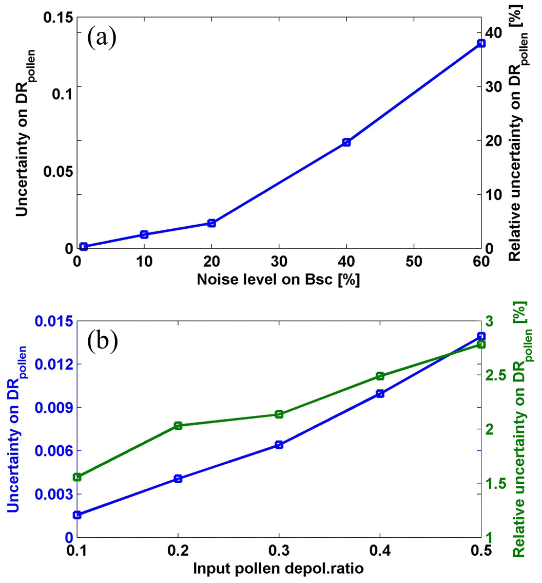
Figure 7Examples of estimated uncertainties (left y axis) and relative uncertainties (right y axis) on retrieved pollen depolarization ratio (DRpollen) at 532 nm against (a) the applied noise levels on backscatter coefficient (Bsc), and (b) the initial input values of DRpollen, using Monte Carlo method. The initial input value of DRpollen is 0.35 for the example in (a). The noise level on backscatter coefficient (Bsc) is 10 % for the example in (b).
4.1 Pollen grain and intense pollination period
During the 4-month campaign, 20 pollen types were observed and identified from the samples collected with the Burkard sampler, six from broadleaved trees, observed from the end of April to mid-June; three from coniferous trees, with a pollination period from mid-May to mid-June; and 11 from grass/weeds, observed mainly in July and August. Among them, birch (Betula), pine (Pinus), spruce (Picea), and nettle (Urtica) pollen were most abundant, contributing to more than 90 % of the total pollen load, regarding number concentrations. The surrounding forest is mixed in terms of the tree species, but the pollination periods of different dominant pollen types are distinct, as can be seen from the Burkard-observed number concentration of specific pollen types shown in Fig. 8a.
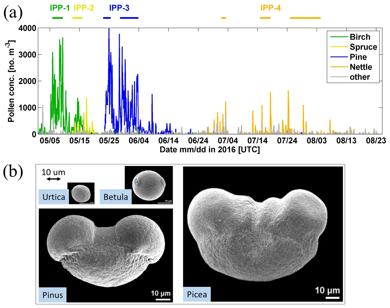
Figure 8(a) Pollen concentration (2 h average) measured by the Burkard sampler at roof level. The main pollen types are shown according to the colour code. Defined intense pollination periods (IPPs) are shown by lines on the top. (b) Microphotographs of pollen grain: Urtica (nettle pollen), Betula pendula (birch pollen), Pinus (pine pollen), Picea abies (spruce pollen). Source: PalDat – a palynological database (https://www.paldat.org, last access: 7 April 2020).
Microphotographs of pollen grains for the dominant pollen types are shown in Fig. 8b (photos taken from https://www.paldat.org, last access: 7 April 2020). Pine and spruce pollen belong to the Pinaceae family, which pollinate profusely and greatly contribute to the pollen counts. However, they are rarely considered as being allergenic. Their pollen grains are large due to their sacs or bladders, which make them easy to identify. Among winged grains, the body is sub-spheroidal to broadly ellipsoidal. The longest axis (sacci included) of Pinus sylvestris (Scots pine) pollen grains is 65–80 µm, while in Picea abies (Norway spruce) the axis is longer, 90–110 µm (Nilsson et al., 1977). Birch pollen can cause severe pollinosis and is recognized as one of the most important allergenic sources (D'Amato et al., 2007). Birch pollen grains are sub-oblate to oblate. B. pubescens pollen grains are 18–24 × 22–28 µm in size (Nilsson et al., 1977), and B. pendula (Silver birch) pollen grains are more or less the same size (personal communication with Sanna Pätsi from Aerobiology, University of Turku, 2020). Nettle is considered moderately allergenic, both in terms of skin tests and amount of exposure to the pollen in the air. Nettle (Urtica dioica) pollen grains are oblate spheroidal to spheroidal and are quite small, with a size of 13–17 × 15–20 µm (Nilsson et al., 1977). Information on the dominant pollen types is reported in Table 3, where the pollen season is defined using the 95 % method (Goldberg et al., 1988). The start of the season was defined as the date when 2.5 % of the seasonal cumulative pollen count was trapped and the end of the season when the cumulative pollen count reached 97.5 %.
Table 3(a) Dominant pollen types with their pollen season period, Latin name (taxa), and typical size. (b) Selected intense pollination periods (IPPs) and the presented dominant pollen types during each IPP. See more descriptions in Sect. 4.1.
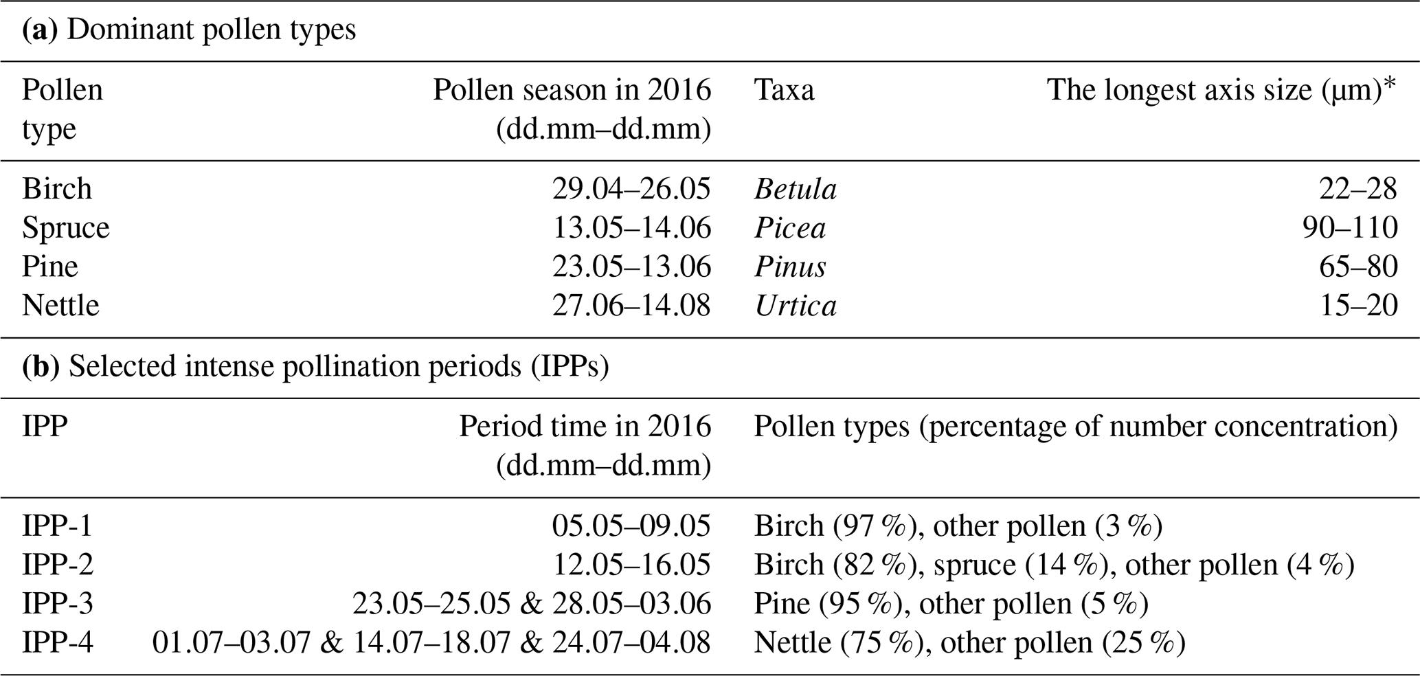
* Values from Nilsson et al. (1977).
Four intense pollination periods (IPPs) are defined considering the pollen seasons and the daily mean pollen concentration values of these four dominant pollen types (Table 3). A minimum value of 300 no. m−3 (for daily mean pollen concentration) was used as the threshold for the determination of IPP-1 and IPP-3, whereas a smaller threshold of 20 no. m−3 was used for IPP-2 and IPP-4. In addition, the availability of lidar measurements was considered for the IPP definition. IPP-1 and -2 are selected within the birch pollen season. During IPP-1, almost only birch pollen is observed (97 % contribution to number concentration), while during IPP-2, spruce pollen is additionally present in the air, with 14 % contribution. IPP-3 consists of two periods within the pine pollen season, separated by a few days with frequent low-level clouds (below 1 km) or rain, causing the relatively low pine pollen concentration between these two periods. IPP-4 is defined for the nettle pollen study for three separate short pollination periods in July and August.
4.2 Optical properties of pollen layer
4.2.1 Pollen layer
A pollen layer in the lidar measurements is defined as the lowest observed layer. The layer boundaries are determined using the gradient method (Bösenberg and Matthias, 2003; Flamant et al., 1997; Mattis et al., 2008) based on the lidar-derived backscatter coefficient profile at 532 nm wavelength. A more detailed description of the layer definition method is described in Bohlmann et al. (2019). In this study, 2 h time-averaged lidar profiles are used to match the pollen sampler time resolution. The retrieved pollen layers are shown in Fig. 9a. With an overlap correction applied in this study, the lower limit for reliable backscatter profiles was about 600 m a.g.l. Statistical values of the pollen layer top height above ground level for the four IPPs were 1.5±0.3, 1.3±0.3, 1.3±0.4, and 1.2±0.3 km, respectively (Fig. 9b). The lowest layer top height was found for the nettle pollen, belonging to herbaceous species. For the relatively larger spruce and pine pollen, the layer top heights were lower compared to the smaller birch pollen.
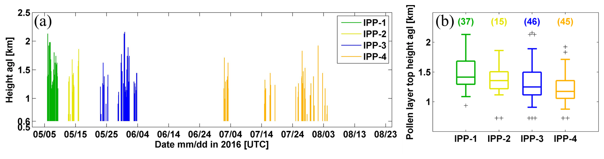
Figure 9(a) Pollen layer definition for four intense pollination periods (IPPs). (b) Box plot of pollen layer top heights during each IPP. The number of available profiles is given. Colours are related to the IPPs.
4.2.2 Lidar-derived optical properties
Mean values of lidar-derived optical properties inside the detected pollen layers were retrieved (Table 4); these optical values represent the atmosphere with the presence of pollen (thus the mixture of pollen with other aerosols).
Table 4Lidar-derived optical values of pollen layer for the intense pollination periods (IPPs) (mean values ± standard derivation are given). LR: lidar ratio, PDR: particle linear depolarization ratio, Å bsc: backscatter-related Ångström exponent.
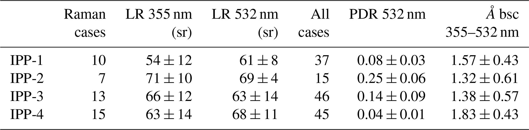
The lidar ratio (LR) at 532 nm and the LR at 355 nm for pollen layers were retrieved using the standard Raman method (Ansmann et al., 1990) during night-time measurements. The mean values are reported in Table 4, and box plots of LR at 532 nm and ratio of LRs are shown in Fig. 10a and b. Although the number of available profiles is limited, our results indicate that pollen consists of medium- to high-absorbing particles with values from 55 to 70 sr for all pollen types. For birch-dominant IPP-1 and nettle-dominant IPP-4, the LR of pollen layers at 532 nm is slightly larger than the LR at 355 nm. This behaviour is reversed for IPP-3 (pine-dominant) and IPP-2 (mixture of birch and spruce). However, no significant wavelength dependence can be determined on LR values accounting for the uncertainties.
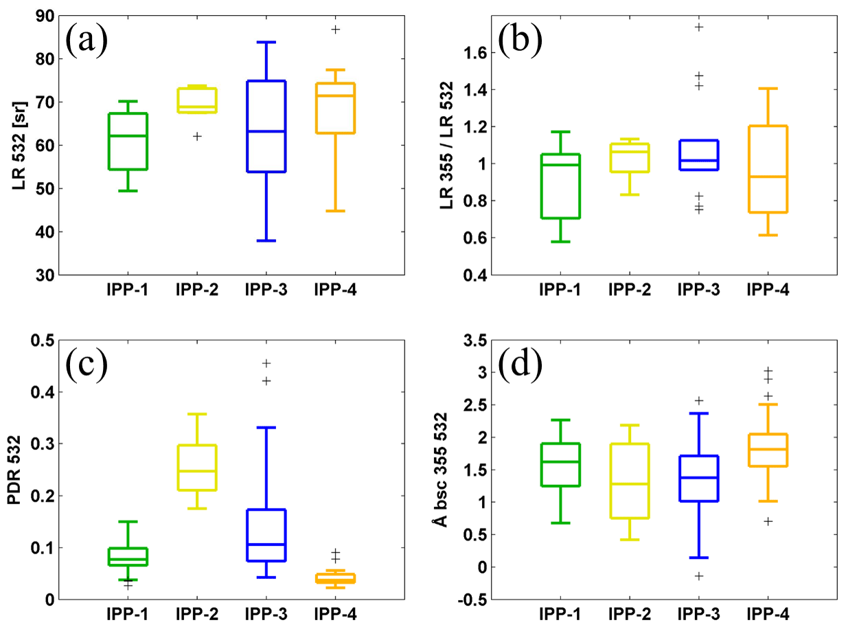
Figure 10Box plots of (a) lidar ratio (LR) at 532 nm and (b) ratio of LR at 355 nm and LR at 532 nm during night-time measurements. Box plots of (c) particle linear depolarization ratio (PDR) and (d) backscatter-related Ångström exponent between 355 and 532 nm during all-day measurements. Mean values of the detected pollen layer for four IPPs are used. The horizontal line represents the median, the boxes the 25 % and 75 % percentiles, the whiskers the standard deviation, and the plus signs the outliers.
The depolarization ratio was clearly enhanced when there were pollen grains in the air, and even higher depolarization ratios were observed with the presence of the more non-spherical spruce and pine pollen. Lidar-derived PDR values of detected pollen layers for the whole periods of each IPP are shown in Table 4 and Fig. 10c. This indicates that the depolarization ratio is the most proper indicator for pollen type. The extinction-related (not shown in this study) and backscatter-related Ångström exponent were also retrieved for pollen layers. The difference in the Ångström exponent for IPPs is much less evident, as the box plot of backscatter-related Ångström exponent between 355 and 532 nm shows (Fig. 10d). The use of the Ångström exponent to characterize pollen is quite delicate, as its value depends a lot on the background aerosol. Nevertheless, a clear tendency to a smaller Ångström exponent with an increasing depolarization ratio can be found, as is reported in Bohlmann et al. (2019). Thus under the same or similar background conditions, the Ångström exponent can be an indicator for pollen type. Even though we assumed that pollen grains were evenly distributed inside the pollen layer, a bigger pollen contribution in the aerosol mixture near the ground was observed.
4.3 Estimation of optical properties for pure pollen from lidar observations
So far, we have retrieved the optical properties of the pollen layers, but the values for pure pollen are still unknown. In this section, the novel methodology presented in Sect. 3 is applied to the real lidar observations to estimate the optical properties for pure pollen particles.
4.3.1 Pollen optical properties at 532 nm
The method given in the inverse model module was applied to the real lidar observations in this section to retrieve the depolarization ratio at 532 nm for pure pollen. We assume that there are only pollen and non-depolarizing background aerosols in the air, which is reasonable because of the clean aerosol conditions at the measurement site.
For the first step, the depolarization ratio of pure pollen (δx) at 532 nm was assumed to be 0.2, 0.3, 0.4, or 0.5, and the depolarization ratio of non-pollen particles (δbackground) at 532 nm was assumed to be 0.03. Under each assumption, we calculated the pollen backscatter coefficient during all IPPs and thus extract the related pollen backscatter contribution inside the pollen layer (χpollen(δx,532)). Mean values of backscatter-related Ångström exponents between 355 and 532 nm inside the pollen layer were retrieved and denoted as Å(355,532). The relationship of Å(355,532) and χpollen(δx,532) of the pollen layers in each IPP was investigated using the parameter η (Eq. 6). The scatter plots using mean η and χpollen(δx,532) under different values of assumed δx (0.2, 0.3, 0.4, or 0.5) for IPP-1 and IPP-3 are given in the Supplement (Fig. S5 for IPP-1 and in Fig. S6 for IPP-3).
Based on results from the first step, in the second step, more δx values between 0.2 and 0.3 for IPP-1 (between 0.3 and 0.4 for IPP-3) were used for the calculations. Linear fitting lines were generated for the η and χpollen(δx,532) (Eq. 8) under each assumed δx. For these fitting lines, the η value for was retrieved, denoted as ηpure(δx,532) and reported in Fig. 11. ηpure presents the η values when the pollen contribution in the observed aerosol particle population is 100 %. Using these estimated ηpure(δx,532) and δx, linear fits (shown by dotted lines in Fig. 11) can be assessed with high correlations.
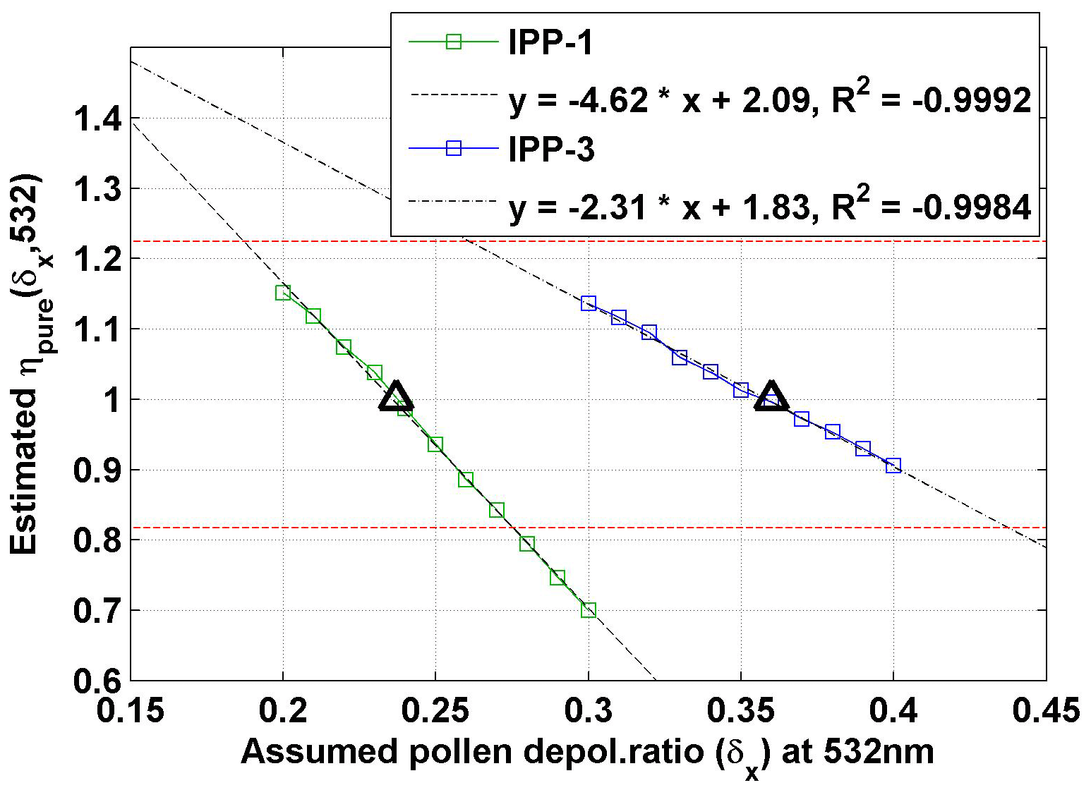
Figure 11Estimated ηpure against the related assumed pollen depolarization ratio δx at 532 nm for IPP-1 (in green) and IPP-3 (in blue). Linear regression lines are drawn by dotted lines, with fitting equations shown. The correlation coefficient (R2) values are also given. η is a parameter using backscatter-related Ångström exponents between 355 and 532 nm (Eq. 6), and ηpure is the estimated η value for χpollen(δx)=1 (i.e. the pollen contribution in the observed aerosol particle population is 100 %) (Eq. 8). The final results for pure pollen are shown by the black triangles. ηpure values of 0.82 and 1.22 (i.e. backscatter-related Ångström exponent of −0.5 and 0.5) are shown by horizontal dotted red lines.
Further on, the δx value which results in a certain value of ηpure(δx,532) could be assumed as the depolarization ratio value of pure pollen. Under the assumption that the backscatter-related Ångström exponent of pure pollen (denoted as Åpollen) between 355 and 532 nm is 0 (i.e. ηpure=1), depolarization ratios of 0.24 or 0.36 were found for IPP-1 or IPP-3, respectively, which are related to the pure birch or pure pine pollen (Table 5). The scatter plots of mean η and χpollen(δx,532) are shown in Fig. 12: (a) for IPP-1 with a pollen depolarization ratio of 0.24 and (b) for IPP-3 with a pollen depolarization ratio of 0.36. Good linear regression relationships are found for both cases, and two things should be highlighted: (1) Åpollen is 0 (i.e. ηpure=1) for 100 % pollen in the observed aerosol particle population (i.e. χpollen=1); and (2) without pollen in the air (i.e. χpollen=0), the backscatter-related Ångström exponent of non-pollen particles (Åbackground) between 355 and 532 nm can be calculated, resulting in values of 2.0 for IPP-1 and 1.9 for IPP-3 (i.e. η of 2.28 for IPP-1, 2.18 for IPP-3). There are no values of the Ångström exponent for pure pollen in the literature, but this assumption (Åpollen=0) is almost realistic, as pollen grains are quite big and thus can be assumed to be wavelength-independent of the backscatter at wavelengths of 355 and 532 nm. For big particles such as dust, Mamouri and Ansmann (2014) reported extinction-related Ångström exponents between 440 and 675 nm, with values of −0.2 for coarse dust and 0.25 for total dust.
Table 5Linear depolarization ratios for pure pollen. The assumption that the backscatter-related Ångström exponent between 355 and 532 nm for pollen (Åpollen) should be 0 was applied for this study. The uncertainty on Åpollen was not taken into account for the standard deviation shown here, which may introduce non-negligible additional bias. For example, under the assumption of Åpollen ± 0.5, the range of depolarization ratio values is 0.19 to 0.27 for birch pollen and 0.26 to 0.44 for pine pollen. See more details in Sect. 4.3.
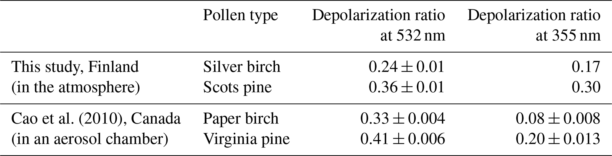
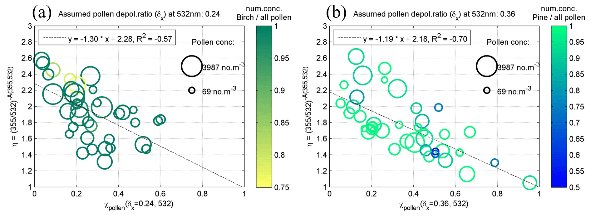
Figure 12Mean values of the parameter η against pollen backscatter contribution at 532 nm (χpollen(δx,532)) inside the pollen layers, during IPP-1 (a) and IPP-3 (b). η is a parameter using the backscatter-related Ångström exponent between 355 and 532 nm (Eq. 6). The pollen depolarization ratio δx at 532 nm is assumed to be 0.24 for (a) or 0.36 for (b). Linear regression lines are drawn by dotted lines, with fitting equation shown (Eqs. 5 or 8). The correlation coefficient (R2) is also given. The size denotes the total pollen concentrations measured by the Burkard sampler at roof level; the colour represents the number concentration of the dominant pollen (a: birch, b: pine) against the total pollen number concentration. Similar figures using different assumed values of pollen depolarization ratio can be found in the Supplement (Figs. S5 and S6).
An uncertainty study was investigated based on the method described in Sect. 3.3 using a Monte Carlo approach. The overall relative uncertainties of the lidar-derived backscatter coefficients are of the order of 5 %–10 % (Baars et al., 2012); we took 10 % here in the simulation. Initial pollen depolarization ratio values were selected to be 0.24 for birch and 0.36 for pine for the uncertainty simulation; initial backscatter-related Ångström exponents of non-pollen particles between 355 and 532 nm were selected to be 2.0 and 1.9 for IPP-1 and IPP-3, respectively. Based on the lidar observations (Fig. 12), the simulated cases were selected so that the χpollen values range from 2 % to 60 % for birch and 2 % to 90 % for pine. The initial input Åpollen in the direct model and assumed in the inverse mode were both selected to be 0. Estimated uncertainties were found to be 2.4 % for birch and 2.9 % for pine (Table 5). Note that the different initial input values of Åpollen may introduce important additional bias. If we assume the true value of Åpollen is between −0.5 and 0.5 (i.e. values of ηpure from 0.82 to 1.22, shown by dotted red lines in Fig. 11), depolarization ratios of 0.19 to 0.27 can be found for birch pollen, and 0.26 to 0.44 can be found for pine pollen. The optical properties of pure pollen are lacking in the literature. Cao et al. (2010) measured the linear depolarization ratio of different pollen types in an aerosol chamber, by disseminating 2 g of the selected pollen; they determined a linear depolarization ratio at 532 nm for paper birch of 0.33 and for Virginia pine of 0.41. These values are higher than what we retrieved in this study, but it has to be kept in mind that these two experiments were conducted in quite different environments and conditions.
The retrieval of depolarization ratios for pure spruce or pure nettle pollen was not possible with this data set. During IPP-2, there was always a mixture of birch and spruce pollen with a variable mixing rate; in addition, the number of available measurements is limited. For nettle pollen, we have observed relatively small depolarization ratio values, together with a small variation, which makes the separation more challenging.
4.3.2 Pollen optical properties at 1064 and 355 nm
A similar study was performed to investigate the relationship between backscatter-related Ångström exponents between 532 and 1064 nm (Å(1064,532)) and the pollen backscatter contribution at 532 nm; here we use another parameter η′ (Eq. 6), which is a function of Å(1064,532), for the total particle backscatter. From the earlier simulations, we found out that the pollen backscatter contribution at 532 nm (χpollen(532)) is proportional to the parameter η′, considering Eq. (5) using the wavelength pair of λ1=1064 and λ2=532.
The inverse model was applied for several assumed pollen depolarization ratios at 532 nm (ranging from 0.2 to 0.6), and no values of (i.e. ) were found (Figs. S5, S6, S7). This result may be due to the fact that the laser beam at longer wavelengths would be more sensitive to bigger particles (pollen). Thus, there is some wavelength dependence on the backscattering between 532 and 1064 nm. The backscatter-related Ångström exponent of non-pollen particles between 532 and 1064 nm, denoted as Åbackground(532,1064), can be calculated using Eq. (5) and the fitting equations in Figs. S5b and S6b, considering no pollen in the air (i.e. χpollen=0). A Åbackground(532,1064) value of 1.0 or 1.1 (i.e. or 0.46) was estimated for IPP-1 or IPP-3, respectively. Considering the previously estimated depolarization ratio at 532 nm for pure birch (pine) pollen of 0.24 (0.36), the related η′ was found to be 0.58 (0.69), corresponding to the value of ∼0.8 (∼0.5) for the backscatter-related Ångström exponent between 532 and 1064 nm. The extinction-related Ångström exponent is characterized mainly by the particle size, whereas the backscatter-related Ångström exponent depends on both the particle size and the refractive index (e.g. Amiridis et al., 2009; Giannakaki et al., 2010). Veselovskii et al. (2015) reported that the backscatter-related Ångström exponent between 355 and 532 nm is more sensitive to the refractive index, compare to the one between 532 and 1064 nm. In a study of Asian dust, Hofer et al. (2020) showed a larger range of values (−0.5 to 1.8) for the 355–532 nm backscatter-related Ångström exponent compared to the 532–1064 nm one (0.1 to 1.4).
A depolarization ratio at 355 nm can also be estimated, as pollen backscatter at both 355 and 532 nm should be the same under the assumption that the backscatter-related Ångström exponent between 355 and 532 nm for pure pollen is 0. The pollen backscatter contribution at 355 nm (χpollen(355)) was calculated using the lidar-derived particle backscatter coefficient at 355 nm. The inverse model was applied here for the backscatter-related Ångström exponent between 355 and 532 nm (Å(532,355)) and pollen backscatter contribution at 355 nm, using a third parameter (as in Eq. 6, a function of Å(532,355)), which is proportional to the pollen backscatter contribution at 355 nm, considering Eq. (5) using the wavelength pair of λ1=532 and λ2=355. Here Å is the backscatter-related Ångström exponent between 355 and 532 nm, for the total particle backscatter coefficient. Under different values of assumed pollen depolarization ratio at 355 nm (δx,355) from 0.1 to 0.4, linear correlations were found for and (Fig. S8). Values for for 100 % pollen backscatter contribution at 355 nm are reported in Fig. 13, against related δx,355. Finally, the pollen depolarization ratios of 0.17 and 0.30 at 355 nm were found for IPP-1 (birch) and IPP-3 (pine), respectively (Table 5). Cao et al. (2010) found smaller values, with a linear depolarization ratio at 355 nm of 0.08 for paper birch and of 0.20 for Virginia pine.
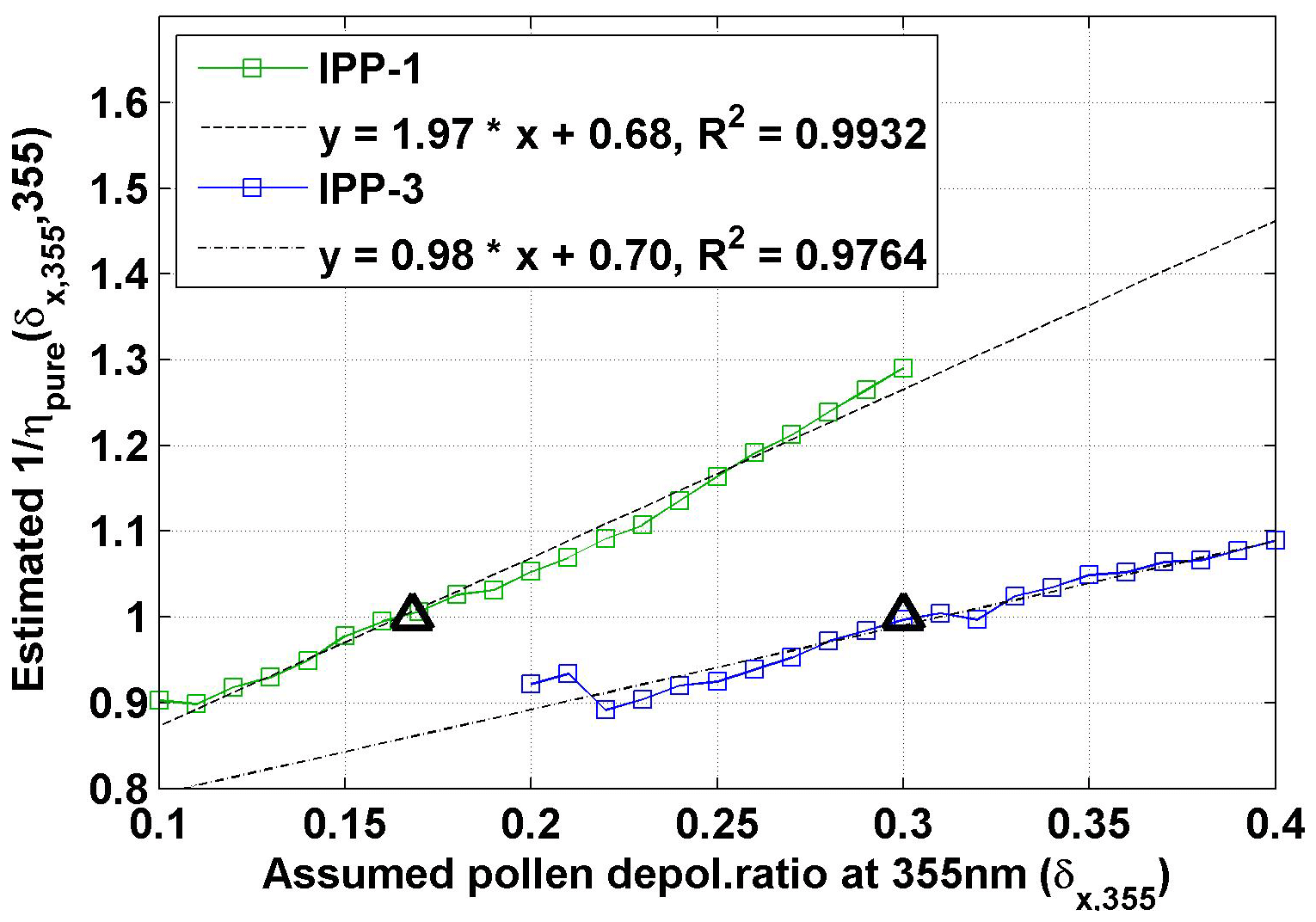
Figure 13Estimated against the related assumed pollen depolarization ratio at 355 nm (δx,355) for IPP-1 (in green) and IPP-3 (in blue). Linear regression lines are drawn by dotted lines, with fitting equations shown. The correlation coefficient (R2) values are also given. is a parameter using the backscatter-related Ångström exponent between 355 and 532 nm (Eq. 6), and is the estimated value for . The final results for pure pollen are shown by the black triangles. Results are under the assumption that the backscatter-related Ångström exponent between 355 and 532 nm for pure pollen is 0.
The particle linear depolarization ratio at 355 nm can be calculated by using the pollen depolarization ratio at 355 nm. Mean values of depolarization ratio of pollen layers for IPP-1 and IPP-3 were retrieved and are shown in Fig. 14. For both periods, PDR values at 355 nm are relatively smaller than the ones at 532 nm.
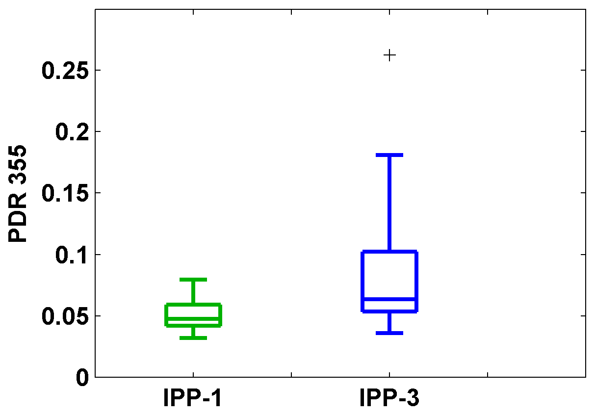
Figure 14Box plots of estimated particle linear depolarization ratio (PDR) at 355 nm. Mean values of the detected pollen layer for all IPPs are used. The horizontal line represent the median, the boxes the 25 % and 75 % percentiles, the whiskers the standard deviation, and the plus signs the outliers. Results are under the assumption that the backscatter-related Ångström exponent between 355 and 532 nm for pure pollen is 0.
Uncertainty values for pollen depolarization ratios and particle linear depolarization ratio at 355 nm are not given in this paper, as these estimations were under the assumption that the backscatter-related Ångström exponent between 355 and 532 nm for pure pollen is 0 and are based on previously retrieved pollen depolarization ratios at 532 nm. More uncertainty sources should be considered for the uncertainty study, and it is complicated to give qualitative values. Nevertheless, a wavelength dependence seems to be found for depolarization values when pollen is present, which may be a key parameter for pollen recognition and characterization. Thus, depolarization ratios at different wavelengths are needed to identify different pollen types.
We have defined lidar-derived properties for pure pollen based on a 4-month pollen campaign, which was performed during May to August 2016 at the Kuopio station in Eastern Finland. This station is part of the European Aerosol Research Lidar Network (EARLINET). Twenty types of pollen were observed and identified by a Burkard sampler, among which birch (Betula), pine (Pinus), spruce (Picea), and nettle (Urtica) pollen were the most abundant, contributing more than 90 % of the total pollen load, regarding number concentrations. Four intense pollination periods (IPPs) were defined considering the pollen seasons and the daily mean pollen concentration values.
Mean values of lidar-derived optical properties in the pollen layer were used to characterize pollen for each IPP. We found that lidar ratio (LR) values range from 55 to 70 sr for all pollen types, indicating that pollen consists of medium- to high-absorbing particles. No significant wavelength dependence could be determined on LR values using LRs at 355 and 532 nm, regarding the uncertainties. The wide range of LRs suggests that the LR alone is not a suitable parameter to discriminate between different pollen types. Nonetheless, we showed that the depolarization ratio is the most proper indicator for pollen and, further, the pollen type, as the depolarization ratio was enhanced when there was pollen in the air, and an even higher depolarization ratio was observed with the presence of the more non-spherical spruce and pine pollen. The Ångström exponent could be used to classify different pollen types only under the same or similar background conditions, as its value depends a lot on the background aerosols.
As the main results, we provide a novel method for the characterization of pure pollen particles. We present an algorithm to estimate the depolarization values for pure pollen, under the assumption that the backscatter-related Ångström exponent between 355 and 532 nm should be zero for pure pollen, as pollen grains are quite large and can be assumed to be wavelength-independent at these two wavelengths. This algorithm was first tested and validated through a simulator of synthetic lidar profiles (including a direct model and an inverse model module). Mathematically, the depolarization ratio for pure pollen can be calculated using the equations given in Sect. 3, if other variables are known or can be assumed. We have developed a retrieval method to estimate the pollen depolarization ratio, which was applied to the lidar observations. The depolarization ratio of pure pollen particles at 532 nm was assessed, resulting in 0.24±0.01 and 0.36±0.01 for birch and pine pollen, respectively. The uncertainty on the assumed backscatter-related Ångström exponent of pure pollen will introduce non-negligible bias in addition, as discussed in Sect. 4.3.1. Pollen optical properties at 1064 and 355 nm were also estimated based on the retrieved pollen depolarization ratio at 532 nm. Pollen depolarization ratios of 0.17 and 0.30 at 355 nm were found for birch and pine pollen, respectively. The depolarization values show a wavelength dependence for pollen. This can be the key parameter for pollen detection and characterization. Also, a wavelength dependence on the backscatter between 532 and 1064 nm was found, with the value of the backscatter-related Ångström exponent of ∼0.8 (∼0.5) for pure birch (pine) pollen between 532 and 1064 nm. Based on simulations in this study, we found that depolarization ratios at 355 nm and 1064 nm provide valuable information for pollen study; thus more multi-wavelength lidar studies on the depolarization characterization of atmospheric pollen are necessary. The presented novel algorithm and the estimated optical properties for pure pollen in this study provide a good method for pollen characterization and classification. Currently, the CALIPSO (Cloud-Aerosol LIdar with Orthogonal Polarization) aerosol type classification scheme includes seven tropospheric aerosol types (Kim et al., 2018; https://www-calipso.larc.nasa.gov/resources/calipso_users_guide/data_summaries/vfm/index_v420.php, last access: 7 April 2020), in which pollen (or biogenic aerosols in general) is excluded. Such ground-based lidar measurements also provide the possibility of implementing a new aerosol type in the CALIPSO classification scheme, for example using the depolarization ratio at 532 nm. This method can also be applied to other aerosol mixtures (e.g. dust and non-dust aerosols) to retrieve the particle linear depolarization ratio related to aerosol types, under the condition that the depolarization ratio of one aerosol type is the only unknown parameter, and other parameters are known or can be reasonably well approximated. Note that the two constraints mentioned in Sect. 3.1 should be considered: both the depolarization ratio and the backscatter-related Ångström exponent of the two aerosol types should be different.
Lidar data are available upon request from the authors, and data quick-looks are available on the PollyNET website (http://polly.tropos.de/, last access: 25 June 2020).
The supplement related to this article is available online at: https://doi.org/10.5194/acp-20-15323-2020-supplement.
XS analysed the data, developed the algorithm and the simulator, and wrote the paper. XS, EG, MK, and SR conceptualized and finalized the methodology. XS and SB performed the lidar data analysis. AS analysed the pollen samples. MK and EG initiated and managed the project. MF, AR, AL, and MK participated in the measurement campaign. All authors were involved in the editing of the paper, interpretation of the results, and discussion of the manuscript.
The authors declare that they have no conflict of interest.
This article is part of the special issue “EARLINET aerosol profiling: contributions to atmospheric and climate research”. It is not associated with a conference.
The authors are thankful for the use of the microphotographs of pollen grains from PalDat (PalDat – a palynological database, 2000 onwards; https://www.paldat.org, last access: 7 April 2020), courtesy of the Division of Structural and Functional Botany, University of Vienna. Elina Giannakaki acknowledges the support of the Hellenic Foundation for Research and Innovation (H.F.R.I.) under the “First Call for H.F.R.I. Research Projects to support Faculty members and Researchers and the procurement of high-cost research equipment grant” (project number: 2544).
This research has been supported by the Academy of Finland (projects no. 310312 and 329216).
This paper was edited by Albert Ansmann and reviewed by three anonymous referees.
Amiridis, V., Balis, D. S., Giannakaki, E., Stohl, A., Kazadzis, S., Koukouli, M. E., and Zanis, P.: Optical characteristics of biomass burning aerosols over Southeastern Europe determined from UV-Raman lidar measurements, Atmos. Chem. Phys., 9, 2431–2440, https://doi.org/10.5194/acp-9-2431-2009, 2009.
Ångström, A.: The parameters of atmospheric turbidity, Tellus A, 16, 64–75, https://doi.org/10.3402/tellusa.v16i1.8885, 1964.
Ansmann, A., Riebesell, M., and Weitkamp, C.: Measurement of atmospheric aerosol extinction profiles with a Raman lidar, Opt. Lett., 15, 746–748, https://doi.org/10.1364/OL.15.000746, 1990.
Ansmann, A., Wandinger, U., Riebesell, M., Weitkamp, C., and Michaelis, W.: Independent measurement of extinction and backscatter profiles in cirrus clouds by using a combined Raman elastic-backscatter lidar, Appl. Optics, 31, 7113–7131, 1992.
Baars, H., Ansmann, A., Althausen, D., Engelmann, R., Heese, B., Müller, D., Artaxo, P., Paixao, M., Pauliquevis, T., and Souza, R.: Aerosol profiling with lidar in the Amazon Basin during the wet and dry season, J. Geophys. Res.-Atmos., 117, D21201, https://doi.org/10.1029/2012JD018338, 2012.
Bohlmann, S., Shang, X., Giannakaki, E., Filioglou, M., Saarto, A., Romakkaniemi, S., and Komppula, M.: Detection and characterization of birch pollen in the atmosphere using a multiwavelength Raman polarization lidar and Hirst-type pollen sampler in Finland, Atmos. Chem. Phys., 19, 14559–14569, https://doi.org/10.5194/acp-19-14559-2019, 2019.
Bösenberg, J. and Matthias, V.: EARLINET: A European Aerosol Research Lidar Network to Establish an Aerosol Climatology, MPI Rep., 348, 6–31, 2003.
Bousquet, J., Khaltaev, N., Cruz, A. A., Denburg, J., Fokkens, W. J., Togias, A., Zuberbier, T., Baena-Cagnani, C. E., Canonica, G. W., Van Weel, C., Agache, I., Aït-Khaled, N., Bachert, C., Blaiss, M. S., Bonini, S., Boulet, L.-P., Bousquet, P.-J., Camargos, P., Carlsen, K.-H., Chen, Y., Custovic, A., Dahl, R., Demoly, P., Douagui, H., Durham, S. R., Van Wijk, R. G., Kalayci, O., Kaliner, M. A., Kim, Y.-Y., Kowalski, M. L., Kuna, P., Le, L. T. T., Lemiere, C., Li, J., Lockey, R. F., Mavale-Manuel, S., Meltzer, E. O., Mohammad, Y., Mullol, J., Naclerio, R., O'Hehir, R. E., Ohta, K., Ouedraogo, S., Palkonen, S., Papadopoulos, N., Passalacqua, G., Pawankar, R., Popov, T. A., Rabe, K. F., Rosado-Pinto, J., Scadding, G. K., Simons, F. E. R., Toskala, E., Valovirta, E., Van Cauwenberge, P., Wang, D.-Y., Wickman, M., Yawn, B. P., Yorgancioglu, A., Yusuf, O. M., Zar, H., Annesi-Maesano, I., Bateman, E. D., Ben Kheder, A., Boakye, D. A., Bouchard, J., Burney, P., Busse, W. W., Chan-Yeung, M., Chavannes, N. H., Chuchalin, A., Dolen, W. K., Emuzyte, R., Grouse, L., Humbert, M., Jackson, C., Johnston, S. L., Keith, P. K., Kemp, J. P., Klossek, J.-M., Larenas-Linnemann, D., Lipworth, B., Malo, J.-L., Marshall, G. D., Naspitz, C., Nekam, K., Niggemann, B., Nizankowska-Mogilnicka, E., Okamoto, Y., Orru, M. P., Potter, P., Price, D., Stoloff, S. W., Vandenplas, O., Viegi, G., and Williams, D.: Allergic Rhinitis and its Impact on Asthma (ARIA) 2008*, Allergy, 63, 8–160, https://doi.org/10.1111/j.1398-9995.2007.01620.x, 2008.
Buters, J. T. M., Antunes, C., Galveias, A., Bergmann, K. C., Thibaudon, M., Galán, C., Schmidt-Weber, C., and Oteros, J.: Pollen and spore monitoring in the world, Clin. Transl. Allergy, 8, 9, https://doi.org/10.1186/s13601-018-0197-8, 2018.
Cao, X., Roy, G., and Bernier, R.: Lidar polarization discrimination of bioaerosols, Opt. Eng., 49, 116201, https://doi.org/10.1117/1.3505877, 2010.
D'Amato, G., Cecchi, L., Bonini, S., Nunes, C., Annesi-Maesano, I., Behrendt, H., Liccardi, G., Popov, T., and van Cauwenberge, P.: Allergenic pollen and pollen allergy in Europe, Allergy, 62, 976—990, https://doi.org/10.1111/j.1398-9995.2007.01393.x, 2007.
Eck, T. F., Holben, B. N., Reid, J. S., Dubovik, O., Smirnov, A., O'Neill, N. T., Slutsker, I., and Kinne, S.: Wavelength dependence of the optical depth of biomass burning, urban, and desert dust aerosols, J. Geophys. Res.-Atmos., 104, 31333–31349, https://doi.org/10.1029/1999JD900923, 1999.
Engelmann, R., Kanitz, T., Baars, H., Heese, B., Althausen, D., Skupin, A., Wandinger, U., Komppula, M., Stachlewska, I. S., Amiridis, V., Marinou, E., Mattis, I., Linné, H., and Ansmann, A.: The automated multiwavelength Raman polarization and water-vapor lidar PollyXT: the neXT generation, Atmos. Meas. Tech., 9, 1767–1784, https://doi.org/10.5194/amt-9-1767-2016, 2016.
Fernald, F. G.: Analysis of atmospheric lidar observations: some comments, Appl. Optics, 23, 652–653, 1984.
Flamant, C., Pelon, J., Flamant, P. H., and Durand, P.: Lidar determination of the entrainment zone thickness at the top of the unstable marine atmospheric boundary layer, Bound.-Lay. Meteorol., 83, 247–284, https://doi.org/10.1023/A:1000258318944, 1997.
Giannakaki, E., Balis, D. S., Amiridis, V., and Zerefos, C.: Optical properties of different aerosol types: seven years of combined Raman-elastic backscatter lidar measurements in Thessaloniki, Greece, Atmos. Meas. Tech., 3, 569–578, https://doi.org/10.5194/amt-3-569-2010, 2010.
Giesecke, T., Fontana, S. L., van der Knaap, W. O., Pardoe, H. S., and Pidek, I. A.: From early pollen trapping experiments to the Pollen Monitoring Programme, Veg. Hist. Archaeobot., 19, 247–258, https://doi.org/10.1007/s00334-010-0261-3, 2010.
Goldberg, C., Buch, H., Moseholm, L., and Weeke, E. R.: Airborne Pollen Records in Denmark, 1977–1986, Grana, 27, 209–217, https://doi.org/10.1080/00173138809428928, 1988.
Hirsikko, A., O'Connor, E. J., Komppula, M., Korhonen, K., Pfüller, A., Giannakaki, E., Wood, C. R., Bauer-Pfundstein, M., Poikonen, A., Karppinen, T., Lonka, H., Kurri, M., Heinonen, J., Moisseev, D., Asmi, E., Aaltonen, V., Nordbo, A., Rodriguez, E., Lihavainen, H., Laaksonen, A., Lehtinen, K. E. J., Laurila, T., Petäjä, T., Kulmala, M., and Viisanen, Y.: Observing wind, aerosol particles, cloud and precipitation: Finland's new ground-based remote-sensing network, Atmos. Meas. Tech., 7, 1351–1375, https://doi.org/10.5194/amt-7-1351-2014, 2014.
Hirst, J. M.: An automatic volumetric spore trap, Ann. Appl. Biol., 39, 257–265, https://doi.org/10.1111/j.1744-7348.1952.tb00904.x, 1952.
Hofer, J., Ansmann, A., Althausen, D., Engelmann, R., Baars, H., Fomba, K. W., Wandinger, U., Abdullaev, S. F., and Makhmudov, A. N.: Optical properties of Central Asian aerosol relevant for spaceborne lidar applications and aerosol typing at 355 and 532 nm, Atmos. Chem. Phys., 20, 9265–9280, https://doi.org/10.5194/acp-20-9265-2020, 2020
Holt, K. A. and Bennett, K. D.: Principles and methods for automated palynology, New Phytol., 203, 735–742, https://doi.org/10.1111/nph.12848, 2014.
Illingworth, A. J., Barker, H. W., Beljaars, A., Ceccaldi, M., Chepfer, H., Clerbaux, N., Cole, J., Delanoë, J., Domenech, C., Donovan, D. P., Fukuda, S., Hirakata, M., Hogan, R. J., Huenerbein, A., Kollias, P., Kubota, T., Nakajima, T., Nakajima, T. Y., Nishizawa, T., Ohno, Y., Okamoto, H., Oki, R., Sato, K., Satoh, M., Shephard, M. W., Velázquez-Blázquez, A., Wandinger, U., Wehr, T., van Zadelhoff, G.-J.: The EarthCARE Satellite: The Next Step Forward in Global Measurements of Clouds, Aerosols, Precipitation, and Radiation, B. Am. Meteorol. Soc., 96, 1311–1332, https://doi.org/10.1175/BAMS-D-12-00227.1, 2015.
Kim, M.-H., Omar, A. H., Tackett, J. L., Vaughan, M. A., Winker, D. M., Trepte, C. R., Hu, Y., Liu, Z., Poole, L. R., Pitts, M. C., Kar, J., and Magill, B. E.: The CALIPSO version 4 automated aerosol classification and lidar ratio selection algorithm, Atmos. Meas. Tech., 11, 6107–6135, https://doi.org/10.5194/amt-11-6107-2018, 2018.
Klett, J. D.: Stable analytical solution for processing lidar returns, Appl. Optics, 20, 211–220, 1981.
Mamouri, R. E. and Ansmann, A.: Fine and coarse dust separation with polarization lidar, Atmos. Meas. Tech., 7, 3717–3735, https://doi.org/10.5194/amt-7-3717-2014, 2014.
Mattis, I., Müller, D., Ansmann, A., Wandinger, U., Preißler, J., Seifert, P., and Tesche, M.: Ten years of multiwavelength Raman lidar observations of free-tropospheric aerosol layers over central Europe: Geometrical properties and annual cycle, J. Geophys. Res., 113, D20202, https://doi.org/10.1029/2007JD009636, 2008.
Miguel, A. G., Taylor, P. E., House, J., Glovsky, M. M., and Flagan, R. C.: Meteorological Influences on Respirable Fragment Release from Chinese Elm Pollen, Aerosol Sci. Technol., 40, 690–696, https://doi.org/10.1080/02786820600798869, 2006.
Nilsson, S. T., Siwert, T., Praglowski, J., and Nilsson, L.: Atlas of airborne pollen grains and spores in northern Europe, availabe at: https://agris.fao.org/agris-search/search.do?recordID=SE7801026 (last access: 17 June 2020), 1977.
Noh, Y. M., Lee, H., Mueller, D., Lee, K., Shin, D., Shin, S., Choi, T. J., Choi, Y. J., and Kim, K. R.: Investigation of the diurnal pattern of the vertical distribution of pollen in the lower troposphere using LIDAR, Atmos. Chem. Phys., 13, 7619–7629, https://doi.org/10.5194/acp-13-7619-2013, 2013.
Rousseau, D.-D., Schevin, P., Ferrier, J., Jolly, D., Andreasen, T., Ascanius, S. E., Hendriksen, S.-E., and Poulsen, U.: Long-distance pollen transport from North America to Greenland in spring, J. Geophys. Res.-Biogeo., 113, G02013, https://doi.org/10.1029/2007JG000456, 2008.
Schmeisser, L., Backman, J., Ogren, J. A., Andrews, E., Asmi, E., Starkweather, S., Uttal, T., Fiebig, M., Sharma, S., Eleftheriadis, K., Vratolis, S., Bergin, M., Tunved, P., and Jefferson, A.: Seasonality of aerosol optical properties in the Arctic, Atmos. Chem. Phys., 18, 11599–11622, https://doi.org/10.5194/acp-18-11599-2018, 2018.
Schmidt, C. W.: Pollen Overload: Seasonal Allergies in a Changing Climate, Environ. Health Perspect., 124, 70–75, https://doi.org/10.1289/ehp.124-A70, 2016.
Shang, X. and Chazette, P.: End-to-end simulation for a forest-dedicated full-waveform lidar onboard a satellite initialized from airborne ultraviolet lidar experiments, Remote Sens., 7, 5222–5255, https://doi.org/10.3390/rs70505222, 2015.
Shang, X., Chazette, P., and Totems, J.: Analysis of a warehouse fire smoke plume over Paris with an N2 Raman lidar and an optical thickness matching algorithm, Atmos. Meas. Tech., 11, 6525–6538, https://doi.org/10.5194/amt-11-6525-2018, 2018.
Sicard, M., Izquierdo, R., Alarcón, M., Belmonte, J., Comerón, A., and Baldasano, J. M.: Near-surface and columnar measurements with a micro pulse lidar of atmospheric pollen in Barcelona, Spain, Atmos. Chem. Phys., 16, 6805–6821, https://doi.org/10.5194/acp-16-6805-2016, 2016.
Skjøth, C. A., Sommer, J., Stach, A., Smith, M., and Brandt, J.: The long-range transport of birch (Betula) pollen from Poland and Germany causes significant pre-season concentrations in Denmark, Clin. Exp. Allergy, 37, 1204–1212, https://doi.org/10.1111/j.1365-2222.2007.02771.x, 2007.
Sofiev, M., Berger, U., Prank, M., Vira, J., Arteta, J., Belmonte, J., Bergmann, K.-C., Chéroux, F., Elbern, H., Friese, E., Galan, C., Gehrig, R., Khvorostyanov, D., Kranenburg, R., Kumar, U., Marécal, V., Meleux, F., Menut, L., Pessi, A.-M., Robertson, L., Ritenberga, O., Rodinkova, V., Saarto, A., Segers, A., Severova, E., Sauliene, I., Siljamo, P., Steensen, B. M., Teinemaa, E., Thibaudon, M., and Peuch, V.-H.: MACC regional multi-model ensemble simulations of birch pollen dispersion in Europe, Atmos. Chem. Phys., 15, 8115–8130, https://doi.org/10.5194/acp-15-8115-2015, 2015.
Steiner, A. L., Brooks, S. D., Deng, C., Thornton, D. C. O., Pendleton, M. W., and Bryant, V.: Pollen as atmospheric cloud condensation nuclei, Geophys. Res. Lett., 42, 3596–3602, https://doi.org/10.1002/2015GL064060, 2015.
Szczepanek, K., Myszkowska, D., Worobiec, E., Piotrowicz, K., Ziemianin, M., and Bielec-Bkakowska, Z.: The long-range transport of Pinaceae pollen: an example in Kraków (southern Poland), Aerobiologia, 33, 109–125, https://doi.org/10.1007/s10453-016-9454-2, 2017.
Tesche, M., Ansmann, A., Müller, D., Althausen, D., Engelmann, R., Freudenthaler, V., and Groß, S.: Vertically resolved separation of dust and smoke over Cape Verde using multiwavelength Raman and polarization lidars during Saharan Mineral Dust Experiment 2008, J. Geophys. Res., 114, D13202, https://doi.org/10.1029/2009JD011862, 2009.
Tomasi, C., Lupi, A., Mazzola, M., Stone, R. S., Dutton, E. G., Herber, A., Radionov, V. F., Holben, B. N., Sorokin, M. G., Sakerin, S. M., Terpugova, S. A., Sobolewski, P. S., Lanconelli, C., Petkov, B. H., Busetto, M., and Vitale, V.: An update on polar aerosol optical properties using POLAR-AOD and other measurements performed during the International Polar Year, Atmos. Environ., 52, 29–47, https://doi.org/10.1016/j.atmosenv.2012.02.055, 2012.
Veselovskii, I., Whiteman, D. N., Korenskiy, M., Suvorina, A., Kolgotin, A., Lyapustin, A., Wang, Y., Chin, M., Bian, H., Kucsera, T. L., Pérez-Ramírez, D., and Holben, B.: Characterization of forest fire smoke event near Washington, DC in summer 2013 with multi-wavelength lidar, Atmos. Chem. Phys., 15, 1647–1660, https://doi.org/10.5194/acp-15-1647-2015, 2015.
Weber, R. W.: Pollen Identification, Ann. Allergy Asthma Immunol., 80, 141–148, https://doi.org/10.1016/S1081-1206(10)62947-X, 1998.
Yli-Panula, E., Fekedulegn, D. B., Green, B. J., and Ranta, H.: Analysis of Airborne Betula Pollen in Finland, a 31-Year Perspective, Int. J. Environ. Res. Public Health, 6, 1706–1723, https://doi.org/10.3390/ijerph6061706, 2009.