the Creative Commons Attribution 4.0 License.
the Creative Commons Attribution 4.0 License.
 | 08 Dec 2020
Impact of Lagrangian transport on lower-stratospheric transport timescales in a climate model
Edward J. Charlesworth
Ann-Kristin Dugstad
Frauke Fritsch
Patrick Jöckel
Felix Plöger
We investigate the impact of model trace gas transport schemes on the representation of transport processes in the upper troposphere and lower stratosphere. Towards this end, the Chemical Lagrangian Model of the Stratosphere (CLaMS) was coupled to the ECHAM/MESSy Atmospheric Chemistry (EMAC) model and results from the two transport schemes (Lagrangian critical Lyapunov scheme and flux-form semi-Lagrangian, respectively) were compared. Advection in CLaMS was driven by the EMAC simulation winds, and thereby the only differences in transport between the two sets of results were caused by differences in the transport schemes. To analyze the timescales of large-scale transport, multiple tropical-surface-emitted tracer pulses were performed to calculate age of air spectra, while smaller-scale transport was analyzed via idealized, radioactively decaying tracers emitted in smaller regions (nine grid cells) within the stratosphere. The results show that stratospheric transport barriers are significantly stronger for Lagrangian EMAC-CLaMS transport due to reduced numerical diffusion. In particular, stronger tracer gradients emerge around the polar vortex, at the subtropical jets, and at the edge of the tropical pipe. Inside the polar vortex, the more diffusive EMAC flux-form semi-Lagrangian transport scheme results in a substantially higher amount of air with ages from 0 to 2 years (up to a factor of 5 higher). In the lowermost stratosphere, mean age of air is much smaller in EMAC, owing to stronger diffusive cross-tropopause transport. Conversely, EMAC-CLaMS shows a summertime lowermost stratosphere age inversion – a layer of older air residing below younger air (an “eave”). This pattern is caused by strong poleward transport above the subtropical jet and is entirely blurred by diffusive cross-tropopause transport in EMAC. Potential consequences from the choice of the transport scheme on chemistry–climate and geoengineering simulations are discussed.
- Article
(12126 KB) - Full-text XML
- BibTeX
- EndNote


The upper troposphere and lower stratosphere (UTLS) is an important region for global climate as the chemical composition of radiatively active trace gas species there has crucial impacts on radiation and surface temperatures (e.g., Solomon et al., 2010). The entry of air masses into the stratosphere is controlled by the chemical and dynamical processes in the UTLS (e.g., Holton et al., 1995; Fueglistaler et al., 2009), presenting a challenge for understanding and modeling the region. To overcome, climate models must have a realistic representation of UTLS transport processes in order to provide reliable predictions and assist in robust theoretical development. For instance, in simulating the effects of geoengineering by sulfur injections into the stratosphere, uncertainties in the model transport representation could cause substantial uncertainties in the simulations (Tilmes et al., 2018; Kravitz and Douglas, 2020). Even small differences in composition caused by model differences in small-scale transport processes (e.g., turbulence, diffusion) may cause significant model spread in surface temperatures (e.g., Riese et al., 2012). This radiative effect of composition changes in the UTLS is particularly large for water vapor but also substantial for other species like O3, N2O, and CH4.
Critical processes for models are transport around the wintertime stratospheric polar vortex, stratosphere–troposphere exchange across the tropopause, and horizontal exchange between the tropical lower stratosphere (the tropical pipe; Plumb, 1996) and middle latitudes (for reviews of stratospheric transport processes see e.g., Plumb, 2002; Shepherd, 2007). The steep gradients in observed trace gas distributions in these regions are signs of transport barriers and regions of suppressed exchange, for example, around the polar vortex, at the edge of the tropical pipe, and along the extratropical tropopause. The representation of transport processes in the lower stratosphere in global models is prone to numerical diffusion, as tracer distributions in this region are characterized by sharp gradients and frequent small-scale filamentary structures (McKenna et al., 2002).
Atmospheric models (as used in current coupled chemistry–climate models) employ different numerical schemes for solving trace gas transport, all of which introduce some unwanted, unphysical numerical diffusion. Numerical diffusion smoothes gradients and small-scale filaments in tracer distributions, and thereby differences in numerical diffusion cause differences in trace gas transport in different models, affecting the simulated distributions of trace gas species. Research has been focused on this topic for decades, with early work performed by Rood (1987) for one-dimensional flow. Numerical diffusion in multi-dimensional models, using mean age of air as a diagnostic, was studied by both Hall et al. (1999) and Eluszkiewicz et al. (2000), while Gregory and West (2002) performed a similar study focusing on stratospheric water vapor transport. These studies found significantly younger stratospheric mean age of air and a faster water vapor tape recorder propagation for more diffusive transport schemes. Later, Kent et al. (2014) provided a detailed analysis of idealized tracers and transport scenarios. Most recently, Gupta et al. (2020) studied a variety of dynamical cores using mean age of air as a transport diagnostic, demonstrating that many issues with numerical diffusion are still relevant with modern techniques and computational resources.
Most currently used transport schemes are based on a regular grid (e.g., Morgenstern et al., 2010) and will be referred to as Eulerian schemes in the text to follow. Another class of transport schemes, Lagrangian schemes, on the other hand, follow the motion of air parcels through the atmospheric flow and hence have reduced diffusion characteristics due to the absence of interpolations of tracer distributions to a regular grid (e.g., McKenna et al., 2002). Semi-Lagrangian schemes are still based on a regular grid, but they incorporate some advantages of Lagrangian transport by calculating the air motion over one model time step through a Lagrangian advection scheme, but this is then followed by remapping onto the grid. One such scheme which is both sophisticated and frequently used in global models is the flux-form semi-Lagrangian (FFSL) scheme (e.g., Lin and Rood, 1996; Lin, 2004).
Fully Lagrangian transport schemes, by definition, are free of numerical diffusion, as parcels are left entirely isolated from each other when no inter-parcel mixing scheme is applied. Parcel mixing due to small-scale processes (e.g., turbulence) can then be introduced based on physical parameterizations, and the strength of mixing can then be controlled. Due to the complications of handling irregular (air parcel) grids, Lagrangian schemes are not commonly used in global climate models. To our knowledge, the only two Lagrangian transport schemes which are currently implemented in a global climate model are ATTILA (Stenke et al., 2008, 2009; Brinkop and Jöckel, 2019) and CLaMS (Hoppe et al., 2014, 2016). Both these schemes have been integrated into the ECHAM/MESSy Atmospheric Chemistry (EMAC) climate model (e.g., Jöckel et al., 2005, 2016), and at the present time neither has been incorporated into another climate model.
Stenke et al. (2008) showed that using the ATTILA scheme in EMAC reduced the excessive transport of water vapor into the lowermost stratosphere and into polar regions, and the associated cold bias in temperatures could be partly corrected. The representation of stratospheric ozone was also found to have been improved (Stenke et al., 2009). Hoppe et al. (2014) further showed that CLaMS transport within EMAC results in a more realistic representation of transport barriers around the southern polar vortex, due to reduced numerical diffusion compared to the EMAC-FFSL scheme.
Here, we build on the study of Hoppe et al. (2014) and further analyze the implementation of the Lagrangian transport scheme CLaMS within the EMAC climate model. We compare results from two tracer sets within one EMAC simulation: one set where transport is calculated using the EMAC-FFSL scheme and one set using the CLaMS Lagrangian tracer transport scheme. To enable a more detailed analysis of composition and transport timescales, going beyond the average stratospheric transit time (the mean age; Waugh and Hall, 2002) as considered by Hoppe et al. (2014), we calculate the full (time-dependent) stratospheric age of air spectrum (the distribution of stratospheric transit times) of model transport schemes.
This work investigates the differences in transport in the lower stratosphere between these two transport schemes using the age spectrum, mean age, and idealized tracers as diagnostics. The work is focused on identifying the regions that are most sensitive to changes in the tracer transport scheme, assessing the timescales for which the transport schemes differ, and identifying the potential consequences for simulated chemical composition and geoengineering simulations.
In Sect. 2 the used models and diagnostic methods (age spectrum, forward tracers) are introduced. Section 3 presents the results from a global perspective, while Sect. 4 focuses on particular processes and regions. In Sect. 5 the transport scheme differences are discussed against the background of current research on stratospheric geoengineering. The main conclusions are summarized in Sect. 6.
2.1 Models
The model used in this work is EMAC, the MESSy (Modular Earth Submodel System) version of the ECHAM5 climate model (see Jöckel et al., 2010 for details on EMAC and Roeckner et al., 2006 for details on ECHAM5). EMAC is a modern chemistry–climate model which is commonly used for studies of the stratosphere and upper troposphere (Sinnhuber and Meul, 2015; Oberländer-Hayn et al., 2016; Fritsch et al., 2020), as well as studies of the troposphere. In this work, EMAC is operated at the T42L90MA spectral resolution, corresponding to a horizontal quadratic Gaussian grid of approximately resolution with 90 vertical layers. One simulation is performed with this model, by which two sets of time-resolved tracer distributions were calculated. One tracer set was calculated with the standard EMAC-FFSL transport scheme and will be referenced as the Eulerian representation or EMAC-FFSL. The other tracer set was calculated with the CLaMS EMAC submodel and will be referenced as the Lagrangian representation or EMAC-CLaMS.
The EMAC-FFSL transport scheme is the flux-form semi-Lagrangian (FFSL) scheme (Lin and Rood, 1996), which is used in many modern climate models. The EMAC-FFSL vertical coordinate is a hybrid sigma-pressure coordinate, which is another common choice in the development of modern climate models. The time resolution of the EMAC simulation performed in this work is 12 min. The simulation consists of 10 years of spin-up, with a following 10 years of result production. The EMAC version used in this work is 2.53.1, and the model was free-running (i.e., not forced by meteorological fields). Although EMAC can be used for chemistry–climate model simulations, the configuration in this work did not simulate interactive chemical fields. The water vapor field, however, was interactive, and included stratospheric moistening via methane oxidation (see e.g., Revell et al., 2016). Sea-surface temperatures and sea ice were prescribed from the HadISST climatology (Rayner et al., 2003). Meanwhile, CO2, CH4, N2O, CFC-11, and CFC-12 mixing ratios were fixed at 367 ppmv, 175 ppmv, 316 ppbv, 262 pptv, and 520 pptv, respectively, for calculation of radiation. Other details of the EMAC set-up are identical to those of Jöckel et al. (2016).
CLaMS (the Chemical Lagrangian Model of the Stratosphere) is a Lagrangian chemical transport model based on three-dimensional trajectories and an additional mixing parameterization. The EMAC-CLaMS results in this work were produced with a resolution of approximately 3 million air parcels. Unique among Lagrangian models, CLaMS uses a mixing parameterization which is robustly based on physical principles. This parameterization is based on the critical Lyapunov exponent method, details of which can be found in Konopka et al. (2004). The vertical coordinate of CLaMS is a hybrid σ−θ coordinate (referred to as ζ) (Hoppe et al., 2014). Above the prescribed reference pressure of 300 hPa, ζ is identical to θ and therefore the vertical advection velocity throughout the stratosphere is identical to the diabatic heating rate. CLaMS advection is normally driven by horizontal winds and diabatic heating rates from reanalyses (e.g., Konopka et al., 2007; Ploeger et al., 2019); however in EMAC-CLaMS advection of CLaMS parcels is driven by the horizontal winds and heating rates of EMAC. This advection is driven online, during execution of the simulation, so that the underlying velocity fields for advection in EMAC-CLaMS and EMAC-FFSL are exactly the same. However, there are two differences in how these fields are used by the transport schemes. (1) EMAC-CLaMS interpolates the horizontal winds onto parcel locations, whereas EMAC-FFSL uses the winds directly on the EMAC grid points. (2) As mentioned above, the vertical velocity of EMAC-CLaMS is the diabatic heating rate (calculated by EMAC), whereas EMAC-FFSL uses a kinematic vertical velocity (calculated by closure of the mass balance equation). The horizontal and vertical velocities in the two transport schemes are therefore consistent, but not actually identical. More details of EMAC-CLaMS are described by Hoppe et al. (2014, 2016).
2.2 Age spectra
The goal of this work is examination of differences in tracer transport between two advection schemes, for which analysis of passive tracers is ideal. This approach, as opposed to examination of chemically active species, eliminates differences that could arise through the differing chemical schemes of EMAC and the CLaMS submodel of EMAC. The diagnostic tool used in this work is the age spectrum, , which describes the probability distribution of stratospheric transit times τ (age) within an air parcel sampled at location r and time t (e.g., Waugh and Hall, 2002). The first moment of the age spectrum is the mean age Γ, which represents the average transit time from a tracer source region to a given point in the atmosphere
In models, age spectra can be calculated by a series of tracers which are pulsed at some reference location (in this case the tropical surface). For such a tracer with a pulse in the source region at time ti the mixing ratio χi(r, t) at point r and time t can be normalized to the probability density for air of the transit time , which is the value of the age spectrum.
Therefore, a suite of pulse tracers provides the full transit time dependency of the age spectrum function G.
This boundary impulse response method has been used in a few other modeling studies to calculate fully time-dependent stratospheric age spectra (for further details see e.g. Li et al., 2012; Ploeger and Birner, 2016; Hauck et al., 2019). In this work, the tracers are emitted over the course of 30 d, after which emissions are ceased, and one tracer is pulsed every 3 months, specifically in January, April, July, and October of each year, analogous to the set-up by Hauck et al. (2019). Tracer emission is performed by prescribing the surface boundary mixing ratio in EMAC. Each tracer is therefore assigned an age based on when the tracer was emitted, and the combined set of tracers is used to create the age distribution. Forty tracers are utilized in total, such that the calculated age spectra span the course of 10 years. After 10 years, mixing ratios of the oldest tracer are set to zero throughout the model domain and the tracer is re-pulsed, so that the age spectra always span from 0 to 10 years. Furthermore, the spectra are normalized so that the integral of the spectra over transit time always equals 1.
Due to the truncation of the age spectrum at 10 years of age, although a “true” age spectrum would show a significant fraction of air older than 10 years, the mean age is biased young. This fact is important to bear in mind in comparing the mean age described here to calculations in other studies (e.g., Li et al., 2012). It has been shown that the age spectrum tail can be extrapolated to infinity by fitting an exponential decay (e.g., Diallo et al., 2012) and the mean age can be corrected accordingly. However, to facilitate comparison between EMAC-FFSL and EMAC-CLaMS transport, we refrain from applying this tail correction and focus on the resolved part of the age spectrum with transit times younger than 10 years. The uncalculated differences in the spectrum tail at ages older than 10 years are likely small compared to the differences in the resolved section of the spectra.
2.3 Forward tracers
One disadvantage of the analysis of age spectra is abstraction of results away from the transport of realistic chemically active species, such as water and ozone. In the results that follow, considerable differences are found in age spectra between the two considered transport schemes. These results indicate distinct differences in tracer transport but do not directly predict contrasts in the transport of specific, chemically active tracers. We therefore investigate additional idealized trace gas species to reflect the results in a less abstract form. In particular, we consider the case of tracers with the simplest chemistry possible – that of radioactive decay. By convoluting an air parcel's age spectrum with an exponentially decaying weighting, the fraction of a hypothetical radioactive tracer with a decay lifetime T that would remain after transport from the tropical surface (the origin of the pulse tracers) can be calculated
Here, is the tracer mixing ratio at the tropical surface.
Throughout this paper, this quantity will be referred to as a “forward tracer”, as it is computed forward from the knowledge of the age distributions throughout the model domain.
2.4 The EMAC-CLaMS lower and upper boundaries
A critical decision in this study lies in the way in which age tracers are pulsed. Differences in the age spectra between the two transport schemes would ideally stem only from differences in transport within the region of interest (the stratosphere and upper troposphere). As mentioned in the introduction, the two transport schemes differ greatly in the representation of convective transport, as EMAC-CLaMS does not account for parameterized convection, while in the grid-point representation the tracers are subject to a convective transport parameterization. To eliminate the effects of this difference below the upper troposphere, the age tracer concentrations of the EMAC-CLaMS representation were fixed to those of EMAC-FFSL below level 73 of the EMAC model. This level corresponds to 270 hPa (330 K) in the tropics and extratropics and about 250 hPa (300 K) in the winter polar region (poleward of 75 ∘). The procedure is as follows: for each EMAC-CLaMS parcel at each time step, the EMAC grid cell containing the parcel was identified and if the parcel was located at or below EMAC level 73, the EMAC-CLaMS parcel age tracer values were replaced by EMAC-FFSL age tracer values of that EMAC cell. In this way, EMAC-FFSL results do not qualitatively differ from those of EMAC-CLaMS below EMAC level 73 (the upper troposphere). There are, however, small quantitative differences between the two sets of transport scheme results due to interpolation and numerics because the two representations have different grids and resolutions in this region. This creates very minor differences which are most noticeable near the surface.
The model top in EMAC is at 0.01 hPa (approximately 80 km) (Jöckel et al., 2016). As the CLaMS transport scheme has not been extended into the mesosphere so far, the uppermost level in EMAC-CLaMS results is around the stratopause (around 2500 K; see Hoppe et al., 2014). Therefore, in regions of downwelling air from the mesosphere, EMAC-CLaMS age of air will be young-biased compared to the EMAC-FFSL age. However, as this paper focuses on the lower stratosphere, the effect of these differences is expected to be weak. Furthermore, as the EMAC-CLaMS age is found to be generally older than the EMAC-FFSL age in the lower stratosphere (see Fig. 1), these age differences can be regarded as conservative estimates of inter-representation differences.
3.1 Mean age of air
Examination of mean age of air (in Fig. 1) shows many qualitative similarities between the Lagrangian and Eulerian frameworks. In both representations, mean age gradually increases with distance from the tropical tropopause layer (TTL), the region from 355–425 K through which most tropospheric air entering the stratosphere passes (e.g., Holton et al., 1995; Fueglistaler et al., 2009; Butchart, 2014). At all potential temperature levels, mean age is lowest in the tropical stratosphere (tropical pipe; Plumb, 1996) and gradually increases towards high latitudes. Mean age is generally lower in the winter than the summer, consistent with stronger wintertime downwelling in the polar region (bringing older air from higher to lower levels) and the isolation of the polar vortex (which limits the intrusion of young air from lower latitudes). This structure in the mean age distribution agrees well with satellite observations (Stiller et al., 2012) and other models (e.g., Hauck et al., 2019).

Figure 1Mean age of air computed from age spectra for EMAC-CLaMS (a, d) and EMAC-FFSL (c, f) and the difference between them (b, e) in boreal winter (mean of December, January, and February) (a, b, c) and boreal summer (mean of June, July, and August) (d, e, f). For the central figures, shading shows the absolute differences (in years) between the representations (EMAC-CLaMS minus EMAC-FFSL) and contours show percentage differences (with EMAC-FFSL as baseline). Otherwise, contours and shading show mean age (in years), with a shading interval of 0.25 years.
The Lagrangian approach results in older air throughout most of the stratosphere. Above about 450 K, these differences are of a quantitative nature, and qualitatively the mean age distributions are similar during both seasons. A closer look shows that the particular contours are in somewhat different positions, especially around the polar vortexes. In particular, EMAC-CLaMS results show a lower extent of old polar vortex air than EMAC-FFSL, most easily seen in the 3- and 4-year contours, which are at lower altitudes in EMAC-CLaMS.
Below 450 K there are clear qualitative differences between the representations, most visible in the 1-year contour. This contour has nearly the same shape in the winter hemispheres in both transport schemes, but in the summer hemisphere this contour shows a qualitative inter-representation difference, particularly between 50 and 75∘ latitude. In this region, between 350 and 400 K, the contour shows an eave (a vertical inversion with young air extending over the subtropics, resembling a roof) in EMAC-CLaMS, but in EMAC-FFSL this contour rises towards the Equator without showing an eave structure. In EMAC-CLaMS, the eave structure was found in the Northern Hemisphere during January in each year of the simulation; was less pronounced during October, November, and February; and was not found in any month during any year in the EMAC-FFSL results. For the Southern Hemisphere, the eave structure was found in the EMAC-CLaMS results in July and was less pronounced during April, June, and August. The inter-representation mean age differences which are associated with this eave structure are approximately half a year.
Quantitative differences are largest within the polar vortexes, with higher mean age in EMAC-CLaMS. Other comparison studies of Lagrangian and Eulerian transport have already found that Lagrangian transport produces higher mean age within the polar vortexes due to stronger vortex edge transport barriers (Stenke et al., 2008; Hoppe et al., 2014). The results of this work echo those findings and show a slightly stronger inter-representation discrepancy in the southern polar vortex, reaching a maximum of 0.7 years (compared to 0.6 years in the northern polar vortex). The southern polar vortex also shows stronger confinement of the mean age differences, compared to the Northern Hemisphere. In particular, the 0.4-year contour around the southern polar vortex extends to 75∘ S, while in the north it extends nearly to 50∘ N. These results are likely due to the greater dynamical variability in the northern polar vortex (Butler et al., 2017). This greater dynamical variability likely causes blurring of the inter-representation discrepancy there, compared to the more consistent southern polar vortex.
Above 450 K, air is mostly older in EMAC-CLaMS than EMAC-FFSL. The largest differences occur at the edges of the tropical pipe (around 25∘ N/S) and in the summertime middle- and high-latitude stratosphere. The summer edge of the tropical pipe shows the larger differences than the winter edge, particularly around 600 K. This particular point has been identified as a local minimum in diffusive activity by both Haynes and Shuckburgh (2000) and Abalos et al. (2016), suggesting that the large inter-scheme differences here (as well as the winter side of the tropical pipe) are due to weaker nonphysical diffusion in EMAC-CLaMS over EMAC-FFSL. Above 500 K in southern high latitudes, EMAC-CLaMS shows younger air than EMAC-FFSL. These differences could be caused by recirculation differences but could also be impacted by the differences in the upper boundaries of the two transport schemes (see Sect. 2.1) and will therefore not be investigated further as these effects cannot be readily separated.
There are several other regions with notable quantitative inter-representation differences in mean age. On the northern and southern flanks of the region of horizontal outflow from the tropical tropopause layer (around 35∘ N/S and 400 K) EMAC-CLaMS shows younger air than EMAC-FFSL. This difference is stronger in the winter hemisphere (greater than 0.5 years) and weaker in the summer hemisphere (less than 0.5 years). Although these differences are much weaker compared to the differences in the polar vortexes, they are rather large when the mean age in these regions is considered (approximately 50 % of mean age, similar to the polar vortexes). The differences in these regions are the counterparts to those within the polar vortexes; in the lower stratosphere EMAC-FFSL has older air near the boundaries of the tropical stratosphere and younger air within the polar vortexes due to stronger diffusion across the latitudinal age gradient along the polar vortex edge, creating a dipole feature in mean age differences.
3.2 Chemical composition
Inter-representation differences in mean age are caused by differences in transport, meaning that simulations with chemically active tracers would also show corresponding differences in chemical composition. As an example, in Fig. 2 we consider an idealized chemical tracer with a 2-year lifetime and an exponential decay globally (analogous to the E90 tracer commonly used to evaluate model transport; e.g., Prather et al., 2011; Abalos et al., 2017; see Sect. 2.3 for details), which we assume to have been emitted from the tropical surface at a mixing ratio of 1 ppbv. Difference patterns in this 2-year lifetime tracer are largely a mirror image of differences in mean age, as larger age means greater chemical loss for the idealized tracer from the original mixing ratio. However, the regions of the highest sensitivity to the transport scheme differ somewhat for the 2-year tracer compared to mean age, as the tracer is less sensitive to changes in the spectrum tail. Maximum differences in tracer amount between EMAC-FFSL and EMAC-CLaMS are found in the polar vortex (up to 40 %) and in the summertime lowermost stratosphere (up to 20 %). These results suggest that there could be substantial impacts of the chosen transport scheme on resulting chemical composition in these regions. Quantitative differences in the regions, however, depend on the tracer lifetime and, in the case of realistic observed chemical species, the particular sources and sinks of those species.
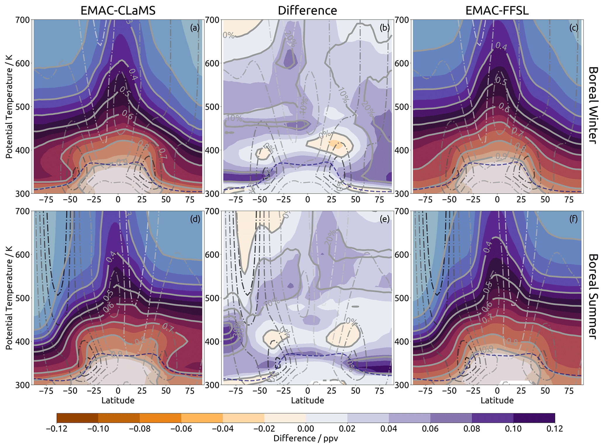
Figure 2Same as Fig. 1 but the quantity examined is a “forward-tracer” of 2-year lifetime (see text for details), with the exception that the percentage differences shown in (b) and (e) use EMAC-CLaMS as the baseline (i.e., 30 % means that EMAC-FFSL results show 30 % more forward tracer than those of EMAC-CLaMS).
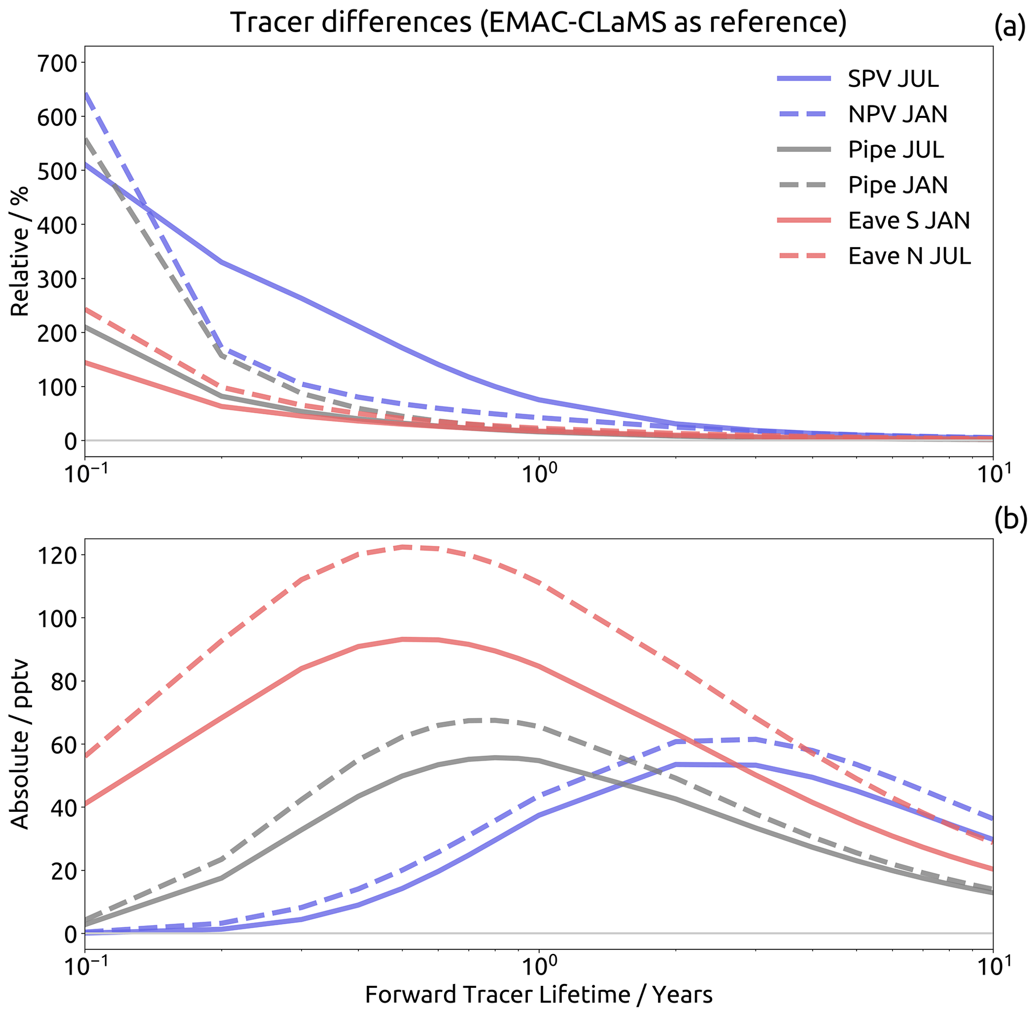
Figure 3Inter-representation difference (a relative difference, EMAC-FFSL minus EMAC-CLaMS normalized by EMAC-CLaMS; b: absolute difference, EMAC-FFSL minus EMAC-CLaMS) in forward tracer mixing ratios in several regions during January (“JAN”) and July (“JUL”), versus exponential decay lifetime of the tracer. Results are shown for the southern polar vortex (“SPV”, 70–90∘ S, 450 K), northern polar vortex (“NPV”, 70–90∘ S, 480 K), tropical pipe (“Pipe”, 5∘ S–5∘ N, 500 K), and summertime eave locations (“Eave”, 50∘–75∘ north or south, 360 K).
Figure 3 shows inter-representation differences in forward tracer mixing ratios at various locations for exponential decay lifetimes ranging from 1∕10 of a year to 10 years. In all locations and for all lifetimes, EMAC-FFSL shows larger tracer mixing ratios than EMAC-CLaMS, related to younger age in these regions (compare Fig. 1). The lifetime of the highest sensitivity to the transport scheme varies considerably between the different regions. In the lowermost stratosphere maximum differences occur for trace gas species with a lifetime of a few months (red lines). In the polar vortex, on the other hand, maximum differences occur for lifetimes of a few years (blues). Relative differences (in percent) show a different dependency on lifetime (monotonic decrease), as the tracer mixing ratio decreases with lifetime at a given location (Fig. 3). For short lifetimes, relative differences grow enormously in some regions. For instance in the polar vortex (both NH and SH) EMAC-FFSL tracer mixing ratios are higher than for EMAC-CLaMS by up to a factor of 5. The southern polar vortex stands out as a region with extremely large differences in the entire lifetime range below about 2 years.
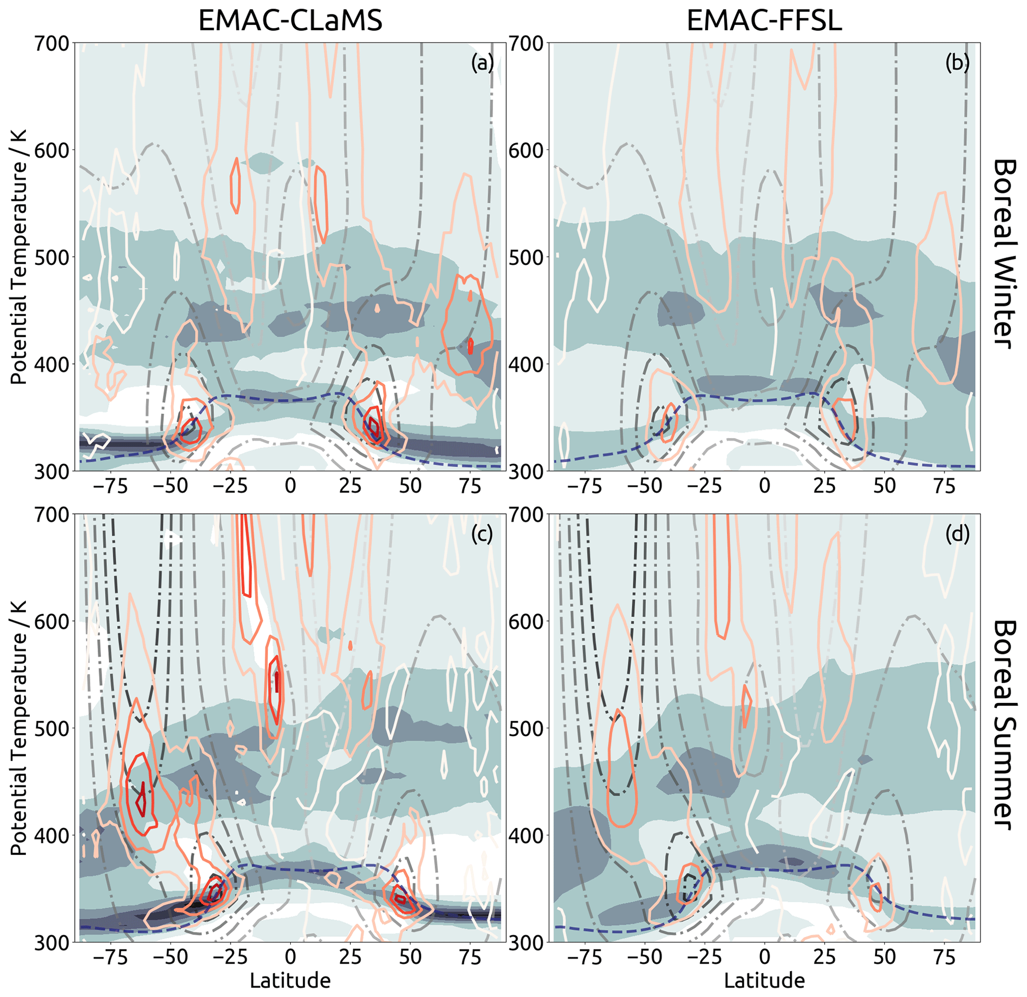
Figure 4Gradients of a 2-year lifetime forward tracer, from the tracer field calculated by the 10-year mean of representation age spectra. Shown are results from EMAC-CLaMS (a, c) and EMAC-FFSL (b, d) during January (a, b) and July (c, d). The vertical gradient is calculated with respect to potential temperature and shown in grey shading while the horizontal gradient is calculated with respect to the absolute value of latitude and shown with the colored line contours. Plotted gradients do not have explicit units; the vertical (horizontal) gradient is normalized to the maximum vertical (horizontal) gradient found in all four panels. Darker (redder) shading (contours) corresponds to the maximum value, while lighter (paler) shading (contours) corresponds to the smallest values. The steps between shadings (contours) are fixed fractions for both the filled and line contours.
Figure 4 presents horizontal and vertical gradients of the 2-year lifetime forward tracer. Broadly speaking, the vertical gradients are strongest along the tropopause, while the horizontal gradients are strongest at the subtropical jets, the polar vortexes (most strongly at the southern polar vortex), and the edges of the tropical pipe. While this is true in the results of both transport schemes, EMAC-CLaMS always shows gradients which are as strong or stronger than those of EMAC-FFSL. In particular, the vertical gradients at the extratropical tropopause are approximately twice as strong in EMAC-CLaMS, as are the horizontal gradients at the southern polar vortex and the edges of the tropical pipe. Meanwhile the horizontal gradients at the subtropical jets are approximately 50 % stronger in EMAC-CLaMS than in EMAC-FFSL. These results suggest that the representation of transport barriers is substantially stronger in EMAC-CLaMS than in EMAC-FFSL. While this has been shown for the case of the polar vortex already by Hoppe et al. (2014), the analysis here generalizes these findings to all the aforementioned stratospheric transport barriers.
3.3 Inter-annual variability
Inter-annual variability in the mean age fields is shown in Fig. 5. The results clearly indicate that the choice of transport scheme affects the simulated inter-annual transport variability. In both representations the greatest variability is found in the northern polar vortex and second to that at the edges of the tropical pipe. Whereas high mean age variability is found in the center of the northern polar vortex, for the southern polar vortex the strongest mean age variability is found at the edge of the vortex. This is the case in both schemes and is likely to be primarily related to the frequency of sudden stratospheric warmings, which occur much more often in the northern polar vortex than the southern polar vortex. In EMAC-FFSL, the mean age variability at the southern polar vortex edge is roughly equal to the variability found at the edges of the tropical pipe. However, in EMAC-CLaMS the variability at the edges of the tropical pipe is roughly twice as strong as the variability at the edge of the southern polar vortex. The inter-representation difference in this comparison is partially due to stronger southern polar vortex edge variability in EMAC-FFSL than EMAC-CLaMS. However, this discrepancy is smaller than the inter-representation difference in tropical pipe edge variability; variability at the tropical pipe edges is about twice as strong in EMAC-CLaMS as in EMAC-FFSL. This is also the case in the northern polar vortex, where mean age variability is about 50 % stronger in EMAC-CLaMS than in EMAC-FFSL.
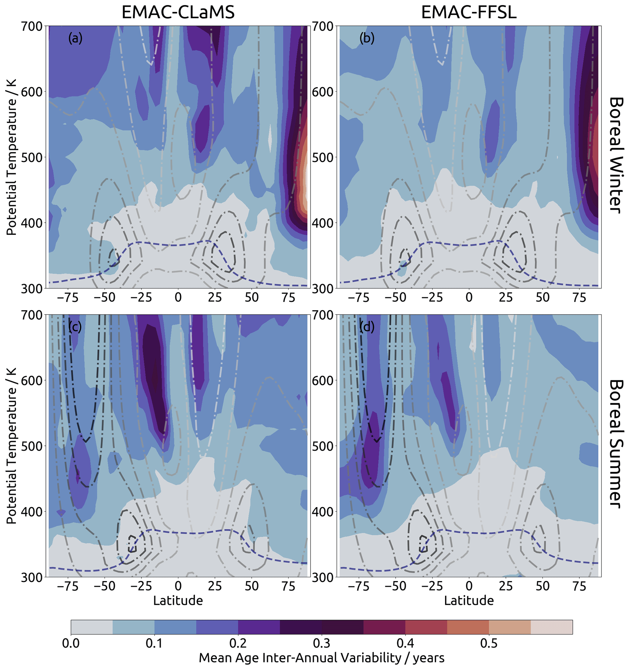
Figure 5Standard deviation of spectra monthly-average mean age over the 10-year climatology from EMAC-CLaMS (a, c) and EMAC-FFSL (b, d) during boreal winter (a, b) and summer (c, d).
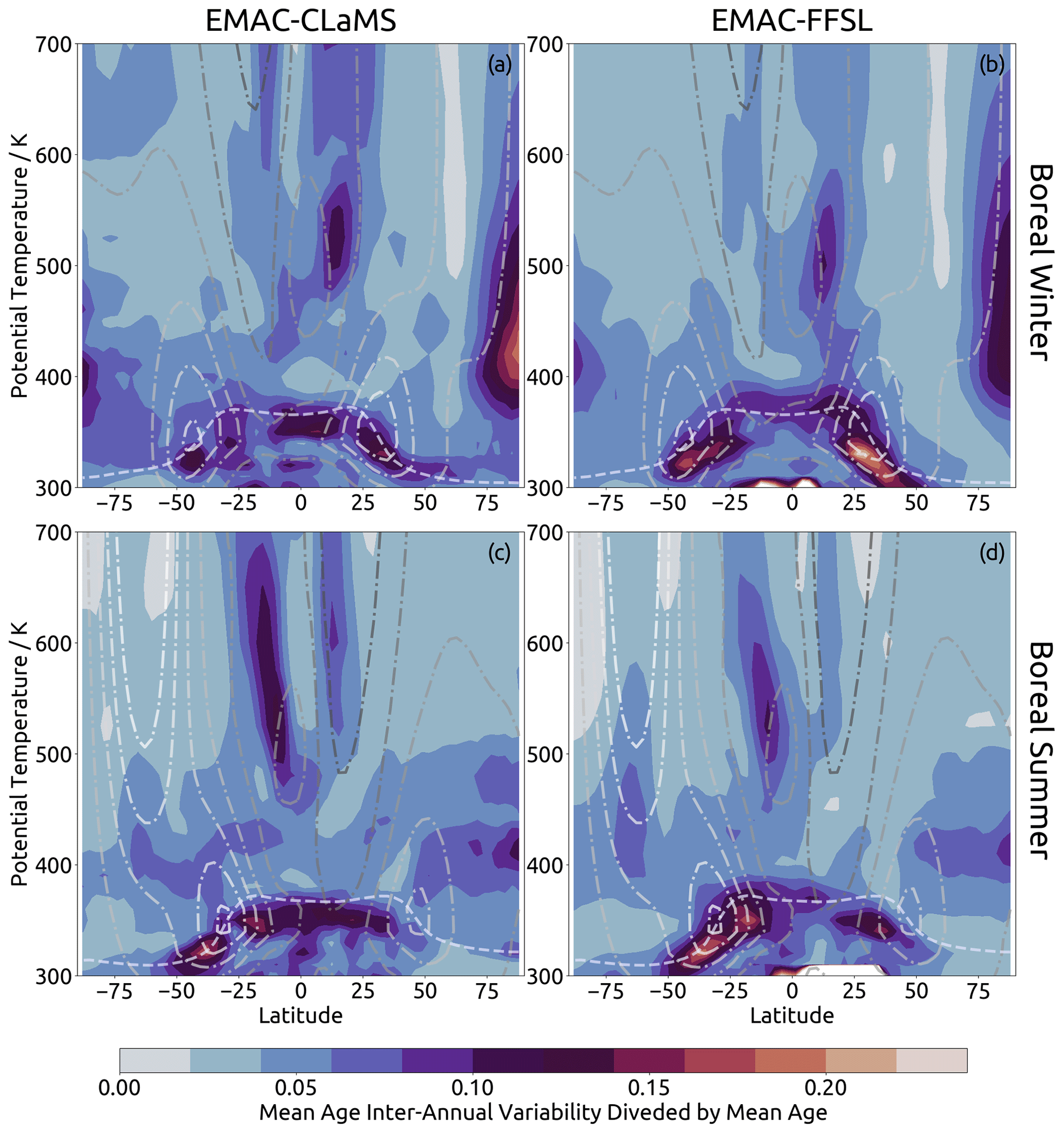
Figure 6Same as Fig. 5, but the quantity shown is the standard deviation of spectrum mean age scaled (divided) by the spectrum mean age.
Figure 6 shows inter-annual variability normalized by local mean age. From this perspective, the northern polar vortex still appears as a hotspot of variability and is still stronger in EMAC-CLaMS than in EMAC-FFSL. Conversely, the southern polar vortex edge shows much weaker variability compared to other locations, due to high mean age values in that region, and appears to have variability of approximately equal magnitude in both representations. The largest difference in this perspective from that of absolute difference values is found around the tropical tropopause. Variability in this location is stronger in EMAC-FFSL than in EMAC-CLaMS. Furthermore, in EMAC-FFSL this variability is strongest beyond the subtropical jets, rather than at the tropical tropopause (i.e., equatorward and upward of the subtropical jets). In the case of EMAC-CLaMS, variability beyond the subtropical jets is of a similar magnitude to variability along the tropical tropopause. These findings could indicate a critical role for transport across the subtropical jets to cause the differences in the eave structures in the age distribution between the Lagrangian and Eulerian frameworks (see Fig. 1). Analysis of the age spectra in Sect. 4.3 will shed more light on the reasons for the occurrence of the eaves.
3.4 Age spectrum shape
The age spectrum width is defined as the second moment of the spectra centered around the mean (e.g., Waugh and Hall, 2002)
The width quantifies the spread or dispersion of the spectra.
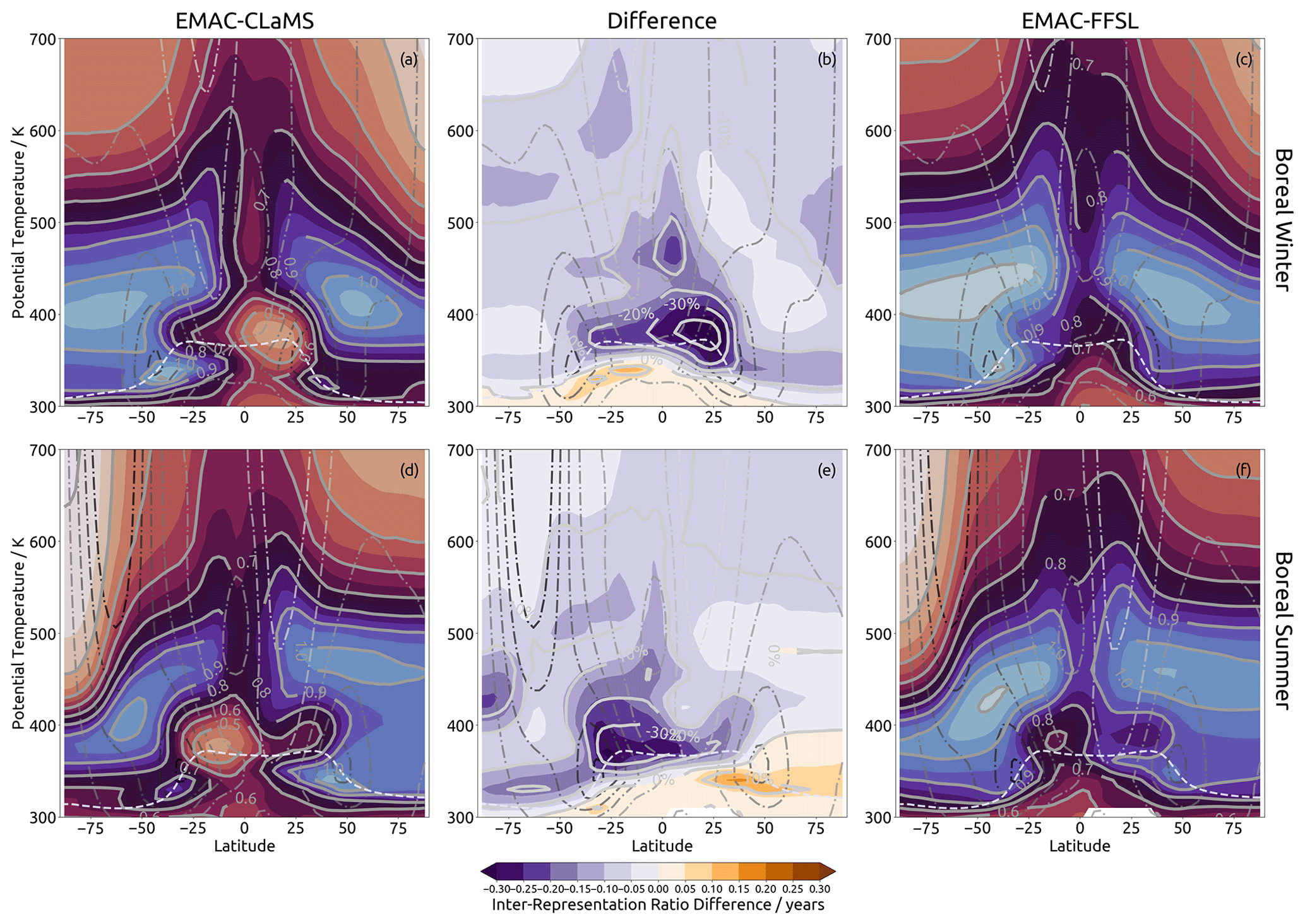
Figure 7Panels correspond to those of Fig. 2, but the quantity shown is the age spectra ratio of moments (width divided by mean age, units of years).
Spectrum width ranges from near zero to almost 2.5, with the lowest values found in the troposphere and the highest values found in the most troposphere-remote regions of the stratosphere, like the extratropical middle stratosphere and the polar vortexes (not shown). The summertime eave pattern in EMAC-CLaMS found in mean age and forward tracer contours is also seen in spectrum width as a region of higher widths (not shown).
An important parameter characterizing the shape of the age spectra is the “ratio of moments”, which we define as the spectrum width divided by the mean Δ2∕Γ. The ratio of moments is also a critical parameter for estimating mean age from trace gas measurements (e.g., Volk et al., 1997; Bönisch et al., 2009; Engel et al., 2009; Hauck et al., 2019, 2020), where the value is typically prescribed for the applied inverse method.
Figure 7 shows the ratio of moments from the age spectra. In general, the ratio of moments is relatively small in the tropics, related to narrow age spectra there, and increases in middle latitudes where age spectra are broader. The ratio of moments is larger in the summer compared to the winter hemisphere. The decrease at the upper levels and in the polar vortex is, to some degree, related to the truncation of the spectra at 10 years, which causes a slight underestimate of age spectrum width. The patterns agree qualitatively with results from other models (e.g., Hall and Plumb, 1994; Hauck et al., 2019). Quantitatively, the ratio values are lower than those found in the recent study by Hauck et al. (2019), which is related to the truncation of the spectrum tail here and should not be viewed as contrary to those results.
The inter-representation ratio differences (Fig. 7b and e) show that the ratio of moments (hence the spectrum shape) is sensitive to the transport scheme used. Throughout most regions of the stratosphere, the ratio of moments is larger in EMAC-FFSL than EMAC-CLaMS. The largest differences (up to 40 %) occur in the winter hemisphere subtropics at potential temperature levels between about 350 and 450 K. In this location, EMAC-CLaMS shows very localized region of low spectrum moment ratios, while EMAC-FFSL shows a much weaker minima and only shows this in the southern tropics.
The summertime lowermost stratosphere is the only region where the ratio of moments is larger in EMAC-CLaMS than EMAC-FFSL. A remarkable feature is the vertical dipole in the summertime subtropical lowest stratosphere with larger ratios below (around 350 K) smaller ratios (around 380 K). In other words, at this location relatively broad spectra reside below narrower spectra. This characteristic in the ratio of moments is much more clear in EMAC-CLaMS than in EMAC-FFSL and is likely related to the eave structures found in the mean age distribution in EMAC-CLaMS. The details of the age spectra in this region will be investigated in Sect. 4.3.
To gain further insight into inter-representation differences in transport processes, we turn our investigation to the stratospheric age spectrum. This section is subdivided according to the regions with the most significant differences: the tropical and mid-latitude stratosphere, the polar vortexes, and the lowermost stratosphere.
4.1 Tropical and mid-latitude stratosphere
Air enters the stratosphere across the tropical tropopause in the TTL and is then transported upwards in the tropical pipe by the deep branch or poleward by the shallow branch of the BDC (Brewer–Dobson circulation). Within the tropical pipe, with its lower edge at about 450 K, exchange with middle latitudes is suppressed and air is thereby largely confined therein (Plumb, 1996).
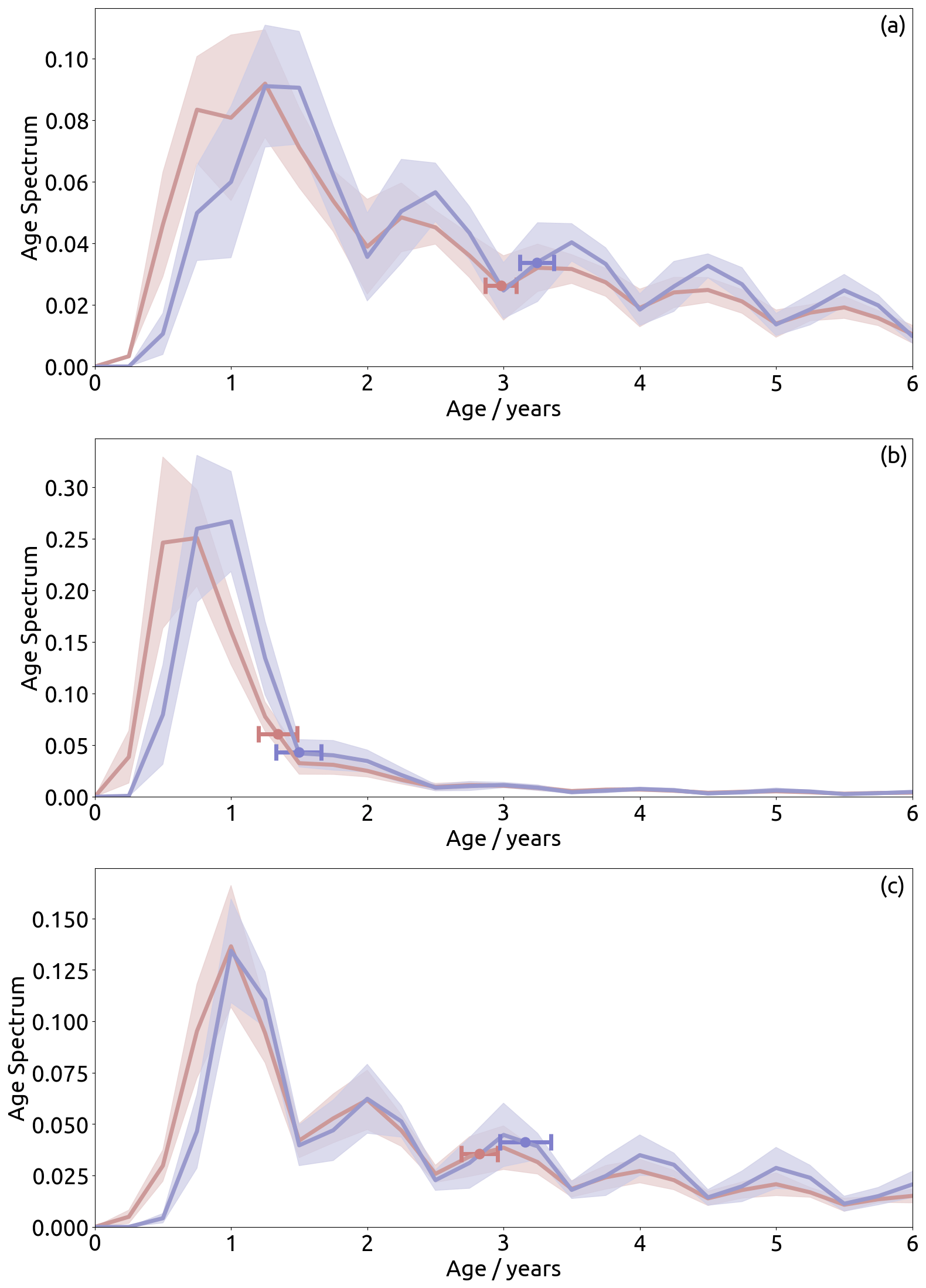
Figure 8Age spectra from the results of EMAC-FFSL (red) and EMAC-CLaMS (blue) at 500 K for (a) the southern mid-latitude stratosphere (40–60∘ S, July), (b) the tropical pipe (6∘ S–6∘ N, January), and (c) the northern mid-latitude stratosphere (40–60∘ N, January). Lines indicate multi-annual mean, with shading showing annual variability. Dots indicate mean age of spectra, with surrounding bars showing annual variability. Variability for both quantities is computed as 2 standard deviations.
Figure 8b shows age spectra from EMAC-FFSL and EMAC-CLaMS at the 500 K level during boreal winter (January) in the tropical pipe. Results during boreal summer are very similar (not shown). There is a clear shift of the EMAC-FFSL spectrum (red) towards younger ages for the transit time range below about 2 years, compared to EMAC-CLaMS. This shift shows a higher fraction of air younger than 9 months in EMAC-FFSL, resulting from much faster tropical upward transport from that transport scheme. For a transit time of 3 months (which is the age spectrum resolution; see Sect. 2), EMAC-FFSL shows a substantial air mass fraction of about 4 %, whereas in EMAC-CLaMS there is no such air. Results for the next transit time bin (at 6 months) are similar: the EMAC-FFSL air mass fraction is significantly larger than for EMAC-CLaMS (about 0.25 compared to 0.075). As 3 months is beyond the fastest transit time from the middle troposphere to 500 K based on large-scale upwelling velocities (Wright and Fueglistaler, 2013), the differences at short transit times can only be caused by stronger vertical diffusion due to numerical diffusion in the FFSL transport scheme.
Comparison of age spectra in northern middle latitudes at the same level (Fig. 8c) shows smaller differences and even the same modal age (defined as the transit time at the age spectrum peak) for EMAC-FFSL and EMAC-CLaMS. However, in this case EMAC-FFSL transport again clearly shows a larger fraction of young air with transit times less than a year. Similar to the case of tropical transport these differences must be related to stronger numerical diffusion in the EMAC-FFSL transport scheme. Another interesting feature is the stronger multiple peaks in the spectrum tail for EMAC-CLaMS (from ages of 3 years above). The occurrence of multiple peaks in stratospheric age spectra is caused by the seasonality of transport into the stratosphere (Reithmeier and Sausen, 2008; Ploeger and Birner, 2016). Stronger numerical diffusion in EMAC-FFSL blurs this seasonal transport signal over the course of a few years.
Very similar conclusions hold for the Southern Hemisphere middle latitudes during austral winter (Fig. 8a). The fraction of young air (age below about 1 year) here is greater in EMAC-FFSL compared to EMAC-CLaMS, related to stronger diffusion of the transport scheme, and the peaks in the spectrum tail are again weaker.
4.2 Polar vortex
Due to strong polar downwelling motion and the cyclonic circumpolar flow, air masses inside the wintertime stratospheric polar vortexes are largely isolated against exchange with middle latitudes, even more so in the Southern Hemisphere, where the cyclonic circumpolar flow is stronger than in the Northern Hemisphere. Figure 9b shows the age spectra within the southern stratospheric polar vortex. Below 3 years, the spectra show clear qualitative differences. EMAC-FFSL shows two peaks in this region: one at 2.5 years and the other at 1.25 years. Meanwhile EMAC-CLaMS shows only one peak, which is at 2.5 years. The common peak at 2.5 years is much stronger in EMAC-CLaMS than in EMAC-FFSL. The contribution from air younger than 2 years is about twice as strong in EMAC-FFSL as in EMAC-CLaMS. This much higher fraction of young air inside the polar vortex in EMAC-FFSL than in EMAC-CLaMS is caused by stronger diffusive transport across the vortex edge in the FFSL transport scheme. This difference suggests that simulations of chemically active tracers with short stratospheric lifetimes and tropospheric origins would show substantially stronger southern polar vortex concentrations in EMAC-FFSL, compared to EMAC-CLaMS. For long-lived trace gas species differences would be smaller. Consequently, the amount of ozone-depleting substances in polar regions with lifetimes below a few years and related polar ozone loss can substantially differ depending on the chosen transport scheme.
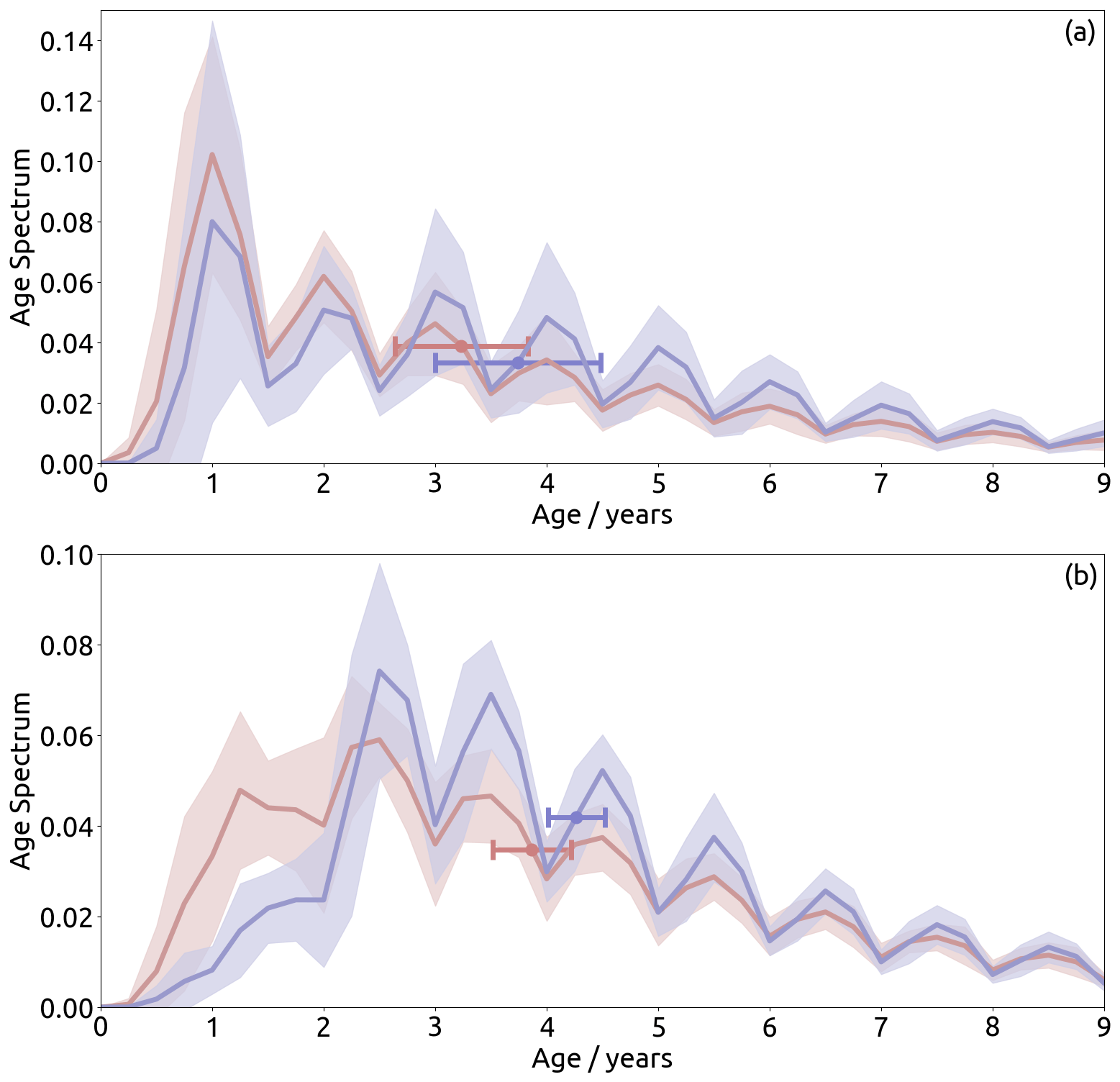
Figure 9Age spectra from EMAC-FFSL (red) and EMAC-CLaMS (blue) within (a) the northern polar vortex (480 K, 70–90∘ N, January) and (b) the southern polar vortex (90–70∘ S 450 K, July). Lines indicate multi-annual mean with shading showing annual variability. Dots indicate mean age of spectra, with surrounding bars showing annual variability. Variability for both quantities is computed as 2 standard deviations.
Variability in the age spectra seems to be roughly similar at most ages but is substantially different below 3 years of age, with much more variability in EMAC-CLaMS at the 2.5-year peak and much more variability in EMAC-FFSL below 2 years of age. At ages older than 3 years, the age spectra are qualitatively similar, showing multiple maxima at 1-year intervals at the half-year marks and regular minima at the 1-year marks. This means stronger contribution of air emitted during January and weaker contribution of air emitted during July. Both schemes show this quality, with EMAC-CLaMS showing a greater difference between the contributions at the maxima and minima.
Figure 9a shows age spectra within the northern polar vortex. As in the southern polar vortex, ages above 3 years show qualitative similarity between the representations; maxima in the spectra correspond to January-emitted tracers while minima correspond to July-emitted tracers. At ages younger than 2.75 years, EMAC-FFSL shows greater tracer concentrations than EMAC-CLaMS. However, the difference between the two representations in this location for young ages is much smaller than the difference in the southern polar vortex, while variability in the age spectra is much stronger (approximately a factor of 2) in EMAC-CLaMS than in EMAC-FFSL.
4.3 Lowermost stratosphere
A particularly interesting feature in the mean age and tracer distributions in the summertime lowermost stratosphere in Figs. 1 and 2 is the eave structure. The structure – only found in EMAC-CLaMS – has two features: an old-air region at the level of the subtropical jet (around 360 K) and a young-air region above that (around 400 K). Conversely, in EMAC-FFSL these two regions have a similar age. As the mean age and forward tracer contours in Figs. 1 and 2 in the upper region follow similar paths in both representations, transport from the upper region into the lower region is not likely to play a role in the discrepancy of the eave structure representation. Therefore, the eave structure, as present in EMAC-CLaMS, probably arises from weaker direct transport from the troposphere (i.e., not through the tropical tropopause layer) into the lower eave region, in comparison to EMAC-FFSL.
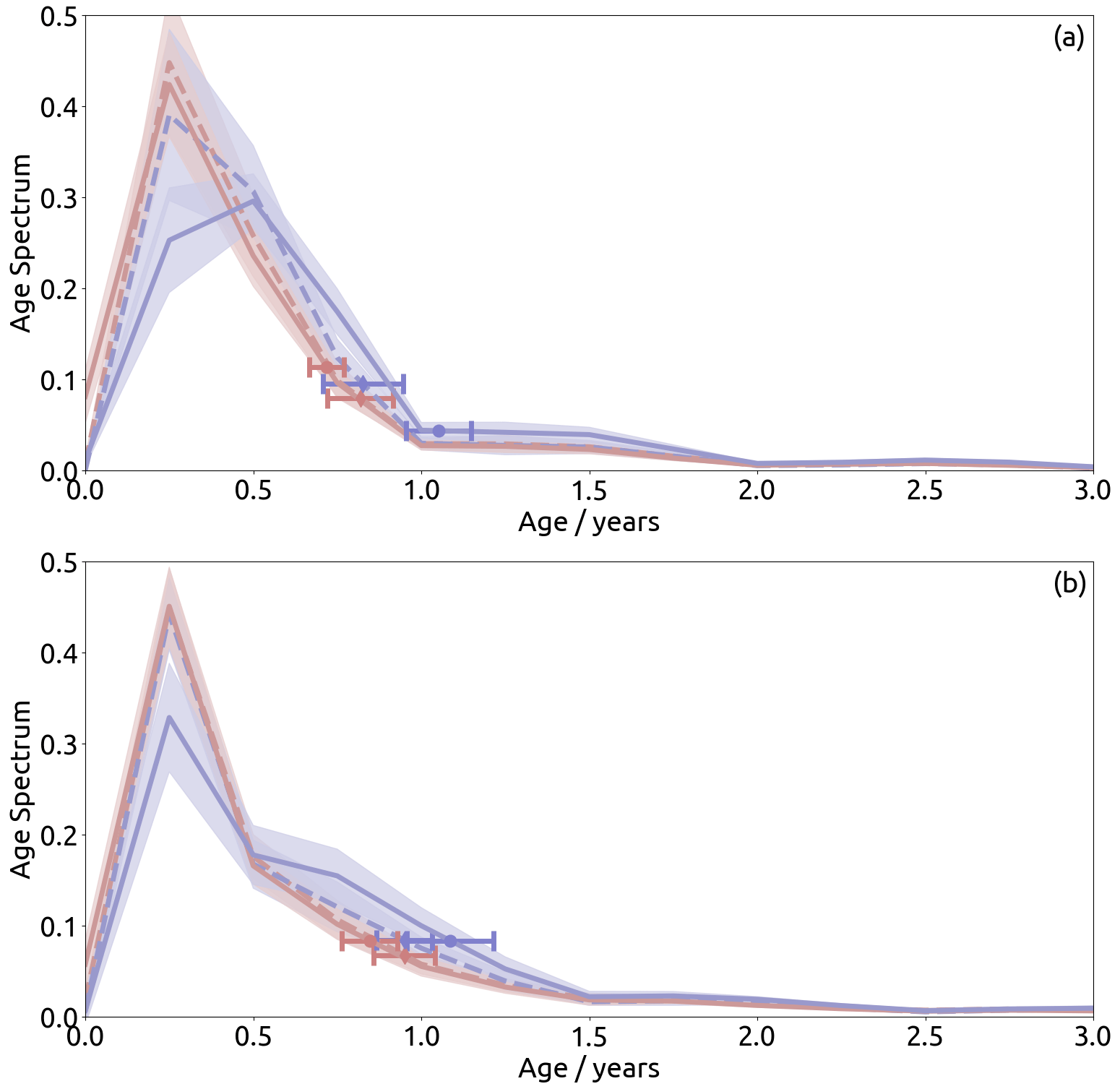
Figure 10Age spectra from the results of EMAC-FFSL (red) and EMAC-CLaMS (blue) within the summertime lowermost stratosphere regions of the eave structures at 360 K (sold lines) and 400 K (dashed lines) in (a) the Northern Hemisphere (55–75∘ N, July) and (b) the Southern Hemisphere (55–75∘ S, January).
To gain more insight into the underlying processes, Fig. 10 shows the corresponding age spectra for the two schemes at the 360 and 400 K levels between 50–60∘ latitude. In both cases, the upper-level age spectra are very similar in both EMAC-FFSL and EMAC-CLaMS. In the Southern Hemisphere in particular, these spectra are nearly identical, with only slightly more tracer between 0.5 and 1.5 years of age found in EMAC-CLaMS. Meanwhile the Northern Hemisphere results show somewhat less agreement between the two representations in the upper levels, with slightly less tracer at 0.25 years and somewhat more tracer between 0.5 and 1.0 years in EMAC-CLaMS. However, there is considerable inter-representation difference in the relationship between the age spectra in the upper region and the lower region; EMAC-FFSL results show nearly identical spectra in both regions, while EMAC-CLaMS shows a consistent difference in the upper and lower region spectra. In the EMAC-CLaMS spectra for both hemispheres, the upper region shows more air younger than 0.5 years while the lower region shows more air between 0.5 years and 1.5 years, and both regions show nearly identical contributions from air at 0.5 years.
The differences in age spectra, mean age, and tracer mixing ratios suggest that the eave structure in the lowermost stratosphere is caused by an interplay of transport processes as described in the following. The lowermost stratosphere mean age distribution results from a mixture of old air masses downwelling from the stratosphere and young air masses transported into the region by the shallow branch of the BDC (e.g., Bönisch et al., 2009). In spring and summer, a new transport pathway emerges which is related to upward transport in the tropics and poleward transport directly above the subtropical jet, and it is characterized by transport timescales of about half a year to 1.5 years. This poleward transport happens in the layer of about 380–450 K, which belongs to the region above the subtropical jet and below the tropical pipe. Fast transport in this layer agrees well with the existence of a tropically controlled transition region for water vapor as proposed by Rosenlof et al. (1997). The EMAC-CLaMS simulation shows a clear age inversion related to this flushing of the extratropical lowermost stratosphere with young air above the jet. In the EMAC-FFSL simulation, on the other hand, this feature is totally absent because a much higher fraction of young air with transit times shorter than 0.5 years blurs the old-air signature in the layer around 350 K.
Hence, the Lagrangian and Eulerian transport schemes result in different preferences for transport pathways into the summertime lowermost stratosphere: poleward transport above the jet (Lagrangian) versus cross-tropopause transport at levels below (Eulerian). It remains to be shown from trace gas observations in the lowermost stratosphere whether the eave structure evident in the age distribution from Lagrangian transport is a feature of the observed atmosphere. Initial indications for a mixture of old wintertime air and young air masses from transport above the subtropical jet in that region during early spring have already been found in aircraft in situ measurements of N2O and CO by Krause et al. (2018).
The results of the work presented thus far have shown substantial differences in tracer transport between EMAC-FFSL and EMAC-CLaMS. Given that the FFSL transport scheme used by EMAC is also used in a wide array of other climate models, the effects of unphysical numerical diffusion in EMAC-FFSL which have been described here are likely to affect tracer transport in other climate models as well. This could cause complications for the interpretation of results from these models, especially for stratospheric transport. One such topic, for which there is considerable modeling activity at the moment, is geoengineering through stratospheric aerosol injection (SAI). This has been proposed as a method to reduce or entirely offset the surface temperature effects of global warming (e.g., Crutzen, 2006) and is likely to gather more attention as the global mixing ratios of greenhouse gases rise. Relatedly, the latest-generation climate models from the Coupled Model Intercomparison Project Phase 6 (CMIP6) show an even stronger equilibrium climate sensitivity and simulate stronger climate warming than the model generation before (Forster et al., 2020), further fueling discussion about solar geoengineering.
A modeling effort to assess the opportunities and risks of solar geoengineering using stratospheric sulfate aerosols within the Geoengineering Large Ensemble (GLENS) project has recently been presented by Tilmes et al. (2018). In this project, injection strategies have been proposed to maintain the distribution of global surface temperatures in the future, and potential side effects (e.g., on precipitation and stratospheric ozone) have been discussed (Kravitz and Douglas, 2020). Although the results of that work suggest that it may be possible to use SAI successfully (i.e., to maintain the global distribution of surface temperatures), the authors note that a main uncertainty in their model results is related to stratospheric transport processes and their representation in current climate models.
Our model experiment, which applies one climate model with two different transport schemes in the same simulation, is well-suited to shed further light on this uncertainty of geoengineering projections related to uncertainties in air mass dispersal due to the model representation of stratospheric transport. It is noteworthy here that this discussion concerns air mass transport and not the transport of sulfate, as our simulation does not include stratospheric chemistry. However, we consider a state-of-the-art transport scheme (EMAC-FFSL) which is also applied in other current climate models and a novel Lagrangian scheme (EMAC-CLaMS) which has significantly less numerical diffusion. As results from this paper show, two regions emerge where transport differences between the two representations are especially large: the lowermost stratosphere and the polar vortex. Both are critical regions for the processes which affect the efficacy of SAI. In particular, sulfate concentrations in the lowermost stratosphere crucially affect radiative forcing, whereas sulfate concentrations in the polar vortex control the side effects of geoengineering on stratospheric ozone.
Figure 11Region from the plume injection experiment showing results for a long-lived (365 d lifetime) tracer. (a) EMAC-FFSL results on the EMAC grid at model level 63 (approximately 100 hPa, and the level at which plume injection occurred). (b) EMAC-CLaMS results gridded onto the EMAC model grid at the same level as the EMAC results. (c) EMAC-CLaMS data for parcels within EMAC model level 63 in the unprocessed Lagrangian representation. (d) Histograms showing distributions of tracer mixing ratios within the shown region. The color map used in (a–c) corresponds to the background colors in (d). Histograms are shown for unprocessed EMAC-CLaMS results (solid line, corresponding to distribution in c), EMAC-CLaMS gridded results (long-dashed line, corresponding to distribution in b), and EMAC-FFSL results (short-dashed line, corresponding to distribution in a). Histograms are computed using only data which are shown in the other three panels (i.e., within the shown region and within EMAC model level 63), and the histograms of gridded results are mass-weighted.
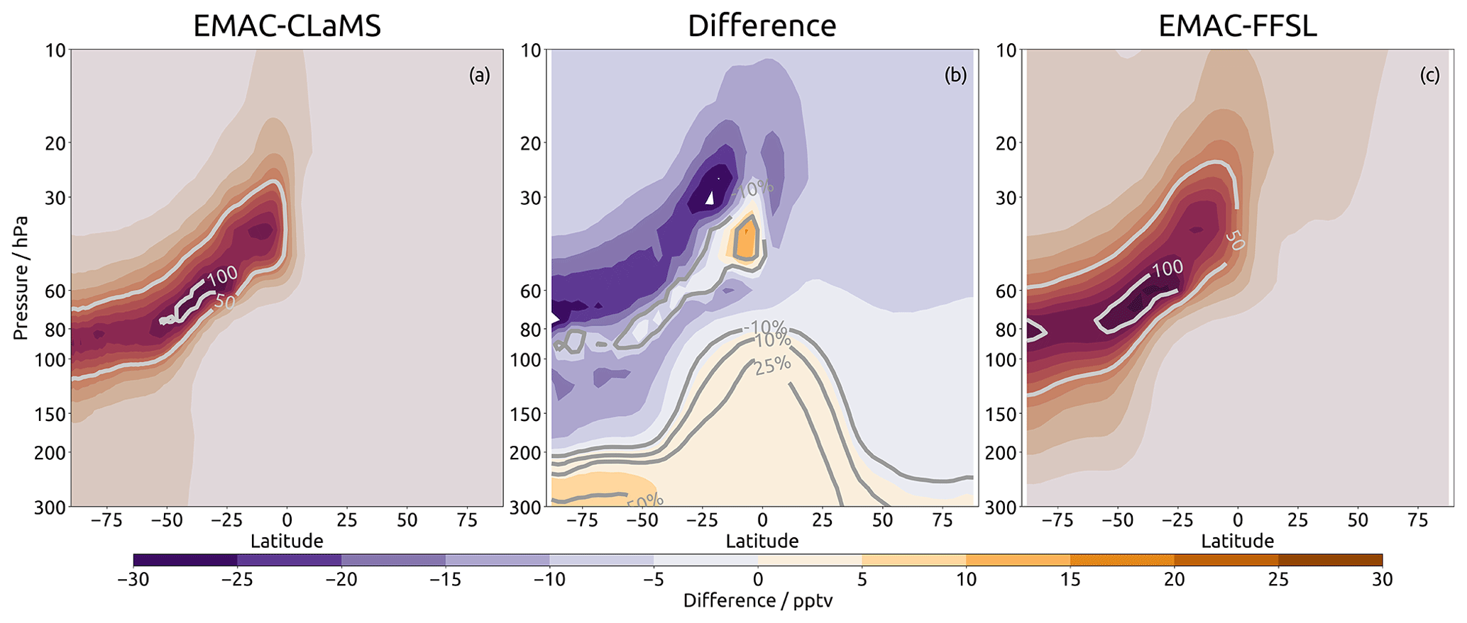
Figure 12Zonal mean tracer distribution from continuous mass injection in the stratosphere (30∘ S, 100 hPa) from EMAC-CLaMS (a) and EMAC-FFSL (c) results, contours showing tracer mixing ratios in parts per trillion by volume (emission value of 1 ppbv). Also shown is the difference between the fields (b) with both absolute differences (shading) and percentage differences (contours, EMAC-CLaMS as reference). Results are shown for a 1-year lifetime tracer.
To illustrate the potential differences in geoengineering simulations caused by model transport representation, we modified our experiments to include continuous point-source injections of tracers with idealized chemistry. The injection is handled by forcing the tracer mixing ratio to 1 ppbv within a region of nine EMAC grid cells (three cells wide both east–west and north–south). The idealized chemistry is represented by a global exponential decrease with 30, 90, and 365 d lifetimes. Figure 11 shows the dispersal of a 365 d lifetime tracer which was injected at 30∘ N and 180∘ E at the 89 hPa pressure level. The results are shown for the two transport schemes after about 5 years of simulation and the results represent the state of the simulation on a single time step. Both models show three regions with high tracer mixing ratios: (1) a plume between 300 and 330∘ E which is the most prominent feature of the snapshot, (2) a second plume west of 260E and between 40–50∘ S, (3) and then a third local maxima of tracer mixing ratios in the upper northwest corner of the image. In the EMAC-FFSL results, this latter region seems to be separate from the others in the image, while in EMAC-CLaMS this region seems to be connected to the main plume by a trail of weaker tracer mixing ratios. In both features (1) and (2), EMAC-CLaMS results show higher mixing ratios in the centers of the plumes. In feature (1), these mixing ratios even reach nearly as high as the emission mixing ratio (1 ppbv), showing that the central area of the plume remained isolated during transport over 60∘ of longitude. In comparison, the highest mixing ratios found in EMAC-FFSL are about 0.45 ppbv – half the emission mixing ratio. Furthermore, there is clearly a much wider variety of small-scale features in the results of EMAC-CLaMS compared to those from EMAC. Hence, the stronger numerical diffusion in EMAC's FFSL transport scheme blurs small-scale features and filaments compared to Lagrangian transport and results in a more homogeneous tracer distribution.
Global tracer distributions from the two models at the end of the 5-year simulation period (for the 365 d lifetime tracer) are shown in Fig. 12 for the case of austral spring (September–November). The tracer plume extending from the injection source location in the southern subtropics towards the south pole is broader and more smeared out in EMAC-FFSL than EMAC-CLaMS, also related to the differences in numerical diffusion. The difference figure (Fig. 12) indicates even clearer that for EMAC-CLaMS the plume is more centered around its core whereas for EMAC-FFSL it is broader with more tracer above and below. In particular inside the polar vortex (poleward of about 60∘ S), tracer mixing ratios are substantially (approximately 35 %) higher for the more diffusive FFSL transport scheme.
These differences emerge for all injected tracers considered, including over each of the lifetimes of 30, 90, and 365 d. We therefore expect that for realistic chemistry there should also be significantly higher sulfur concentrations in polar regions for more diffusive model transport schemes, compared to Lagrangian schemes. As relative differences in the polar vortex are substantial, we expect a large uncertainty of simulated ozone depletion from geoengineering sulfur injections related to the used model transport scheme. Narrowing this uncertainty further down, in particular using simulations including appropriate stratospheric chemistry for sulfur and ozone, should be a priority for future research in this direction. For the moment, in view of such large uncertainties in stratospheric transport in current models and the potential dangers of SAI geoengineering, real-world applications of SAI remain highly questionable and inadvisable.
In this work, we have assessed the impact of the choice of trace gas transport scheme on the representation of stratospheric transport. The two transport schemes that we have studied are the Lagrangian scheme of CLaMS and the Eulerian FFSL scheme of EMAC, the latter of which is commonly used in modern chemistry–climate models. Differences in transport timescales were investigated by comparing the full time-dependent age spectrum and idealized, radioactively decaying forward tracers in representations from both schemes. The results show that stratospheric transport barriers are, in general, much stronger in simulations with Lagrangian trace gas transport whereas they are weaker for the FFSL scheme due to stronger, unphysical numerical diffusion associated with the latter method. These results are broadly consistent with previous studies comparing Lagrangian and Eulerian transport, in particular the works of Hoppe et al. (2014, 2016) and Stenke et al. (2008, 2009), both of which found slower transport and stronger transport barriers in Lagrangian schemes. These conclusions hold for the transport barriers around the polar vortex, along the subtropical jets, and at the edges of the tropical pipe. Two regions of the stratosphere emerge from the simulations for which differences caused by the transport scheme are particularly large: (i) the polar vortex and (ii) the summertime lowermost stratosphere. Inside the polar vortex, the air is substantially older in the Lagrangian transport simulation due to reduced diffusive transport from middle latitudes through the vortex edge. Consequently, chemical tracers with short lifetimes show much lower mixing ratios. Also in the lowermost stratosphere, the air is much older for the Lagrangian simulation, as diffusive cross-tropopause transport of young air from the troposphere is reduced.
In particular, a very different structure in the age of air and tracer distributions emerges in the summertime lowermost stratosphere in the two representations. The Lagrangian representation of EMAC-CLaMS shows an age inversion structure, or eave, where older air resides below younger air, while this feature is entirely absent in the EMAC-FFSL results. This structure is related to fast poleward transport above the jet, which creates the young air layer above the older air. In the EMAC-FFSL results, strong diffusive cross-tropopause transport totally blurs this layered structure.
The results of this paper show that a fully Lagrangian transport scheme (that of CLaMS) results in significantly less numerical diffusion, stronger stratospheric transport barriers, and clearer structures in trace gas distributions (e.g., gradients, filaments), even when compared to a sophisticated, state-of-the-art flux-form semi-Lagrangian scheme (that of EMAC). Differences in simulated trace gas transport related to the choice of the transport scheme raise important questions about the uncertainty of stratospheric transport in climate model simulation and in particular for geoengineering model experiments.
The model code used in this work is a part of the MESSy project and is available to all persons who agree to the MESSy terms of use. Information on obtaining this permission can be found at messy-interface.org. Interested persons are also welcome to contact the corresponding author (Edward.Charlesworth.ScienceGMail.com).
EJC and FP prepared the manuscript of this work with assistance from all other authors. Model development was performed by EJC, FF, and PJ. Simulations were executed by EJC and AKD. All authors contributed to analysis and interpretation of results.
The authors declare no competing interests.
We would like to thank Nicole Thomas for her invaluable technical assistance as well as Hella Garny, Marius Hauck, and Peter Hoor, with whom we had very stimulating discussions. Finally, we gratefully acknowledge the computing time for the EMAC simulations which was granted on the supercomputer JURECA at the Jülich Supercomputing Centre (JSC) under the VSR project ID JICG11.
This work was funded by the Helmholtz Association under grant no. VH-NG-1128 (Helmholtz Young Investigators Group A-SPECi) and was also enabled by the Helmholtz Association Earth System Modeling project.
The article processing charges for this open-access
publication were covered by a Research
Centre of the Helmholtz Association.
This paper was edited by Jianzhong Ma and reviewed by three anonymous referees.
Abalos, M., Legras, B., and Shuckburgh, E.: Interannual variability in effective diffusivity in the upper troposphere/lower stratosphere from reanalysis data, Q. J. Roy. Meteor. Soc., 142, 1847–1861, https://doi.org/10.1002/qj.2779, 2016. a
Abalos, M., Randel, W. J., Kinnison, D. E., and Garcia, R. R.: Using the Artificial Tracer e90 to Examine Present and Future UTLS Tracer Transport in WACCM, J. Atmos. Sci., 74, 3383–3403, https://doi.org/10.1175/JAS-D-17-0135.1, 2017. a
Bönisch, H., Engel, A., Curtius, J., Birner, Th., and Hoor, P.: Quantifying transport into the lowermost stratosphere using simultaneous in-situ measurements of SF6 and CO2, Atmos. Chem. Phys., 9, 5905–5919, https://doi.org/10.5194/acp-9-5905-2009, 2009. a, b
Brinkop, S. and Jöckel, P.: ATTILA 4.0: Lagrangian advective and convective transport of passive tracers within the ECHAM5/MESSy (2.53.0) chemistry–climate model, Geosci. Model Dev., 12, 1991–2008, https://doi.org/10.5194/gmd-12-1991-2019, 2019. a
Butchart, N.: The Brewer-Dobson circulation, Rev. Geophys., 52, 157–184, https://doi.org/10.1002/2013RG000448, 2014. a
Butler, A. H., Sjoberg, J. P., Seidel, D. J., and Rosenlof, K. H.: A sudden stratospheric warming compendium, Earth Syst. Sci. Data, 9, 63–76, https://doi.org/10.5194/essd-9-63-2017, 2017. a
Crutzen, P. J.: Albedo enhancements by stratospheric sulfur injections: a contribution to resolve a policy dilemma? An Editorial Essay, Clim. Change, 77, 211–219, 2006. a
Diallo, M., Legras, B., and Chédin, A.: Age of stratospheric air in the ERA-Interim, Atmos. Chem. Phys., 12, 12133–12154, https://doi.org/10.5194/acp-12-12133-2012, 2012. a
Eluszkiewicz, J., Hemler, R. S., Mahlman, J. D., Bruhwiler, L., and Takacs, L. L.: Sensitivity of Age-of-Air Calculations to the Choice of Advection Scheme, J. Atmos. Sci., 57, 3185–3201, https://doi.org/10.1175/1520-0469(2000)057<3185:SOAOAC>2.0.CO;2, 2000. a
Engel, A., Möbius, T., Bönisch, H., Schmidt, U., Heinz, R., Levin, I., Atlas, E., Aoki, S., Nakazawa, T., Sugawara, S., Moore, F., Hurst, D., Elkins, J., Schauffler, S., Andrews, A., and Boering, K.: Age of stratospheric air unchanged within uncertainties over the past 30 years, Nat. Geosci., 2, 28–31, https://doi.org/10.1038/ngeo388, 2009. a
Forster, P. M., Maycock, A. C., McKenna, C. M., and Smith, C. J.: Latest climate models confirm need for urgent mitigation, Nat. Clim. Change, 10, 7–10, https://doi.org/10.1038/s41558-019-0660-0, 2020. a
Fritsch, F., Garny, H., Engel, A., Bönisch, H., and Eichinger, R.: Sensitivity of age of air trends to the derivation method for non-linear increasing inert SF6, Atmos. Chem. Phys., 20, 8709–8725, https://doi.org/10.5194/acp-20-8709-2020, 2020. a
Fueglistaler, S., Dessler, A. E., Dunkerton, T. J., Folkins, I., Fu, Q., and Mote, P. W.: Tropical tropopause layer, Rev. Geophys., 47, RG1004, https://doi.org/10.1029/2008RG000267, 2009. a, b
Gregory, A. R. and West, V.: The sensitivity of a model's stratospheric tape recorder to the choice of advection scheme, Q. J. Roy. Meteorol. Soc., 1, 64–75, https://doi.org/10.1038/s43017-019-0004-7, 2002. a
Gupta, A., Gerber, E. P., and Lauritzen, P. H.: Numerical impacts on tracer transport: A proposed intercomparison test of Atmospheric General Circulation Models, Q. J. Roy. Meteor. Soc., 3937–3964, https://doi.org/10.1002/qj.3881, 2020. a
Hall, T. M. and Plumb, R. A.: Age as a diagnostic of stratospheric transport, J. Geophys. Res., 99, 1059–1070, 1994. a
Hall, T. M., Waugh, D. W., Boering, K. A., and Plumb, R. A.: Evaluation of transport in stratospheric models, J. Geophys. Res.-Atmos., 104, 18815–18839, https://doi.org/10.1029/1999JD900226, 1999. a
Hauck, M., Fritsch, F., Garny, H., and Engel, A.: Deriving stratospheric age of air spectra using an idealized set of chemically active trace gases, Atmos. Chem. Phys., 19, 5269–5291, https://doi.org/10.5194/acp-19-5269-2019, 2019. a, b, c, d, e, f
Hauck, M., Bönisch, H., Hoor, P., Keber, T., Ploeger, F., Schuck, T. J., and Engel, A.: A convolution of observational and model data to estimate age of air spectra in the northern hemispheric lower stratosphere, Atmos. Chem. Phys., 20, 8763–8785, https://doi.org/10.5194/acp-20-8763-2020, 2020. a
Haynes, P. and Shuckburgh, E.: Effective diffusivity as a diagnostic of atmospheric transport: 1. Stratosphere, J. Geophys. Res.-Atmos., 105, 22777–22794, https://doi.org/10.1029/2000JD900093, 2000. a
Holton, J. R., Haynes, P., McIntyre, M. E., Douglass, A. R., Rood, R. B., and Pfister, L.: Stratosphere-troposphere exchange, Rev. Geophys., 33, 403–439, 1995. a, b
Hoppe, C. M., Hoffmann, L., Konopka, P., Grooß, J.-U., Ploeger, F., Günther, G., Jöckel, P., and Müller, R.: The implementation of the CLaMS Lagrangian transport core into the chemistry climate model EMAC 2.40.1: application on age of air and transport of long-lived trace species, Geosci. Model Dev., 7, 2639–2651, https://doi.org/10.5194/gmd-7-2639-2014, 2014. a, b, c, d, e, f, g, h, i
Hoppe, C. M., Ploeger, F., Konopka, P., and Müller, R.: Kinematic and diabatic vertical velocity climatologies from a chemistry climate model, Atmos. Chem. Phys., 16, 6223–6239, https://doi.org/10.5194/acp-16-6223-2016, 2016. a, b
Jöckel, P., Sander, R., Kerkweg, A., Tost, H., and Lelieveld, J.: Technical Note: The Modular Earth Submodel System (MESSy) – a new approach towards Earth System Modeling, Atmos. Chem. Phys., 5, 433–444, https://doi.org/10.5194/acp-5-433-2005, 2005. a
Jöckel, P., Kerkweg, A., Pozzer, A., Sander, R., Tost, H., Riede, H., Baumgaertner, A., Gromov, S., and Kern, B.: Development cycle 2 of the Modular Earth Submodel System (MESSy2), Geosci. Model Dev., 3, 717–752, https://doi.org/10.5194/gmd-3-717-2010, 2010. a
Jöckel, P., Tost, H., Pozzer, A., Kunze, M., Kirner, O., Brenninkmeijer, C. A. M., Brinkop, S., Cai, D. S., Dyroff, C., Eckstein, J., Frank, F., Garny, H., Gottschaldt, K.-D., Graf, P., Grewe, V., Kerkweg, A., Kern, B., Matthes, S., Mertens, M., Meul, S., Neumaier, M., Nützel, M., Oberländer-Hayn, S., Ruhnke, R., Runde, T., Sander, R., Scharffe, D., and Zahn, A.: Earth System Chemistry integrated Modelling (ESCiMo) with the Modular Earth Submodel System (MESSy) version 2.51, Geosci. Model Dev., 9, 1153–1200, https://doi.org/10.5194/gmd-9-1153-2016, 2016. a, b, c
Kent, J., Ullrich, P. A., and Jablonowski, C.: Dynamical core model intercomparison project: Tracer transport test cases, Q. J. Roy. Meteor. Soc., 140, 1279–1293, https://doi.org/10.1002/qj.2208, 2014. a
Konopka, P., Steinhorst, H.-M., Grooß, J.-U., Günther, G., Müller, R., Elkins, J. W., Jost, H.-J., Richard, E., Schmidt, U., Toon, G., and McKenna, D. S.: Mixing and ozone loss in the 1999–2000 Arctic vortex: Simulations with the three-dimensional Chemical Lagrangian Model of the Stratosphere (CLaMS), J. Geophys. Res.-Atmos., 109, D02315, https://doi.org/10.1029/2003JD003792, 2004. a
Konopka, P., Günther, G., Müller, R., dos Santos, F. H. S., Schiller, C., Ravegnani, F., Ulanovsky, A., Schlager, H., Volk, C. M., Viciani, S., Pan, L. L., McKenna, D.-S., and Riese, M.: Contribution of mixing to upward transport across the tropical tropopause layer (TTL), Atmos. Chem. Phys., 7, 3285–3308, https://doi.org/10.5194/acp-7-3285-2007, 2007. a
Krause, J., Hoor, P., Engel, A., Plöger, F., Grooß, J.-U., Bönisch, H., Keber, T., Sinnhuber, B.-M., Woiwode, W., and Oelhaf, H.: Mixing and ageing in the polar lower stratosphere in winter 2015–2016, Atmos. Chem. Phys., 18, 6057–6073, https://doi.org/10.5194/acp-18-6057-2018, 2018. a
Kravitz, B. and Douglas, G.: Uncertainty and the basis for confidence in solar geoengineering research, Nat. Rev. Earth Environ., 128, 1827–1846, https://doi.org/10.1256/003590002320603430, 2020. a, b
Li, F., Waugh, D. W., Douglass, A. R., Newman, P. A., Pawson, S., Stolarski, R. S., Strahan, S. E., and Nielsen, J. E.: Seasonal variations in stratospheric age spectra in GEOSCCM, J. Geophys. Res., 117, D5, https://doi.org/10.1029/2011JD016877, 2012. a, b
Lin, S.: A “vertically Lagrangian” finite-volume dynamical core for global models, Mon. Weather Rev., 132, 2293–2307, 2004. a
Lin, S.-J. and Rood, R. B.: Multidimensional Flux-Form Semi-Lagrangian Transport Schemes, Mon. Weather Rev., 124, 2046–2070, https://doi.org/10.1175/1520-0493(1996)124<2046:MFFSLT>2.0.CO;2, 1996. a, b
McKenna, D. S., Konopka, P., Grooß, J.-U., Günther, G., Müller, R., Spang, R., Offermann, D., and Orsolini, Y.: A new Chemical Lagrangian Model of the Stratosphere (CLaMS): 1. Formulation of advection and mixing, J. Geophys. Res., 107, 4309, https://doi.org/10.1029/2000JD000114, 2002. a, b
Morgenstern, O., Giorgetta, M. A., Shibata, K., Eyring, V., Waugh, D. W., Shepherd, T. G., Akiyoshi, H., Austin, J., Baumgaertner, A. J. G., Bekki, S., Braesicke, P., Brühl, C., Chipperfield, M. P., Cugnet, D., Dameris, M., Dhomse, S., Frith, S. M., Garny, H., Gettelman, A., Hardiman, S. C., Hegglin, M. I., Jöckel, P., Kinnison, D. E., Lamarque, J. F., Mancini, E., Manzini, E., Marchand, M., Michou, M., Nakamura, T., Nielsen, J. E., Olivié, D., Pitari, G., Plummer, D. A., Rozanov, E., Scinocca, J. F., Smale, D., Teyssèdre, H., Toohey, M., Tian, W., and Yamashita, Y.: Review of the formulation of present-generation stratospheric chemistry-climate models and associated external forcings, J. Geophys. Res., 115, D00M02, https://doi.org/10.1029/2009JD013728, 2010. a
Oberländer-Hayn, S., Gerber, E. P., Abalichin, J., Akiyoshi, H., Kerschbaumer, A., Kubin, A., Kunze, M., Langematz, U., Meul, S., Michou, M., Morgenstern, O., and Oman, L. D.: Is the Brewer-Dobson circulation increasing or moving upward?, Geophys. Res. Lett., 43, 1772–1779, https://doi.org/10.1002/2015GL067545, 2016. a
Ploeger, F. and Birner, T.: Seasonal and inter-annual variability of lower stratospheric age of air spectra, Atmos. Chem. Phys., 16, 10195–10213, https://doi.org/10.5194/acp-16-10195-2016, 2016. a, b
Ploeger, F., Legras, B., Charlesworth, E., Yan, X., Diallo, M., Konopka, P., Birner, T., Tao, M., Engel, A., and Riese, M.: How robust are stratospheric age of air trends from different reanalyses?, Atmos. Chem. Phys., 19, 6085–6105, https://doi.org/10.5194/acp-19-6085-2019, 2019. a
Plumb, R. A.: A “tropical pipe” model of stratospheric transport, J. Geophys. Res., 101, 3957–3972, 1996. a, b, c
Plumb, R. A.: Stratospheric transport, J. Meteorol. Soc. Jpn., 80, 793–809, 2002. a
Prather, M. J., Zhu, X., Tang, Q., Hsu, J., and Neu, J. L.: An atmospheric chemist in search of the tropopause, J. Geophys. Res.-Atmos., 116, https://doi.org/10.1029/2010JD014939, D04306, 2011. a
Rayner, N. A., Parker, D. E., Horton, E. B., Folland, C. K., Alexander, L. V., Rowell, D. P., Kent, E. C., and Kaplan, A.: Global analyses of sea surface temperature, sea ice, and night marine air temperature since the late nineteenth century, J. Geophys. Res.-Atmos., 108, 4407, https://doi.org/10.1029/2002JD002670, 2003. a
Reithmeier, C. and Sausen, R.: Investigating lower stratospheric model transport: Lagrangian calculations of mean age and age spectra in the GCM ECHAM4, Clim. Dynamics, 30, 225–238, 2008. a
Revell, L. E., Stenke, A., Rozanov, E., Ball, W., Lossow, S., and Peter, T.: The role of methane in projections of 21st century stratospheric water vapour, Atmos. Chem. Phys., 16, 13067–13080, https://doi.org/10.5194/acp-16-13067-2016, 2016. a
Riese, M., Ploeger, F., Rap, A., Vogel, B., Konopka, P., Dameris, M., and Forster, P.: Impact of uncertainties in atmospheric mixing on simulated UTLS composition and related radiative effects, J. Geophys. Res., 117, D16305, https://doi.org/10.1029/2012JD017751, 2012. a
Roeckner, E., Brokopf, R., Esch, M., Giorgetta, M., Hagemann, S., Kornblueh, L., Manzini, E., Schlese, U., and Schulzweida, U.: Sensitivity of Simulated Climate to Horizontal and Vertical Resolution in the ECHAM5 Atmosphere Model, J. Climate, 19, 3771–3791, https://doi.org/10.1175/JCLI3824.1, 2006. a
Rood, R. B.: Numerical advection algorithms and their role in atmospheric transport and chemistry models, Rev. Geophys., 25, 71–100, https://doi.org/10.1029/RG025i001p00071, 1987. a
Rosenlof, K. H., Tuck, A. F., Kelly, K. K., Russell III, J. M., and McCormick, M. P.: Hemispheric asymmetries in the water vapor and inferences about transport in the lower stratosphere, J. Geophys. Res., 102, 13213–13234, https://doi.org/10.1029/97JD00873, 1997. a
Shepherd, T. G.: Transport in the middle atmosphere, J. Med. Soc. Japan, 85B, 165–191, 2007. a
Sinnhuber, B.-M. and Meul, S.: Simulating the impact of emissions of brominated very short lived substances on past stratospheric ozone trends, Geophys. Res. Lett., 42, 2449–2456, https://doi.org/10.1002/2014GL062975, 2015. a
Solomon, S., Rosenlof, K., Portmann, R., Daniel, J., Davis, S., Sanford, T., and Plattner, G.-K.: Contributions of stratospheric water vapor to decadal changes in the rate of global warming, Science, 327, 1219–1223, https://doi.org/10.1126/science.1182488, 2010. a
Stenke, A., Dameris, M., Grewe, V., and Garny, H.: Implications of Lagrangian transport for coupled chemistry-climate simulations, Atmos. Chem. Phys. Discuss., 8, 18727–18764, 2008. a, b, c
Stenke, A., Dameris, M., Grewe, V., and Garny, H.: Implications of Lagrangian transport for simulations with a coupled chemistry-climate model, Atmos. Chem. Phys., 9, 5489–5504, https://doi.org/10.5194/acp-9-5489-2009, 2009. a, b
Stiller, G. P., von Clarmann, T., Haenel, F., Funke, B., Glatthor, N., Grabowski, U., Kellmann, S., Kiefer, M., Linden, A., Lossow, S., and López-Puertas, M.: Observed temporal evolution of global mean age of stratospheric air for the 2002 to 2010 period, Atmos. Chem. Phys., 12, 3311–3331, https://doi.org/10.5194/acp-12-3311-2012, 2012. a
Tilmes, S., Richter, J. H., Kravitz, B., MacMartin, D. G., Mills, M. J., Simpson, I. R., Glanville, A. S., Fasullo, J. T., Phillips, A. S., Lamarque, J.-F., Tribbia, J., Edwards, J., Mickelson, S., and Ghosh, S.: CESM1(WACCM) Stratospheric Aerosol Geoengineering Large Ensemble Project, B. Am. Meteorol. Soc., 99, 2361–2371, https://doi.org/10.1175/BAMS-D-17-0267.1, 2018. a, b
Volk, C. M., Elkins, J. W., Fahey, D. W., Dutton, G. S., Gilligan, J. M., Loewenstein, M., Podolske, J. R., and Chan, K. R.: On the evaluation of source gas lifetimes from stratospheric observations, J. Geophys. Res., 102, 25543–25564, 1997. a
Waugh, D. W. and Hall, T. M.: Age of stratospheric air: Theory, observations, and models, Rev. Geophys., 40, 1–27, 2002. a, b, c
Wright, J. S. and Fueglistaler, S.: Large differences in reanalyses of diabatic heating in the tropical upper troposphere and lower stratosphere, Atmos. Chem. Phys., 13, 9565–9576, https://doi.org/10.5194/acp-13-9565-2013, 2013. a