the Creative Commons Attribution 4.0 License.
the Creative Commons Attribution 4.0 License.
 | 03 Dec 2020
Measurement report: Seasonality, distribution and sources of organophosphate esters in PM2.5 from an inland urban city in Southwest China
Jinfeng Liang
Di Wu
Shiping Li
Yi Luo
Xu Deng
Organophosphate esters (OPEs) are contaminants of emerging concern, and studies have concluded that urban areas are a significant source of OPEs. Samples were collected from six ground-based sites located in Chengdu, a typical rapidly developing metropolitan area in Southwest China, and were analyzed for seven OPEs in atmospheric PM2.5 (Σ7 OPEs). The concentrations of Σ7 OPEs in PM2.5 ranged from 5.83 to 6.91 ng m−3, with a mean of 6.6 ± 3.3 ng m−3, and the primary pollutants were tris-(2-butoxyethyl) phosphate (TBEP), tri-n-butyl phosphate (TnBP), tris-(2-chloroethyl) phosphate (TCEP) and tris-(2-chloroisopropyl) phosphate (TCPP), which together made up more than 80 % of the Σ7 OPEs. The concentrations of Σ7 OPEs were higher in autumn and winter than in summer. Nonparametric tests showed that there was no significant difference in Σ7 OPE concentrations among the six sampling sites, but the occurrence of unexpectedly high levels of individual OPEs at different sites in autumn might indicate noteworthy emissions. A very strong correlation (R2 = 0.98, p < 0.01) between the OPEs in soil and in PM2.5 was observed. Backward trajectory analysis indicated that the OPEs in PM2.5 were mainly affected by local sources. Principal component analysis (PCA) revealed that the OPEs in PM2.5 were largely sourced from the plastics industry, interior decoration and traffic emission (34.5 %) and the chemical, mechanical and electrical industries (27.8 %), while the positive matrix factorization (PMF) model revealed that the main sources were the plastics industry and indoor source emissions, the food and cosmetics industry and industrial emissions. In contrast to coastal cities, sustained and stable high local emissions in the studied inland city were identified, which is particularly noteworthy. Chlorinated phosphates, especially TCPP and TCEP, had a high content, and their usage and source emissions should be controlled.
- Article
(1809 KB) - Full-text XML
-
Supplement
(549 KB) - BibTeX
- EndNote


With the prohibition of brominated flame retardants, the production of and demand for organophosphate esters (OPEs) have rapidly increased in recent years (Wang et al., 2013). OPEs are widely distributed in the environment and have been detected in air (Guo et al., 2016; Li et al., 2017), water (Wang et al., 2013; Li et al., 2014), soil (Yin et al., 2016), sediment (Cristale et al., 2013; Celano, et al., 2014) and organisms (Kim et al., 2011). However, many scholars have found that OPE residues in the environment can cause toxic effects on organisms (WHO, 1998; Kanazawa et al., 2010; Van der Veen and de Boer, 2012; Du et al., 2015). Some countries have enacted legislature to restrict the usage of OPEs (Blum et al., 2019; Exponent, 2018; State of California, 2020). Nevertheless, the production and usage of OPEs in China are still on the rise.
As OPEs are synthetic substances, the only source of OPEs in the environment is anthropogenic emissions. The detection of OPEs in Arctic and Antarctic snow samples and atmospheric particulate matter samples demonstrated that OPEs can be transported over long distances (Möller et al., 2012; Li et al., 2017). Many studies on OPEs in oceans have been carried out, and the concentrations of particle-bound OPEs range from tens to thousands of nanograms per cubic meter (ng m−3) (Möller et al., 2011, 2012; Cristale and Lacorte, 2013; Li et al., 2017; McDonough et al., 2018). Some researchers noted that high concentrations of OPEs (thousands of nanograms per cubic meter, ng m−3) originated from air flow from the mainland (Möller et al., 2012; Lai et al., 2015). In addition, studies have proven that urban areas have the highest OPE pollution. However, until now, only a few papers have reported on the concentration and distribution of OPEs in urban atmospheric PM2.5. Concentrations of atmospheric OPEs in most cities were lower than 10 ng m−3; a higher concentration of 19.2 ng m−3 was observed at a suburban site in Shanghai, and a concentration of 49.1 ng m−3 was observed in Hong Kong (Ohura et al., 2006; Salamova et al., 2014b; Marklund et al., 2005; R. Liu et al., 2016; Shoeib et al., 2014; Yin et al., 2015; D. Liu et al., 2016; Ren et al., 2016; Guo et al., 2016; Wong et al., 2018). To date, most studies in China have focused on OPEs in the Yangtze River Delta and Pearl River Delta, especially eastern coastal cities, while little attention has been paid to western inland cities.
Chengdu is a typical inland city located in Southwest China. This megacity is the capital of Sichuan Province, covers an area of 14 335 km2 and has a permanent population of 16.33 million. As an important national high-tech industrial base, commercial logistics center and comprehensive transportation hub designated by the State Council, Chengdu is the most important central city in the western region (https://baike.baidu.com/item/%E6%88%90%E9%83%BD/128473?fr=aladdin, last access: 28 November 2020). D. Liu et al. (2016) investigated three chlorinated OPEs in the atmosphere at 10 urban sites in China during 2013–2014 and observed the highest annual mean concentrations in Chengdu (1300 ± 2800 ng m−3). However, there is still a lack of information regarding the levels, sources and fate of OPEs in Southwest China, which may obviously differ from those of coastal cities or ocean locations. Our previous study investigated OPE concentrations in PM2.5 at two sites (urban and suburban sites) in Chengdu (a city experiencing fast economic growth in Southwest China) and found that the OPE concentrations and profiles were similar at the two sites (Yin et al., 2015). However, the influencing factors and potential sources of OPEs in PM2.5 in Chengdu are still unclear. Therefore, in this study, PM2.5 was collected over 1 year (October 2014 to September 2015) at six sites in Chengdu to (a) report the levels and composition profiles of OPEs in urban air in a typical inland city, (b) obtain the seasonal and spatial variations in OPEs in PM2.5, (c) investigate the relationships and correlations among the target compounds or with influencing factors and (d) illustrate the potential sources of OPEs in PM2.5.
2.1 Chemicals
The main reagents, such as ethyl acetate, acetone, hexane and acetonitrile, were high-performance liquid chromatography (HPLC) grade (Kelon Chemical Corp., China). The standard solution (Sigma Aldrich Corp., USA) included tri-n-butyl phosphate (TnBP), tris-(2-ethylhexyl) phosphate (TEHP), tris-(2-butoxyethyl) phosphate (TBEP), triphenyl phosphate (TPhP), tris-(2-chloroethyl) phosphate (TCEP), tris-(2-chloroisopropyl) phosphate (TCPP) and tris-(2.3-dichloropropyl) phosphate (TDCIPP). Copper, aluminum oxide, silica gel, Na2SO4 and other chemicals were purchased from Kelon Chemical Corp., China. Deionized water was obtained from Milli-Q equipment.
2.2 Sample collection
The atmospheric sampling sites were located in the main city area (site B: downtown; site C: south; site D: east; site E: north; site F: west) and the suburban area (site A) of Chengdu, as shown in Fig. S1 in the Supplement. The atmospheric samples were collected by a KC-6120 medium-flow atmospheric comprehensive sampler with quartz film. The speed was set at 100 L min−1, and each collection campaign lasted 23 h. The sampling campaign was carried out between October 2014 and September 2015. In each season, continuous sampling was carried out for approximately 1 week, except for rainy days. In autumn, the sampling duration was from 23 to 29 October 2014 (no samples were obtained due to rain on 26 and 27 October); in winter, the sampling duration was from 22 to 30 December 2014 (no samples were obtained due to rain on 25 and 26 October); in spring, the sampling duration was from 25 to 30 March 2015; and in summer, the sampling duration was from 16 to 24 July 2015 (no sample was obtained due to rain on 21 July). A total of 149 samples were obtained. Most of the weather conditions were cloudy days, with south or north winds at ≤ 5.5 m s−1. The temperature ranged from 0 to 35 ∘C. The weather conditions represented typical seasonal weather conditions.
2.3 Sample preparation and analysis
The shredded PM2.5 sample film was placed in a test tube and incubated in 20 mL ethyl acetate / acetone (v : v, 3 : 2) for 12 h. After ultrasonic extraction for 30 min, the liquid was separated, and the residue was further extracted with 10 mL ethyl acetate / acetone (v : v, 3 : 2) by ultrasonic extraction for 15 min. The extracts were combined, concentrated with vacuum-condensing equipment (Buchi Syncore Q-101, Switzerland) to approximately 1 mL and then loaded onto an activated aluminum oxide / silica gel (v : v, 3 : 1) column. The column was eluted first with 20 mL hexane to remove impurities then with 20 mL ethyl acetate / acetone (v : v, 3 : 2), and the latter eluate (ethyl acetate / acetone) was collected. The eluate was concentrated to nearly dry by vacuum-condensing equipment and then fixed to 200 µL with hexane for gas chromatography–mass spectrometry (Shimadzu 2010 Plus, Japan) analysis.
The gas chromatograph (GC) was equipped with a SH-Rxi-5Sil mass spectrometer (MS) capillary column (30 m × 0.25 µm × 0.25 mm; Shimadzu, Japan) and operated with a 280 ∘C inlet temperature using splitless injection. The MS source was electron impact (EI), and it was operated in selected ion monitoring (SIM) mode. Helium was used as the carrier gas with a flow rate of 1.00 mL min−1. The GC oven temperature was held at 50 ∘C for 1 min and increased to 200 ∘C at 15 ∘C min−1, held for 1 min and increased to 250 ∘C at 4.00 ∘C min−1 and then increased to 300 ∘C at 20 ∘C min−1 and held for 4 min. The interface temperature was 280 ∘C, and the ion source temperature was 200 ∘C. The respective characteristic ion and reference ions (m∕z) of the seven target compounds were 155/99, 211 and 125 (TnBP); 249/63, 143 and 251 (TCEP); 125/99, 201, 277 and 157 (TCPP); 75/99, 191, 209 and 381 (tris-(2,3-dichloropropyl) phosphate, TDCPP); 326/325, 77 and 215 (TPhP); 85/100, 199 and 299 (TBEP); and 99/113 and 211 (TEHP).
2.4 QA/QC
Thorough quality assurance and quality control (QA/QC) procedures for OPE analysis were conducted to ensure data quality. To evaluate the recovery efficiencies of the analytical procedures, all samples were spiked with an internal standard (TDCPP-d15 and TPhP-d15), and the accuracy was evaluated by their recoveries. The concentrations of the seven OPEs were determined by an external standard method. The correlation coefficients of the standard curves of the seven OPE monomers were all greater than 0.990. The recoveries of the seven OPEs and the internal standard were between 78.9 % and 122.5 %. A matrix blank was analyzed with each batch of samples. Only TnBP was detected in the blanks, and the level of TnBP found in the blanks was < 5 % of the concentrations measured in all samples, which meant it was negligible. Field blanks were prepared at each site to evaluate the background contamination in the field. TBEP, TnBP and TEHP were detected in the field blanks. The levels found in the blanks were < 15 % of the concentrations measured in all samples. The instrument precision was in the range of 1.9 %–8.3 %.
2.5 Statistical analysis
Data analysis was done through IBM SPSS 22.0. A parametric test and a nonparametric test were used to analyze the differences between data. Pearson's correlation coefficients were used to evaluate the linear relationship between the two variables, while Spearman's rank correlation coefficients were used to evaluate the monotonic relationship between the two variables.
3.1 Levels of OPEs in PM2.5
OPEs were present in PM2.5 samples collected across the study area (Fig. S1). The seven OPEs were found in 96.7 %–100 % of the samples (n = 149). The high detection frequencies of most OPEs indicated that OPE contamination was ubiquitous in the air of the city of Chengdu.
The concentrations of Σ7 OPEs in PM2.5 across the six sites were in the range of 3.5–11.5 ng m−3, and the annual median concentration of Σ7 OPEs was 6.5 ± 3.3 ng m−3 (Fig. 1). The seasonal average value of OPEs in PM2.5 at each site was almost at the same level (5.8 ± 1.3–6.9 ± 2.5 ng m−3). Nonparametric tests showed that there was no significant difference in Σ7 OPE concentrations among the six sampling sites, indicating that the atmosphere was evenly mixed, and there was no particularly heavy- or light-polluted area in the city of Chengdu. These data were quite consistent with our previous study, which reported the annual median concentration of OPEs in PM2.5 from December 2013 to October 2014 (Yin et al., 2015). Interestingly, the concentration of Σ7 OPEs at the suburban site was similar to or even higher than the concentrations at some urban sites, which indicated more local sources of these compounds in the suburban area.

Figure 1Levels and seasonal variation of Σ7 OPEs in PM2.5 at six sampling sites. A: autumn, W: winter, Sp: spring, Su: summer, Sub: suburbs, Dow: downtown, S: south, E: east, N: north, W: west.
The concentrations of OPEs in the particles of Chengdu were comparable to those reported for Beijing (0.257–8.36 ng m−3) (D. Wang et al., 2019), Σ6 OPEs for a Shanghai urban site (6.6 ng m−3) (Ren et al., 2016) and Σ6 OPEs for Bursa (6.5 ng m−3) but higher than those in Houston, United States (Σ12 OPEs, 0.16–2.4 ng m−3) (Clark et al., 2017), Dalian (Σ9 OPEs, 0.32–3.46 ng m−3, 1.21 ± 0.67 ng m−3) (Y. Wang et al., 2019), the European Arctic (0.033–1.45 ng m−3) (Salamova et al., 2014b), the North Pacific and Indian oceans (0.23–2.9 ng m−3) (Möller et al., 2012), the Yellow Sea and Bohai Sea (0.044–0.52 ng m−3) (Li et al., 2018), the South China Sea (0.047–0.161 ng m−3) (Lai et al., 2015) and the North Atlantic and Arctic oceans (0.035–0.343 ng m−3) (Li et al., 2017). The detected OPE concentrations were also lower than those in Guangzhou and Taiyuan (Σ11 OPEs, 3.10–544 ng m−3) (Chen et al., 2020), Bursa, Turkey (Σ6 OPEs, 0.53–19.14 ng m−3) (Kurtkarakus et al., 2018) and 20 industrial sites in an urban region in Guangzhou, China (Σ12 OPEs, 0.52–62.75 ng m−3) (Wang et al., 2018).
3.2 Composition profiles of OPEs in PM2.5
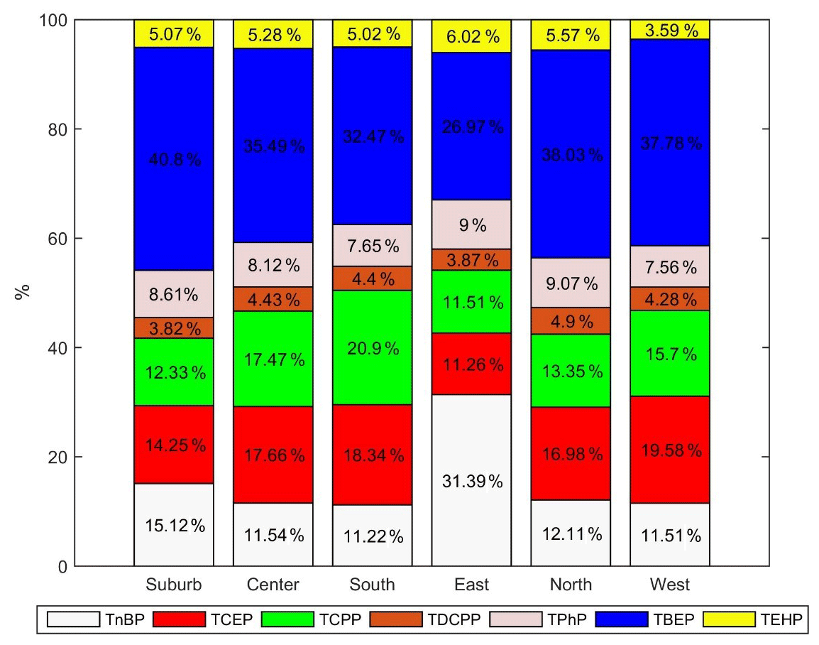
Nonchlorinated OPEs were the predominant OPEs across the city of Chengdu. The annual median concentrations of total OPEs were fairly uniform at the six sites and were influenced mainly by alkylated OPEs. As listed in Table 1, the general trend was that TBEP was the most abundant OPE (annual median concentration: 2.3 ng m−3, 35.3 % of Σ7 OPEs), followed by TCEP (1.1 ng m−3, 16.3 %) ≈ TnBP (1.0 ng m−3, 15.6 %) ≈ TCPP (1.0 ng m−3, 15.0 %) > TPhP (0.5 ng m−3, 8.4 %) > TEHP (0.3 ng m−3, 5.1 %) > TDCPP (0.3 ng m−3, 4.3 %), with the concentrations of TBEP being approximately 7–10 times higher than those of TDCPP and TEHP. The composition profile of OPEs was similar at all sites except for the east site, which had a higher contribution of TnBP. However, TBEP, TCEP, TCPP and TnBP were the dominant OPEs across the city and contributed more than 80 % to Σ7 OPEs. This profile was similar to that in Longyearbyen, Norway, with the primary pollutants being TnBP and TBEP (Möller et al., 2012), as well as the profiles of OPEs in outdoor urban air (TBEP > TCPP > TCEP > TnBP > TPhP) in Stockholm, Sweden (Wong et al., 2018), and Turkey (TBEP > TCPP > TPhP > TEHP > TCEP) (Kurtkarakus et al., 2018). However, these results substantially differed from the report of an urban site in Shanghai that showed TCEP (0.1–10.1 ng m−3, 1.8 ng m−3) > TCPP (0.1–9.7, 1.0 ng m−3) > TPhP (0.06–14.0 ng m−3, 0.5 ng m−3) > TnBP (0.06–2.1 ng m−3, 0.4 ng m−3) > TDCPP (Nd.–23.9 ng m−3, 0.3 ng m−3) and only detected TBEP in 3 out of 116 samples (Nd.–0.7 ng m−3, Nd.) (Ren et al., 2016) and reported data from the Bohai and Yellow seas showing TCPP (43–530 ng m−3; 100 ng m−3, 50 ± 11 %) > TCEP (27–150 ng m−3; 71 ng m−3, 25 ± 7 %) > TiBP (tri-iso-butyl phosphate) (19–210 ng m−3; 57 ng m−3, 14 ± 12 %) > TnBP (3.0–37 ng m−3; 13 ng m−3). Li (2014) determined that the primary pollutant of outdoor air in Nanjing was TCEP, and TBEP was not detected. These differences reflected significant differences in OPE production and usage in different regions, even in the same country. It should be noted that the concentrations of TCPP and TCEP were at the same level in this study, failing to indicate the industrial replacement of TCEP by TCPP in Southwest China; this result differed from the higher concentration of TCPP than TCEP observed due to the industrial replacement of TCEP by TCPP in Europe (Quednow and Püttmann, 2009). This absence of industrial replacement was confirmed by the fact that there are manufacturers and sellers of TCEP and TCPP in Chengdu (https://show.guidechem.com/hainuowei, last access: 28 November 2020, http://www.sinostandards.net/index.php, last access: 28 November 2020), indicating the production of and demand for both TCPP and TCEP in this region.
Table 1The annual median concentrations of OPEs in PM2.5 from Chengdu (ng m−3).
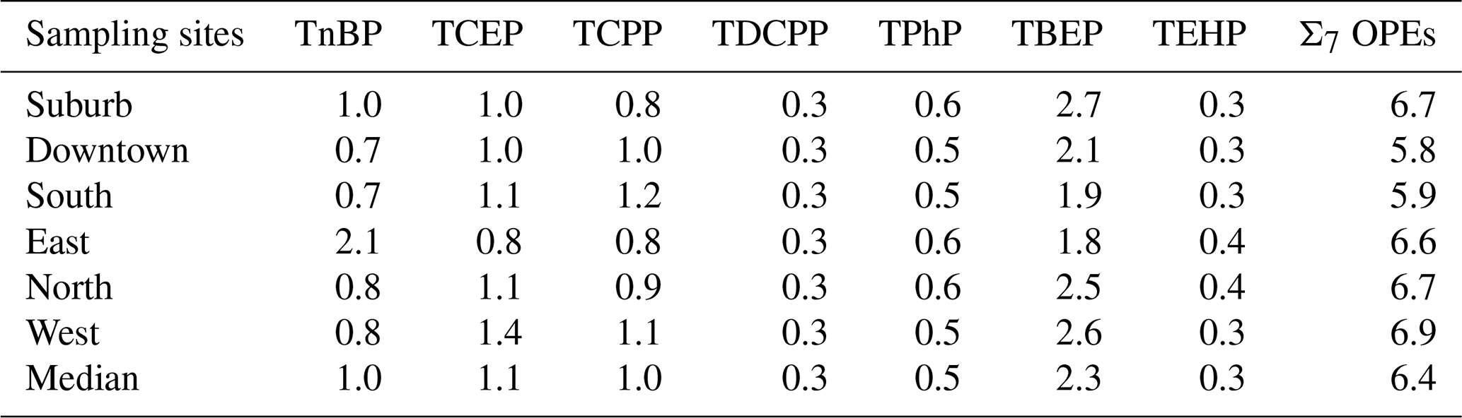
Combined with the data from 2013–2014 (Yin et al., 2015), TBEP was always the dominant OPE during the two sampling periods (2013–2014 and 2014–2015). The Kruskal–Wallis test revealed that TnBP and TCPP had no significant difference between the two sampling periods, but there were significant differences in other kinds of OPEs between the two sampling periods. This result indicated that the production and usage of individual OPEs have changed to a certain degree, suggesting that OPEs should be better investigated and governed with respect to individual compounds.
OPEs can be categorized by whether they are halogenated, alkylated or aryl OPEs. Of the OPEs measured in this study, TCEP, TCPP and TDCPP are halogenated OPEs, TBEP, TnBP and TEHP are alkylated OPEs and TPhP is an aryl OPE. The OPEs in PM2.5 at all sites were dominated by alkylated compounds (55.9 ± 10.1 %), followed by halogenated OPEs (35.8 ± 9.9 %) and aryl OPEs (8.3 ± 4.1 %). Our results are similar to those observed in Bursa, Turkey (Kurtkarakus et al., 2018), where alkylated OPEs accounted for 68 %–95 % of total OPEs, while halogenated OPEs accounted for 3.1 %–29 %, and aryl OPEs accounted for 1.4 %–3.7 %. Wu et al. (2020) also reported that alkyl OPEs dominated the OPE compositional profiles of urban air collected from Chicago and Cleveland. At Longyearbyen, the nonchlorinated OPE concentrations comprised 75 % of the Σ8 OPE concentrations (Salamova et al., 2014a). However, our results are obviously different from those of many studies, with the atmospheric samples collected in urban areas being dominated by chlorinated OPEs (50 %–80 %) (Salamova et al., 2014b; D. Liu et al., 2016; Guo et al., 2016). In our study, nonchlorinated OPEs were dominant in urban and suburban areas across the city.
3.3 Seasonal and spatial variations in OPEs in PM2.5
The mean seasonal concentrations are plotted for the six sampling sites in Fig. 1. The data were quite consistent with our previous study from December 2013 to October 2014 (Yin et al., 2015). The concentrations of OPEs in PM2.5 were fairly uniform throughout the 3 studied years. As shown in Fig. 2, the general order of decreasing average Σ7 OPE concentrations in the suburban area was autumn (8.4 ± 4.3 ng m−3) ≈ winter (8.4 ± 4.5 ng m−3) > spring (7.6 ± 2.2 ng m−3) > summer (3.5 ± 1.1 ng m−3), while in the urban area, the order was autumn (9.30 ± 3.89 ng m−3) > winter (6.63 ± 3.65 ng m−3) > spring (6.36 ± 1.72 ng m−3) > summer (4.60 ± 1.91 ng m−3). The average concentration of Σ7 OPEs in autumn and winter was approximately 2 times that in summer. In summer, turbulent flow accelerated the diffusion of pollutants, leading to the lowest concentration, while higher concentrations of OPEs appeared in autumn and winter because the inversion layer appeared more frequently in autumn and winter, making the diffusion and dilution of pollutants more difficult. This seasonal variation was mostly in line with that at the Shanghai urban site, with an order of autumn (8.4 ng m−3) > winter (7.6 ng m−3) > spring (5.5 ng m−3) > summer (4.4 ng m−3); in that case, the maximum value was also approximately twice the minimum (Ren et al., 2016). In addition, this finding was similar to that in Xinxiang, which showed no significant seasonal changes and only exhibited individual high values in winter. In contrast, Y. Wang et al. (2019) found that the PM2.5-bound fractions of OPEs varied significantly between seasons in Dalian, China, with their concentrations being higher in hot seasons, which may be due to temperature-driven emissions or gas–particle partitioning. Wong et al. (2018) reported that most OPEs in outdoor urban air in Stockholm, Sweden, showed seasonality, with increased concentrations during the warm period. Sühring et al. (2016) reported the temperature dependence of chlorinated OPEs and 2-ethylhexyl diphenyl phosphate (EHDPP) in Arctic air. Wu et al. (2020) reported that median concentrations of Σ OPEs for summer samples were up to 5 times greater than those for winter samples. Similar seasonal patterns were reported by Salamova et al. (2014a) for atmospheric particle-phase OPE concentrations in samples collected from the Great Lakes in 2012. A reasonable explanation is that OPEs are not chemically bound to the materials in which they are used, and higher temperatures may facilitate their emission from buildings and vehicles. However, Shoeib et al. (2014) did not observe any temperature dependence for OPEs in urban air in Toronto, Canada. Thus, previous reports of the temperature dependence of OPEs are not consistent. In our study, correlation analysis between temperature, wind speed, wind direction and Σ7 OPE concentrations was performed. The results showed statistically significant negative correlations between temperature and Σ7 OPEs (R = −0.355, p < 0.01). The lowest concentrations of Σ7 OPEs and individual compounds were observed in summer, suggesting that the OPE level was not dominated by temperature-driven emissions. Gas–particle partitioning and local emission sources may contribute to this variation.
The most obvious difference between these results and those for coastal cities was that the concentrations of almost all OPE monomers in this study were highest in autumn and winter and lowest in summer, suggesting sustained and stable high local emissions in the inland city studied, which is particularly noteworthy. No point sources were identified in summer, and the OPE levels were diluted and diffused in summer due to the higher wind speed than that in winter in the inland city studied. This behavior was different from that of coastal cities: D. Liu et al. (2016) observed the highest TCPP and TCEP concentrations in the summer in Guangzhou, and Javier and Richard (2018) found that the OPEs in spring generally exhibited the lowest concentrations in Bizerte, Tunisia, probably linked to the influence of local meteorological conditions and, to a lesser extent, air mass trajectories.
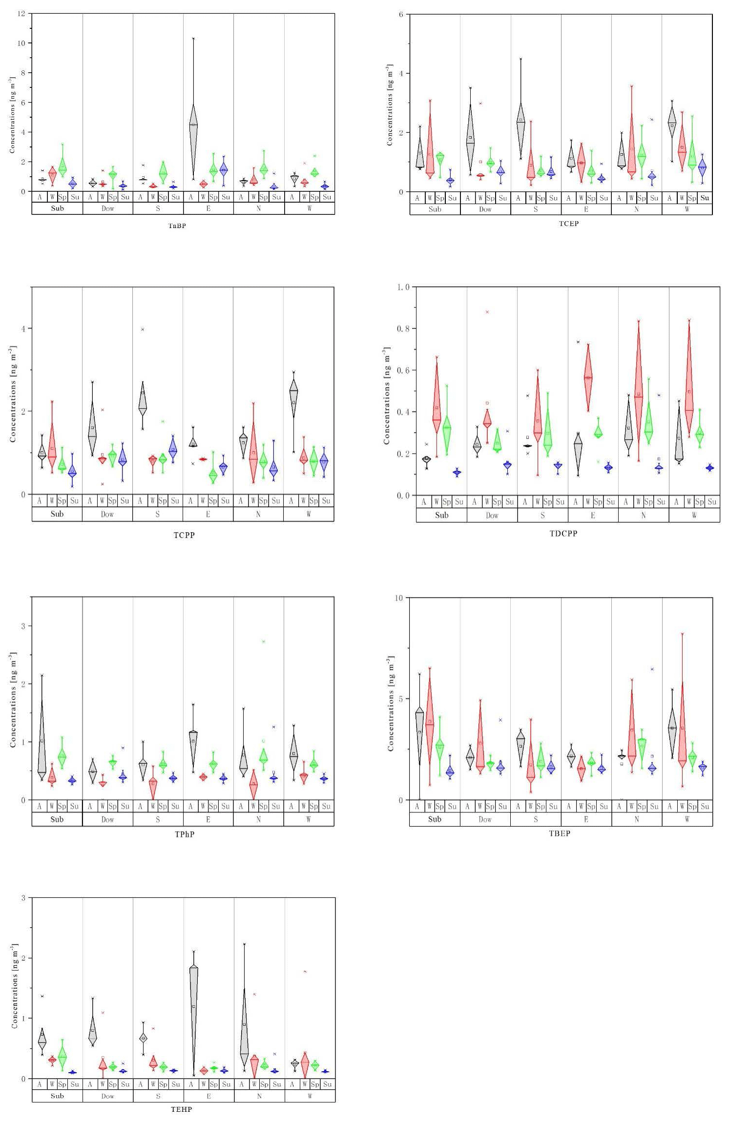
Figure 3The seasonal variation of individual OPEs in PM2.5 from the city of Chengdu. A: autumn, W: winter, Sp: spring, Su: summer, Sub: suburbs, Dow: downtown, S: south, E: east, N: north, W: west.
Although the Kruskal–Wallis test showed no significant variation in Σ7 OPE concentrations across the city, spatial differences were identified in this study. For example, TnBP and TCPP had significant differences among the six sites. In addition, higher concentrations and more dispersed patterns of most OPEs were observed in autumn and winter than in summer (Fig. 3). The concentrations of TEHP in autumn at the eastern and northern sampling sites were more dispersed than those at other sites. The same dispersion pattern was observed for TBEP in winter at the western sampling site, TPhP in autumn at the suburban sampling site and TnBP in autumn at the eastern sampling site, suggesting that extra emission sources existed in autumn or winter. Considering the layout of Chengdu, which spreads out from the central area along the loop line (the first ring road, the second ring road and the third ring road), the uniform patterns of OPE levels and distribution across the city are understandable. Different types of industrial parks in different directions in Chengdu may be the reason for the spatial differences in OPEs. For example, in eastern Chengdu, there are automobile industrial parks and other large industrial parks, while logistics and shoemaking industrial parks are located in the suburbs. The occurrence of unexpectedly high levels of individual OPEs at different sites in autumn might indicate noteworthy emissions. The spatial and seasonal variations in individual OPEs suggest that OPE control and management measures should be taken. Interestingly, in this study, alkyl OPEs dominated at both urban and suburban sites. This finding was extremely different from the results reported by Wu et al. (2020), in which alkyl OPEs dominated at urban sites, chlorinated OPEs were prevalent at rural sites and aryl OPEs were most abundant at remote locations.
Many studies have focused on halogenated OPEs due to their persistence, bioaccumulation and potential human health effects, and they dominate the OPE profile in the air of many cities and other areas (Li et al., 2017). D. Liu et al. (2016) reported that the sum of the concentrations of three halogenated OPEs at 10 urban sites ranged from 0.05 to 12 ng m−3, suggesting that the highest production volume and widest application of OPEs have led to large emissions of OPEs in China in recent years. However, in our study, the mean concentrations of halogenated, alkylated and aryl OPEs were 2.4 ± 1.4, 3.7 ± 2.1 and 0.5 ± 0.4 ng m−3, respectively, which showed that alkylated OPEs dominated the profile of OPEs in PM2.5 in Chengdu. The most notable seasonal variation was observed for alkyl phosphates, followed by halogenated OPEs and aryl OPEs. These results were significantly different from those in other studies that reported that halogenated OPEs had the maximum seasonal variability (Guo et al., 2016; Shoeib et al., 2014).
3.4 Correlation analysis of OPEs
3.4.1 Linkage to environmental factors
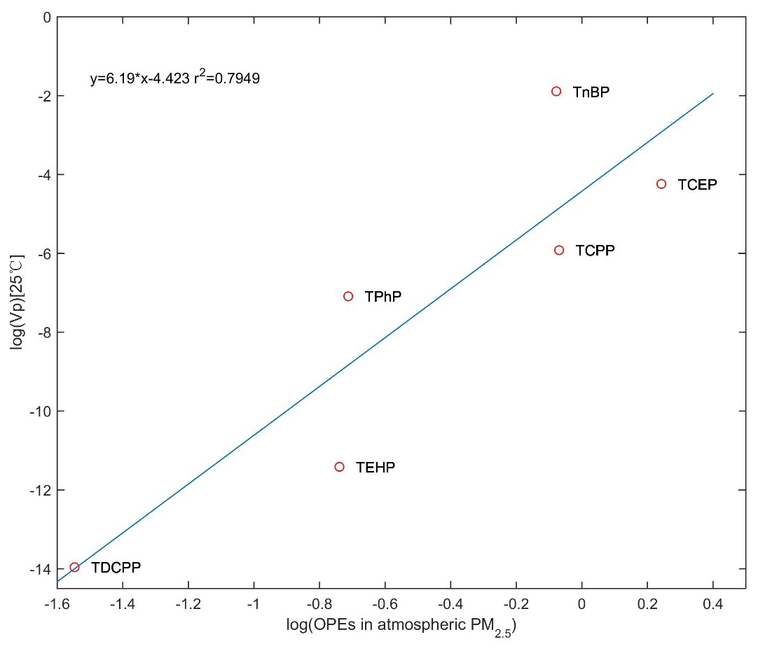
Most OPE monomer concentrations in PM2.5 have a strong linear correlation (R2 = 0.79) with vapor pressure (Fig. 4), suggesting that vapor pressure is an important factor controlling the levels of OPEs in PM2.5, except for TBEP. Generally, the greater the vapor pressure of an OPE is, the more easily the compound can be released into the environment. Therefore, the main sources of most OPEs in Chengdu atmospheric PM2.5 are production processes including OPEs and the phase transition process before they enter into the atmosphere. The boiling points of OPEs are relatively high, so they tend to be adsorbed onto PM2.5 after being released into the environment (Y. Wang et al., 2019), and their gas–particle distributions determine their concentrations in PM2.5. Interestingly, the vapor pressure of TBEP is lower than that of other OPEs, but its concentration in PM2.5 was higher, which indicated that sustained and stable high emission sources, possibly including traffic emission, kept its concentration at a high level (Chen et al., 2020). Sühring et al. (2016) reported that nonhalogenated OPE concentrations in Canadian Arctic air appeared to have diffuse sources or local sources close to the land-based sampling stations.
3.4.2 Correlation between target analytes
Spearman's rank correlation coefficients were used to investigate the potential emission sources for OPEs according to the relationship between individual OPEs in PM2.5 (Fig. 5, Table 2). Figure 5 shows no statistically significant positive correlations between OPE monomers (r < 0.50, p < 0.01). However, Σ7 OPE concentrations were closely related to TBEP, TCEP and TnBP (r = 0.53–0.61, p < 0.01), which further indicated that OPE levels were influenced mainly by the dominant OPE compounds. Comparatively, weak correlations between most OPEs were observed in urban regions (Wang et al., 2018) and Turkey (Kurtkarakus et al., 2018). However, strong correlations between individual OPEs were found in Guangzhou and Taiyuan (Chen et al., 2020).

Figure 5Spearman's rank correlation coefficients between the concentrations of individual OPEs in PM2.5 samples.
Table 2The correlation analysis of individual OPEs in downtown and suburb sampling sites.
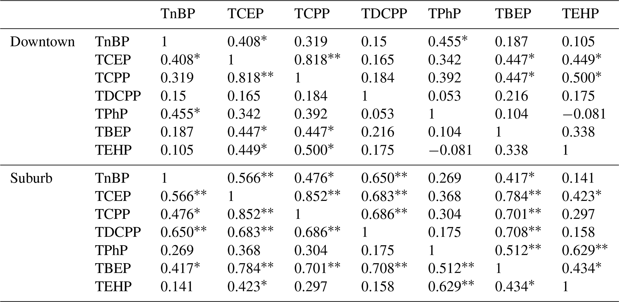
∗ Correlation is significant at the 0.05 level (two-tailed). Correlation is significant at the 0.01 level (two-tailed).
Further analysis results are shown in Table 2. Significant correlations between only TCPP and TCEP at both downtown (r = 0.82, p < 0.01) and suburban sites (r = 0.85, p < 0.01) were observed, indicating the high homology between these two compounds. The inland city in China studied still uses a large number of products containing chlorinated flame retardants, which was confirmed by our previous study of house dust (Liu et al., 2017; Yin et al., 2019). At the downtown site, another significant correlation existed between TEHP and TCEP (r = 0.50, p < 0.01), while other compounds had weak to moderate correlations (r < 0.46, p < 0.01). The downtown area is mainly focused on light industry and software development, and TCPP, TCEP, TnBP, TBEP and TPhP are used in textiles, leather, electronic products and other fields. However, the correlations of each OPE monomer at site A (suburb) were stronger than those in the urban area. The correlations between TnBP and TCEP, TnBP and TDCPP, TCEP and TCPP, TCEP and TDCPP, TCEP and TBEP, TCPP and TDCPP and TCPP and TBEP were all extremely significant. This result indicated that the pollution in the suburbs was commixed and influenced by many kinds of pollution sources.
3.4.3 Correlation analysis of OPEs and PM2.5 concentrations
SPSS software was used to produce scatter plots to analyze the relationship between the concentrations of OPE monomers and PM2.5. As displayed in Fig. S2, only weak to moderate correlations were observed between most OPEs and PM2.5, except for a significant correlation between TDCPP and PM2.5 (r = 0.53, p < 0.01), which suggests that continuous and relatively constant local emissions were the main sources. This result was similar to that reported for Taiyuan (Guo et al., 2016), where no correlation was found between the concentrations of OPEs and the concentration of particulate matter. However, this result differed from that in Xinxiang (Shen et al., 2016), where the concentrations of OPEs and PM2.5 had a significant correlation (r = 0.85c), and high values of OPEs ∕ PM2.5 were related to the contribution of air masses from heavily polluted areas (Henan and Jiangsu provinces), while low OPEs–PM2.5 values were due to air masses from Shanxi–Gansu and Neimenggu provinces. Chen et al. (2020) found that there was a significant correlation (p < 0.05) between the concentrations of Σ11 OPEs and PM2.5 at some sampling sites but not at a site located in the urban region in Guangzhou with potential additional pollution sources.
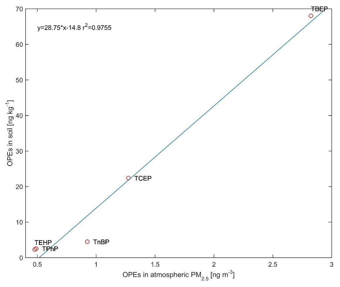
3.4.4 Correlation analysis of OPEs in PM2.5 and soil
Due to the low detection frequency of TCPP and TDCPP in the soil (Yin et al., 2016), the relationships of the other five OPE monomers in the soil and in atmospheric PM2.5 are presented in Fig. 6. A very strong linear relationship was obtained between the OPEs in soil and in PM2.5 (R2 = 0.98, p < 0.01), indicating that atmospheric PM2.5 settling is an important source of OPEs in the soil, just as soil is a source for OPEs in the air.
3.4.5 Correlation analysis of OPEs in indoor and outdoor air
The OPE profile in outdoor air in this study was TBEP > TCEP > TnBP > TCPP > TPhP > TEHP > TDCPP, which was different from that of indoor dust reported in our previous study (Liu et al., 2017): TPhP > TCPP > TnBP > TDCPP > TBEP > TCEP > TEHP. TPhP is used as an important alternative to decabrominated diphenyl ether (deca-BDE), which is typically used as a flame retardant in electrical and electronic products. In addition, plastic films and rubber may be important sources of TPhP. Thus, OPEs in indoor dust mainly come from the indoor environment and are related to human activities, not from outdoor air. In addition to the different usages of OPEs, many factors may also lead to differences between indoor and outdoor OPEs. For example, TBEP has the shortest atmospheric half-life, which may explain why its dominance in indoor samples was not observed for its outdoor counterparts. Studies in Sweden (Wong et al., 2018) reported that the concentrations of OPEs in indoor air followed the order TCPP > TCEP > TBEP > TnBP > TPhP, and those in outdoor urban air followed the order TBEP > TCPP > TCEP > TnBP > TPhP (Wong et al., 2018), which also indicated differences in OPE profiles in indoor and outdoor air. They found that activities in buildings, e.g., floor cleaning, polishing, construction, introduction of new electronics and changes in ventilation rate, could be key factors controlling the concentration of indoor air pollutants, while the observed seasonality for OPEs in outdoor air was due to changes in primary emissions.
3.5 Source apportionment of OPEs
3.5.1 Backward trajectory model analysis
Backward trajectory cluster analysis (HYSPLIT4), which combines the horizontal and vertical motion of the atmosphere and can analyze the transport, migration and diffusion of atmospheric pollutants, was used in this study. The height of 500 m above ground level (a.g.l.) can best represent the characteristics of the wind field associated with this process, and HYSPLIT4 was used to obtain the 500 m a.g.l. 24 h backward trajectory during the sampling period in Chengdu. During the sampling period, the air masses were mainly from the northeastern and southern parts of Sichuan Province, including Mianyang, Deyang, Renshou and Chengdu, and a few of the trajectories came from Chongqing and other places in Gansu Province. Therefore, during the sampling period, Chengdu was mainly affected by air masses from eastern Sichuan.
In different seasons, the air sources always came from the southern or northern regions of Chengdu. In spring, Chengdu was influenced by air masses from the southern region, which could be divided into three paths: (a) from Ya'an through Renshou to Chengdu, (b) from Leshan and Yibin and (c) from Chongqing through Ziyang to Chengdu. The concentrations of OPEs at the northern and suburban sites were relatively high in spring. During the summer period, Chengdu was mainly influenced by air masses from both the southern areas (Yibin, Zigong and others) and the northern areas (Gansu Province, Guangyuan and Mianyang), but there was no significant difference in OPE concentrations at each sampling site, nor in autumn and winter. Combined with the results of backward trajectory cluster analysis and the concentrations of OPEs at each sampling site, the concentrations of OPEs had no obvious change. This result suggested that OPEs were not affected by exogenous pollution but were mainly affected by local sources in Chengdu. These results are consistent with the meteorological and topographic conditions. Chengdu's wind has always been breezy with a much lower strength than that of coastal cities or other inland cities (https://baike.baidu.com/item/%E6%88%90%E9%83%BD/128473?fr=aladdin). The wind direction is relatively constant, mainly from the north or north–northeast. In addition, Chengdu is a city located in the interior of China, surrounded by the Qinghai–Tibet Plateau, the Qinling Mountains, etc. These topographic and meteorological conditions block the influence of foreign sources on Chengdu's atmosphere, which further explains why the pollution of OPEs in PM2.5 was controlled by endogenous pollution, not by exogenous pollution.
3.5.2 Principal component analysis
Principal component analysis (PCA) of OPEs was carried out using SPSS. The normalized correlation coefficient matrix of the original data for each sampling site showed that there was a strong correlation between TCPP and TCEP, TCEP and TBEP and TnBP and TPhP, which satisfied the condition of dimensionality reduction of PCA. Two principal component factors were obtained in this study. The cumulative contribution of the two principal component factors was 62.3 %, which can basically explain the data. The results are shown in Table S1. For factor 1, there was a large load on TCEP, TCPP and TBEP and a moderate load on TDCPP. Factor 1 can represent sources of OPEs from the plastic industry, interior decoration and traffic emissions, with a contribution ratio of 34.5 % (Marklund et al., 2005; Regnery et al., 2011). Factor 2 has a higher load on TnBP, TEHP and TPhP. The highest load was on TnBP, which is often used as a high-carbon alcohol defoamer, mostly in industries that do not come into contact with food and cosmetics, as well as in antistatic agents and extractants of rare earth elements. TEHP can be used as an antifoaming agent, hydraulic fluid and so on. TPhP is typically used in electrical and electronic products, plastic films and rubber (Stevens et al., 2006; Wei et al., 2015). Factor 2 can be attributed to the chemical, mechanical and electrical industries, and its contribution ratio was 27.8 %.
3.5.3 PMF model analysis
The basic principle of the positive matrix factorization (PMF) method is to decompose a sample matrix into a factor contribution matrix and factor component spectrum. The source type of the factor is judged according to the factor component spectrum, and then the contribution ratio of the source is determined. The PMF5.0 model developed by US EPA was used. The uncertainty value was input according to the guideline of PMF. The following methods were used to determine the optimal scheme of the three factors: (1) measurement of the Q values and (2) comparison of the predicted concentration with the original measured concentration to evaluate the accuracy of the model fit. From the 149 samples collected in Chengdu, 132 valid samples were selected to participate in the model calculation, and three factors were obtained. From the 149 samples collected in Chengdu, 132 valid samples were selected to participate in the model calculation, and three factors were determined. TPhP was the only chemical with a residual (4.0) greater than 3. The concentrations of OPEs satisfied the normal distribution. The components of factor 1 were complex. Factor 1 contributed 71.0 %, 70.7 % and 70.9 % to TCEP, TCPP and TEHP, respectively, and 58.3 % to TPhP. Factor 1 was deduced to be the plastics and electrical industry and indoor source emissions (Stevens et al., 2006). Factor 2 contributed the most to TBEP (78.0 %), followed by TDCPP (44.7 %), while it did not contribute to TnBP. Therefore, factor 2 was deduced to be the food and cosmetics industry and traffic emissions (Marklund et al., 2005). Factor 3 contributed 71.7 % of the total TnBP and was deduced to be a chemical industrial source (Regnery et al., 2011).
Compared to the levels of OPEs in other cities, the levels of OPEs measured in this study were comparable to or even higher than those in most other studies. This result suggests that during the shift of labor-intensive manufacturing from coastal developed areas to inland regions, OPEs were widely used in industrial and manufacturing processes in Southwest China, which should arouse concern.
This intensive sampling campaign of urban and suburban areas found no significant spatial variability in Σ7 OPEs across Chengdu, China, but the most notable seasonal variation was observed for alkyl phosphate, followed by halogenated OPEs and aryl OPEs. Higher concentrations and more dispersed patterns of OPEs were observed in autumn and winter than in summer, with TBEP, TCEP, TCPP and TnBP being the dominant compounds. The occurrence of unexpectedly high levels of individual OPEs at different sites in autumn might indicate that there were noteworthy emissions. PCA showed that the main sources of OPEs in PM2.5 include plastic industry, interior decoration and traffic emission (34.5 %) and the chemical, mechanical and electrical industries (27.8 %). PMF showed that the main sources were the plastics and electrical industry and indoor source emissions. OPEs have a wide range of physical and chemical properties, and combined with the differences in their behavior identified in this study, the management of OPEs as individual compounds instead of a single chemical class should be considered. In addition, due to the special topography and meteorological conditions of the inland city studied, the distribution and seasonal variation of OPEs in the air in this study were significantly different from those of most coastal cities and ocean locations. The sustained and stable high local emissions are particularly noteworthy. Chlorinated phosphates, especially TCPP and TCEP, which are highly toxic and persistent in the environment, had high concentrations in this study. Their usage and source emissions should be controlled.
The experimental data are available at https://doi.org/10.6084/m9.figshare.13312553.v1 (Yin, 2020).
The supplement related to this article is available online at: https://doi.org/10.5194/acp-20-14933-2020-supplement.
HY designed the experiments and created the methodology with SL. JL and SL carried the experiments out as the team leader. JL, SL, YL, and XD sampled and collected the experimental data. SL arranged and visualized the data. JL and DW wrote the original draft. SL revised the charts. HY carried out the review and editing of the paper with contributions from all co-authors.
The authors declare that they have no conflict of interest.
We gratefully acknowledge support from the National Natural Science Fund. We are grateful to Zengwu Wang for providing Fig. S1. We thank Hui Zhang and Shuhong Fang for helpful comments and contributions to the editing of the paper.
This research has been supported by the National Natural Science Foundation of China (grant nos. 41773072, 21407014, 41831285).
This paper was edited by Jason Surratt and reviewed by two anonymous referees.
Blum, A., Behl, M., Birnbaum, L. S., Diamond, M. L., Phillips, A., Singla, V., Sipes, N. S., Stapleton, H. M., and Venier, M.: Organophosphate ester flame retardants: are they a regrettable substitution for polybrominated diphenyl ethers?, Environ. Sci. Technol. Lett., 6, 638–649, https://doi.org/10.1021/acs.estlett.9b00582, 2019.
Celano, R., Rodríguez, I., Cela, R., Rastrelli, L., and Piccinelli, A. L.: Liquid chromatography quadrupole time-of-flight mass spectrometry quantification and screening of organophosphate compounds in sludge, Talanta, 118, 312–320, https://doi.org/10.1016/j.talanta.2013.10.024, 2014.
Chen, Y. Y., Song, Y. Y., Chen, Y. J., Zhang, Y. H., Li, R. J., Wang, Y. J., Qi, Z. H., Chen, F. H., and Cai, Z. W.: Contamination profiles and potential health risks of organophosphate flame retardants in PM2.5 from Guangzhou and Taiyuan, China, Environ. Int., 134, 105343, https://doi.org/10.1016/j.envint.2019.105343, 2020.
Clark, A. E., Yoon, S., Sheesley, R.J., and Usenko, S.: Spatial and temporal distributions of organophosphate ester concentrations from atmospheric particulate matter samples collected across Houston, TX, Environ. Sci. Technol., 51, 4239–4247, https://doi.org/10.1021/acs.est.7b00115, 2017.
Cristale, J. and Lacorte, S.: Development and validation of a multiresidue method for the analysis of polybrominated diphenyl ethers, new brominated and organophosphorus flame retardants in sediment, sludge and dust, J. Chromatogr. A., 1305, 267–275, https://doi.org/10.1016/j.chroma.2013.07.028, 2013.
Cristale, A., García Vázquez, A., Barata, C., and Lacorte, S.: Priority and emerging flame retardants in rivers: occurrence inwater and sediment, Daphniamagna toxicity and risk assessment, Environ. Int., 59, 232–243, https://doi.org/10.1016/j.envint.2013.06.011, 2013.
Du, Z., Wang, G., Gao, S., and Wang, Z.: Aryl organophosphate flame retardants induced cardiotoxicity during zebrafish embryogenesis: by disturbing expression of the transcriptional regulators, Aquat. Toxicol., 161, 25–32, https://doi.org/10.1016/j.aquatox.2015.01.027, 2015.
Exponent: California bans flame retardants in certain consumer products, available at: https://www.exponent.com/knowledge/alerts/2018/09/california-bans-flame-retardants/?pageSize=NaN&pageNum=0&loadAllByPageSize=true (last access: 15 February 2020), 2018.
Guo, Z. M., Liu, D., Shen, K. J., Li, J., Yu, Z. Q., and Zhang, G.: Concentration and seasonal variation of organophosphorus flame retardants in PM2.5 of Taiyuan City, China, Earth and environment, 44, 600–604, https://doi.org/10.14050/j.cnki.1672-9250.2016.06.002, 2016 (in Chinese).
Javier, C. J. and Richard, S.: Atmospheric particle-bound organophosphate ester flame retardants and plasticizers in a North African Mediterranean coastal city (Bizerte, Tunisia), Sci. Total Environ., 642, 383–393, https://doi.org/10.1016/j.scitotenv.2018.06.010, 2018.
Kanazawa, A., Saito, I., Araki, A., Takeda, M., Ma, M., Saijo, Y., and Kishi, R.: Association between indoor exposure to semi-volatile organic compounds and building-related symptoms among the occupants of residential dwellings, Indoor. Air., 20, 72–84, https://doi.org/10.1111/j.1600-0668.2009.00629.x, 2010.
Kim, J. W., Isobe, T., Chang, K. H., Amano, A., Maneja, R. H., Zamora, P. B., Siringan, F. P., and Tanabe, S.: Levels and distribution of organophosphorus flame retardants and plasticizers in fishes from Manila Bay, the Philippines, Environ. Pollut., 159, 3653–3659, https://doi.org/10.1016/j.envpol.2011.07.020, 2011.
Kurtkarakus, P., Alegria, H., Birgul, A., Gungormus, E., and Jantunen, L.: Organophosphate ester (OPEs) flame retardants and plasticizers in air and soil from a highly industrialized city in Turkey, Sci. Total. Environ., 625, 555–565, https://doi.org/10.1016/j.scitotenv.2017.12.307, 2018.
Lai, S., Xie, Z., Song, T., Tang, J., Zhang, Y., and Mi, W.: Occurrence and dry deposition of organophosphate esters in atmospheric particles over the Northern South China Sea, Chemosphere, 127, 195–200, https://doi.org/10.1016/j.chemosphere.2015.02.015, 2015.
Li, J.: Occurrence and health risk assessment of organophosphate flame retardants in drinking water and air, Nanjing University, Nanjing, China, 2014.
Li, J., Yu, N., Zhang, B., Jin, L., Li, M., Hu, M., Zhang, X., Wei, S., and Yu, H.: Occurrence of organophosphate flame retardants in drinking water from China, Water. Res., 54, 53–61, https://doi.org/10.1016/j.watres.2014.01.031, 2014.
Li, J., Xie, Z., Mi, W., Lai, S., Tian, C., and Emeis, K. C.: Organophosphate esters in air, snow and seawater in the north Atlantic and the Arctic, Environ. Sci. Technol., 51, 6887–6896, https://doi.org/10.1021/acs.est.7b01289, 2017.
Li, J., Tang, J., Mi, W., Tian, C. G., Emeis, K. C., Ebinghaus, R., and Xie, Z. Y.: Spatial distribution and seasonal variation of organophosphate esters in air above the Bohai and Yellow Seas, China, Environ. Sci. Technol., 52, 89–97, https://doi.org/10.1021/acs.est.7b03807, 2018.
Liu, D., Lin, T., Shen, K. J., Li, J., Yu, Z. Q., and Zhang, G.: Occurrence and concentrations of halogenated flame retardants in the atmospheric fine particles in Chinese cities, Environ. Sci. Technol., 50, 9846–9854, https://doi.org/10.1021/acs.est.6b01685, 2016.
Liu, Q., Yin, H. L., Li, D., Deng, X., Fang, S. H., and Sun, J.: Distribution characteristic of OPEs in indoor dust and its health risk, China. Environ. Sci., 37, 2831–2839, https://doi.org/10.3969/j.issn.1000-6923.2017.08.004, 2017.
Liu, R., Lin, Y., Liu, R., Hu, F., Ruan, T., and Jiang, G.: Evaluation of two passive samplers for the analysis of organophosphate esters in the ambient air, Talanta, 147, 69–75, https://doi.org/10.1016/j.talanta.2015.09.034, 2016.
Marklund, A., Andersson, B., and Haglund, P.: Traffic as a source of organophosphorus flame retardants and plasticizers in snow, Environ. Sci. Technol., 39, 3555–3562, https://doi.org/10.1021/es0482177, 2005.
McDonough, C. A., De Silva, A. O., Sun, C., Cabrerizo, A., Adelman, D., Soltwedel, T., Bauerfeind, E., Muir, D. C. G., and Lohmann, R.: Dissolved organophosphate esters and polybrominated diphenyl ethers in remote marine environments: Arctic surface water distributions and net transport through Fram Strait, Environ. Sci. Technol., 52, 6208–6216, https://doi.org/10.1021/acs.est.8b01127, 2018.
Möller, A., Xie, Z., Caba, A., Sturm, R., and Ebinghaus, R.: Organophosphorus flame retardants and plasticizers in the atmosphere of the North Sea, Environ. Pollut., 159, 3660–3665, https://doi.org/10.1016/j.envpol.2011.07.022, 2011.
Möller, A., Sturm, R., Xie, Z., Cai, M., He, J., and Ebinghaus, R.: Organophosphorus flame retardants and plasticizers in airborne particles over the northern pacific and Indian Ocean toward the polar regions: evidence for global occurrence, Environ. Sci. Technol., 46, 3127–3134, 2012.
Ohura, T., Amagai, T., Senga, Y., and Fusaya, M.: Organic air pollutants inside and outside residences in Shimizu, Japan: levels, sources and risks, Sci. Total. Environ., 366, 485–499, https://doi.org/10.1016/j.scitotenv.2005.10.005, 2006.
Quednow, K. and Püttmann, W.: Temporal concentration changes of DEET, TCEP, terbutryn, and nonylphenols in freshwater streams of Hesse, Germany: possible influence of mandatory regulations and voluntary environmental agreements, Environ. Sci. Pollut. R., 16, 630–640, https://doi.org/10.1007/s11356-009-0169-6, 2009.
Regnery, J., Püttmann, W., Merz, C., and Berthold, G.: Occurrence and distribution of organophosphorus flame retardants and plasticizers in anthropogenically affected groundwater, J. Environ. Monitor., 13, 347–354, https://doi.org/10.1039/C0EM00419G, 2011.
Ren, G., Chen, Z., Feng, J., Ji, W., Zhang, J., and Zheng, K.: Organophosphate esters in total suspended particulates of an urban city in East China, Chemosphere, 164, 75–83, https://doi.org/10.1016/j.chemosphere.2016.08.090, 2016.
Salamova, A., Ma, Y., Venier, M., and Hites, R. A.: High levels of organophosphate flame retardants in the great lakes atmosphere, Environ. Sci. Technol., 46, 8653–8660, https://doi.org/10.1021/ez400034n, 2014a.
Salamova, A., Hermanson, M. H., and Hites, R. A.: Organophosphate and halogenated flame retardants in atmospheric particles from a European Arctic site, Environ. Sci. Technol., 48, 6133–6140, https://doi.org/10.1021/es500911d, 2014b.
Shen, K. J., Zhang, X. Y., Liu, D. Geng, X. F., Sun, J. H., and Li, J.: Characterization and seasonal variation of carbonaceous aerosol in urban atmosphere of a typical city in North China, Ecology. Environ. Sci., 25, 458–463, https://doi.org/10.16258/j.cnki.1674-5906.2016.03.013, 2016 (in Chinese).
Shoeib, M., Ahrens, L., Jantunen, L., and Harner, T.: Concentrations in air of organobromine, organochlorine and organophosphate flame retardants in Toronto, Canada, Atmos. Environ., 99, 140–147, https://doi.org/10.1016/j.atmosenv.2014.09.040, 2014.
State of California: Safer consumer products (SCP) information management system, available at: https://calsafer.dtsc.ca.gov/cms/search/?type=Chemical, last access: 21 February 2020.
Stevens, R., van Es, D. S., Bezemer, R., and Kranenbarg, A.: The structure-activity relationship of fire retardant phosphorus compounds in wood, Polym. Degrad. Stabil., 91, 832–841, https://doi.org/10.1016/j.polymdegradstab.2005.06.014, 2006.
Sühring, R., Diamond, M. L., Scheringer, M., Wong, F., Puko, M., Stern, G., Burt, A., Hung, H., Fellin, P., Li, H., and Jantunen, L. M.: Organophosphate esters in Canadian Arctic air: occurrence, levels and trends, Environ. Sci. Technol., 50, 7409–7415, https://doi.org/10.1021/acs.est.6b00365, 2016.
Van der Veen, I. and de Boer, J.: Phosphorus flame retardants: properties, production, environmental occurrence, toxicity and analysis, Chemosphere, 88, 1119–1153, https://doi.org/10.1016/j.chemosphere.2012.03.067, 2012.
Wang, D., Wang, P., Wang, Y. W., Zhang, W. W., Zhu, C. F., Sun, H. Z., Matsiko, J., Zhua, Y., Li, Y. M., Meng, W. Y., Zhang, Q. H., and Jiang, G. B.: Temporal variations of PM2.5-bound organophosphate flame retardant in different microenvironments in Beijing, China, and implications for human exposure, Sci. Total Environ., 666, 226–234, https://doi.org/10.1016/j.scitotenv.2019.02.076, 2019.
Wang, T., Ding. N., Wang. T., Chen. S. J., Luo. X. J., and Mai. B. X.: Organophosphorus esters (OPEs) in PM2.5 in urban and e-waste recycling regions in southern China: concentrations, sources, and emissions, Environ. Res., 167, 437–444, https://doi.org/10.1016/j.envres.2018.08.015, 2018.
Wang, X., He, Y., Li, L., Feng, Z., and Luan, T.: Application of fully automatic hollow fiber liquid phase microextraction to assess the distribution of organophosphate esters in the Pearl River estuaries, Sci. Total. Environ., 470/471, 263–269, https://doi.org/10.1016/j.scitotenv.2013.09.069, 2013.
Wang, Y., Bao, M. J., Tan, F., Qu, Z. P., Zhang, Y. W., and Chen, J. W.: Distribution of organophosphate esters between the gas phase and PM2.5 in urban Dalian, China, Environ. Pollut., 259, 113882, https://doi.org/10.1016/j.envpol.2019.113882, 2019.
Wei, G. L., Li, D. Q., Zhuo, M. N., Liao, Y. S., Xie, Z. Y., Guo, T. L., Li, J. J., Zhang, S. Y., and Liang, Z. Q.: Organophosphorus flame retardants and plasticizers: sources, occurrence, toxicity and human exposure, Environ. Pollut., 196, 29–46, https://doi.org/10.1016/j.envpol.2014.09.012, 2015.
WHO (World Health Organization): Flame retardants: tris (Chloropropyl) phosphate and tris (2-chlorethyl) phosphate, Environmental Health Criteria, 209, 23–46, https://doi.org/10.1002/9780470986738.refs, 1998.
Wong, F., Wit, C. A. D., and Newton, S. R.: Concentrations and variability of organophosphate esters, halogenated flame retardants, and polybrominated diphenyl ethers in indoor and outdoor air in Stockholm, Sweden, Environ. Pollut., 240, 514–522, https://doi.org/10.1016/j.envpol.2018.04.086, 2018.
Wu, Y., Venier, M., and Salamova, A.: Spatioseasonal variations and partitioning behavior of organophosphate esters in the Great Lakes atmosphere, Environ. Sci. Technol., 54, 5400–5408, https://doi.org/10.1021/acs.est.9b07755, 2020.
Yin, H. L.: Data for seasonality, distribution and sources of organophosphate esters in PM2.5 from an inland urban city in Southwest China, figshare, https://doi.org/10.6084/m9.figshare.13312553.v1, 2020.
Yin, H. L., Li, S. P., Ye, Z. X., Yang, Y. C., Liang, J. F., and You, J. J.: Pollution level and sources of organic phosphorus esters in airborne PM2.5 in Chengdu City, Environ. Sci., 36, 3566–3572, https://doi.org/10.13227/j.hjkx.2015.10.003, 2015 (in Chinese).
Yin, H. L., Li, S. P., Ye, Z. X., Liang, J. F., and You, J. J.: Pollution characteristics and sources of OPEs in the soil of Chengdu City, Ac. Scientiae. Circumstantiae, 36, 606–613, https://doi.org/10.13671/j.hjkxxb.2015.0489, 2016.
Yin, H. L., Wu, D., You, J. J., Li, S. P., Deng, X., Luo, Y., and Zheng, W. Q.: Occurrence, distribution, and exposure risk of organophosphate esters in street dust from Chengdu, China, Arch. Environ. Con. Tox., 76, 617–629, https://doi.org/10.1007/s00244-019-00602-3, 2019.