the Creative Commons Attribution 4.0 License.
the Creative Commons Attribution 4.0 License.
 | 02 Dec 2020
Effects of 3D electric field on saltation during dust storms: an observational and numerical study
Huan Zhang
You-He Zhou
Particle triboelectric charging, being ubiquitous in nature and industry, potentially plays a key role in dust events, including the lifting and transport of sand and dust particles. However, the properties of the electric field (E field) and its influences on saltation during dust storms remain obscure as the high complexity of dust storms and the existing numerical studies are mainly limited to the 1D E field. Here, we quantify the effects of the real 3D E field on saltation during dust storms through a combination of field observations and numerical modelling. The 3D E fields in the sub-metre layer from 0.05 to 0.7 m above the ground during a dust storm are measured at the Qingtu Lake Observation Array site. The time-varying means of the E field series over a certain timescale are extracted by the discrete wavelet transform and ensemble empirical mode decomposition methods. The measured results show that each component of the 3D E field data roughly collapses on a single third-order polynomial curve when normalized. Such 3D E field data within a few centimetres of the ground have never been reported and formulated before. Using the discrete element method, we then develop a comprehensive saltation model in which the triboelectric charging between particle–particle midair collisions is explicitly accounted for, allowing us to evaluate the triboelectric charging in saltation during dust storms properly. By combining the results of measurements and modelling, we find that, although the vertical component of the E field (i.e. 1D E field) inhibits sand transport, the 3D E field enhances sand transport substantially. Furthermore, the model predicts that the 3D E field enhances the total mass flux and saltation height by up to 20 % and 15 %, respectively. This suggests that a 3D E field consideration is necessary if one is to explain precisely how the E field affects saltation during dust storms. These results further improve our understanding of particle triboelectric charging in saltation and help to provide more accurate characterizations of sand and dust transport during dust storms.
- Article
(7159 KB) - Full-text XML
-
Supplement
(1623 KB) - BibTeX
- EndNote


Contact or triboelectric charging is ubiquitous in dust events (Schmidt et al., 1998; Zheng et al., 2003; Kok and Renno, 2008; Lacks and Sankaran, 2011; Harrison et al., 2016). The pioneering electric field (E field) measurements in dust storms by Rudge (1913) showed that the vertical atmospheric E field was substantially increased to 5–10 kV m−1, and its direction reversed (became upward-pointing) during a severe dust storm. Later measurements in dust storms found a downward-pointing (Esposito et al., 2016), upward-pointing (Bo and Zheng, 2013; Yair et al., 2016; Zhang and Zheng, 2018), and even alternating vertical E field, which continually reverses direction (Kamra, 1972; Williams et al., 2009), with a magnitude of up to ∼100 kV m−1.
The significant influences of the E field on pure saltation (that is, in the absence of suspended dust and aerosol particles) have been verified, both numerically (e.g. Kok and Renno, 2008; Zhang et al., 2014) and experimentally (e.g. Rasmussen et al., 2009; Esposito et al., 2016). The effects of the E field on saltation during dust storms, however, remain obscure. A clear difference between the numerical simulation and field measurement is that the numerical simulation of pure saltation showed a reduction in the saltation mass flux by the E field (e.g. Zheng et al., 2003; Kok and Renno, 2008), whereas recent field measurements found a dramatic increase in the dust concentration during dust storms (up to a factor of 10) by the E field (Esposito et al., 2016), suggesting that the E field might enhance the saltation mass flux during dust storms. This is probably because only the vertical component of the E field (i.e. 1D) should be considered in pure saltation, but there also, in fact, exist streamwise and spanwise components of E field in dust events. For example, Jackson and Farrell (2006) recorded the horizontal component of the E field of up to 120 kV m−1 in dust devils. Zhang and Zheng (2018) also found the streamwise and spanwise components (termed the horizontal component) of the E field of up to 150 kV m−1 in dust storms. Hence, the E field is actually 3D during dust storms. In many cases, the magnitude of the horizontal component is larger than that of the vertical component (Bo and Zheng, 2013; Zhang and Zheng, 2018). The horizontal component should therefore not be neglected when evaluating the role of the E field in saltation during dust storms.
Most field observations, such as Schmidt et al. (1998) and Bo et al. (2014), have studied the electrical properties of sand particles in dust events. However, many environmental (lurking) factors, such as relative humidity, soil moisture, surface crust, etc., cannot be fully controllable (recorded) in these field observations. The uncertainties in the field observations provide the motivation for numerical studies of the particle triboelectric charging in saltation. In addition, unlike pure saltation, the dust storm is a very complex dusty phenomenon that is made up of numerous polydisperse particles embedded in a high Reynolds number turbulent flow. Such a high complexity of dust storms challenges the accurate simulation of the 3D E field in dust storms. It is therefore more straightforward to characterize the 3D E field experimentally.
In this study, we evaluate the effects of the 3D E field on saltation during dust storms by combining measurements and modelling. To reveal the properties of the 3D E field, we simultaneously measured the 3D E fields in the sub-metre layer from 0.05 to 0.7 m above the ground during a dust storm. Such a vertical profile of the 3D E field in the sub-metre layer has not been previously characterized. To reveal how the 3D E field affects saltation during dust storms, we develop a comprehensive numerical model of particle triboelectric charging in saltation. In this model, the charge transfers between contacting particles are explicitly calculated, but the 3D E field is formulated directly, based on the data measured in our measurements, due to its huge challenges in modelling. The effects of various important parameters, such as the density of charged species and the height-averaged time-varying mean of the 3D E field, are also investigated and described herein.
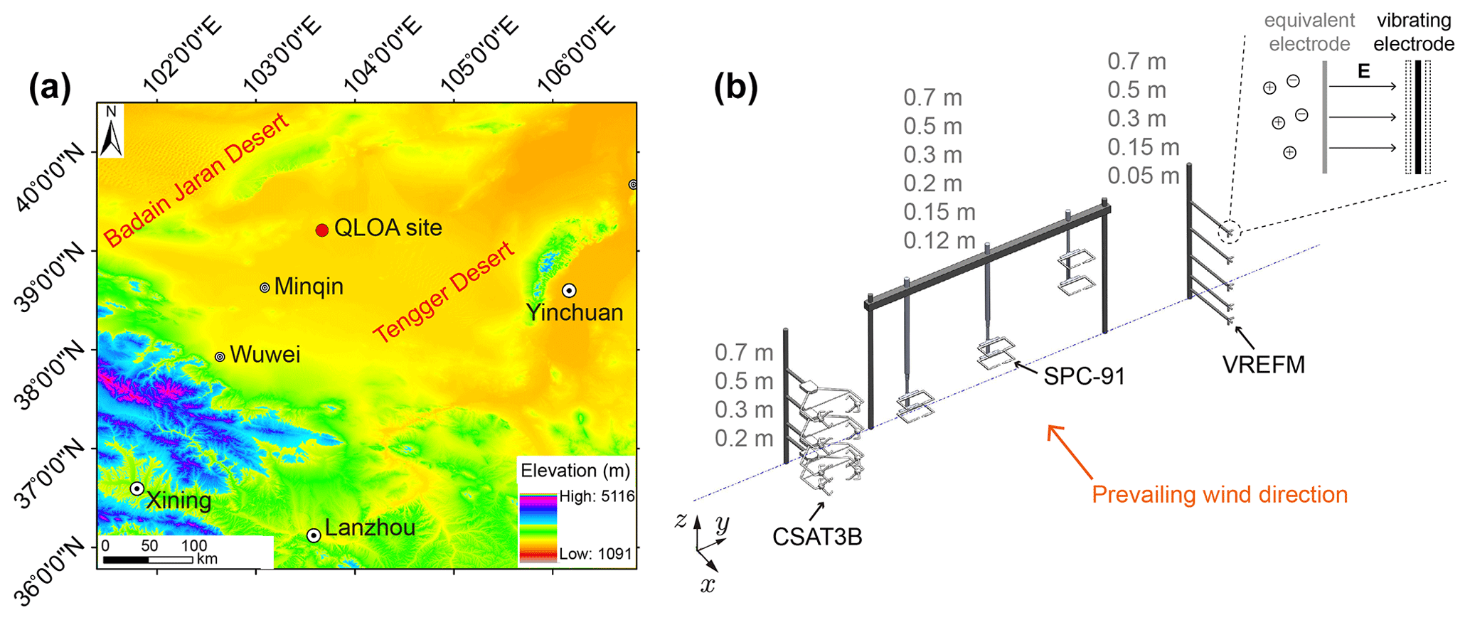
Figure 1Map of the Qingtu Lake Observation Array (QLOA) site and the layout of all instruments. (a) The QLOA site is located between the Badain Jaran Desert and the Tengger Desert, approximately 90 km northeast of Minqin, Gansu, China. (b) Four CSAT3B sensors were mounted at a 0.2–0.7 m height, respectively; six sand particle counter (SPC)-91 sensors were mounted at a 0.12–0.7 m height, respectively; a total of 15 vibrating-reed E field mill (VREFM) sensors were mounted to measure the 3D E field at a 0.05–0.7 m height, respectively (that is, at each measurement point, three VREFM sensors are mutually perpendicular). The CSAT3B, SPC-91, and VREFM sensors were distributed along a straight line, parallel to the y axis, and the prevailing wind direction in the QLOA site is parallel to the x axis. The inset shows the working principle of the VREFM, where the charged particles and the vibrating electrode form a dynamic capacitor.
2.1 Observational set-up and uncertainty
We performed 3D E field measurements at the Qingtu Lake Observation Array (QLOA) site (approximately 39∘12′27′′ N, 103∘40′03′′ E, as shown in Fig. 1a) in May 2014. The measured physical quantities include wind velocities at four heights measured by the sonic anemometers (CSAT3B; Campbell Scientific, Inc.) with 50 Hz sampling frequency; the number of saltating particles passing through the measurement area (2 mm×25 mm) per second at six heights is measured by a sand particle counter (SPC-91; Niigata Electric Co., Ltd.) with 1 Hz sampling frequency, thus providing an estimation of the size distribution of saltating particles, saltation mass flux, and saltation height (Text S1 in the Supplement); the 3D E field at five heights is measured by the vibrating-reed E field mill (VREFM; developed by Lanzhou University) with 1 Hz sampling frequency. The layout of all instruments is shown in Fig. 1b. All instruments are powered by solar panels.
A detailed description of VREFM can be found in the Supplement of Zhang et al. (2017), but we briefly describe it here. The working principle of VREFM is based on the dynamic capacity technique, as illustrated in the inset of Fig. 1b. Unlike a traditional atmospheric electric field mill, VREFM is composed of only one vibrating electrode. As the electrode oscillates, it charges and discharges periodically. The magnitude of the induced electric current i(t) is proportional to the ambient E field intensity E (Zhang et al., 2017), as follows:
where ω is the vibration frequency of the electrode. The induced electric current is then converted to an output voltage signal, which is linearly proportional to the ambient E field through functional modules within VREFM. In addition, the length and diameter of the VREFM sensor are approximately 2.5 and 7 cm, respectively. This small-sized sensor allows us to measure E field very close to the ground but does not disturb the ambient E field significantly.
The measurement uncertainties in our field campaign are threefold, namely wind velocity (CSAT3B), particle mass flux (SPC-91), and E field (VREFM). The CSAT3B is factory calibrated with an accuracy of ±8 cm s−1. And the SPC-91 is factory calibrated by a set of filamentation wires of equivalent diameters from 0.138 to 0.451 mm, with an uncertainty of ±0.015 mm. The VREFM used in the field measurements is carefully calibrated and selected in our laboratory by a parallel-plate E field calibrator (Zhang et al., 2017), and its maximum uncertainties range from ∼1.38 % to ∼2.24 % (see Text S2 in the Supplement).
2.2 Data analysis
In general, the actual wind direction exits at a specific angle to the prevailing wind direction. A projection step is therefore needed to obtain the streamwise E field, E1, and spanwise E field, E2. For example, E1 is equal to the sum of the projection of the measured Ex and Ey (E field in the direction of the x and y axes, as shown in Fig. 1b) to the streamwise wind direction.
After completing the projection step, we then perform the following steps sequentially to reveal the pattern of 3D E field in the sub-metre layer: (1) estimating the time-varying mean values of E field; (2) computing the height-averaged time-varying mean in the measurement region from 0.05 to 0.7 m above the ground; (3) normalizing the E field by height-averaged mean values; and (4) fitting the vertical profiles of the normalized E field to the third-order polynomial functions. It is worth noting that the measured time series in dust storms are generally non-stationary when viewed as a whole (e.g. Zhang and Zheng, 2018). In such cases, the statistical values are time varying. Here, we use the discrete wavelet transform (DWT) method (Daubechies, 1990) and the ensemble empirical mode decomposition (EEMD) method (Wu and Huang, 2009), which are widely used in various geophysical studies (e.g. Grinsted et al., 2004; Huang and Wu, 2008; Wu et al., 2011) to estimate the time-varying mean values of the measured non-stationary 3D E field data. We selected these two methods since the DWT with higher orders of Daubechies wavelets (e.g. db10) and the EEMD can extract a reasonable and physically meaningful time-varying mean (Su et al., 2015). Each step for revealing the 3D E field pattern is described in detail in the following.
The DWT uses a set of mutually orthogonal wavelet basis functions, which are dilated, translated, and scaled versions of a mother wavelet, to decompose an E field series E into a series of successive octave band components (Percival and Walden, 2000) as follows:
where N is the total number of decomposition levels, ψi denotes the ith level wavelet detail component, and χN represents the Nth level wavelet approximation (or smooth) component. As N increases, the frequency contents become lower, and thus, the Nth level approximation components could be regarded as the time-varying mean values (e.g. Percival and Walden, 2000; Su et al., 2015). In this study, the DWT decomposition is performed with the Daubechies wavelet of the order of 10 (db10) at level 10, and thus, the 10th order approximation component can be defined as the time-varying mean as follows:
which reflect the averages of the E series over a scale of 210 s (Percival and Walden, 2000).
On the other hand, according to the empirical mode decomposition (EMD) method, the time series E can be decomposed as follows (Huang et al., 1998):
through a sifting process, where ξi are the intrinsic mode functions (IMFs), and ηN is a residual (which is the overall trend or mean). To reduce the end effects and mode mixing in EMD, the EEMD method is proposed by Wu and Huang (2009). In EEMD, a set of white noise series, , are added to the original signal E. Then, each noise-added series is decomposed into IMFs followed by the same sifting process as in EMD. Finally, the ith EEMD component is defined as the ensemble mean of the ith IMFs of the total of Ne noise-added series (see Wu and Huang, 2009, for details).

Figure 2The resulting DWT and EEMD components from a measured vertical E field component E3 at 0.5 m height, with a total of Nd=21 600 data points. Panel (a) shows the original E field time series (grey line) and the time-varying mean obtained by DWT (blue line) and EEMD (red dashed line). Panel (b) shows the detailed components ψ1–ψ10 and approximation component χ10 of DWT. Panel (c) shows the EEMD components ξ1–ξ13 and the residue η13. In the EEMD, N is specified as log2(Nd)−1, the member of the ensemble Ne is 100, and the added white noise in each ensemble member has a standard deviation of 0.2. Times are shown relative to 6 May 2014 at 13:00 coordinated universal time plus 8 h (UTC+8).
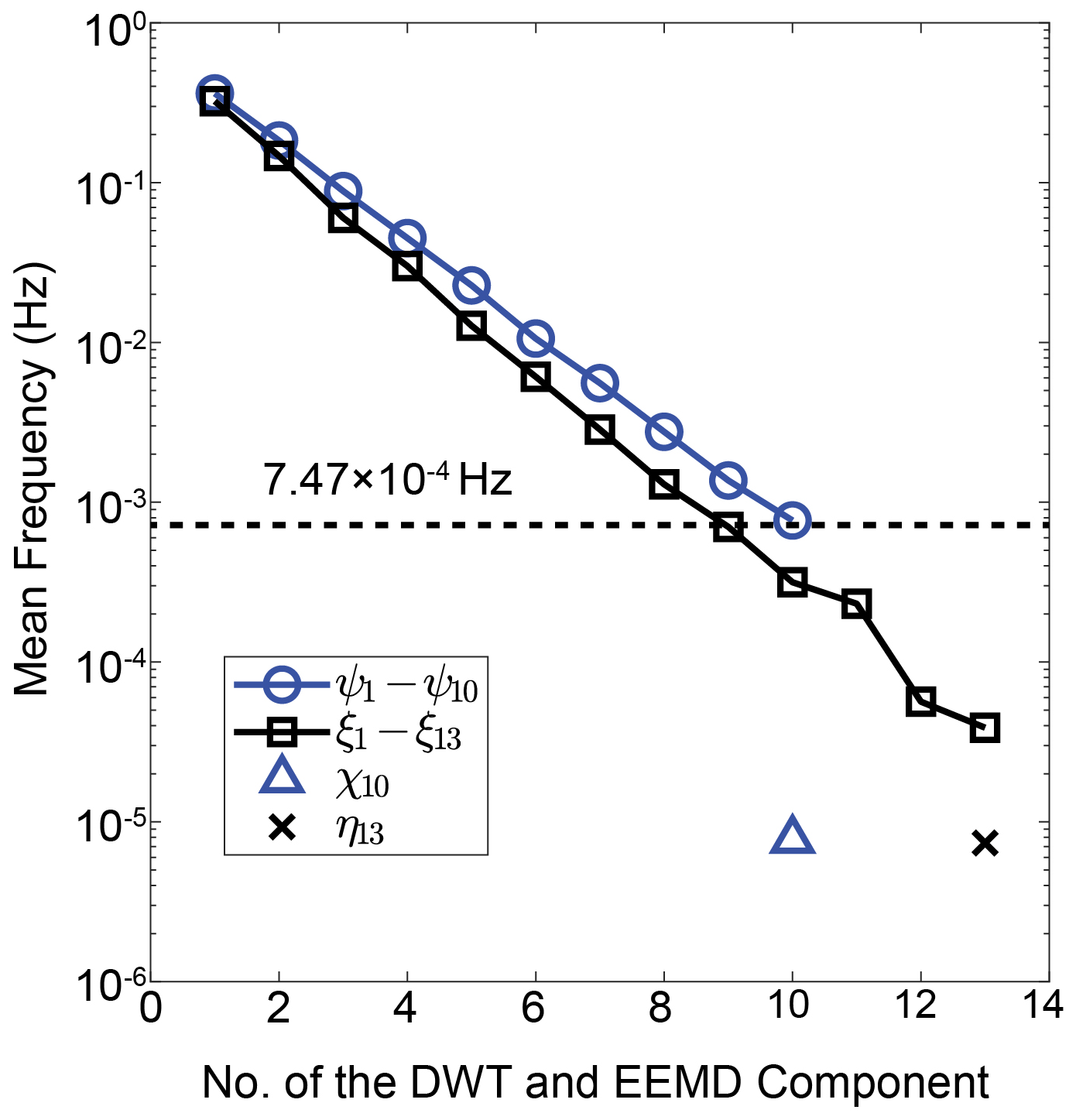
Figure 3The mean frequencies of DWT and EEMD components of E3 at 0.5 m height. The dashed line around the components ψ10 and ξ9 corresponds to the frequency of Hz.
In this study, the time-varying mean values can be alternatively defined as the sum of the last four EEMD components, ξ10 to ξ13, and the residual, η13, as follows:
According to the above definitions, the time-varying mean can be synchronously obtained by the DWT and EEMD methods. As an example, Fig. 2 shows the results of the DWT analysis (Fig. 2b) and EEMD decompositions (Fig. 2c) for an E field time series E in our field campaign. It can be seen that DWT and EEMD can properly capture a similar time-varying mean (Fig. 2a). This is because the EEMD is conceptually very similar to the DWT and thus behaves as a “wavelet-like” filter bank (Flandrin et al., 2004). As shown in Fig. 3, the frequencies contained in the DWT and EEMD components become progressively lower, where the mean frequencies of ψ10 and ξ9 are and Hz, respectively. The time-varying means (defined as the summation of the components below the dashed line in Fig. 3) χ10 and show very close mean frequencies of and Hz, respectively. We thus conclude that such definitions in Eqs. (3) and (5) can extract the time-varying mean over a certain scale of about Hz (below the dashed line in Fig. 3).
Since the 3D E fields are measured at five heights in our field campaign, we thus define the height-averaged time-varying mean values as follows:
in the range of 0.05 to 0.7 m height in order to normalize the E field data by a unified quantity. Furthermore, the E field data can be normalized as follows:
Additionally, to obtain the dimensionless vertical profile of the 3D E field, the height z should also be a dimensionless parameter. Here, the dimensionless height z∗ is defined as the ratio of height z to the mean saltation height during the whole observed dust storm, as follows:
where the saltation height zsalt during a certain time interval is defined as the height below which 99 % of the total mass flux is present and can be estimated based on the measured SPC-91 data (see Text S1 in the Supplement for more details).
Finally, the dimensionless vertical profiles of the 3D E field at different periods are fitted together by the third-order polynomial functions as follows:
where i=1, 2, and 3 correspond to the streamwise, spanwise, and vertical components, respectively.
For modelling steady state saltation, there are four primary processes including (1) particle saltating motion, (2) particle–particle midair collisions, (3) particle–bed collisions, and (4) particle–wind momentum coupling (Dupont et al., 2013; Kok and Renno, 2009). Also, the changes in both the momentum and electrical charge of each particle are taken into account in the particle–particle midair and particle–bed collisions. To avoid overestimating midair collisions in the 2D simulation (Carneiro et al., 2013), we simulate saltation trajectories in a real 3D domain. We use the discrete element method (DEM), which explicitly simulates each particle motion and describes the collisional forces between colliding particles encompassing normal and tangential components, to advance the evaluation of the effects of particle midair collisions. In a steady state saltation, the mean streamwise wind speed is statistically stationary and statistically 1D so that the mean wind flow can be modelled as a 1D field. In other words, in this study the numerical simulation is a 3D DEM model for particle motion but a 1D model for wind field. In the following subsections, we will describe each process in detail.
3.1 Size distribution of particle sample
Granular materials in natural phenomena, such as sand, aerosols, pulverized material, seeds of crops, etc., are made up of discrete particles with a wide range of sizes ranging from a few micrometres to millimetres. The log-normal distribution is generally used to approximate the size distribution of the sand sample (Marticorena and Bergametti, 1995; Dupont et al., 2013). Thus, the mass distribution function of a sand sample with two parameters, average diameter dm, and geometric standard deviation σp can be written as follows:
3.2 Equations of saltating particles motion
The total force acting on a saltating particle consists of three distinct interactions (Minier, 2016). The first one refers to the wind–particle interaction, which is dominated by the drag force with lifting forces, such as the Saffman force and Magnus force, being of secondary importance (Kok and Renno, 2009; Dupont et al., 2013). The second interaction refers to the particle–particle collisional forces or cohesion caused by physical contact between particles. Such interparticle collisional forces can be described as a function of the overlaps between the colliding particles. The third interaction refers to the forces due to external fields such as gravity and the E field. In this study, in addition to the drag force, we also take into account the Magnus force because of the remarkable rotation of saltating particles of the order of 100–1000 rev s−1 (Xie et al., 2007). The effects of electrostatic forces on particle motion, which are significant for large wind velocity (Schmidt et al., 1998; Zheng et al., 2003), are also taken into account. Consequently, the full governing equations of saltating particles can be written as follows:
where mp,i is the mass of the ith particle, up,i is the velocity of the particle, is the drag force, is the Magnus force, and are the normal and tangential collisional forces from the jth particle, respectively. g is the gravitational acceleration, and ζp,i is the charge-to-mass ratio of the sand particles and is altered during every collision (see Sect. 3.4). E is the 3D E field given by our measurements, Ii is the moment of inertia, ωp,i is the angular velocity of the particle, is the torque caused by the wind on the particle, and and are the tangential torque due to the tangential component of the particle collisional forces and the rolling resistance torque, respectively. The summation Σ represents the consideration of all particles that are in contact with the ith particle.
3.2.1 Wind-particle interactions
In the absence of saltating particles, the mean wind profile over a flat and homogeneous surface is well approximated by the log law (Anderson and Haff, 1988) as follows:
where um is the mean streamwise wind speed, z is the height above the surface, and u∗ is the friction velocity. κ≈0.41 is the von Kármán constant, and z0 is the aerodynamic roughness, which varies substantially from different flow conditions and can be approximately estimated as dm∕30 for the aeolian saltation on Earth (e.g. Kok et al., 2012; Carneiro et al., 2013). In the presence of saltation, due to the momentum coupling between the saltating particles and wind flow, the modified wind speed gradient can be written as follows for steady state and horizontally homogeneous saltation (e.g. Kok and Renno, 2009; Pähtz et al., 2015):
where ρa is the air density, and τp(z) is the particle momentum flux and can be numerically determined by (Carneiro et al., 2013; Shao, 2008) the following:
with Lx, Ly, and Δz being the streamwise- and spanwise-width of the computational domain and the vertical grid size, respectively. up,i and wp,i are the streamwise and vertical components of the particle velocity. The summation in Eq. (14) is performed on the particles located in the range of . Once the saltating particle trajectories are known, the wind profile can be determined through integrating Eq. (13) with the no-slip boundary condition um=0 at z=z0.
Since sand particles are much heavier than the air and are far smaller than the Kolmogorov scales, the drag force is the dominant force affecting the particle motion, which is expressed by (Anderson and Haff, 1991) the following:
where dp is the diameter of the particle, Cd is the drag coefficient, and is the particle-to-wind relative velocity. The drag coefficient Cd is a function of the particle Reynolds number, , where μ is the dynamic viscosity of the air. We calculate the drag coefficient with an empirical relation , which is applicable to the regimes from Stokes flow Rep≪1 to high Reynolds number turbulent flow (Cheng, 1997).
Additionally, we also account for the effects of particle rotation on particle motion using the Magnus force expressed as follows (White and Schulz, 1977; Anderson and Hallet, 1986; Loth, 2008):
where Cm is a normalized spin lift coefficient, depending on the particle Reynolds number and the circumferential speed of the particle. The torque acting on a particle caused by wind flow is calculated from (Anderson and Hallet, 1986; Shao, 2008; Kok and Renno, 2009) the following:
3.2.2 Particle–particle midair collisions
Under moderate conditions, saltation is a dilute flow in which the particle–particle collisions are negligible. However, as wind velocity increases, midair collisions become increasingly pronounced, especially in the near-surface region (Sørensen and McEwan, 1996). Previous studies found that the probability of midair collisions of saltating particles almost increased linearly with wind speed (Huang et al., 2007), and such collisions indeed enhanced the total mass flux substantially (Carneiro et al., 2013). For spherical particles, one of the most commonly used collisional force models is the non-linear viscoelastic model, consisting of two components, i.e. elastic and viscous forces (Haff and Anderson, 1993; Brilliantov et al., 1996; Silbert et al., 2001; Tuley et al., 2010).
Considering that two spherical particles i and j, with diameters di and dj and position vectors xi and xj, are in contact with each other, the relative velocity vij at the contact point and its normal and tangential components, and , are respectively defined as follows (Silbert et al., 2001; Norouzi et al., 2016):
where is the unit vector in the direction from the centre of particle i point towards the centre of particle j. Supposing that these colliding particles have identical mechanical properties to Young's modulus Y, shear modulus G, and Poisson's ratio ν, the normal collisional force can thus be calculated by (Brilliantov et al., 1996; Silbert et al., 2001) the following:
where is the equivalent Young's modulus, is the normal overlap, is the equivalent particle mass, is the normal contact stiffness, is the equivalent particle radius, and β is related to the coefficient of restitution en by the relationship ; and . The first term on the right-hand side of Eq. (19) represents the elastic force described by Hertz's theory, and the second term represents the viscous force reflecting the inelastic collisions between sand particles. Similarly, the tangential collisional force, which is limited by the Coulomb friction, is given as follows (Brilliantov et al., 1996; Silbert et al., 2001):
where is the equivalent shear modulus, δt is the tangential overlap, is the tangential unit vector at the contact point, is the tangential stiffness, , and γs is the coefficient of static friction. The torque on the ith particle arising from the jth particle collisional force is defined as (Haff and Anderson, 1993) the follows:
To account for the significant rolling friction, we apply a rolling resistance torque (Ai et al., 2011) as follows:
on each colliding particle, where μr is the coefficient of rolling friction, and is the unit vector of relative angular velocity.
3.3 Particle–bed collisions
As a saltating particle collides with the sand bed, it not only has a chance to rebound but may also eject several particles from the sand bed. For simplicity, we use a probabilistic representation, termed as the “splash function”, to describe the particle–bed interactions quantitatively (Shao, 2008; Kok et al., 2012). Currently, the splash function is primarily characterized by wind-tunnel and numerical simulations (e.g. Anderson and Haff, 1991; Haff and Anderson, 1993; Rice et al., 1996; Huang et al., 2017). The rebounding probability of a saltating particle colliding with the sand bed is approximately (Anderson and Haff, 1991) the following:
where vimp is the impact speed of the saltating particle. The kinetic energy of the rebounding particles is taken as 0.45±0.22 of the impact particle (Kok and Renno, 2009). The rebounding angles θ and φ, as depicted in Fig. 4a, obey an exponential distribution with a mean value of 40∘, i.e. , and a normal distribution with the parameters 0±10∘, i.e. φ∼N(0∘,10∘), respectively (Kok and Renno, 2009; Dupont et al., 2013).
It is reasonable to assume that the number of ejected particles depends on the impact speed and its cross-sectional area. Thus, the number of ejected particles from the kth particle bin is (Kok and Renno, 2009) as follows:
where m is a reference diameter, Dimp and are the diameter of the impact and ejected particles, respectively, and pk is the mass fraction of the kth particle bin. The speed of the ejected particles obeys an exponential distribution, with the mean value taken as (Kok and Renno, 2009). Similar to the rebound process, the ejected angles θ and φ are assumed to be and .
3.4 Particle charge exchanges
In this study, the calculation of the charge transfer between sand particle collisions is based on the asymmetric contact model, assuming that the electrons trapped in high-energy states on one particle surface can relax on the other particle surface (Kok and Lacks, 2009; Hu et al., 2012). Thus, the net increment of the charge of particle i after colliding with particle j, Δqij, can be determined by the following:
where C is the elementary charge, is the density of the electrons trapped in the high energy states on the surface of particle i (assuming that all particles have an identical initial value, i.e., ), which is modified as follows (Zhang et al., 2013):
due to collisions between particle i and j. Si is the particle contact area, which can be approximately calculated as a line integral along the contact path Li of particle i as follows:
where dli is the differential of the contact length. In general, when two particles are in contact with each other, the relative sliding motion between the two particles results in two unequal contact areas, Si and Sj, thus producing a net charge transfer Δqij between the two particles. If the particle's net electrical charge is known, its charge-to-mass ratio can be easily determined.
3.5 Particle-phase statistics
Similar to particle momentum flux (i.e. Eq. 14), the particle horizontal mass flux q, total mass flux Q, mean particle mass concentration mc (Carneiro et al., 2013; Dupont et al., 2013), and mean particle charge-to-mass ratio 〈ζp〉 can be numerically determined by the following:
where the summation ∑ is performed over the saltating particles located in the range of for q, mc, and 〈ζp〉, but it is performed over all saltating particles for Q. Here, we define the 〈ζp〉 as the ratio of charge flux and mass flux in the range of .
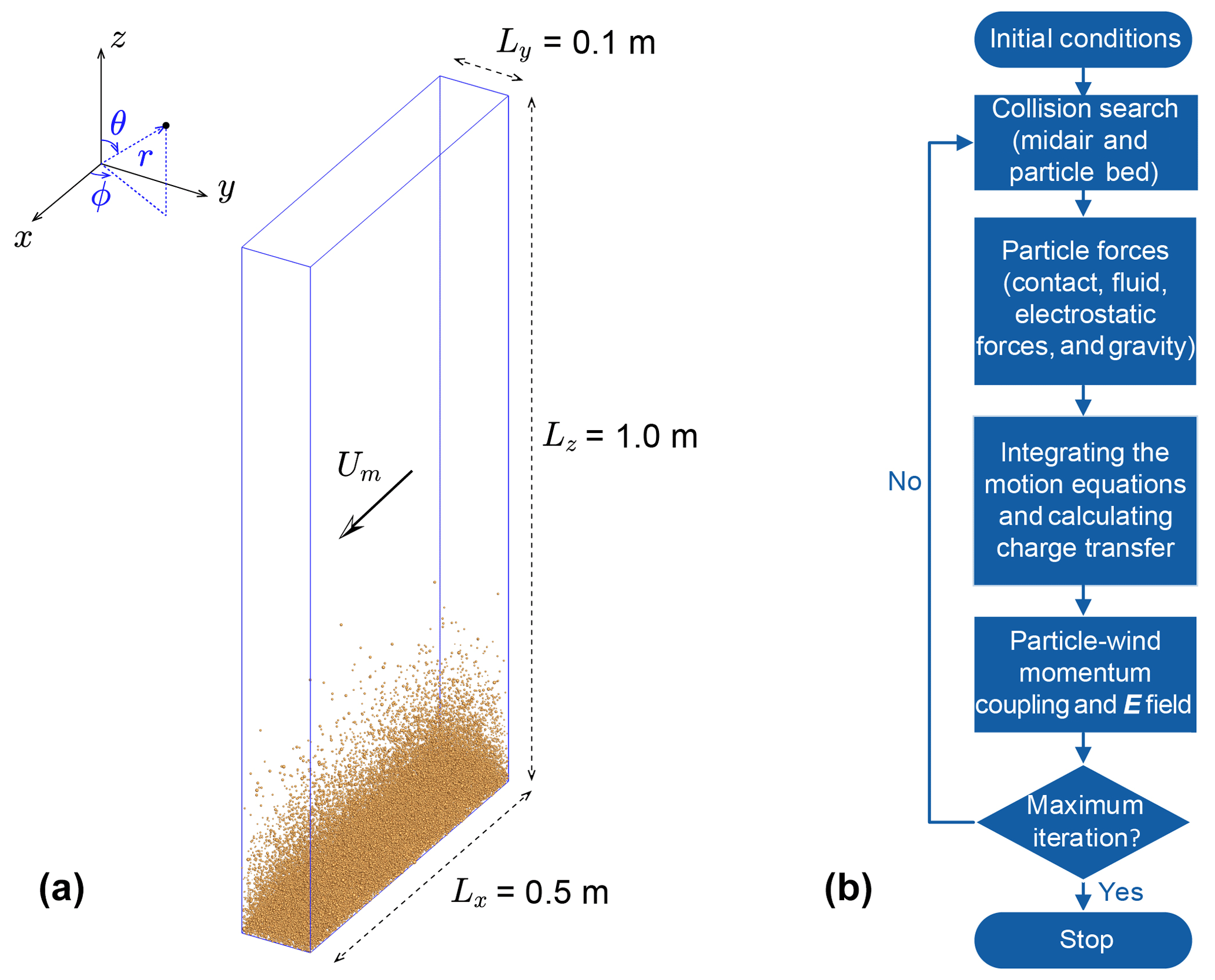
Figure 4A schematic illustration of the DEM simulation of saltation and the numerical algorithm of the saltation model. (a) A 3D view of the simulated wind-blown sand at the steady state, where the wind shear velocity is m s−1, average sand diameter is dm=228 µm, and geometric standard deviation is σp=exp (0.3). Both the Cartesian and spherical coordinates are shown in the inset. (b) This flow chart shows the scheme for simulating the saltation according to the following steps by implementing the DEM with particle triboelectric charging: initial conditions, collision search, particle forces, integrating motion equations and calculating charge transfer, particle–wind momentum coupling and evaluating the E field, and, finally, repeating these executed steps until the maximum iteration steps are reached.
3.6 Model implementation
We consider polydisperse soft-spherical sand particles to have a log-normal mass distribution in a 3D computational domain (as shown in Fig. 4a), with periodic boundary conditions in the x and y directions. Here, the upper boundary is set to be high enough so that the particle escapes from the upper boundary can be avoided. To reduce the computational cost, the spanwise dimension is chosen as Ly=0.1, since the saltating particles are mainly moving along the streamwise direction.
As shown in Fig. 4b, the model is initiated by randomly releasing 100 uncharged particles within the region below 0.3 m, and then, these released particles begin to move under the action of the initial log-law wind flow, triggering saltation through a series of particle–bed collisions. We use cell-based collision-searching algorithms, which perform a collision search for particles located in the target cell and its neighbouring cells, to find the midair colliding pairs. The random processes, particle–bed collisions described previously, are simulated using a general method called the inverse transformation. The particle motion and wind flow equations are integrated by predictor-corrector method AB3-AM4; that is, the third-order Adams–Bashforth method is used to perform the prediction and fourth-order Adams–Moulton method is used to perform the correction. One of the main advantages of using such a multi-step integration method is that the accuracy of the results is not sensitive to the detection of exact moments of collision (Tuley et al., 2010). The charge transfer between the colliding pairs is caused by their asymmetric contact and can be determined by Eqs. (25)–(27). When calculating the particle–bed charge transfer, the bed is regarded as an infinite plane. According to the law of charge conservation, the surface charge density of the infinite bed plane and the newly ejected particles, σ, is (Kok and Renno, 2008; Zhang et al., 2014) as follows:
where ρc is the space charge density. To model pure saltation, the E field is calculated by Gauss's law (e.g. Zhang et al., 2014). To model saltation during dust storms, the 3D E field is directly formulated by Eq. (9), based on our field measurements, as mentioned above. The variables used in this study are listed and described in Table 1.
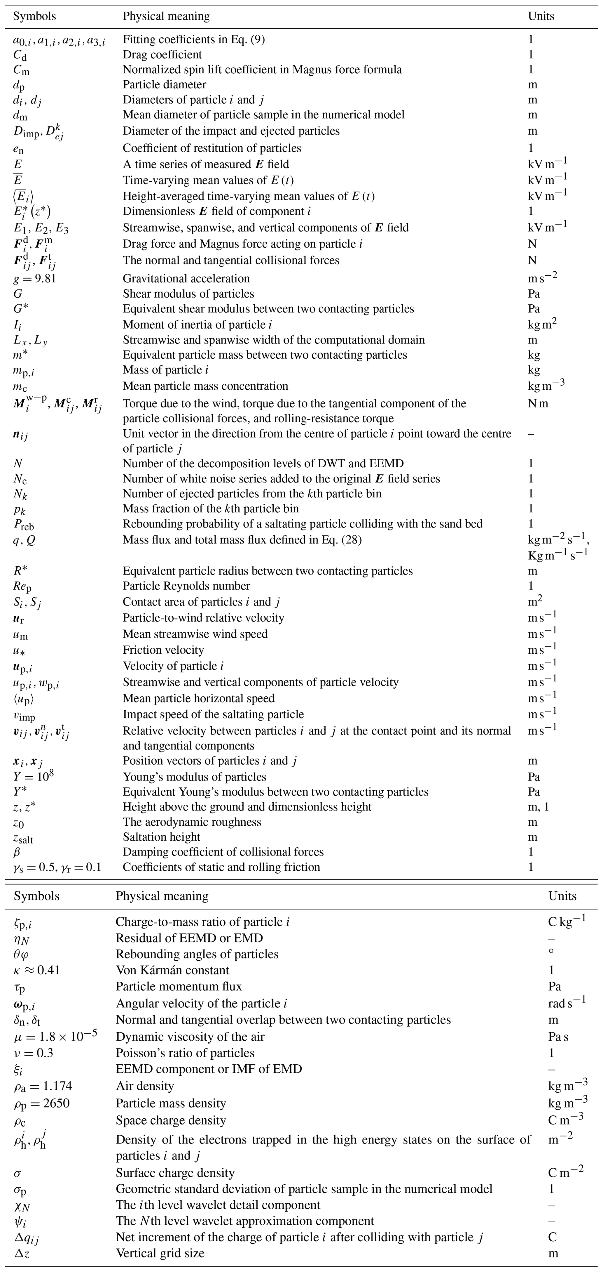

Figure 5Measured data during a dust storm occurring on 6 May 2014 at the QLOA site. Panels (a)–(b) show the measured time series of the streamwise wind speed, with um at 0.7 m and the number of saltating particle N at 0.15 m. Panels (c)–(g) correspond to the streamwise E field E1 (grey lines), spanwise E field E2 (black lines), and vertical E field E3 (blue lines) at 0.05, 0.15, 0.3, 0.5, and 0.7 m height, respectively. Unfortunately, owing to the interruption in the power supply, the 3D E field data were not recorded before ∼12:30 UTC+8, as represented by the shading in panels (c)–(g). The dashed box denotes the relatively stationary period of the observed dust storm because, during this period, the time-varying means of all quantities (such as χ10, depicted by the solid white lines in panels a–g and dashed red lines in panels h–n) do not vary notably as time varies (Bendat and Piersol, 2011), as shown in panels (h)–(n).
4.1 Vertical profiles of 3D E field
On 6 May 2014, field measurements began at ∼ 12:00 UTC+8 due to the limited power supply by solar panels. As shown in Fig. 5, although the early stage of the dust storm has not been observed completely, we successfully recorded data of about 8 h, which is substantial enough to reveal the pattern of the 3D E field. From Fig. 5, it can be seen that the relative magnitudes of E1, E2, and E3 vary with height. For example, the magnitude of E3 is larger than that of E1 and E2 at 0.15 m height (Fig. 5k) but is smaller than that of E1 and E2 at 0.7 m height (Fig. 5n). The vertical profiles of the normalized streamwise, spanwise, and vertical components of the E field are shown in Fig. 6a–c, respectively. To the best of our knowledge, these data are the first measured 3D E field data in the sub-metre layer during dust storms. Numerous studies showed that the vertical component of the E field in pure saltation decreased with increasing height (e.g. Schmidt et al., 1998; Kok and Renno, 2008; Zhang et al., 2014). Interestingly, Fig. 6a–c show that, during dust storms, all normalized components, from to , decrease monotonically as height increases in the saltation layer (i.e. ), similar to the pattern of the vertical component in pure saltation.

Figure 6Vertical profiles of the normalized 3D E field. Panels (a)–(c), in turn, correspond to the vertical profiles of , , and of the observed dust storm. Squares and circles denote the DWT mean and EEMD mean values of the normalized E field data, respectively. Error bars are standard deviations. Lines denote the robust linear least-squares fitting of the normalized E field data obtained by the DWT and EEMD method using third-order polynomials (with R2 of 0.97, 0.80, and 0.67, respectively), where the shaded areas denote 95 % confidence bounds.
Table 2Fitting coefficients of the third-order polynomial curves in Fig. 6.
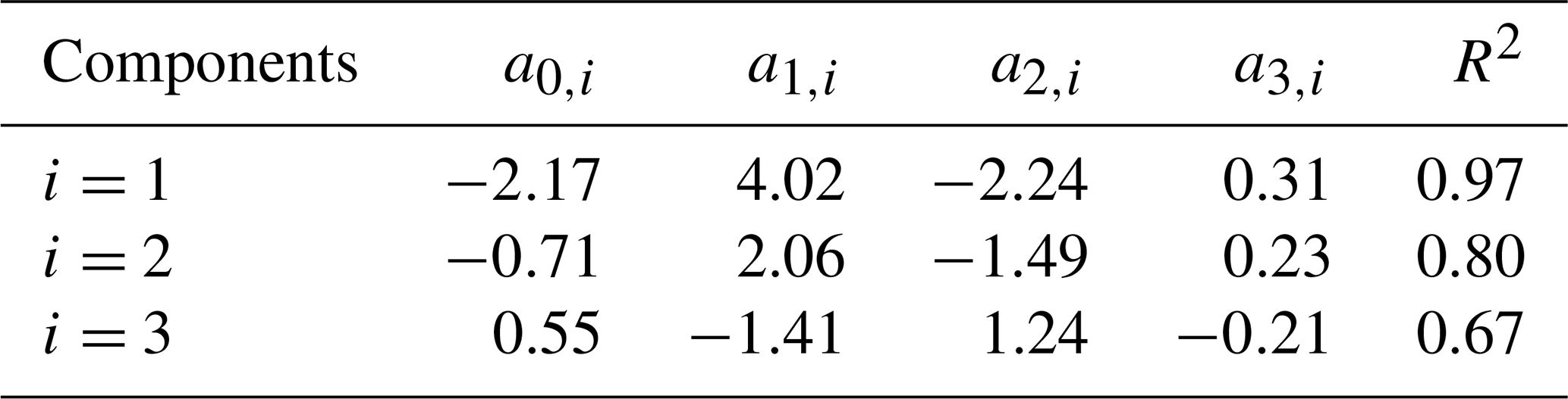
As shown in Fig. 6a–c, in different periods, each component of the normalized 3D E field roughly collapses on a single third-order polynomial curve (with R2=0.67–0.97; see Table 2 for details). This suggests that, during dust storms, the 3D E field in the sub-metre layer can be characterized as , where represents the pattern of the dimensionless E field vertical profile (formulated by Eq. 9), and represents the height-averaged time-varying mean defined in Eq. (6). It is worth noting that the E field pattern and their intensities are strongly dependent on the saltation conditions, such as dust mass loading, temperature, relative humidity (RH), etc. For example, at a given ambient temperature and RH, the mean E field intensities increase linearly with dust mass loading (e.g. Esposito et al., 2016; Zhang et al., 2017). In addition, both and could vary from event to event, and among them, the saltation conditions are quite different. So far, a quantitative representation of is challenging due to its high complexity, and thus we regard it as a basic parameter in the following sections for exploring the effects of 3D E field on saltation. The fitting results of Eq. (9) are listed in Table 2, with the coefficients rounded to two decimals. The formulations of the 3D E field can be readily substituted into the numerical model (i.e. Eq. 11a).
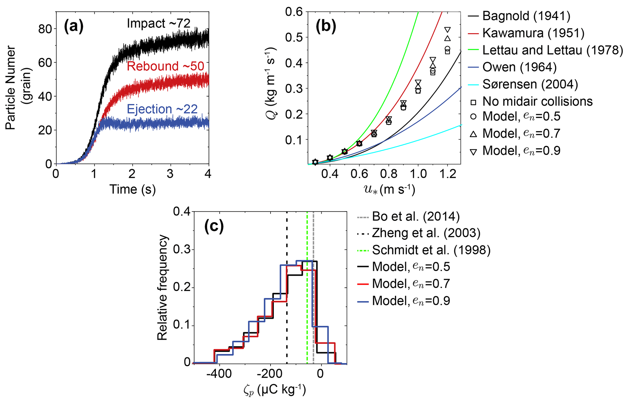
Figure 7Verification of the steady state numerical model in the case of pure saltation. That is, only the vertical E field needs to be considered as it is produced by the charged saltating particles. (a) The number of the impacting, rebounding, and ejected particles within each period of 10−4 s, where m s−1, dm=228 µm, and σp=exp (0.3). (b) Comparison of the simulated total mass flux with the most commonly used semiempirical saltation mass flux equations (Bagnold, 1941; Kawamura, 1951; Lettau and Lettau, 1978; Owen, 1964; Sørensen, 2004), where dm=228 µm and σp=exp (0.3). (c) Comparison of the simulated charge-to-mass ratio distribution in the range of 0.07–0.09 m height, with the measured mean charge-to-mass ratio in the range of 0.06–0.1 m height (Zheng et al., 2003) at 0.05 m height (Schmidt et al., 1998) and 0.08 m height (Bo et al., 2014). Here, m−2 is determined by calibrating the model with measurements. m s−1, dm=203 µm, and σp=exp (0.33) are estimated from Zheng et al. (2003).
4.2 Effects of particle–particle midair collisions on saltation
Before quantifying the effects of the 3D E field on saltation by our numerical model, we draw a comparison of several key physical quantities between the simulated results and measurements in the case of pure saltation in order to ensure the convergence and validity of our numerical code, as shown in Fig. 7a–c. It is clearly shown that the saltation eventually reaches a dynamic steady state after ∼4 s. The number of the impacting particles (∼72 grains) is equal to the sum of the rebounding (∼50 grains) and the ejected particles (∼22 grains) during the time interval of 10−4 s. At the steady state, each impacting particle, on average, produces a single saltating particle, either by rebound or by ejection. As shown in Fig. 7b, the total mass flux is well predicted by our numerical model, and midair collisions enhance the total mass flux dramatically, especially for less particle-viscous dissipation (i.e. large en) and large friction velocity. As in previous studies (e.g. Haff and Anderson, 1993; Carneiro et al., 2013), the selected en is larger than 0.5 since the en of quartz sand particles has been expected to lie in the range of ∼0.5–0.6 (Haff and Anderson, 1993; Kok et al., 2012). Also, the predicted charge-to-mass ratios of saltating particles are widely distributed from −400 to +60 µC kg−1, consistent with the previous measurements of the charge-to-mass ratio in pure saltation (Schmidt et al., 1998; Zheng et al., 2003; Bo et al., 2014). To our knowledge, so far there are no actual measurements of charge on a single sand particle in dust events. In the case of Fig. 7c, the magnitude of the simulated mean charge-to-mass ratio is around 100 µC kg−1, corresponding to a mean charge of C per particle. This is in accordance with the empirical values of 10−14–10−12 C per particle (Merrison, 2012).
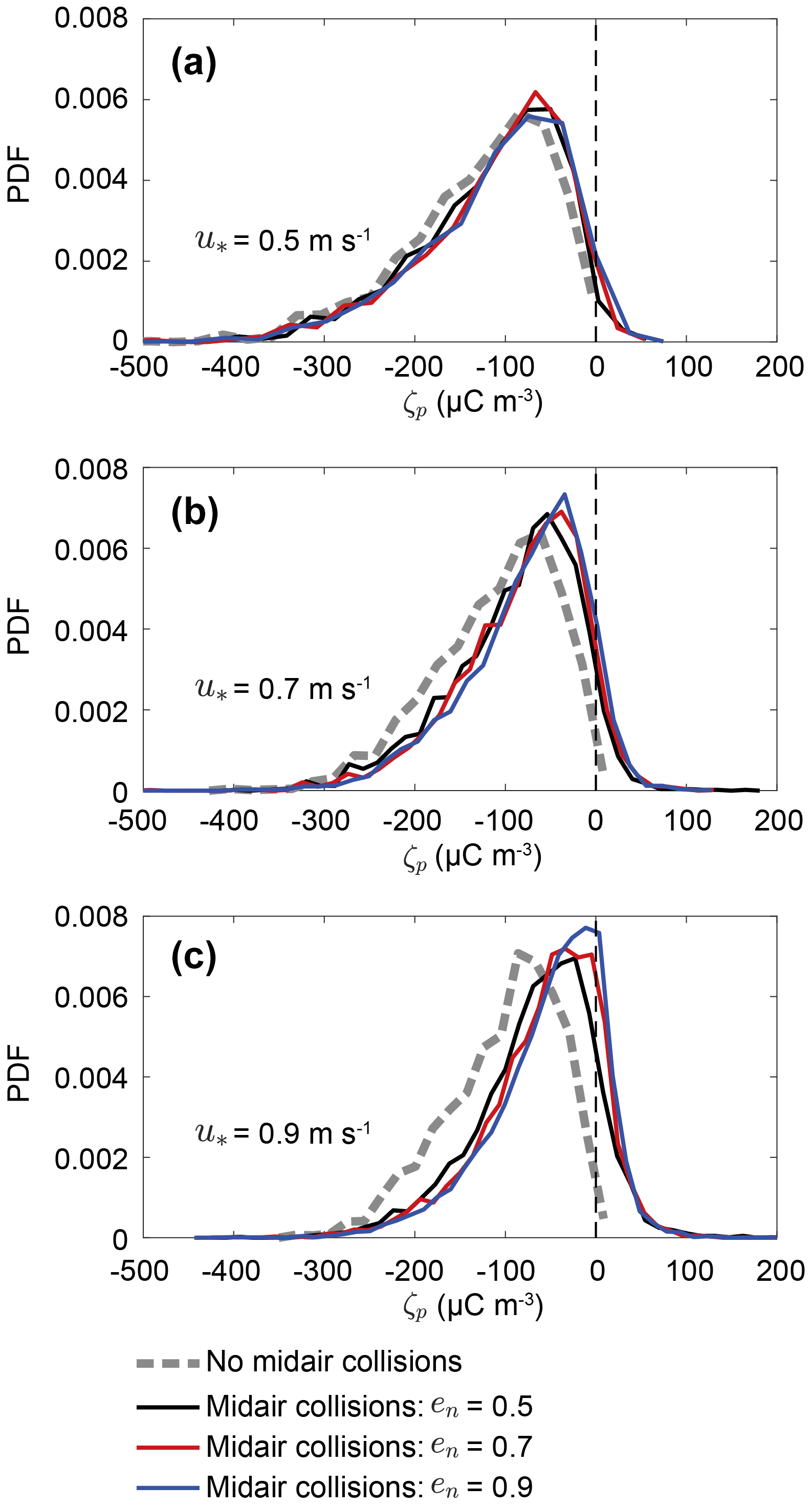
Figure 8Effects of midair collisions on the probability density function (PDF) of the charge-to-mass ratio of saltating particles for various wind velocities of (a) m s−1, (b) m s−1, and (c) m s−1, where dm=203 µm, σp=exp (0.33), and m−2.
In addition to affecting sand transport, midair collisions also affect charge exchanges between saltating particles. When considering midair collisions, the charge-to-mass ratio distribution shifts slightly towards zero as the wind velocity increases, as shown in Fig. 8a–c. As the wind speed increases, the difference in the charge-to-mass ratio distribution between the cases with and without midair collisions is increasingly notable. This is because the probability of midair collisions becomes more significant for larger wind speed (Sørensen and McEwan, 1996; Huang et al., 2007).
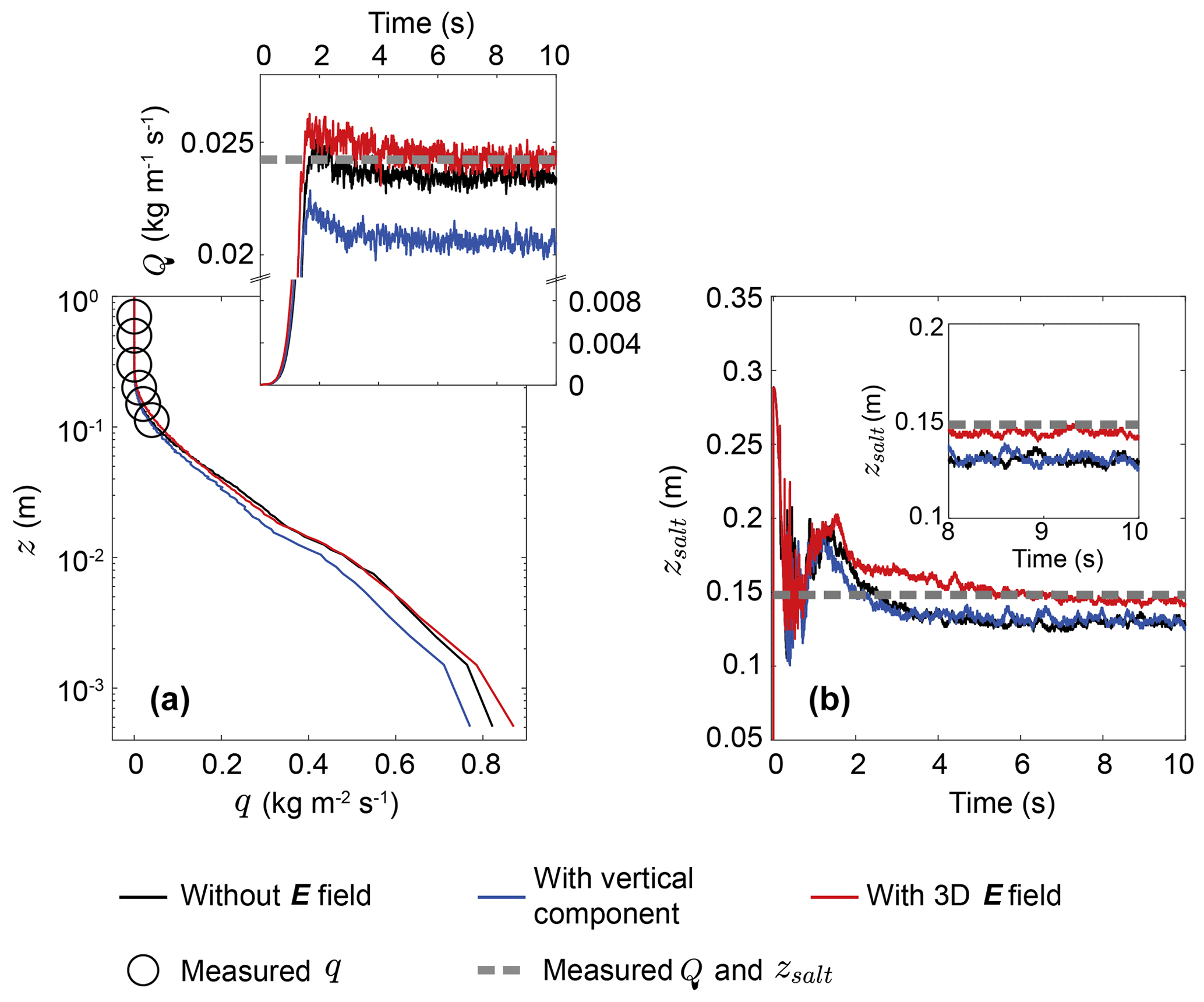
Figure 9Comparison of the simulated mass flux q and total mass flux Q (a) and saltation height zsalt (b) with our measurements in the relatively stationary period of the observed dust storm (shaded areas in Figs. 4 and S3), where m s−1, dm=200 µm, σp=exp (0.42), m−2, and en=0.7. (a) Circles are the measured mean mass flux, the dashed line denotes the estimated mean total mass flux, and lines denote the simulated results. (b) Dashed lines denote the estimated saltation height based on our measurements, and the lines denote simulated results. Inset shows the same data from 8 to 10 s. The uncertainty analysis of the measured or estimated results can be found in Text S1 in the Supplement.

Figure 10Vertical profiles of the particle mass concentration mc and mean particle horizontal speed 〈up〉 for different cases, where 〈up〉 is calculated as the arithmetic mean of the particle horizontal speed located in the range of . Insets show the same data and emphasize the local information. In these cases, m s−1, dm=200 µm, σp=exp (0.42), m−2, and en=0.7.
4.3 Effects of 3D E field on saltation
By substituting the formulations of the 3D E field (i.e. , ) into our model (i.e. Eq. 11a), we then properly evaluated the effects of the 3D E field on saltation during storms. As shown in Fig. 9a, compared to the case without E field, the vertical component of the E field (i.e. 1D E field) inhibits mass flux, which is in agreement with previous studies (Kok and Renno, 2008; Zheng et al., 2003). However, the mass flux is enhanced by the 3D E field, causing the simulated value closer to our measured data. Such an enhancement in the mass flux by the 3D E field can be qualitatively explained by the considerable enhancements in mc below a ∼0.02 m height (Fig. 10a) and 〈up〉 in the range from 0.01 to 0.1 m height (Fig. 10b) due to the streamwise and spanwise E field components. Meanwhile, although the saltation height is not sensitive to the E field vertical component, the 3D E field enhances the saltation height significantly and, therefore, makes the numerical prediction more accurate (Fig. 9b). This is because, when considering the E field vertical component, the mass flux profile is very similar to the case of no E field consideration (Figs. 9a and 10). In contrast, the 3D E field distorts the mass flux profile (in addition to mc and 〈up〉) and, thus, alters saltation height significantly (Figs. 9a and 10).

Figure 11Effects of the density of charged species on saltation for two different height-averaged time-varying mean levels (i.e. , ). (a) The mean charge-to-mass ratio 〈ζp〉 (in the range from 0.07 to 0.09 m height) as a function of ranging from 1014 to 1020 m−2 (e.g. Kok and Lacks, 2009). (b) Percent increase in the total mass flux Q as a function of . (c) Percent increase in the saltation height zsalt as a function of . The squares correspond to the height-averaged time-varying mean in the stationary stage of the observed dust storm (shaded areas in Fig. S5 in the Supplement). In these cases, en=0.7.
Additionally, we also explore how the key parameter, the density of charged species , affects saltation, as shown in Fig. 11a–c. Since the height-averaged time-varying mean is strongly dependent on the ambient conditions, such as temperature and RH, the height-averaged time-varying mean is set at two different levels. The predicted results show that, at each height-averaged time-varying mean level, the magnitude of the mean charge-to-mass ratio increases with increasing and then reaches a relative equilibrium value at approximately m−2 (Fig. 11a), thus leading to the constant enhancement of total mass flux Q and saltation height zsalt (Fig. 11b and c). From Eqs. (25)–(26), it can be seen that the net charge transfer Δqij is proportional to the initial density , so that 〈ζp〉 increases rapidly with increasing for small . However, for larger , Δqij is no longer proportional to because, in this case, the difference in the number of trapped electrons between two colliding particles (i.e. ) has the same value, and is not the key parameter for determining the mean charge-to-mass ratio (Kok and Lacks, 2009). Figure 11c shows a peak of increase in zsalt at of about 1016–1017 m−2 because 〈ζp〉 also exhibits a peak in the same range of . In addition, the peak is more apparent in Fig. 11c. This is because zsalt is very sensitive to the mass flux profile. A little change in mass flux profile can lead to an apparent change in zsalt (see Text S1 in the Supplement). For the larger height-averaged time-varying mean, the enhancements in the total mass flux Q and saltation height zsalt could exceed 20 % and 15 %, respectively.
5.1 Field measurements of 3D E field in the sub-metre layer
To determine the effects of particle triboelectric charging on saltation precisely, 3D E field measurements in the saltation layer (i.e. sub-metre above the ground) are required. Although the E field measurements, such as those by Rudge (1913), Kamra (1972), Williams et al. (2009), Bo and Zheng (2013), Esposito et al. (2016), and Zhang et al. (2017), in dust storms are numerous, the 3D E field in the sub-metre layer has not been studied so far. This is because the traditional atmospheric E field sensors, such as the CS110 sensor manufactured by Campbell Scientific, Inc., have dimensions of cm3 (e.g. Esposito et al., 2016; Yair et al., 2016), which is too large compared to the height of saltation layer. Thus, it will lead to significant disturbances in the ambient E field. Fortunately, the diameter of the VREFM sensor developed by Lanzhou University is only 2.5 cm and, thus, could considerably eliminate the E field disturbances (Zheng, 2013; Zhang et al., 2017). In this study, using the VREFM sensors, we have measured and characterized the 3D E field from 0.05 to 0.7 m height during dust storms, which can provide valuable data for investigating the mechanisms of particle triboelectric charging in saltation.
In E field data analysis, the E field is normalized by its time-varying mean over a certain timescale, which can be extracted by the DWT and EEMD methods with negligible end effects and mode mixing (Percival and Walden, 2000; Wu and Huang, 2009). At the same time, since the saltation height zsalt slightly varies with time (i.e. 0.172±0.0343 m; see Fig. S3 in the Supplement), the height z above the ground is normalized by the mean saltation height . Note that we calculate the saltation height and mass flux over every 30 min time interval because a sufficiently long period is needed to capture all scales of turbulence (Sherman and Li, 2012; Martin and Kok, 2017). The 3D E field pattern is finally characterized as third-order polynomials, but it is only valid in the range that is not too far beyond the measurement points. Additionally, the 3D E field pattern of dust storms may vary from event to event because it is strongly related to the driving mechanisms of dust storms, such as monsoon winds, squall lines, and thunderstorms (Shao, 2008), and ambient conditions, such as temperature and relative humidity (Esposito et al., 2016; Zhang and Zheng, 2018). Although the 3D E field pattern revealed in this study may not be a universal feature, the proposed E field data analysis method can be easily applied to other cases.
5.2 Potential mechanisms for generating intense horizontal E field in dust storms
Like many previous studies, the E field can be simplified to 1D (i.e. vertical component) in pure saltation (e.g. Kok and Renno, 2008) since, in such cases, the magnitude of the streamwise and spanwise components is much less than that of the vertical component (Zhang et al., 2014). However, during dust storms, the magnitudes of the streamwise and spanwise components of the E field are near the magnitude of the vertical component, as mentioned previously. The E field is therefore 3D in dust storms. In contrast to the vertical component, which is closely related to the total mass loading (Williams et al., 2009; Esposito et al., 2016), the intense streamwise and spanwise components of the E field in dust storms may be aerodynamically created by the unsteady wind flows (Zhang et al., 2014) and turbulent fluctuations (Cimarelli et al., 2014; Di Renzo and Urzay, 2018). It is well known that a dust storm is a polydisperse (having dust particles with diameters from <10 to ∼500 µm), particle-laden turbulent flow at a very high Reynolds number (up to ∼108). The wind flow in dust storms is certainly unsteady and random. Numerical simulation by Zhang et al. (2014) showed that the unsteady incoming flow could lead to the non-uniform transport of charged particles in the streamwise direction and, thus, result in fluctuating streamwise and vertical E fields. In addition to unsteadiness, recent direct numerical simulations (Di Renzo and Urzay, 2018) and laboratory experiments (Cimarelli et al., 2014) of particle-laden turbulent flows demonstrated that the generation of the 3D E field could be caused by turbulent fluctuations. That is, the negatively charged small particles are affected by local turbulence and tend to accumulate in the interstitial regions between vortices, while the positively charged larger particles are unresponsive to turbulent fluctuations and are more uniformly distributed than the smaller ones (Cimarelli et al., 2014; Di Renzo and Urzay, 2018). We thus reasonably expect that the negatively charged finer dust particles (<10 µm) accumulate in specific regions, while the positively charged coarser sand particles (>100 µm) are more uniformly distributed due to their large inertia. Note that numerous studies found that larger and smaller particles tended to charge positively and negatively, respectively (e.g. Zheng et al., 2003; Forward et al., 2009; Kok and Lacks, 2009), but a few studies reported the opposite polarity when particle–wall interactions were present (e.g. Mehrani et al., 2005; Sowinski et al., 2010). Doubtless, such a charge segregation could produce a 3D E field (e.g. Di Renzo and Urzay, 2018). More recently, using the 3D E field data collected in an atmospheric surface layer observation array, Zhang and Zhou (2020) established an inversion method, based on Tikhonov regularization, to reconstruct the electrical structures of dust storms, and the results demonstrated the turbulence-driven charge segregation and the 3D E field pattern of dust storms. To sum up, the generating mechanisms responsible for the streamwise and spanwise E fields in dust storms are probably due to the charge segregation caused by unsteady wind flows and turbulent fluctuations.
Additionally, one possible explanation for the intense streamwise and spanwise E fields is that large- and very large-scale motions exist in atmospheric surface flows, leading to a large-extent charge segregation in the streamwise and spanwise directions. In atmospheric surface layer flows, the largest vortices or coherent motions of the wind flows are found to be compared to the boundary layer thickness (∼60–200 m; Kunkel and Marusic, 2006; Hutchins et al., 2012). This may lead to a phenomenon in which the charged particles are more non-uniformly distributed (over a larger spatial scale) in the streamwise and spanwise directions than in the vertical direction. Accordingly, the intensities of the streamwise and spanwise E fields are probably larger than those of the vertical E field.
5.3 Particle–particle triboelectric charging resolved model
Although most physical mechanisms, such as asymmetric contact, polarization by external E fields, statistical variations in material properties, and shift of aqueous ions, are responsible for particle triboelectric charging, contact or triboelectric charging is the primary mechanism (e.g. Lacks and Sankaran, 2011; Zheng, 2013; Harrison et al., 2016). In the previous model, however, the charge-to-mass ratios of the saltating particles are either assumed to be a constant value (e.g. Schmidt et al., 1998; Zheng et al., 2003; Zhang et al., 2014) or are not accounted for in the particle–particle midair collisions (e.g. Kok and Renno, 2008). In this study, by using DEM together with an asymmetric contact electrification model, we account for the particle–particle triboelectric charging during midair collisions in saltation. The DEM implemented by cell-based algorithms is effective for detecting and evaluating most of the particle–particle midair collisional dynamics (Norouzi et al., 2016). Meanwhile, the charge transfer between colliding particles can be determined by Eqs. (25) and (26). Compared to the previous studies (e.g. Kok and Lacks, 2009), the main innovation of this model is that the comprehensive consideration of the particle collisional dynamics affecting particle charge transfer is involved. In summary, the present model is a particle–particle midair collision resolved model, and the predicted charge-to-mass ratio agrees well with the published measurement data (see Fig. 7c). These findings indicate that midair collisions in saltation are important, both in momentum and charge exchanges.
One limitation of our model is that the effects of turbulent fluctuations on particle charging and dynamics are not explicitly accounted for. In actual conditions, saltation is unsteady and inhomogeneous at small scales, and the wind flow is mathematically described by the continuity and Navier–Stokes equations. However, in many cases, wind flow is statistically steady and homogeneous over a typical timescale of 10 min (Durán et al., 2011; Kok et al., 2012). For example, in the relatively stationary period in Fig. 5, all long period-averaged statistics become independent of time. In this case, the governing equations of the wind flow can be reduced to a simple model described by equation Eq. (13). There is no doubt that 3D turbulent fluctuations could affect particle charging and dynamics considerably (e.g. Cimarelli et al., 2014; Dupont et al., 2013). Further work is therefore needed to incorporate turbulence into the numerical model.
5.4 Implications for evaluating particle triboelectric charging in dust events
It is generally accepted that the E field could considerably affect the lifting and transport of sand particles. As in the findings of previous 1D E field models (e.g. Kok and Renno, 2008), the E field has been proven to inhibit sand transport in our model when considering the vertical component of the E field alone. It is worth noting that, unlike the natural 1D E field produced by the charged sand particles, the artificial 1D E field may enhance sand transport in pure saltation when it is oriented opposite to the natural 1D E field. For example, Rasmussen et al. (2009) found that sand mass flux in pure saltation was significantly enhanced when a downward-pointing external E field (opposite to the direction of actual vertical E field) with a magnitude of 270 kV m−1 was applied. In contrast to the 1D E field, our model further shows that the real 3D E field in dust storms enhances sand transport substantially, consistent with a recent measurement by Esposito et al. (2016). This 3D E field model may resolve the discrepancy between the 1D E field model in pure saltation (e.g. Kok and Renno, 2008) and the recent measurement in dust storms (i.e. Esposito et al., 2016). Besides, the saltation height has also been enhanced by the 3D E field. Therefore, it is necessary to consider the 3D E field in further studies.
However, a remaining critical challenge is still to simulate particle triboelectric charging in dust storms precisely. The driving atmospheric turbulent flows, having a typical Reynolds number of the order of 108, cover a broad range of length and timescales, which need huge computational cost to resolve (e.g. Shao, 2008). On the other hand, particle triboelectric charging is so sensitive to the particle's collisional dynamics that it needs to resolve each particle's collisional dynamics (e.g. Lacks and Sankaran, 2011; Hu et al., 2012). To model the particle's collisional dynamics properly, the time steps of DEM are generally from 10−7 to 10−4 s (Norouzi et al., 2016). However, steady state saltation motion often requires several seconds to several tens of seconds to reach the equilibrium state. In this study, when m s−1 and the computational domain is m3, the total number of saltating particles exceeds 7×10⁴ (Fig. S6 in the Supplement). Consequently, the triboelectric charging in saltation is currently very difficult to simulate, where a large number of polydisperse sand particles, the high Reynolds number turbulent flow, and the interparticle electrostatic forces are mutually coupled. In the present version of the model, we neither consider the particle–particle interactions, such as particle agglomeration and fragmentation, during particle collision, frictional contact, nor the particle–turbulence interaction that is the effect of turbulent fluctuations on the triboelectric charging and dynamics of particles. Further studies require considerable effort to incorporate these interactions into a tractable numerical model, especially turbulence, which is very important for large wind velocity.
Severe dust storms occurring in arid and semiarid regions threaten human lives and result in substantial economic damages. An intense E field up to ∼100 kV m−1 does exist in dust storms and could strongly affect particle dynamics. In this study, we performed the field measurements of the 3D E field in the sub-metre layer from 0.05 to 0.7 m above the ground during dust storms by VREFM sensors. Meanwhile, by introducing the DEM and asymmetric charging mechanism into the saltation model, we numerically study the effects of the 3D E field on saltation. Overall, our results show that (1) the measured 3D E field data roughly collapse on the third-order polynomial curves when normalized, providing a simple representation of the 3D E field during dust storms for the first time; (2) the inclusion of the 3D E field in the saltation model may resolve the discrepancy between the previous 1D E field model (e.g. Kok and Renno, 2008) and measurements (Esposito et al., 2016) with respect to whether the E field inhibits or enhances saltation; (3) the midair collisions dramatically affect both momentum and charge exchanges between saltating particles; and (4) the model predicts that 3D E field enhances the total mass flux and saltation height significantly, suggesting that the 3D E field should be considered in future models, especially for dust storms.
We have also performed discussions about various sensitive parameters such as the density of charged species, the coefficient of restitution, and the height-averaged time-varying mean of the 3D E field. These results add significant new knowledge on the role of particle triboelectric charging in determining the transport and lifting of sand and dust particles. A great effort is further needed to understand the interactions such as particle agglomeration and fragmentation and the effects of the turbulence on the triboelectric charging and dynamics of particles.
The E field data recorded in our field campaign are provided as a CSV file in the Supplement.
The supplement related to this article is available online at: https://doi.org/10.5194/acp-20-14801-2020-supplement.
HZ performed the field observations, numerical simulation, and data analyses and wrote the paper, which was guided and edited by YHZ. Both authors discussed the results and commented on the paper.
The authors declare that they have no conflict of interest.
We thank the editor and anonymous reviewers for their insightful comments that greatly improved the final paper. This work was supported by the National Natural Science Foundation of China (grant no. 11802109), the Young Elite Scientists Sponsorship Program by the China Association for Science and Technology (CAST; grant no. 2017QNRC001), and the Fundamental Research Funds for the Central Universities (grant no. lzujbky-2018-7).
This research has been supported by the National Natural Science Foundation of China (grant no. 11802109), the Young Elite Scientists Sponsorship Program by CAST (grant no. 2017QNRC001), and the Fundamental Research Funds for the Central Universities (grant no. lzujbky-2018-7).
This paper was edited by Ulrich Pöschl and reviewed by four anonymous referees.
Ai, J., Chen, J. F., Rotter, J. M., and Ooi, J. Y.: Assessment of rolling resistance models in discrete element simulations, Powder Technol., 206, 269–282, https://doi.org/10.1016/j.powtec.2010.09.030, 2011.
Anderson, R. S. and Haff, P. K.: Simulation of eolian saltation, Science, 241, 820–823, https://doi.org/10.1126/science.241.4867.820, 1988.
Anderson, R. S. and Haff, P. K.: Wind modification and bed response during saltation of sand in air, Acta Mech., 1, 21–51, https://doi.org/10.1007/978-3-7091-6706-9_2, 1991.
Anderson, R. S. and Hallet, B.: Sediment transport by wind: toward a general model, Geol. Soc. Am. Bull., 97, 523–535, https://doi.org/10.1130/0016-7606(1986)97<523:STBWTA>2.0.CO;2, 1986.
Bagnold, R.: The Physics of Blown Sand and Desert Dunes, Chapman & Hall, London, 1941.
Bendat, J. S. and Piersol, A. G.: Random data: analysis and measurement procedures, John Wiley & Sons, Hoboken, 2011.
Bo, T. L. and Zheng, X. J.: A field observational study of electrification with in a dust storm in Minqin, China, Aeolian Res., 8, 39–47, https://doi.org/10.1016/j.aeolia.2012.11.001, 2013.
Bo, T. L., Zhang, H., and Zheng, X. J.: Charge-to-mass ratio of saltating particles in wind-blown sand, Sci. Rep.-UK, 4, 5590, https://doi.org/10.1038/srep05590, 2014.
Brilliantov, N. V., Spahn, F., Hertzsch, J. M., and Poschel, T.: Model for collisions in granular gases, Phys. Rev. E, 53, 5382, https://doi.org/10.1103/PhysRevE.53.5382, 1996.
Carneiro, M. V., Araújo, N. A., Pähtz, T., and Herrmann, H. J.: Midair collisions enhance saltation, Phys. Rev. Lett., 115, 058001, https://doi.org/10.1103/PhysRevLett.111.058001, 2013.
Cheng, N. S.: Simplified settling velocity formula for sediment particle, J. Hydraul. Eng., 123, 149–152, https://doi.org/10.1061/(ASCE)0733-9429(1997)123:2(149), 1997.
Cimarelli, C., Alatorre-Ibargüengoitia, M. A., Kueppers, U., Scheu, B., and Dingwell, D. B.: Experimental generation of volcanic lightning, Geology, 42, 79–82, https://doi.org/10.1130/G34802.1, 2014.
Daubechies, I.: The wavelet transform, time-frequency localization and signal analysis, IEEE T Inform. Theory, 36, 961–1005, 1990.
Di Renzo, M. and Urzay, J.: Aerodynamic generation of electric fields in turbulence laden with charged inertial particles, Nat. Commun., 9, 1–11, https://doi.org/10.1038/s41467-018-03958-7, 2018.
Dupont, S., Bergametti, G., Marticorena, B., and Simoens, S.: Modeling saltation intermittency, J. Geophys. Res.-Atmos., 118, 7109–7128, https://doi.org/10.1002/jgrd.50528, 2013.
Durán, O., Claudin, P., and Andreotti, B.: On aeolian transport: Grain-scale interactions, dynamical mechanisms and scaling laws, Aeolian Res., 3, 243–270, https://doi.org/10.1016/j.aeolia.2011.07.006, 2011.
Esposito, F., Molinaro, R., Popa, C.I., Molfese, C., Cozzolino, F., Marty, L., Taj-Eddine, K., Achille, G. D., Franzese, G., and Silvestro, S.: The role of the atmospheric electric field in the dust lifting process, Geophys. Res. Lett., 43, 5501–5508, https://doi.org/10.1002/2016GL068463, 2016.
Flandrin, P., Rilling, G., and Goncalves, P.: Empirical mode decomposition as a filter bank, IEEE Signal Process. Lett., 11, 112–114, https://doi.org/10.1109/LSP.2003.821662, 2004.
Forward, K. M., Lacks, D. J., and Sankaran, R. M.: Particle-size dependent bipolar charging of Martian regolith simulant, Geophys. Res. Lett., 36, L13201, https://doi.org/10.1029/2009GL038589, 2009.
Grinsted, A., Moore, J. C., and Jevrejeva, S.: Application of the cross wavelet transform and wavelet coherence to geophysical time series, Nonlin. Processes Geophys., 11, 561–566, https://doi.org/10.5194/npg-11-561-2004, 2004.
Haff, P. K. and Anderson, R. S.: Grainscale simulations of loose sedimentary beds: the example of grain-bed impacts in aeolian saltation, Sedimentology, 40, 175–198, https://doi.org/10.1111/j.1365-3091.1993.tb01760.x, 1993.
Harrison, R. G., Barth, E., Esposito, F., Merrison, J., Montmessin, F., Aplin, K. L., Borlina, C., Berthelier, J. J., Dprez, G., and Farrell, W. M.: Applications of electrified dust and dust devil electrodynamics to martian atmospheric electricity, Space Sci. Rev., 203, 299–345, https://doi.org/10.1007/s11214-016-0241-8, 2016.
Hu, W., Xie, L., and Zheng, X.: Contact charging of silica glass particles in a single collision, Appl. Phys. Lett., 101, 114107, https://doi.org/10.1063/1.4752458, 2012.
Huang, H. J., Bo, T. L., and Zhang, R.: Exploration of splash function and lateral velocity based on three-dimensional mixed-size grain/bed collision, Granul. Matter, 19, 73, https://doi.org/10.1007/s10035-017-0759-9, 2017.
Huang, N., Zhang, Y., and D'Adamo, R.: A model of the trajectories and midair collision probabilities of sand particles in a steady state saltation cloud, J. Geophys. Res.-Atmos., 112, D08206, https://doi.org/10.1029/2006JD007480, 2007.
Huang, N. E. and Wu, Z.: A review on Hilbert-Huang transform: Method and its applications to geophysical studies, Rev. Geophys., 46, RG2006, https://doi.org/10.1029/2007RG000228, 2008.
Huang, N. E., Shen, Z., Long, S. R., Wu, M. C., Shih, H. H., Zheng, Q., Yen, N. C., Tung, C. C., and Liu, H. H.: The empirical mode decomposition and the Hilbert spectrum for nonlinear and non-stationary time series analysis, Proc. R. Soc. A-Math. Phys. Eng. Sci., 454, 903–995, https://doi.org/10.1098/rspa.1998.0193, 1998.
Hutchins, N., Chauhan, K., Marusic, I., Monty, J., and Klewicki, J.: Towards reconciling the large-scale structure of turbulent boundary layers in the atmosphere and laboratory, Bound.-Lay. Meteorol., 145, 273–306, https://doi.org/10.1007/s10546-012-9735-4, 2012.
Jackson, T. L. and Farrell, W. M.: Electrostatic fields in dust devils: an analog to Mars, IEEE Trans. Geosci. Remote Sensing, 44, 2942–2949, https://doi.org/10.1109/TGRS.2006.875785, 2006.
Kamra, A. K.: Measurements of the electrical properties of dust storms, J. Geophys. Res., 77, 5856–5869, https://doi.org/10.1029/JC077i030p05856, 1972.
Kawamura, R.: Study on sand movement by wind, Technical Report, Institute of Science and Technology, University of Tokyo, 5, 95–112, 1951.
Kunkel, G. J. and Marusic, I.: Study of the near-wall-turbulent region of the high-Reynolds-number boundary layer using an atmospheric flow, J. Fluid Mech., 548, 375–402, https://doi.org/10.1017/S0022112005007780, 2006.
Kok, J. F. and Lacks, D. J.: Electrification of granular systems of identical insulators, Phys. Rev. E, 79, 051304, https://doi.org/10.1103/PhysRevE.79.051304, 2009.
Kok, J. F. and Renno, N. O.: Electrostatics in wind-blown sand, Phys. Rev. Lett., 100, 014501, https://doi.org/10.1103/PhysRevLett.100.014501, 2008.
Kok, J. F. and Renno, N. O.: A comprehensive numerical model of steady state saltation (COMSALT), J. Geophys. Res.-Atmos., 114, D17204, https://doi.org/10.1029/2009JD011702, 2009.
Kok, J. F., Parteli, E. J., Michaels, T. I., and Karam, D. B.: The physics of wind-blown sand and dust, Rep. Prog. Phys., 75, 106901, https://doi.org/10.1088/0034-4885/75/10/106901, 2012.
Lacks, D. J. and Sankaran, R. M.: Contact electrification of insulating materials, J. Phys. D-Appl. Phys., 44, 453001, https://doi.org/10.1088/0022-3727/44/45/453001, 2011.
Lettau, K. and Lettau, H. H.: Experimental and micro-meteorological field studies of dune migration, in: Exploring the World's Driest Climate,, edited by: Lettau, K. and Lettau, H. H., Institute for Environmental Studies, University of Wisconsin, Madison, 110–147, 1978.
Loth, E.: Lift of a spherical particle subject to vorticity and/or spin, AIAA J., 46, 801–809, https://doi.org/10.2514/1.29159, 2008.
Marticorena, B. and Bergametti, G.: Modeling the atmospheric dust cycle: 1. design of a soil-derived dust emission scheme, J. Geophys. Res.-Atmos., 100, 16415–16430, https://doi.org/10.1029/95JD00690, 1995.
Martin, R. L. and Kok, J. F.: Wind-invariant saltation heights imply linear scaling of aeolian saltation flux with shear stress, Sci. Adv., 3, e1602569, https://doi.org/10.1126/sciadv.1602569, 2017.
Mehrani, P., Bi, H. T., and Grace, J. R.: Electrostatic charge generation in gas–solid fluidized beds, J. Electrostat., 63, 165–173, https://doi.org/10.1016/j.elstat.2004.10.003, 2005.
Merrison, J. P.: Sand transport, erosion and granular electrification, Aeolian Res., 4, 1–16, https://doi.org/10.1016/j.aeolia.2011.12.003, 2012.
Minier, J. P.: Statistical descriptions of polydisperse turbulent two-phase flows, Phys. Rep., 665, 1–122, https://doi.org/10.1016/j.physrep.2016.10.007, 2016.
Norouzi, H. R., Zarghami, R., Sotudeh-Gharebagh, R., and Mostoufi, N.: Coupled CFD-DEM modeling: formulation, implementation and application to multiphase flows, John Wiley & Sons, Chichester, 2016.
Owen, P. R.: Saltation of uniform grains in air, J. Fluid Mech., 20, 225–242, https://doi.org/10.1017/S0022112064001173, 1964.
Pähtz, T., Omeradžić, A., Carneiro, M. V., Araújo, N. A., and Herrmann, H. J.: Discrete Element Method simulations of the saturation of aeolian sand transport, Geophys. Res. Lett., 42, 2063–2070, https://doi.org/10.1002/2014GL062945, 2015.
Percival, D. B. and Walden, A. T.: Wavelet methods for time series analysis, Cambridge, UK, Cambridge UP, 2000.
Rasmussen, K. R., Kok, J. F., and Merrison, J. P.: Enhancement in wind-driven sand transport by electric fields, Planet Space Sci., 57, 804–808, https://doi.org/10.1016/j.pss.2009.03.001, 2009.
Rice, M. A., Willetts, B. B., and McEwan, I. K.: Observations of collisions of saltating grains with a granular bed from high-speed cine-film, Sedimentology, 43, 21–31, https://doi.org/10.1111/j.1365-3091.1996.tb01456.x, 1996.
Rudge, W. A. D.: Atmospheric electrification during South African dust storms, Nature, 91, 31–32, https://doi.org/10.1038/091031a0, 1913.
Schmidt, D. S., Schmidt, R. A., and Dent, J. D.: Electrostatic force on saltating sand, J. Geophys. Res.-Atmos., 103, 8997–9001, https://doi.org/10.1029/98JD00278, 1998.
Shao, Y. P.: Physics and Modelling of Wind Erosion, Springer Science & Business Media, Heidelberg, 2008.
Sherman, D. J. and Li, B.: Predicting aeolian sand transport rates: A reevaluation of models, Aeolian Res., 3, 371–378, https://doi.org/10.1016/j.aeolia.2011.06.002, 2012.
Silbert, L. E., Ertaş, D., Grest, G. S., Halsey, T. C., Levine, D., and Plimpton, S. J.: Granular flow down an inclined plane: Bagnold scaling and rheology, Phys. Rev. E, 64, 051302, https://doi.org/10.1103/PhysRevE.64.051302, 2001.
Sørensen, M.: On the rate of aeolian transport, Geomorphology, 59, 53–62, https://doi.org/10.1016/j.geomorph.2003.09.005, 2004.
Sørensen, M. and McEwan, I.: On the effect of mid-air collisions on aeolian saltation, Sedimentology, 43, 65–76, https://doi.org/10.1111/j.1365-3091.1996.tb01460.x, 1996.
Sowinski, A., Miller, L., and Mehrani, P.: Investigation of electrostatic charge distribution in gas–solid fluidized beds, Chem. Eng. Sci., 65, 2771–2781, https://doi.org/10.1016/j.ces.2010.01.008, 2010.
Su, Y., Huang, G., and Xu, Y. L.: Derivation of time-varying mean for non-stationary downburst winds, J. Wind Eng. Ind. Aerod., 141, 39–48, https://doi.org/10.1016/j.jweia.2015.02.008, 2015.
Tuley, R., Danby, M., Shrimpton, J., and Palmer, M.: On the optimal numerical time integration for lagrangian dem within implicit flow solvers, Comput. Chem. Eng., 34, 886–899, https://doi.org/10.1016/j.compchemeng.2009.10.003, 2010.
White, B. R. and Schulz, J. C.: Magnus effect in saltation, J. Fluid Mech., 81, 497–512, https://doi.org/10.1017/S0022112077002183, 1977.
Williams, E., Nathou, N., Hicks, E., Pontikis, C., Russell, B., Miller, M., and Bartholomew, M. J.: The electrification of dust-lofting gust fronts (haboobs) in the sahel, Atmos. Res., 91, 292–298, https://doi.org/10.1016/j.atmosres.2008.05.017, 2009.
Wu, Z. and Huang, N. E.: Ensemble empirical mode decomposition: a noise-assisted data analysis method, Adv. Adaptive Data Anal., 1, 1–41, https://doi.org/10.1142/S1793536909000047, 2009.
Wu, Z., Huang, N. E., Wallace, J. M., Smoliak, B. V., and Chen, X.: On the time-varying trend in global-mean surface temperature, Clim. Dynam., 37, 759–773, https://doi.org/10.1007/s00382-011-1128-8, 2011.
Xie, L., Ling, Y., and Zheng, X.: Laboratory measurement of saltating sand particles' angular velocities and simulation of its effect on saltation trajectory, J. Geophys. Res.-Atmos., 112, D12116, https://doi.org/10.1029/2006JD008254, 2007.
Yair, Y., Katz, S., Yaniv, R., Ziv, B., and Price, C.: An electrified dust storm over the Negev desert, Israel, Atmos. Res., 181, 63–71, https://doi.org/10.1016/j.atmosres.2016.06.011, 2016.
Zhang, H. and Zheng, X.: Quantifying the large-scale electrification equilibrium effects in dust storms using field observations at Qingtu Lake Observatory, Atmos. Chem. Phys., 18, 17087–17097, https://doi.org/10.5194/acp-18-17087-2018, 2018.
Zhang, H. and Zhou, Y. H.: Reconstructing the electrical structure of dust storms from locally observed electric field data, Nat. Commun., 11, 5072, https://doi.org/10.1038/s41467-020-18759-0, 2020.
Zhang, H., Zheng, X. J., and Bo, T. L.: Electrification of saltating particles in wind-blown sand: Experiment and theory, J. Geophys. Res.-Atmos., 118, 12086–12093. https://doi.org/10.1002/2013JD020239, 2013.
Zhang, H., Zheng, X. J., and Bo, T. L.: Electric fields in unsteady wind-blown sand, Eur. Phys. J. E, 37, 13, https://doi.org/10.1140/epje/i2014-14013-6, 2014.
Zhang, H., Bo, T. L., and Zheng, X.: Evaluation of the electrical properties of dust storms by multi-parameter observations and theoretical calculations, Earth Planet. Sci. Lett., 461, 141–150, https://doi.org/10.1016/j.epsl.2017.01.001, 2017.
Zheng, X. J.: Electrification of wind-blown sand: recent advances and key issues, Eur. Phys. J. E, 36, 138, https://doi.org/10.1140/epje/i2013-13138-4, 2013.
Zheng, X. J., Huang, N., and Zhou, Y. H.: Laboratory measurement of electrification of wind-blown sands and simulation of its effect on sand saltation movement, J. Geophys. Res.-Atmos., 108, 4322, https://doi.org/10.1029/2002JD002572, 2003.