Correcting model biases of CO in East Asia: impact on oxidant distributions during KORUS-AQ

Global coupled chemistry–climate models underestimate carbon monoxide (CO) in the Northern Hemisphere, exhibiting a pervasive negative bias against measurements peaking in late winter and early spring. While this bias has been commonly attributed to underestimation of direct anthropogenic and biomass burning emissions, chemical production and loss via OH reaction from emissions of anthropogenic and biogenic volatile organic compounds (VOCs) play an important role. Here we investigate the reasons for this underestimation using aircraft measurements taken in May and June 2016 from the Korea–United States Air Quality (KORUS-AQ) experiment in South Korea and the Air Chemistry Research in Asia (ARIAs) in the North China Plain (NCP). For reference, multispectral CO retrievals (V8J) from the Measurements of Pollution in the Troposphere (MOPITT) are jointly assimilated with meteorological observations using an ensemble adjustment Kalman filter (EAKF) within the global Community Atmosphere Model with Chemistry (CAM-Chem) and the Data Assimilation Research Testbed (DART). With regard to KORUS-AQ data, CO is underestimated by 42 % in the control run and by 12 % with the MOPITT assimilation run. The inversion suggests an underestimation of anthropogenic CO sources in many regions, by up to 80 % for northern China, with large increments over the Liaoning Province and the North China Plain (NCP). Yet, an often-overlooked aspect of these inversions is that correcting the underestimation in anthropogenic CO emissions also improves the comparison with observational O₃ datasets and observationally constrained box model simulations of OH and HO₂. Running a CAM-Chem simulation with the updated emissions of anthropogenic CO reduces the bias by 29 % for CO, 18 % for ozone, 11 % for HO₂, and 27 % for OH. Longer-lived anthropogenic VOCs whose model errors are correlated with CO are also improved, while short-lived VOCs, including formaldehyde, are difficult to constrain solely by assimilating satellite retrievals of CO. During an anticyclonic episode, better simulation of O₃, with an average underestimation of 5.5 ppbv, and a reduction in the bias of surface formaldehyde and oxygenated VOCs can be achieved by separately increasing by a factor of 2 the modeled biogenic emissions for the plant functional types found in Korea. Results also suggest that controlling VOC and CO emissions, in addition to widespread NO_x controls, can improve ozone pollution over East Asia.

1 Introduction

Carbon monoxide (CO) is a good tracer of biomass burning (Crutzen et al., 1979; Edwards et al., 2004, 2006) and anthropogenic emission sources (e.g., Borsdorff et al., 2019). It is also the main sink of the hydroxyl radical (OH) and is therefore important in quantifying the methane (CH₄) sink in the troposphere (Myhre et al., 2013; Gaubert et al., 2016, 2017; Nguyen et al., 2020). In fact, because of the lack of observational constraints on the OH spatiotemporal variability, uncertainties in the atmospheric CH₄ lifetime and its interannual variability have precluded accurately closing the global CH₄ budget (Saunois et al., 2016; Prather and Holmes, 2017; Turner et al., 2019). There is a need to reduce uncertainties in the main drivers of OH (National Academies of Sciences, Engineering, and Medicine, 2016), which are CO, ozone (O₃), water vapor (H₂O), nitrogen oxides (NO_x), and non-methane volatile organic compounds (NMVOCs).

The evolution of CO in Eulerian chemical transport is governed for each grid cell by Eq. (1):

$$\begin{array}{}\text{(1)}& \begin{array}{rl}{\displaystyle \frac{\mathit{\delta }\text{CO}}{\mathit{\delta }t}}=& -\mathit{\nu }\cdot \mathrm{\nabla }\left[\text{CO}\right]+{\sum }_{i=\mathrm{1}}^{\text{Sectors}}{E}_i+{\sum }_{i=\mathrm{1}}^{\text{Chemicals}}{\mathit{\chi }}_i\\ & -k\left[\text{CO}\right]\left[\text{OH}\right]-k_{\text{deposition}}\left[\text{CO}\right].\end{array}\end{array}$$

CO has only one chemical sink: its reaction with OH (k[CO][OH]). The other CO sink is dry deposition (k_deposition[CO]) through soil uptake (Conrad, 1996; Yonemura et al., 2000; Stein et al., 2014; Liu et al., 2018). The direct sources are emissions from different sectors E_i, as well as the anthropogenic (fossil fuel and biofuel), biomass burning, biogenic, and oceanic sources. Locally, CO can be advected from neighboring grid cells ($-\mathit{\nu }\cdot \mathrm{\nabla }\left[\text{CO}\right])$ and produced from the oxidation of NMVOCs (χ_i). Globally, the oxidation of CH₄ is the main source of chemically produced CO. Biogenic and anthropogenic NMVOCs also significantly contribute to secondary CO.

The use of inverse models and chemical data assimilation systems has helped in constraining the global CO budget and associated trends at global to continental scales, particularly with the availability of long time series of CO retrievals from the Measurement of Pollution In the Troposphere (MOPITT; Worden et al., 2013) satellite instrument (e.g., Arellano et al., 2004; Pétron et al., 2004; Heald et al., 2004; Kopacz et al., 2010; Fortems-Cheiney et al., 2011; Yumimoto et al., 2014). Such studies are generally in agreement with regards to the decreasing long-term trends in CO emissions from anthropogenic and biomass burning sources (Jiang et al., 2015; Yin et al., 2015; Miyazaki et al., 2017; Zheng et al., 2019), although regional emissions remain largely uncertain. Outstanding issues reported in the literature that still need to be resolved include errors in model transport (Arellano and Hess, 2006; Jiang et al., 2013), lack of accurate representation of the atmospheric vertical structure of CO (Jiang et al., 2015), OH fields (Jiang et al., 2011; Müller et al., 2018), aggregation errors (Stavrakou and Müller, 2006; Kopacz et al., 2009), and inclusion of chemical feedbacks (Gaubert et al., 2016). Recent studies have suggested mitigating these issues by assimilating multiple datasets of chemical observations (Pison et al., 2009; Fortems-Cheiney et al., 2012; Kopacz et al., 2010; Miyazaki et al., 2012, 2015) and the use of different models that use the same data assimilation system (Miyazaki et al., 2020a).

Regionally, comparison with in situ observations of forward and inverse modeling approaches suggests that several standard inventories of CO emissions in China are too low (e.g., Kong et al., 2020; Feng et al., 2020). Recently, Kong et al. (2020) compared a suite of 13 regional model simulations with surface observations over the North China Plain (NCP) and Pearl River Delta (PRD) and found a severe underestimation of CO, despite the models using the most up-to-date emissions inventory, the mosaic Asian anthropogenic emission inventory (MIX) (M. Li et al., 2017). Using surface CO observations in China, Feng et al. (2020) performed an inversion of the MIX inventory and found posterior emissions that were much higher than the priors, with regional differences, still pointing to a large underestimation in northern China. The large posterior increase in CO emissions in northern China seems to be due to a severe underestimation of residential coal combustion for heating and potentially for cooking (Chen et al., 2017; M. Cheng et al., 2017; Zhi et al., 2017).

While the general underestimation of fossil fuel burning in East Asia seems to explain the underestimation of Northern Hemisphere (NH) extratropical CO found in global models (Shindell et al., 2006), there are other confounding factors. Naik et al. (2013) found large inter-model variability in the regional distribution of OH and an overestimation of OH in the NH. This is consistent with an overestimation of ozone (Young et al., 2013), which provides another explanation for the CO underestimation. Strode et al. (2015) confirmed that the springtime low bias in CO is likely due to a bias in OH. This can be caused by a bias in ozone and water vapor, which are OH precursors. Yan et al. (2014) suggested that these biases could be mitigated by increasing the horizontal resolution within a two-way nested model. Stein et al. (2014) suggested that anthropogenic CO and NMVOCs from road traffic emissions were too low in their inventory, but also suggested that a wintertime increase in CO could be due to a reduced deposition flux. Secondary CO originating from the oxidation of CH₄ and NMVOCs could also play a role in the CO underestimation (e.g., Gaubert et al., 2016).

Due to significant efforts to reduce emissions in China, including effective implementation of clean air policies which started in 2010 (e.g., Zheng et al., 2018a, b), there has been a reduction of CO emissions of around 27 % since 2010. Bhardwaj et al. (2019) found a decrease in surface MOPITT CO by around 10 % over the NCP and South Korea during the 2007–2016 period. As opposed to NO_x emissions that have been decreasing since 2010, inventories suggest a net NMVOC emissions increase (Zheng et al., 2018b). While there are regional differences and no trends were observed in satellite retrievals of CH₂O for the period 2004 to 2014 over Beijing and in the PRD (De Smedt et al., 2015), a more recent study suggests an overall increase in VOC emissions in the NCP by ∼ 25 % between 2010 and 2016 (Souri et al., 2020). Shen et al. (2019) show that CH₂O columns have a positive trend in urban regions in China from 2005 to 2016. M. Li et al. (2019) found an increase in NMVOC emissions from the industry sector and solvent use, while emissions from the residential and transportation sectors declined, leading to a net increase in emissions of NMVOCs. A modeling study suggests that the reduction of aerosols over northern China has reduced the sink of hydroperoxyl radicals (HO₂), which resulted in an increase in surface O₃ concentrations in northeastern China (K. Li et al., 2019). The transport of ozone pollution between source regions makes it difficult to correlate trends in ozone with the trends in emissions of its precursors (Wang et al., 2017).

Emissions from East Asia are known to impact regional air quality (AQ) and significantly contribute to surface O₃ pollution at regional, continental, and even intercontinental scales through trans-Pacific transport, in particular in spring when meteorological conditions favor rapid transport (Akimoto et al., 1996; Jacob et al., 1999; Wilkening et al., 2000; Heald et al., 2006). Frontal lifting in warm conveyor belts (WCBs) efficiently contributes to the transport of pollution (Cooper et al., 2004; Zhang et al., 2008; Lin et al., 2012), which can be observed by satellite retrievals of tropospheric O₃ (Foret et al., 2014) and aircraft in situ measurements (Ding et al., 2015). However, the mechanisms that cause the uplifted pollution to effectively descend to the downwind surface layers at regional, continental, and intercontinental scales are complex. In the case of South Korea, one efficient mechanism could be that once lifted from the emission sources in China, the higher-altitude plumes can pass through the marine atmosphere of the Yellow Sea without removal processes, such as dry deposition, and reach the surface of the Korean Peninsula during the day, when the boundary layer is high (Lee et al., 2019a, b). In addition, severe pollution episodes can be due to local emissions under stagnant conditions with reduced regional ventilation and lower wind speed (Kim et al., 2017).

The recent literature and findings from the 2016 field campaign over South Korea indicate the relative importance of O₃ precursors and associated transport in this region. The Korea–United States Air Quality (KORUS-AQ) field campaign was a joint effort between the National Aeronautics and Space Administration (NASA) of the United States and the National Institute of Environmental Research (NIER) of South Korea. The field campaign's objective was to quantify the drivers of AQ over the Korean Peninsula with a focus on the Seoul Metropolitan Area (SMA), currently one of the largest cities in the world. The intensive measurement period was from 1 May and 15 June 2016 with the deployment of a research vessel (Thompson et al., 2019) and four different aircraft: the NASA DC-8, the NASA B200, the Hanseo University King Air, and the Korean Meteorological Agency (KMA) King Air. The aircraft sampled numerous vertical profiles of trace gases, aerosols, and atmospheric physical parameters with a missed approach flying procedure over the SMA (e.g., Nault et al., 2018) and spiral patterns over the Taehwa Research Forest (TRF), downwind from the SMA (e.g., Sullivan et al., 2019). Peterson et al. (2019) studied the weather patterns during KORUS-AQ and distinguished four distinct periods defined by different synoptic patterns: a dynamic meteorological phase with complex aerosol vertical profiles, a stagnation phase with weaker winds, a phase of efficient long-range transport, and a blocking pattern.

This campaign provides several case studies of foreign-influenced and local pollution episodes. Miyazaki et al. (2019a) assimilated a suite of satellite remote sensing of chemical observations and found that under dynamic conditions, when there was efficient transport with uplifting of pollution to higher altitudes (where the satellite has more sensitivity), forecasted ozone was improved by the assimilation of satellite ozone retrievals. In contrast, under stagnant conditions, forecasted ozone was not improved as much when compared to the DC-8 ozone measurements, suggesting ozone formation closer to the surface. Lamb et al. (2018) studied the vertical distribution of black carbon during KORUS-AQ. Aside from a short episode of biomass burning sources from Siberia, they found that the Korean emissions were important in the boundary layer, with a large contribution from long-range transport from mainland China that varies with the large-scale weather patterns. There are different ways to quantify the sources contributing to pollutants, such as Lagrangian back trajectory, VOC signatures, CO-to-CO₂ ratios, and CO “tags” (Tang et al., 2019). Overall, direct Korean CO emissions are important contributors to the boundary layer CO, but not higher up where emissions from continental Asia dominate. Simpson et al. (2020) performed a source apportionment of the VOCs over the SMA and also found a significant source of CO from long-range transport with only a smaller CO source from combustion over Seoul. Since long-range transport is important, the forecasted CO and water vapor during KORUS-AQ can be improved by assimilating soil moisture from the NASA SMAP satellite (Soil Moisture Active Passive) over China (Huang et al., 2018). They stress the importance of error sources stemming from chemical initial and boundary conditions as well as emissions for modeling CO during two studied pollution events.

While chemical data assimilation is effective for CO in a global model, because of its longer lifetime than most of the reactive species, there are some limitations if the parameters, such as emission inventory inputs or physical and chemical processes, are not updated consistently with the initial conditions (Tang et al., 2013). The KORUS-AQ campaign provides a large array of measurements and is an excellent case study for testing the model with challenges that need to be addressed for further improvements of CO and related species of interest such as OH, O₃, CH₄, and NMVOCs. Here we take advantage of the concurrent measurements during the campaign to investigate the reasons for the CO underestimation, and we attempt to answer the following question: can we explain why CO is consistently underestimated over East Asia using a chemical transport model, field campaigns, and satellite data assimilation?

We outline the set of observations used to verify and evaluate our chemical data assimilation system in Sect. 2. The modeling system is presented in Sect. 3, the data assimilation system in Sect. 4, and the evaluation of the data assimilation results in Sect. 5. The comparison of emissions estimates and additional sensitivity experiments is in Sect. 6.

2 Field campaign observations

2.1 The Korea–United States Air Quality (KORUS-AQ) field campaign

The KORUS-AQ campaign provides a unique test bed for comparing surface and aircraft in situ observations with ground-based and satellite-based remote sensing (Herman et al., 2018), particularly important for targeted short-lived species such as formaldehyde (CH₂O) and nitrogen dioxide (NO₂). Miyazaki et al. (2019a) showed that the background O₃ measured by the DC-8 during KORUS-AQ ranges from 72 to 85 ppbv between the surface and 800 hPa over the Korean Peninsula. On top of these large background values, high emissions from the SMA are responsible for the strong formation of secondary organic aerosols (H. Kim et al., 2018; Nault et al., 2018) and O₃, which can be further enhanced by biogenic emissions eastward of Seoul (Sullivan et al., 2019). High ozone production is a result of emissions from areas characterized to be VOC-limited, such as the urbanized SMA and industrialized regions into a NO_x-limited environment over rural and forested regions. Both Oak et al. (2019) and Schroeder et al. (2020) examined O₃ production during KORUS-AQ with a focus on the SMA and surrounding regions and reported a higher ozone production efficiency over the rural areas. They pointed out higher ozone sensitivity to aromatics, followed by isoprene and alkenes. Observations over the Taehwa Research Forest east of Seoul show strong ozone production (Kim et al., 2013) because of high emissions of reactive biogenic VOCs, in particular isoprene and monoterpenes.

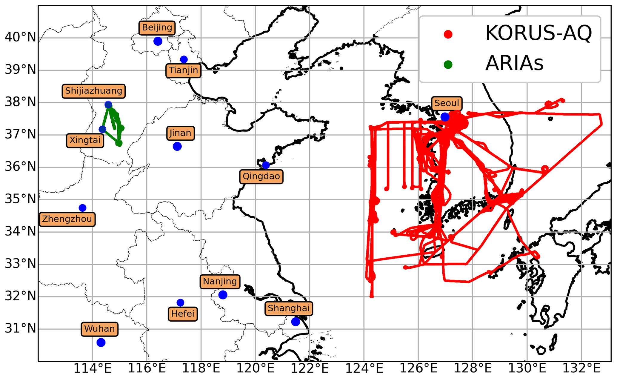
Figure 1 Location of all the KORUS-AQ DC-8 1 min merge measurements (red dots) and of the ARIAs Y-12 1 min merge measurements (green dots). The location of some major cities is also indicated (blue dots).

We evaluate the model output against the DC-8 aircraft measurements, shown in red in Fig. 1, which simultaneously provide many physical and chemical parameters of the tropospheric chemistry environment system (Appendix A). We use the 1 min merge file of DC-8 in situ observations. Model outputs were linearly interpolated to the exact location of the DC-8 in latitude, longitude, pressure altitude, and time from the 6-hourly model outputs. During the whole campaign, Simpson et al. (2020) showed that high benzene concentrations (> 1 ppbv) were only found close to the Daesan petrochemical complex. Since those large gradients of local plumes simply cannot be modeled in a global model, we systematically rejected observations when the benzene proton-transfer-reaction time-of-flight mass spectrometer (PTR-ToF-MS) measurements were higher than 1 ppb.

In order to evaluate the CO sink and the impact of the assimilation of MOPITT CO retrievals on the HO_x levels, we used the OH and HO₂ calculated with the NASA Langley Research Center (LaRC) 0-D time-dependent photochemical box model (Schroeder et al., 2020). This box model is constrained by measured temperature and pressure, photolysis rates derived from actinic flux observations, and observations of O₃, NO, CO, CH₄, CH₂O, PAN, H₂O₂, water vapor, and non-methane hydrocarbons. The production and loss terms of ozone are calculated for every single 1 Hz DC-8 set of observations. This is the only case when we use the 1 s merge file instead of the 1 min merge dataset file. CAM-Chem outputs are interpolated accordingly. While there are some limitations for the species with longer lifetimes, subject to physical processes that are not represented, the box model has been specifically designed to estimate radical concentrations. The details and sensitivity of the calculation are described in Schroeder et al. (2020).

2.2 The ARIAs campaign

The Air Chemistry Research in Asia (ARIAs) field campaign was conducted in May and June 2016 with the goal of better quantifying and characterizing air quality over the NCP (Benish et al., 2020; Wang et al. 2018). The instrumented Y-12 airplane was operated by the Weather Modification Office of the Hebei Province to measure meteorological parameters, aerosols optical properties, and trace gases. The airplane was based at Luancheng Airport, southeast of Shijiazhuang, the capital of Hebei Province, and flew vertical spirals from ∼ 300 to ∼ 3500 m over the cities of Julu, Quzhou, and Xingtai (Fig. 1). There were 11 research fights between 8 May and 11 June 2016. Wang et al. (2018) identified three different planetary boundary layer (PBL) structures with distinct aerosol vertical structure. The aerosol pollution was mostly located below an altitude of 2 km, but sometimes with a vertically inhomogeneous structure, with higher aerosols at higher altitudes than at the surface but still in the boundary layer. These vertical structures were mostly observed when the pollution originated from the southwest and from the eastern coastal region of the study domain, while cleaner air masses originated from the northwest. CO was measured by cavity ring-down spectroscopy with the Picarro model G2401-m instrument with a 5 s precision of 4 ppbv and an estimated accuracy of ±1 %, and O₃ was measured by UV absorption using a thermal electron model 49C ozone analyzer. O₃ values ranged from 52 to 142 ppbv, partly because flight days were chosen to target meteorological conditions favorable to smog events (Benish et al., 2020). CO concentrations ranged from 91 ppbv to about 2 ppmv (Benish et al., 2020). The pervasive high levels of CO correlated with SO₂ indicate of extensive low-tech coal combustion. We rejected individual CO observations (about 5 % of total CO observations) when SO₂ was greater than 20 ppbv (the 95th percentile of all observations) to remove the extremely polluted plumes.

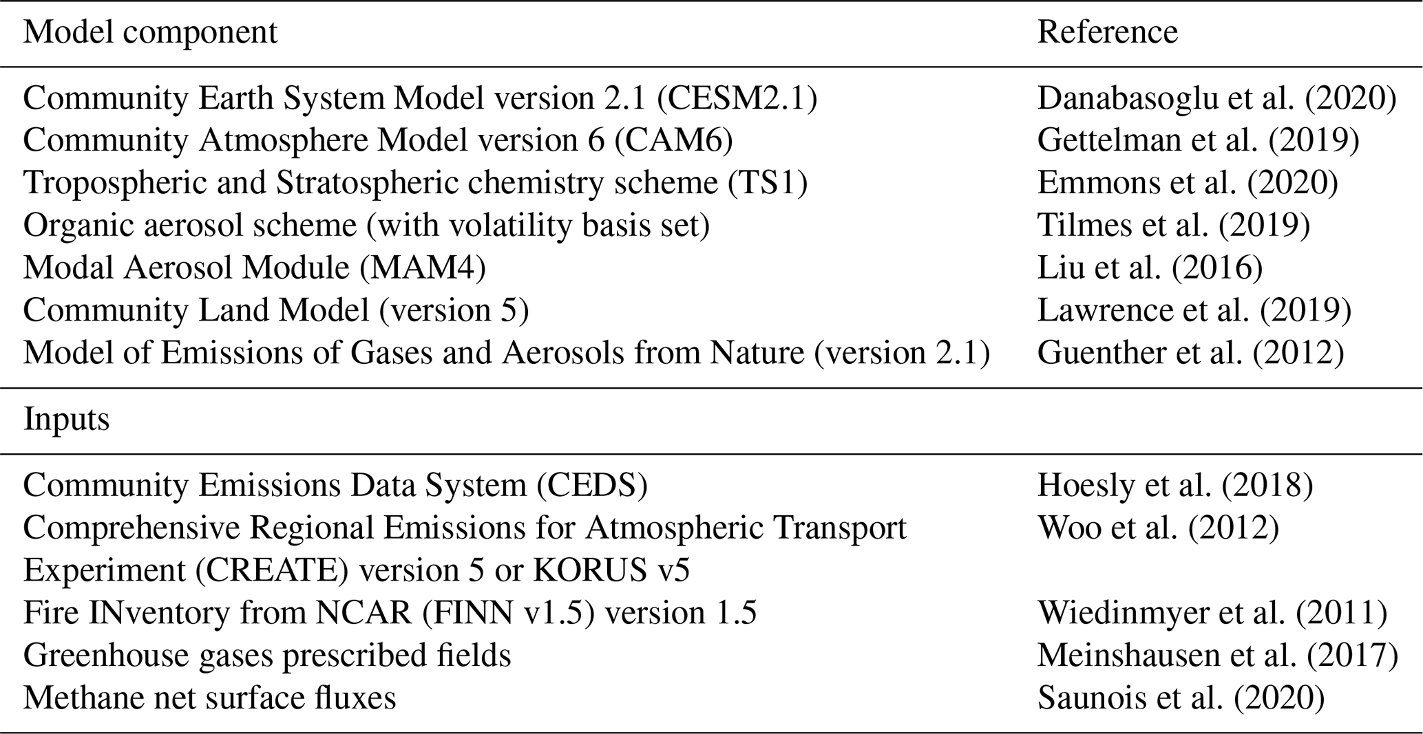
Table 1 Summary of the main model components and references for CESM2.1 and CAM6-Chem.

3 Model configuration and improvements

3.1 Community Atmosphere Model with Chemistry (CAM-Chem)

We use the open-source Community Earth System Model version 2.1 (CESM2.1); an overview of the modeling system and its evaluation is presented in Danabasoglu et al. (2020). It contains many new scientific features and capabilities, including an updated coupler, the Common Infrastructure for Modeling the Earth (CIME), which allows for running an ensemble of CESM runs in parallel with a single executable. The atmosphere is modeled using the finite-volume dynamical core of the Community Atmosphere Model version 6 (CAM6) with 32 vertical levels, a model top at 3.6 hPa, and a 1.25^∘ (in longitude) by 0.95^∘ (in latitude) horizontal resolution (Gettelman et al., 2019). The model now uses a unified parameterization of the planetary boundary layer (PBL) and shallow convection, the Cloud Layers Unified by Binormals (CLUBB; Bogenschutz et al., 2013). Other updates of the model physical parameterizations are described in Gettelman et al. (2019). The new Troposphere and Stratosphere (TS1) reduced gas-phase chemical mechanism contains 221 species and 528 reactions (Emmons et al., 2020) and thus explicitly represents stratospheric and tropospheric ozone and OH chemistry. This chemical scheme contains many updates, including of the isoprene oxidation mechanism, splitting a single aromatic into benzene, toluene, and xylene lumped species as well as a terpene speciation. The overall setup of CESM2.1 has been updated following the protocol of the Coupled Model Intercomparison Project Phase 6, which includes solar forcings (Matthes et al., 2017), surface greenhouse gas boundary conditions (Meinshausen et al., 2017), and anthropogenic emissions. Therefore, we use the anthropogenic emission inventory of chemically reactive gases that has been generated by the Community Emissions Data System (CEDS; Hoesly et al., 2018). We use the latest year available (2014) for the KORUS-AQ period (2016). It is commonly acknowledged that errors in the emission inventory for China are much larger than the trends between different years (Feng et al., 2020). Anthropogenic emissions over East Asia are replaced by the KORUS inventories version 5 or KORUS v5 based on the Comprehensive Regional Emissions for Atmospheric Transport Experiment (CREATE) (Woo et al., 2012). Daily biomass burning emissions are obtained from the Fire INventory from NCAR (FINN v1.5) version 1.5 (Wiedinmyer et al., 2011). Biogenic emissions are modeled within the Community Land Model using the algorithms of the Model of Emissions of Gases and Aerosols from Nature (MEGAN v2.1) (Guenther et al., 2012). A summary of the model references is presented in Table 1. We have made some additional changes for this study, presented in Appendix B. In particular, we updated the heterogeneous uptake of HO₂ and its coefficient.

3.2 Sensitivity test on the biogenic emissions

The KORUS-AQ campaign was subject to photochemical episodes with large concentrations of secondary aerosols and ozone (e.g., H. Kim et al., 2018). There is a significant quantity of biogenic emissions from South Korean forests including deciduous oak trees (Lim et al., 2011) and conifers such as Korean pine (Pinus koraiensis), both of which surround the Taehwa Research Forest. As a result, there are high emissions from a variety of compounds, such as isoprene, monoterpenes, and sesquiterpenes, which contribute to enhanced ozone in favorable conditions (S. Y. Kim et al., 2013; S. Kim et al., 2015, 2016; H.-K. Kim et al., 2018). Oak et al. (2020) showed that the largest ozone production efficiency was in the rural areas of South Korea, where biogenic emissions are dominant. Kim et al. (2014) studied how the plant functional type (PFT) distributions affect the results of biogenic emissions: broadleaf trees, needleleaf trees, shrubs, and herbaceous plants are significant contributors to BVOCs in South Korea. They found large sensitivities of calculated biogenic emissions to three different PFT datasets over Seoul, which resulted in local but significant changes in simulated O₃. We performed a sensitivity analysis to the biogenic emissions by increasing the emission factors for three of the Community Land Model PFTs that are present in Korea: needleleaf evergreen temperate trees, broadleaf evergreen temperate trees, and broadleaf deciduous temperate trees. We perform a set of simulations by varying biogenic emissions to determine the best fit to the observations of formaldehyde (CH₂O) at the surface (see the Supplement). For the sake of clarity, we will present one experiment denoted as CAM_MOP-Bio (see Sect. 4.6).

4 Chemical data assimilation system

4.1 Data Assimilation Research Testbed (DART) implementation

The Data Assimilation Research Testbed (DART) is an open-source community facility for ensemble data assimilation developed and maintained at the National Center for Atmospheric Research (Anderson et al., 2009a). DART has been used in numerous studies for data assimilation (DA) within CESM (Hurrell et al., 2013; Danabasoglu et al., 2020). Global DA analyses have been carried out with assimilation of conventional meteorological datasets within the Community Atmosphere Model (CA; Raeder et al., 2012), the Community Land Model version 4.5 or CLM4.5 (Fox et al., 2018), in a weakly coupled atmospheric assimilation in CAM, and oceanic assimilation in the Parallel Ocean Program ocean model (Karspeck et al., 2018). The chemical data assimilation system inherits from previous work that coupled the ensemble adjustment Kalman filter (EAKF) analysis algorithm (Anderson, 2001) with CAM-Chem. The DART/CAM-Chem is designed for efficient ensemble data assimilation of chemical and meteorological observations at the global scale (Arellano et al., 2007; Barré et al., 2015; Gaubert et al., 2016, 2017).

4.2 DART/CAM-Chem analysis and forecast algorithm

The analysis is carried out using a deterministic ensemble square root filter, the ensemble adjustment Kalman filter (EAKF) (Anderson, 2001, 2003). The ensemble of 30 CAM-Chem members is run with a single executable of CESM using the multi-instance capability. At the analysis step, the following model variables are updated when weather observations are assimilated: surface pressure, temperature, wind components, specific humidity, cloud liquid water, and cloud ice. Assimilated observations include radiosondes as well the Aircraft Communication, Addressing, and Reporting System (ACARS), but also remotely sensed data including satellite drift winds and Global Positioning System (GPS) radio occultation. We use a similar setup as previous studies (Barré et al., 2015; Gaubert et al., 2016, 2017) with a spatial localization of 0.1 radians or ∼ 600 km in the horizontal and 200 hPa in the vertical for both chemical and meteorological observations. We now use the spatially and temporally varying adaptive-inflation-enhanced algorithm (El Gharamti, 2018) that generalizes the scheme of Anderson (2009b). Multiplicative covariance inflation is applied to the forecast ensemble before each analysis step.

4.3 MOPITT assimilation

As in previous implementations, both CO retrievals from MOPITT and meteorological observations are simultaneously assimilated within the DART framework. We assimilate profiles of retrieved CO from the MOPITT nadir sounding instrument onboard the NASA Terra satellite. The MOPITT V8J product (Deeter et al., 2019) is a multispectral retrieval using CO absorption in the thermal infrared (TIR, 4.7 µm) and near-infrared (NIR, 2.3 µm) bands (Worden et al., 2010). The objective is to maximize the retrieval sensitivity to the lower layers of the atmosphere while minimizing the bias. We apply the same filtering thresholds that are used to create the L3 TIR-NIR product, which exclude all observations from Pixel 3 in addition to observations wherein (1) the 5A signal-to-noise ratio (SNR) is lower than 1000 and (2) the 6A SNR is lower than 400. We apply the strictest retrieval anomaly flags (all from 1 to 5). We only assimilate daytime measurements for which latitudes are lower than 80^∘ and when the total column degrees of freedom are higher than 0.5. Super-observations are produced by applying an error-weighted average of the profiles (Barré et al., 2015) on the CAM-Chem grid, with no error correlation since we consider those to be minimized by the strict use of the quality flags, as in Gaubert et al. (2016). In general, MOPITT data have errors smaller than 10 % (Tang et al., 2020; Hedelius et al., 2019), which is much lower than model errors. We evaluate our assimilation results with fully independent aircraft observations.

4.4 Ensemble design

The ensemble of prior emissions is generated by applying a spatially and temporally correlated noise to the given prior emission field, as in previous studies (Coman et al., 2012; Gaubert et al., 2014, 2016, 2017; Barré et al., 2015, 2016). Emission perturbations are generated from a two-dimensional Gaussian distribution with zero mean and unitary variance (Evensen, 2003), with a fixed spatial correlation length. Here we applied the same set of perturbations for every time step, and thus the prior ensemble has a temporal correlation of 1. A different noise distribution is drawn for biomass burning (BB) CO emissions than for anthropogenic direct CO emissions, with a decorrelation length of 250 km for BB and 500 km for direct anthropogenic CO. Thus, as opposed to previous studies, anthropogenic and BB CO sources are completely uncorrelated in the prior ensemble. The same noise is then applied to all the species emitted by the same source, BB or anthropogenic, including NMVOCs, the non-organic nitrogen species, SO₂, and aerosols. This means the added noise in emissions of NMVOCs and CO from the BB or anthropogenic sectors will be completely correlated. We generated another noise sample with a decorrelation length of 500 km for soil emissions of NO.

The ensemble spread in the model physics variables is important for CO, which is directly sensitive to errors in horizontal and vertical winds (both boundary layer height and convection), as well as surface exchange, and indirectly through the impact of dynamics and physics on other chemicals. In particular, a spread in the MEGAN estimates of direct and indirect CO emissions from biogenic sources will be generated from the different atmospheric states passed to the land model. We assigned a spatially and temporally uniform noise drawn from a normal distribution with a standard deviation of 0.1 to the CH₄ emissions. More work will be done to generate a realistic spread in CH₄ emissions, but that is beyond the scope of this study. The ensemble spin-up starts on 1 April 2016 with perturbed emissions described above and with a spread in nudging parameters to perturb the dynamics. After a week, on 7 April 2016, the control run ensemble is initialized from the spin-up; this simulation is not nudged and this period is used to spin up the inflation parameters for the assimilation of the weather observations only. The MOPITT-DA run is initialized from the control run ensemble on 15 April 2016.

4.5 Variable localization and parameter estimation

The multivariate error background error covariance allows for an estimation of the error correlation between the adjusted model variables or state vector and observations. As in previous studies we choose a strict “variable localization” (e.g., Kang et al., 2011) because (1) it is easier to quantify the impacts of the assimilation, such as the chemical response (Gaubert et al., 2016), as well as the model and observations errors (Gaubert et al., 2014), and (2) spurious correlation can have a strong impact on the non-assimilated species that have no constraints. This strict variable localization means that the assimilation of MOPITT only corrects the chemical state vector (i.e., CO), has no impact on the meteorological state vector (U, V, T, Q, P_s), and vice versa. However, we made an exception and extended our chemical state vector by including CO emissions from BB and anthropogenic sources separately and several NMVOCs. We added C₂H₂, C₂H₄, C₂H₆, C₃H₈, benzene, toluene, and the xylene, BIGENE, and BIGALK surrogate species to the state vector. The NMVOCs with a strong anthropogenic and/or BB origin that have a primary sink with OH should be strongly correlated with CO (Miyazaki et al., 2012). The relationships between NMVOCs and CO leads to a correlation in their errors so that the correlation existing in the ensemble will reflect those true errors. In addition to the initial spread described above, spatially and temporally varying adaptive inflation is also applied to the optimized CO surface flux (SFCO) model variable during the analysis procedure.

In CAM-Chem, a diurnal profile is not applied to the emissions; instead, emissions are interpolated from the dates provided in the inventories, which is daily for BB and monthly for anthropogenic sources. The relative increments obtained from the analysis in the form of the surface flux model variable (SFCO) is propagated back to the input file emissions (E) following:

$$\begin{array}{}\text{(2)}& E_i^{\text{analysis}}=E_i^{\text{prior}}\left(\mathrm{1}+w{\displaystyle \frac{\mathrm{\Delta }{\text{SFCO}}_i}{{\text{SFCO}}_i}}\right),\end{array}$$

where i is an ensemble member and $w=a{e}^{-\frac{t}{\mathit{\tau }}}$ is a weight to represent the temporal representativeness and to limit the impact of spurious correlation. At the analysis time (t=0), the weight will be w=a, with a=0.8, i.e., 80 % of the initial increments in Eq. (2). For the other time steps t, the exponential decay characteristic time, τ, is set to 4 d in the case of BB and 4 months in the case of anthropogenic emissions. The impact of the increments will therefore decrease exponentially for the other time steps t from 0.8 to 0, which is imposed (bounded) for 2τ (8 months or 8 d). This makes a strong correction for the current time and the closest time step. This allows for smoothing the increments over time while hopefully leading to a convergence through the sequential correction of the emissions during the assimilation run.

4.6 Simulation overview

In Sect. 5, two simulations with the assimilation of meteorological observations will be presented: the control run and the MOPITT-DA. The difference between the two simulations is the assimilation of MOPITT in the MOPITT-DA run. In the MOPITT-DA assimilation run, the initial conditions of CO and some NMVOCs, as well as CO emission inventories from anthropogenic and biomass burning sources, are optimized during the analysis step. The summary of the simulations presented in the following sections is also presented in Table 2.

In Sect. 6, we compare our emission estimates with a state-of-the-art chemical data assimilation and inversion system, the Tropospheric Chemistry Reanalysis version 2 or TCR-2 (Miyazaki et al., 2019b, 2020b). Miyazaki et al. (2020b) assimilate a variety of satellite instruments using the local ensemble transform Kalman filter (LETKF; Hunt et al., 2007) with the MIROC-Chem model (Watanabe et al., 2011). The setup is fully described and evaluated in Miyazaki et al. (2020b). We regridded the anthropogenic prior and posterior CO estimate from their ${\mathrm{1.125}}^{\circ }\times {\mathrm{1.125}}^{\circ }$ mesh grid to the CAM-Chem grid. In the TCR-2, the prior anthropogenic emission is HTAP v2 for 2010 (Janssens-Maenhout et al., 2015).

Additional sensitivity tests will be performed using deterministic CAM-Chem simulations (Table 2) and presented in Sect. 7. In this case, since no meteorological data assimilation is performed, the dynamics from the prognostic variables U, V, and T need to be nudged towards the NASA GMAO GEOS5.12 meteorological analysis in order to reproduce the meteorological variability. The GEOS analysis is first regridded on the CAM-Chem horizontal and vertical mesh. The nudging is driven by two factors: the strength, a normalized coefficient that ranges between 0 and 1; and the frequency of the nudging, here configured to use 6-hourly outputs from either the GEOS5 reanalysis or our own DART CAM-Chem control run. Based on an ensemble of sensitivity tests (Supplement), we use the nudging setup that minimizes the meteorological errors for the KORUS-AQ observations. This best simulation is the g-post-0.72, hereafter denoted as CAM_Kv5 (Table 2), which will serve as a reference for the additional sensitivity simulation experiments. Aside from the control run and the MOPITT-DA, the CAM-Chem simulations have the same nudging setup and only differ by the CO anthropogenic emissions flux. In addition, the CAM_MOP-Bio is the same as the CAM_MOP but with an overall increase in the MEGAN emission factor. Note that the simulations denoted as CAM_HTAP (TCR-2 prior) and CAM_TCR-2 (TCR-2 posterior) are CAM-Chem simulations with the respective anthropogenic CO emissions from TCR-2. We also use the Copernicus Atmosphere Monitoring Service (CAMS) global bottom-up emission inventory (Granier et al., 2019; Elguindi et al., 2020). We use the CAMS-GLOB-ANTv3.1, which has only minor changes with regards to the most recent version (v4.2). The gridded inventory is available at a spatial resolution of ${\mathrm{0.1}}^{\circ }\times {\mathrm{0.1}}^{\circ }$ and at a monthly temporal resolution for the years 2000–2020. It is built on the EDGARv4.3.2 annual emissions (Crippa et al., 2018) and extrapolated to the most current years using linear trends fit to the years 2011–2014 from the CEDS global inventory. We included artificial CO tracers or “CO tags”, to track the anthropogenic contribution from different geographic area sources (e.g., Gaubert et al., 2016; Butler et al., 2018).

Table 2 Summary of the simulations. The nudging (GEOS) refers to a CAM-Chem deterministic runs with specified dynamics using a nudging to GEOS-FP analysis winds and temperatures (see the Supplement). Aside from the DART simulations (first two rows), all the simulations have the same initial conditions and the same nudging and only change by their anthropogenic CO emissions inputs.

5 Assimilation results: evaluation of the posterior CO during KORUS-AQ

We use the fully independent DC-8 Differential Absorption CO Measurement (DACOM CO) to evaluate the MOPITT assimilation. Figure 2 compares the averaged vertical profiles for the four different mission weather regime phases (Peterson et al., 2019) and the average and standard deviation of all the flights. Observed background CO in the upper free troposphere is between 100 and 125 ppbv and shows a variation of around 10 % between the different phases. The control run shows an average background between 70 and 100 ppbv for the four phases and 80 ppbv for the full KORUS-AQ period, while the MOPITT-DA varies between 80 and 110 ppbv for the four phases with an average of 90 ppbv for the KORUS-AQ period. The root mean square error (RMSE) in MOPITT-DA is reduced by around 10 ppbv compared to the control run for the free troposphere (700 to 300 hPa; Fig. 2).

For the layers closer to the surface, the temporal variations are much stronger. During phase 3, observed CO is 44 % and 30 % higher than the campaign average at 850 and 950 hPa, respectively. While this feature is much better reproduced after assimilation, absolute RMSE values remain large. Overall, the bias is greatly reduced for the MOPITT-DA in the layers between 850 and 650 hPa. We note that the mean CO is still lower than the average observations. The MOPITT-DA shows at the 950 and 850 hPa levels an underestimation of around 30 ppbv, i.e., between 10 % and 20 % lower than the observations. This is in the range of the expected performance given the retrieval uncertainties (10 %) and the spatial footprints of MOPITT pixels (22 km × 22 km)

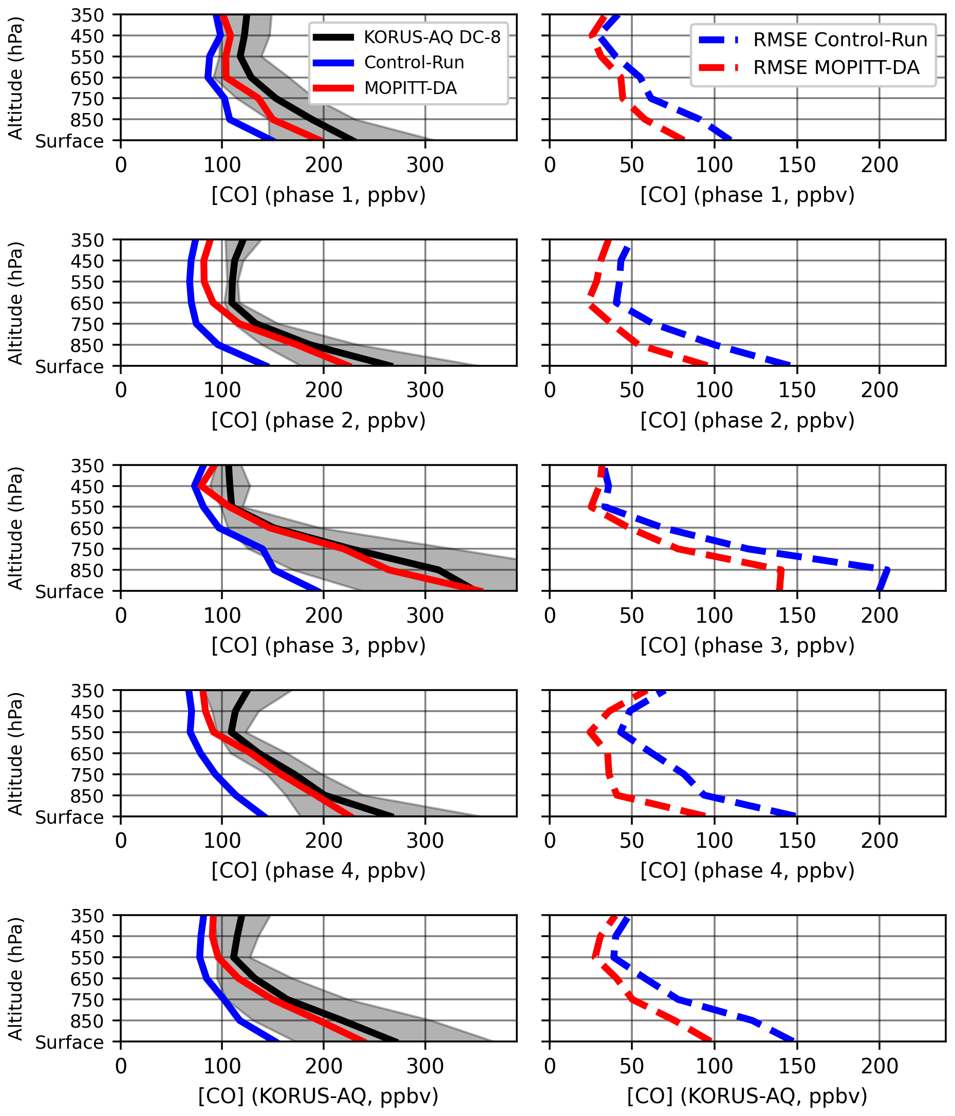
Figure 2 Average CO profiles (left panels) and related RMSE (right panels) for the control run and the MOPITT-DA. The mean (black line) and standard deviation (shaded grey) of the DC-8 observations are calculated for each 100 hPa bin. The first four rows are averaged over the different weather regimes of the campaign (Peterson et al., 2019). The last row displays the average over the whole campaign.

5.1 VOCs state vector augmentation

Concentrations of some VOCs have been added to the state vector and are therefore optimized according to the covariance estimated by the ensemble when MOPITT observations are assimilated. This setup will only provide meaningful corrections if CO and VOC errors are highly correlated through common atmospheric and emission processes and if the ensemble samples those errors in the background error covariance. In this case VOC analysis errors should be reduced by assimilating MOPITT CO, even though VOCs are not directly observed.

Table 3 VOCs added to the state vector, corresponding measuring instrument, and lifetime (Simpson et al., 2020) used for validation. For comparison with surrogate species, the sum of all the corresponding VOC observations is used. WAS stands for whole-air sampler.

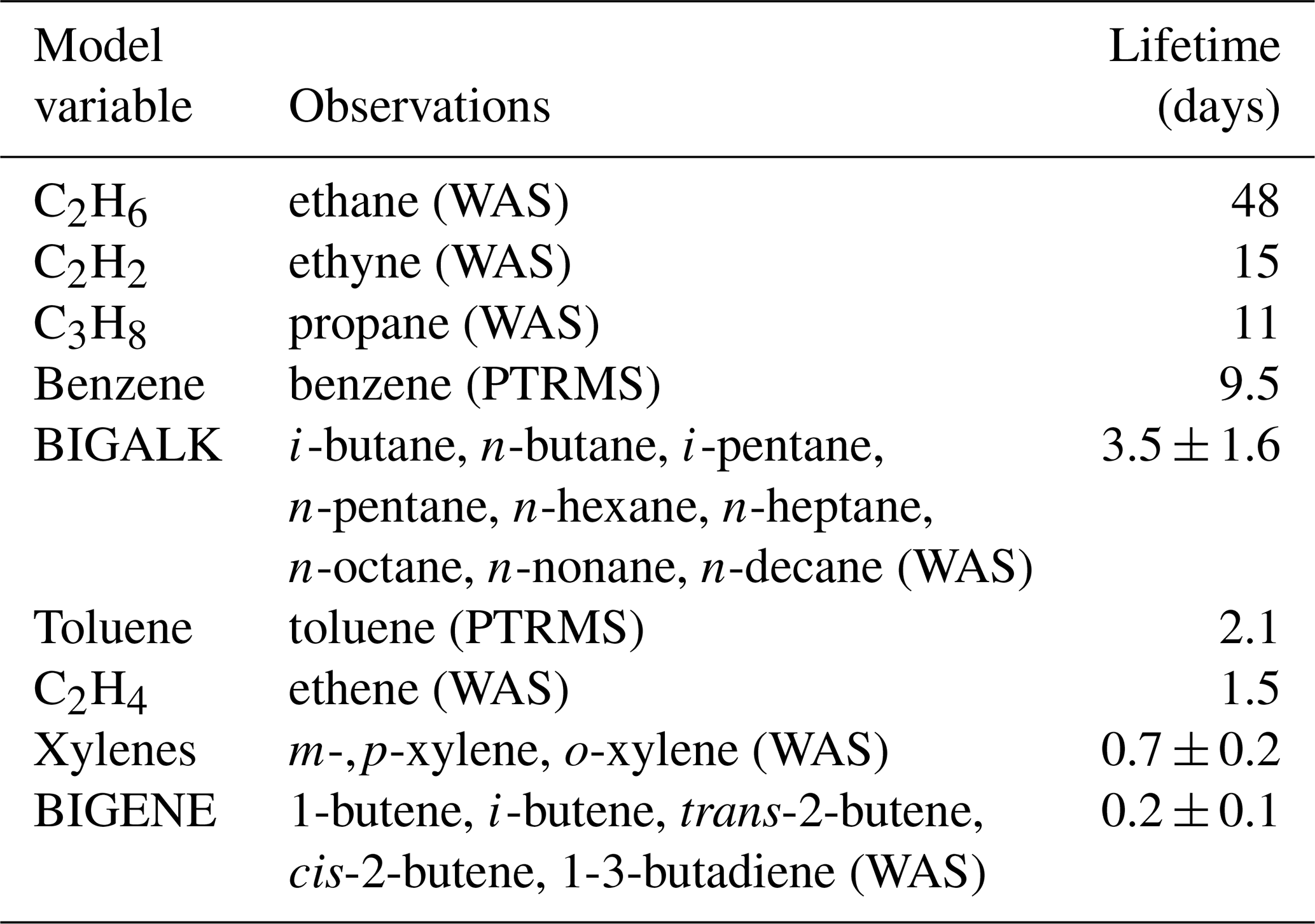
The list of optimized VOCs is shown in Table 3, together with their lifetime and the corresponding species from the whole-air sampler (WAS) instrument used for evaluation. An increase in concentration is found for all nine VOCs in the MOPITT-DA simulation, either because of the state augmentation, and/or because of the reduction in OH due to CO adjustments. Even if the changes are small, this can lead to an increase in errors for the vertical profiles compared to observations when the species is already overestimated in the lower layer of the atmosphere. This is the case for C₂H₄ and BIGENE, the only two species that have substantial biogenic and fire sources, as well as for xylenes and toluene. For all the other species, which are underestimated and are mostly from anthropogenic sources, the assimilation leads to an improvement compared to the observations, mostly by reducing their biases. The best results are obtained for ethane and to a lesser extent propane (Fig. 3). Despite the broad anthropogenic source, ethane and propane originate from sectors that are quite different from CO. However, CO, ethane, and propane have one thing in common, which is that their only atmospheric chemical sink is through OH oxidation. This suggests that a bias in OH leads to correlated errors between CO and alkanes that can be mitigated by including these species in the state vector.

We define a metric of improvement based on the relative change in RMSE that is positive when the RMSE is reduced. Figure 3 shows a clear dependence of this metric on the atmospheric lifetime of the VOCs. All the modeled VOCs with a lifetime shorter than 5 d show an increase in errors, while all the VOCs with a lifetime greater than 10 d are improved, with the largest improvement for ethane, which has a lifetime of 48 d. The relatively large spatial and temporal scales of CO that arise due to its medium atmospheric lifetime significantly limit the ability of CO assimilation to resolve the high-frequency changes in those compounds with short lifetimes. More importantly, this is also to be expected given the limited sensitivity of the MOPITT observations to boundary layer CO.

While satellite observation spatiotemporal resolution and sampling might be improved in the future, NMVOCs with a lifetime shorter than several days should not be included in the state vector when assimilating CO. However, the concentrations of NMVOCs with strong anthropogenic or BB sources and similar chemical characteristics to CO might be significantly improved by the assimilation. We believe that this could also be true for methane.

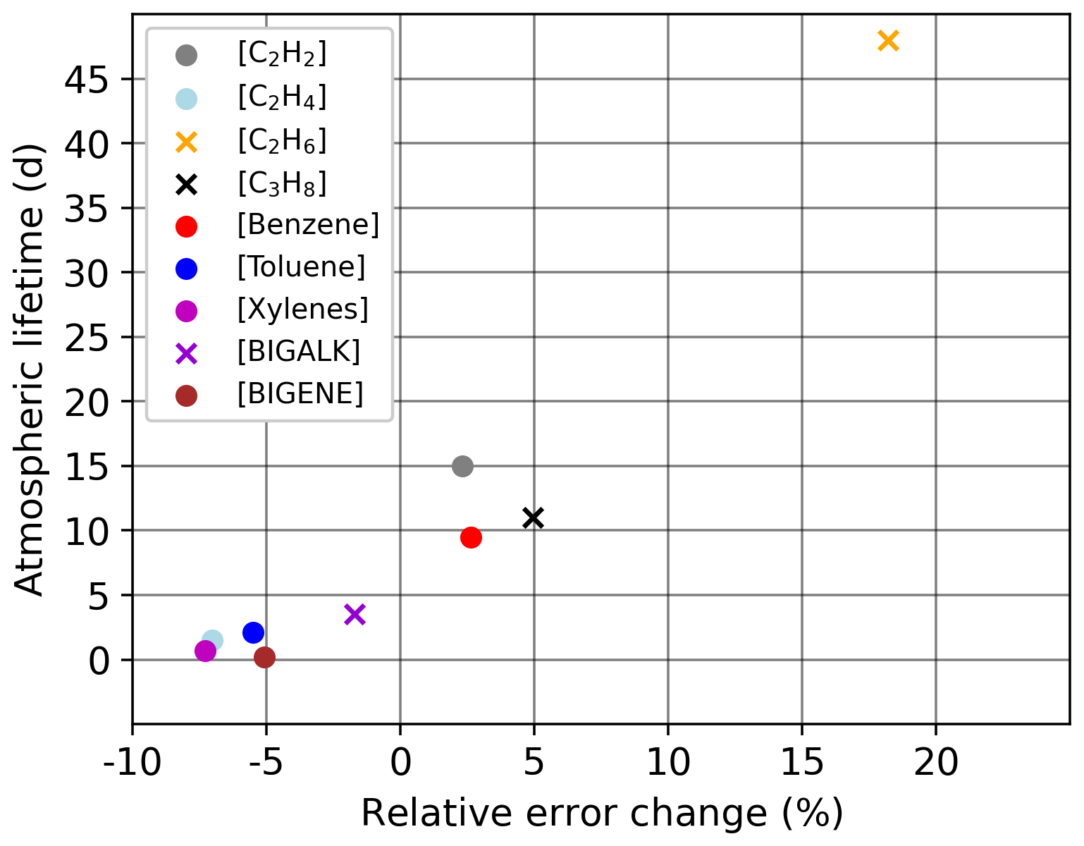
Figure 3 Atmospheric lifetime (from Simpson et al., 2020) in days for the VOCs added to the state vector. Xylenes, BIGALK, and BIGENES are surrogate species, so an average of the lifetimes is calculated. The relative error change is the opposite of the difference in root mean square error relative to the control run (i.e., (control-run-MOPITT-DA) ∕ control run). Thus, a positive relative error change means an improvement compared to the control run.

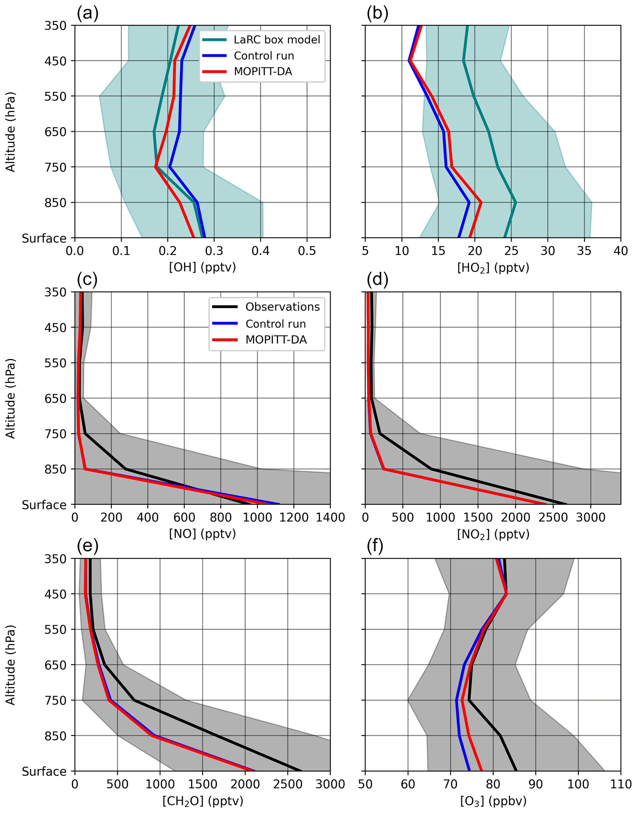
Figure 4 Average vertical profiles of OH (a) and HO₂ (b) for the 1 s merge and the LaRC box model estimates (Schroeder et al., 2020). Results are shown for DC-8 1 min merge observations for NO (c), NO₂ (d), CH₂O (e), and O₃ measurements (f). The shaded area corresponds to the standard deviation around the observed mean.

5.2 Chemical response from MOPITT-DA

This section presents a short summary of the impact of the CO assimilation on the chemical state of the atmosphere and the comparison with unobserved species. Figure 4 shows the average vertical profiles for OH, HO₂, NO, NO₂, CH₂O, and O₃. We use simulated OH and HO₂ from the observationally constrained NASA LaRC box model (Schroeder et al., 2020). The control run and the LaRC box models agree on the mean OH spanning the first two binned layers at lower altitudes. Aloft, the control run overestimates the LaRC box model simulations. The control run underestimates HO₂, which suggests that the excellent agreement on OH in the boundary layer is likely caused by compensating errors. That is, the increase in CO through the MOPITT assimilation decreases the OH concentrations (Gaubert et al., 2016). Here, we find better agreement of the model OH with the observationally constrained LaRC box model simulation at 750 hPa and above. This in turn increases HO₂ and shows a better match with the LaRC box model. This suggests that a small part of the HO₂ underestimation can be explained by the CO underestimation. NO and NO₂ are reasonably well modeled for the surface layer but are underestimated above, with a large underestimation at 850 hPa. An additional comparison with HNO₃, J(O₃), J(NO₂), H₂O₂, and PAN is shown in Fig. S2. The underestimation of NO_x at 850 hPa could be due to the underestimation of NO_x and PAN from upwind source regions. Despite the update of the HO₂ heterogeneous uptake reaction and coefficient presented in Appendix B, the CO increase leads to higher levels of H₂O₂, and the bias is therefore higher in the MOPITT-DA than the control run (Fig. S2). A lower value of the HO₂ heterogeneous uptake coefficient than the one used here (γ=0.1) might produce better results by reducing the HO₂ sink (see Appendix B). It suggests that errors in NO_x and related chemistry drive the underestimation of HO₂ and of the sum of OH and HO₂ (HO_x). Overall, HO_x is underestimated, and OH is fairly well simulated. This suggests that the CO chemical sink alone cannot explain the CO underestimation during the campaign. Alternatively, CH₂O is underestimated in both simulations, suggesting an underprediction of the chemical production of secondary CO. A similar effect to that described in Gaubert et al. (2016) is shown, whereby an increase in CO through the sequential assimilation leads to reduced OH and slows down the VOC oxidation rate and formaldehyde formation, although this is a small effect. In the lower part of the atmosphere, the oxidation of additional CO leads to more effective ozone production and no changes above, consistent with observations. While the errors in NO_x are important, the low CH₂O points to a missing source, which could be due to an underestimation of NMVOCs.

6 Comparison of anthropogenic emission estimates

We show in Fig. 5 the emissions of the prior (CEDS-KORUSv5) and its posterior estimated through the DART/CAM-Chem inversion. It also shows the prior (HTAP v2) from the TCR-2 and its posterior estimate, for which CO emissions are also constrained by MOPITT. We also show the CAMS emissions.

Figure 5 Emissions flux for May 2016 in megagrams of CO per month. Prior (a, CEDS-KORUS v5), TCR-2 prior (b, HTAP v2), and the difference between the two priors (c, TCR-2 prior – prior). Panels (d–f) show the posterior (d, estimated by DART/CAM-Chem), the TCR-2 (e), and the difference between the two posteriors. Panels (g–i) show the emissions increments, the difference between the posterior and the prior (g), and the difference between the TCR-2 and TCR-2 prior (h). The CAMS emissions are shown in panel (i).

Compared to the prior (Fig. 5a), our posterior estimate (Fig. 5d) shows a reduction around the Guizhou Province in southwest China. Larger changes are observed for the Shandong and Henan provinces in central China and over the Yangtze River Delta (Fig. 5g). Increases in emissions are also large in the NCP and the Liaoning Province. While both inversions show a large increase over northern China (Fig. 5g, h), the spatial patterns of the emissions are different between the posterior and the TCR-2 for northern China. The TCR-2 emission increments are located more in the NCP and North Korea (Fig. 5f). Large differences can be identified in central China, in particular over the YRD (Fig. 5h). The Shanghai megacity emissions are higher in the DART/CAM-Chem posterior (Fig. 5d) and the TCR-2 prior (Fig. 5b) than in the TCR-2 posterior (Fig. 5e). A more consistent pattern of larger emissions in the TCR-2 compared to our posterior is found in southern China and the Sichuan Province (Fig. 5f and h). Prior emissions of CO, biogenic and anthropogenic VOCs, and NO_x can all contribute to differences between the TCR-2 and our DART/CAM-Chem estimate. Another important aspect is the 500 km correlation length initial perturbation to generate the ensemble of anthropogenic emissions, combined with a similar localization radius of ∼ 600 km, which explains the large-scale increments found in the DART/CAM-Chem emissions increments (Fig. 5g). The TCR-2 prior show more emissions over North Korea than South Korea (Fig. 5b), and the opposite is true for the DART/CAM-Chem prior (Fig. 6c). This is reflected in the posterior for which the TCR-2 has more emissions in North Korea than the DART/CAM-Chem posterior (Fig. 5f). Compared to its prior, the DART/CAM-Chem posterior emissions are increased by 25 % for South Korea and by 34 % over the SMA. While the CAMS emissions are generally lower (Fig. 5i), the South Korean emissions are higher than in all the other inventories.

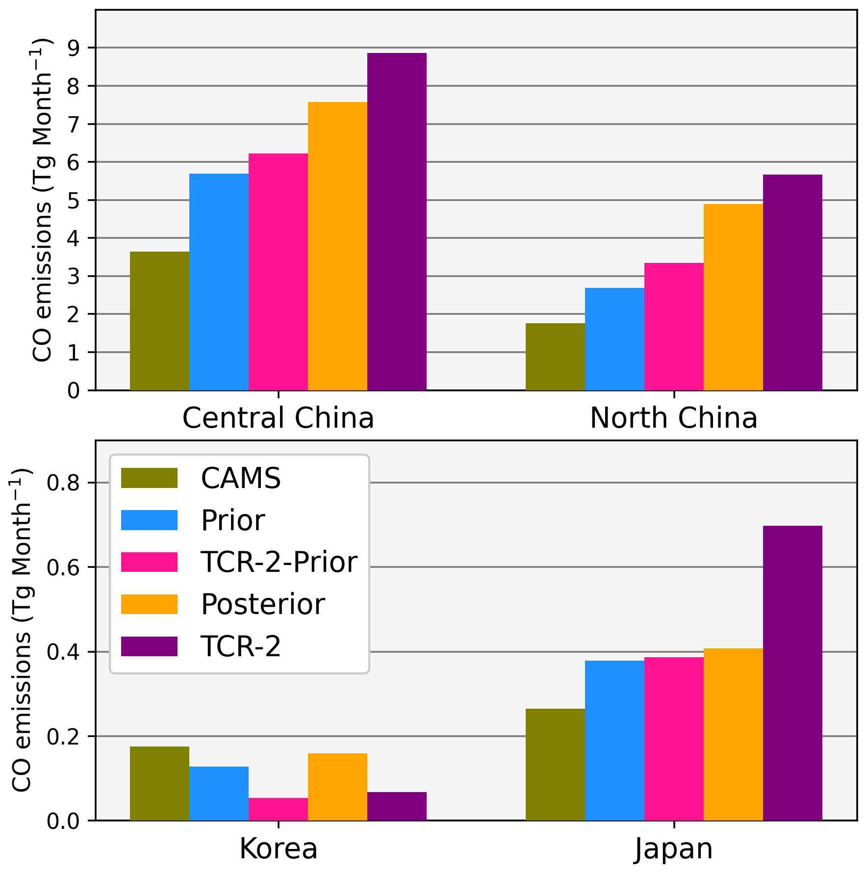
Figure 6 Anthropogenic CO emissions for May 2016 for central China (91^∘ E, 29^∘ N to 124^∘ E, 38^∘ N), North China (91^∘ E, 38^∘ N to 130^∘ E, 49^∘ N), South Korea (125^∘ E, 33.5^∘ N to 129^∘ E, 38^∘ N), and Japan (130^∘ E, 30^∘ N to 146^∘ E, 44^∘ N).

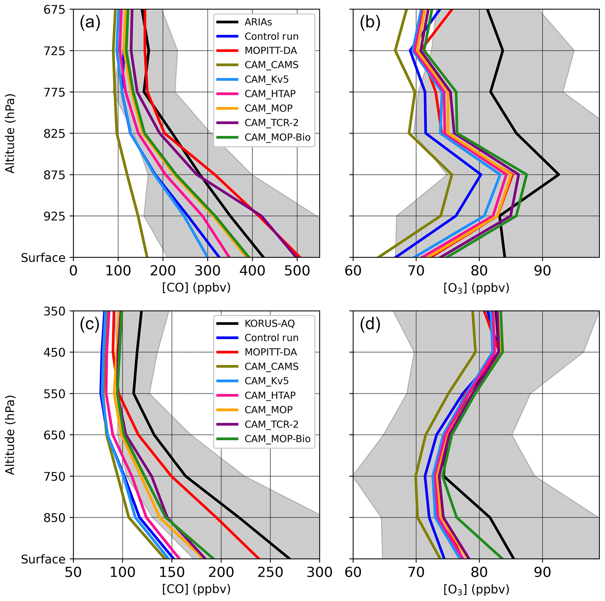
Figure 7 Average CO vertical profiles for the ARIAs campaign (a, b) and KORUS-AQ (c, d). Observations were filtered out when SO₂ was higher than 20 ppbv for ARIAs and benzene higher than 1 ppbv for KORUS-AQ. The black line shows the observation mean, and the shaded area is the observation standard deviation. Only mean CO or O₃ are shown for the model simulations.

Our inversion suggests an underestimation of bottom-up emission inventories for China. The agreement between the posterior emissions for central China is better than for the bottom-up inventory (Fig. 6). The difference between CAMS (3.65 Tg CO per month) and the CEDS-KORUSv5 (5.7 Tg CO per month) is twice as high as the difference between the DART/CAM-Chem posterior (7.6 Tg CO per month) and TCR-2 (8.7 Tg CO per month). On average, the increase in emissions due to assimilation is about 33 % for central China and nearly doubled (80 %) in northern China, from 2.7 to 4.9 Tg CO per month. TCR-2 suggests higher emissions (5.7 Tg CO per month), while the CAMS estimate is lower (1.8 Tg CO per month). More work should be dedicated to check whether the assumptions made on the prior estimates impact the retrieved emissions. This includes improving the regional distribution and scaling up the baseline prior CO emissions, but also how much the model uncertainties in the OH chemical sink impact the CO inversions (e.g., Müller et al., 2018). A comparison of the amount of residential coal-burning emissions in bottom-up inventories could help in understanding the discrepancy and quantifying potential offsets (Chen et al., 2017; M. Cheng et al., 2017; Zhi et al., 2017; Benish et al., 2020).

For South Korea, a relatively smaller difference between the posterior and the prior suggests an improved bottom-up inventory. However, the smaller area of South Korea is much less constrained by MOPITT, and the overall estimate seems to be determined by the prior distribution. For instance, the TCR-2 shows higher emissions over North Korea and the Pyongyang area, while DART/CAM-Chem and CAMS suggest higher emissions for the SMA. Therefore, the CAMS total emissions that show a similar pattern (0.18 Tg CO per month) are in good agreement with the DART/CAM-Chem (0.16 Tg CO per month), while the TCR-2 has a total of 0.07 Tg CO per month. For Japan, where biomass burning and low-tech coal combustion are rare, the total is nearly unchanged in contrast to the other regions, and emissions are increased from 0.38 to 0.41 Tg CO per month or 8 %.

Table 4 Comparison of CO (ppbv) measured aboard the DC-8 and model simulation for all altitudes. Statistical indicators are calculated for phase 1 (seven flight days, 2952 observations), phase 2 (four flight days, 2029 observations), phase 3 (three flight days, 1243 observations), phase 4 (five flight days, 2448 observations), and the whole campaign (20 flight days, 9099 observations).

7 Evaluation of the simulated vertical profiles against ARIAs and KORUS-AQ

This section presents the evaluation of the simulated profiles of CO, O₃, OH, and HO₂ with the observations from ARIAs and KORUS-AQ.

7.1 Mean profile during ARIAs and KORUS-AQ

Figure 7 shows the average CO vertical profiles for the ARIAs and KORUS-AQ campaigns. For the ARIAs field campaign, we bin the profiles into 50 hPa bins. Overall, CO observations show strong variability, with a large enhancement over a background of around 170 ppbv found at 775 hPa and above. Benish et al. (2020) show that the median of the observed CO values in the lowest 500 m is around 400 ppbv. Using additional enhancement ratios, the measurements indicate low-efficiency fossil fuel combustion that could originate from residential coal-burning and gasoline vehicles as well as crop residue burning such as straw from winter wheat. The MOPITT-DA and TCR-2 overestimate the CO concentrations compared to the measurements for this surface layer, although this overestimate is smaller by 60 % for TCR-2 and by 30 % for MOPITT-DA when a value higher than 20 ppbv SO₂ (the approximate 95th percentile) is used to define plumes for exclusion. The CAM-Chem posterior simulated CO concentrations that just use the smoothed posterior emissions from the MOPITT-DA have a mean value closer to the observations. While the two simulations do not have exactly the same transport, the remaining underestimation is likely to be due to the sequential data assimilation in the MOPITT-DA runs that compensates for the remaining biases. Interestingly, the HTAP v2 inventory that was for the year 2010 still provides good CO profiles (CAM_HTAP). The CAM_Kv5, a nudged CAM-Chem simulation, and the control run underestimate the CO concentration, with slight differences due to transport. The modeled profile with CAMS emissions profiles is the lowest CO of all simulations. For altitudes ranging between 900 and 600 hPa, the bias is lowest using the TCR-2 emissions or with the MOPITT-DA because these emissions are more spatially representative of regional pollution (Wang et al., 2018). This confirms that the free-tropospheric background is too low in CAM_Kv5 and CAM_CAMS. The MOPITT-DA naturally shows the lowest bias in CO concentrations in the free troposphere. The 875 hPa (900 to 850 hPa) layer mean (and median) observed ozone during ARIAs (Benish et al., 2020) is around 80 to 90 ppbv, and the mean peaks at 90 ppbv. For this layer, higher O₃ was found for simulations with higher CO. While it suggests that reducing CO biases can improve O₃, NO₂ and NMVOCs such as aromatics seem to play an important role in ozone formation in the region (Benish et al., 2020). The mean O₃ concentration is still underestimated by around 10 ppbv in the free troposphere.

Two groups appear when comparing to KORUS-AQ observations. The control run and CAM_Kv5, using CEDS-KORUS v5 with two different model dynamics and CAM_CAMS, simulate lower CO and show a severe low bias of more than 100 ppbv at the surface. The second group includes the CAM-Chem simulations using posterior emission estimates. Those simulations are quite close together, with an average for all altitude layers of CO of 141 and 145 ppbv and with a bias of 31 % and 29 %, respectively (Table 4). This is to be compared with their priors that have an average CO of 116 and 125 ppbv, which implies an underestimation of 43 % and 39 %, respectively. Correcting only the bias in anthropogenic emissions is not as efficient as the joint optimization of anthropogenic emissions and sequential optimization of initial conditions through data assimilation (MOPITT-DA). It suggests that other sources of error such as transport and chemistry can be mitigated by state assimilation. The MOPITT-DA has an average CO of 179 ppbv, resulting in a 12 % underestimation on average (Table 4), which is well within the range in measurement and representativeness errors. Aside from CAM_CAMS, the modeled free-tropospheric O₃ shows no particular bias. The enhancement of observed O₃ closer to the surface is underestimated in all simulations. The optimized emissions lead to an increase of a few parts per billion in O₃, bringing those simulations closer to the observations. In summary, using top-down estimates of CO emissions clearly improves the CO and O₃ vertical profiles against independent observations over China and Korea.

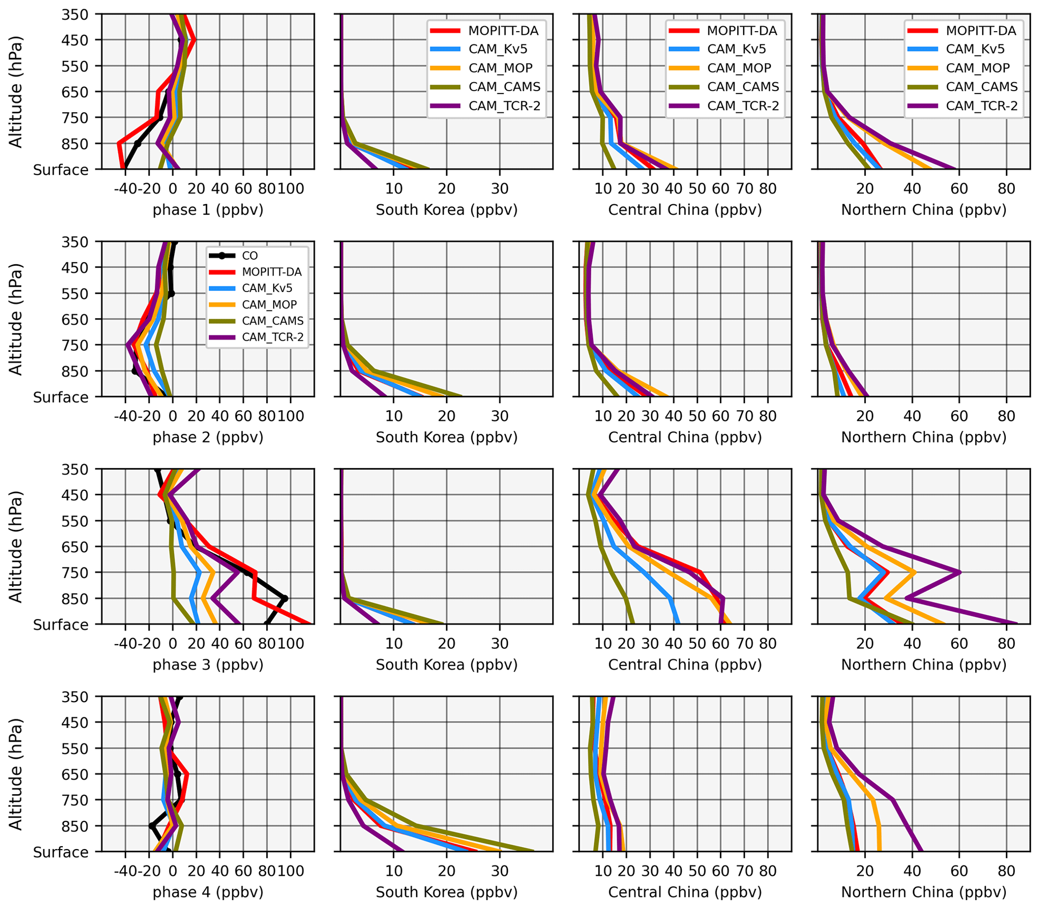
Figure 8 Average CO anomalies for the four different phases of KORUS-AQ (first column). The anomaly is defined by subtracting the respective average vertical profile (see Fig. 2). Absolute vertical profiles of the CO tags are shown from South Korea (second column), central China (third column), and northern China (fourth column). Each row corresponds to a different phase.

7.2 Weather-induced dynamical change in CO during KORUS-AQ

Figure 8 shows the CO anomalies during KORUS-AQ for the observations and the simulations. The CO anomalies are largest in phase 3, with an enhancement of almost 100 ppb at 850 hPa. This transport phase, defined and described in Peterson et al. (2019), was characterized by high levels of ozone (> 60 ppbv) and PM₂₅ (> 50 µg m³) because of efficient transport of low-level pollution (Huang et al., 2018; Miyazaki et al., 2019a; Choi et al., 2019). The model reasonably reproduced the variability of the different phases, albeit with insufficient magnitude. The desired magnitude is only achieved when including data assimilation. Updating the anthropogenic emissions from the bottom-up to the top-down inventories improved the representation of the CO anomalies. This suggests that weather patterns and direct anthropogenic emissions explain some of the CO variability during the campaign. However, since only the MOPITT-DA simulation reproduces the anomalies well, it suggests that chemistry and transport are important too. Large-scale subsidence and reduced wind speeds during the anticyclone of phase 2 were marked by the lowest CO anomalies and are also better reproduced with the updated emissions. Over South Korea, running CAM-Chem with the CAMS emissions shows the highest anthropogenic CO from South Korean sources at the surface for the four phases and is likely to produce more realistic simulations since CO is constantly underestimated. This cannot be seen for the total CO since most of the CO is not from South Korean direct anthropogenic sources. The profile tags of the contributions from central China and northern China are approximately doubled with the optimized emissions, consistent with Tang et al. (2019). As shown in the previous section, the CAM_TCR-2 and the DART/CAM-Chem posteriors have the highest emissions from China and therefore the largest contribution of the CO tags from both northern and central China.

We will now focus on two case studies, phase 2 and phase 3, for which the highest ozone was observed at the surface in South Korea during KORUS-AQ (Peterson et al., 2019).

Figure 9 Average LaRC box model OH and HO₂ as well as measured O₃ for phase 2 (a, c, e) and phase 3 (b, d, f) of KORUS-AQ.

Table 5 Comparison of O₃ measured aboard the DC-8 and model simulation for all altitudes. Statistical indicators are calculated for phase 2 (four flight days, 1910 observations), phase 3 (three flight days 1111 observations), and all of KORUS-AQ.

7.3 Phase 2 case study: the anticyclonic phase

A large-scale anticyclone occurred from 17 to 22 May 2016 with increased surface temperatures, reduced wind speed, and drier conditions, all of which enhance ozone production (Peterson et al., 2019). The conditions were also favorable to an increase in biogenic emissions. As shown in the previous sections, this episode was characterized by negative CO anomalies that were best captured by the MOPITT-DA simulations. This anomaly is reflected through lower OH and higher O₃ between 800 and 400 hPa (Fig. 9). This indicates rather clean air masses, probably with a larger stratospheric contribution. This episode is driven by the overall weather pattern with a clear enhancement of HO_x and O₃ towards the surface. In this case, changes in anthropogenic CO only play a minor role, and O₃ is still modeled better with a reduction of the bias by 1 ppbv between the posterior and the prior (Table 5). The increase in biogenic emissions leads to an improvement in O₃ by further reducing the bias at the surface (Fig. 9). Over the whole profile, the bias is reduced by 3 ppbv (4 ppbv against the prior) for the CAM_MOP-Bio compared to the CAM_MOP, with a reduction in RMSE as well (Table 5).

7.4 Phase 3 case study: low-level transport and haze development

Phase 3 was characterized by the largest observed CO and O₃ positive anomalies. In this case, there is a clear relationship between the CO bias and the O₃, OH, and HO₂ vertical profiles (Fig. 9). The OH is overestimated because of a lack of CO, other VOCs, and errors in the vertical profile of NO_x. Increasing CO in the CAM_MOP reduces OH and increases HO₂ and O₃. The overall bias (Table 5) in ozone is reduced from 11.3 ppbv to 9.9 ppbv with the change in CO and lowered further to 7.3 ppbv with the additional increase in biogenic emissions (CAM_MOP-Bio). The relative impacts of biogenics are clear in the surface layer for OH, HO₂, and O₃. Overall, HO₂ and O₃ are underestimated as a result of CO underestimation. The MOPITT assimilation provides the best results for OH throughout the profile as well as a lower RMSE and a similar bias as the CAM_MOP-Bio (Table 5). As suggested by the Chinese origin of the pollution for higher levels, it is likely that additional anthropogenic NMVOCs are also missing and contribute to the ozone formation that is still underestimated.

8 Conclusions

Anthropogenic CO emissions are an important contributor to poor summer air quality in Asia and to forward modeling uncertainties. Here we evaluate top-down estimates of the CO emissions in East Asia with aircraft observations from two extensive field campaigns. There are multiple lines of evidence that the bottom-up anthropogenic emissions are too low in winter and spring, leading to a large underestimation of CO during the KORUS-AQ campaign in May and June 2016. We also highlight in this work the fact that chemical production and loss via OH reaction from emissions of anthropogenic and biogenic VOCs confound the attribution of this bias in current model simulations. Combined initial conditions and emission optimization remains the best method to overcome these modeling issues. The major findings of this investigation are the following.

1. The comparison of OH modeling and observations confirms that assimilating CO improves the OH chemistry by correcting the OH ∕ HO₂ partitioning. The interactive and moderately comprehensive chemistry with resolved weather from reanalysis datasets represents the variations in OH well. These results provide an additional line of evidence that assimilating CO improves the representation of OH in global chemical transport models. This has implications for studying the CH₄–CO–OH coupled reactions and the impact of chemistry and interactive chemistry for allowing feedbacks. It suggests that even if global mean OH is buffered on the global scale, local changes in OH can be important and can be quantified by taking advantage of field campaigns. This will create ways to improve and provide additional constraints on CH₄ inversions by either improving the sink or by better characterizing anthropogenic sources through CO assimilations. A better quantification of the spatiotemporal variability of these compounds will improve the physical representation of Earth system processes and feedbacks and will be beneficial for both air quality and climate change mitigation scenarios.

2. The setup of the CO assimilation that corrects the initial conditions and emissions provides the best results for CO. While the emission update improves the forecast closer to the source, the assimilation allows for better reproduction of the vertical profiles and the background and eventually compensates for model errors.

3. The spread of emission estimates from state-of-the-art inventories, three bottom-up and two top-down, is significant. For example, the emissions in central China show a range from 3.65 to 8.87 Tg CO per month. Inventories with the highest emissions fluxes show improved vertical profiles of CO.

4. Running the forward model with updated emissions of anthropogenic CO increases the O₃ formation, reduces OH, and increases HO₂. This improves the comparison with O₃, OH, and HO₂ observations. The comparison with observations suggests that the overall modeled photochemistry was improved with updated CO emissions. In this case, there is also a better representation of severe pollution episodes with large O₃ values. Often overlooked, it clearly shows that running chemistry transport models with biased CO and VOC emissions results in poorly modeled ozone and impacts most of the chemical state of the atmosphere. The sensitivities may vary for different chemical and physical atmospheric environments. In this case, underestimating CO in VOC-limited chemical regimes explains the underestimation of ozone in the boundary layer and the lower free troposphere.

5. Biogenic emissions appear to play an important role in ozone formation over South Korea, in particular when conditions are favorable (sunny and warm). The role is weaker over China, at least in May before maximum biogenic emission rates. A combined assimilation of CO and CH₂O observations is likely to greatly improve ozone forecasting through estimates of boundary and initial condition estimates of VOCs.

On top of CO data assimilation, improved emissions through state augmentation can help improve the next generation of Korean (e.g., Lee et al., 2020) or global (Barré et al., 2019) air quality analysis and forecasting systems. Further improvements can be achieved by simultaneously assimilating CH₂O retrievals (e.g., Souri et al., 2020) and CO retrievals. Improving the aerosol distribution can help correct the HO₂ uptake and therefore OH, CO, and O₃ by assimilating satellite aerosol optical depth measurements, in particular for this region with high aerosol loadings (e.g., Ha et al., 2020). Using CrIS–TROPOMI joint retrievals (Fu et al., 2016), the improved vertical sensitivity may potentially be used to further constrain secondary CO formed through biogenic oxidation. In this case, secondary CO is correlated with ozone formation. This is also true for other geographical areas, such as over the United States in summer (Y. Cheng et al., 2017, 2018). On average, there is a lower combustion efficiency in China than in Korea, with the ratio of CO to CO₂ changing accordingly as shown by the DC-8 measurements during KORUS-AQ (Halliday et al., 2019) and indicated by model simulations (Tang et al., 2018). Tracking CO₂ and CO from fossil fuel emissions could be combined to further constrain fossil fuel emission fluxes.

Many studies have focused on the long-term CO emission trends now well characterized (Zheng et al., 2019). For the sake of forward modeling (see, e.g., Huang et al., 2018), it is important to focus on improving the absolute emission totals and their spatiotemporal distribution. While bottom-up inventories are critical, the next step is a comparison of inverse modeling estimates in combination with aircraft observations (e.g., Gaubert et al., 2019) to assess transport, chemistry, and deposition error. Multi-model estimates of the emissions will provide improved error bars on the CO budget and hopefully reduced uncertainties from chemistry and meteorology (e.g., Müller et al., 2018; Miyazaki et al., 2020a).

Appendix A: KORUS-AQ DC-8 instrumentation

CO and CH₄ were both measured using the fast-response (1 Hz), high-precision (0.1 % for CH₄, 1 % for CO), and high-accuracy (2 %) NASA Langley Differential Absorption CO Measurement or DACOM (Sachse et al., 1987). Based on the differential absorption technique, CO and CH₄ were measured using an infrared tunable diode laser. The instrument has been used in many field campaigns and has been useful to evaluate profiles retrieved from satellite remote sensing of CO (Warner et al., 2010; Tang et al., 2020). Formaldehyde was measured using the Compact Atmospheric Multispecies Spectrometer (CAMS), also at 1 Hz (Richter et al., 2015). NO, NO₂, and O₃ were measured by the NCAR chemiluminescence instrument (Ridley and Grahek, 1990; Weinheimer et al., 1993). Nitric acid (HNO₃), hydrogen peroxide (H₂O₂), and methyl hydroperoxide (CH₃OOH) were measured using the California Institute of Technology Chemical Ionization Mass Spectrometer (CIT-CIMS) (Crounse et al., 2006). Among the 82 speciated VOCs from discrete whole-air sampling (WAS) followed by multicolumn gas chromatography (Simpson et al., 2020), we used ethyne (C₂H₂), ethane (C₂H₆), ethene (C₂H₄), and propane (C₃H₈). All the larger alkanes (i-butane, n-butane, i-pentane, n-pentane, n-hexane, n-heptane, n-octane, n-nonane, n-decane), alkenes (1-butene, i-butene, trans-3-butene and 1-3-butadiene), and xylenes (m-,p-xylene, o-xylene) were summed (Table 3) for comparison with the BIGALK, BIGENE, and xylenes, respectively, of the T1 surrogate species (Emmons et al., 2020). Methanol (CH₃OH), acetaldehyde (CH₃CHO), acetone (CH₃COCH₃), benzene (C₆H₆), and toluene (C₇H₈) were measured with the proton-transfer-reaction time-of-flight mass spectrometer (PTR-ToF-MS) at 10 Hz frequency (Müller et al., 2014). We also evaluate some meteorological parameters (Chan et al., 1998), such as temperature, wind speed, and water vapor moist volumetric mixing ratio measured by the NASA open-path diode laser hygrometer (Diskin et al., 2002; Podolske et al., 2003), with a 5 % uncertainty. J values were measured using the CAFS instrument (Charged-coupled device Actinic Flux Spectroradiometer; Shetter and Müller, 1999; Petropavlovskikh et al., 2007).

Appendix B: CAM-Chem updates

B1 CH₄ emissions from the Global Carbon Project CH₄

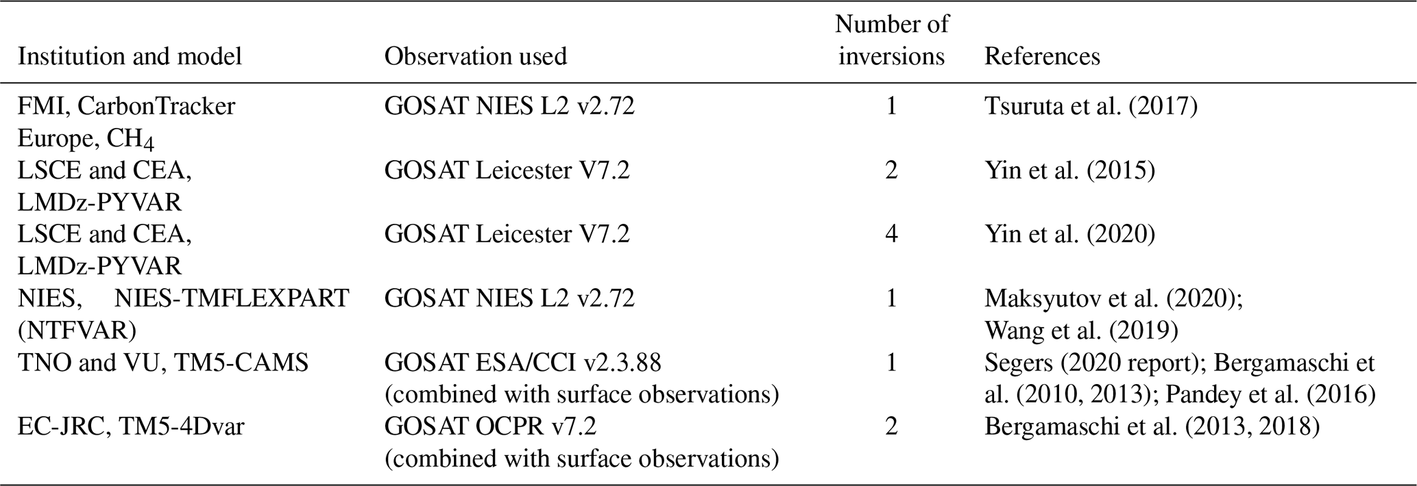
Radiatively active species, such as CH₄, are prescribed in CAM-Chem using a latitudinal monthly surface field derived from observations in the past and projections for the future, defined in the CMIP6 protocol (Meinshausen et al., 2017). In order to include the feedbacks in the CH₄–CO–OH chemical mechanism, we choose to apply CH₄ emissions instead of the prescribed field. The scope of the paper is not to study the methane budget; the objectives are to see how much CO is produced from CH₄ during the campaign. The long-term goal is to get sensitivities to changes according to CO emission updates in order to analyze the feedbacks on CH₄ when CO is changed. We used emissions from some of the inversions of a recent compilation of the CH₄ budget from top-down estimates (Saunois et al., 2020). As a first step, we used the mean of the 11 inversions (Table B1) that assimilate CH₄ retrievals from the JAXA Greenhouse Gases Observing SATellite (GOSAT; Kuze et al., 2009).

Table B1 List of the 11 methane inversions from the global methane budget (Saunois et al., 2020), as indicated by the column showing the number of inversions. All the details are presented in the references.

B2 The HO₂ uptake by aerosol particles

The TS1 chemistry includes an HO₂ uptake by aerosol particles following the recommendation of Jaeglé et al. (2000) and Jacob et al. (2000), which forms H₂O₂ with a reactive uptake coefficient γ of 0.2, as follows:

$$\begin{array}{}\text{(B1)}& {\mathrm{HO}}_{\mathrm{2}}+\text{aerosols}\to \mathrm{0.5}\times {\mathrm{H}}_{\mathrm{2}}{\mathrm{O}}_{\mathrm{2}}\text{with}\mathit{\gamma }=\mathrm{0.2}.\end{array}$$

Based on Observations from the NASA Arctic Research of the Composition of the Troposphere from Aircraft and Satellites (ARCTAS) and other field campaigns, Mao et al. (2010, 2013) suggested a catalytic mechanism with transition metal ions (Cu and Fe) that rapidly converts HO₂ to H₂O instead of H₂O₂:

$$\begin{array}{}\text{(B2)}& {\mathrm{HO}}_{\mathrm{2}}+\text{aerosols}\to {\mathrm{H}}_{\mathrm{2}}\mathrm{O}\text{with}\mathit{\gamma }=\mathrm{0.2}.\end{array}$$

Using Eq. (B2) and γ=1 leads to a large loss of HO_x, which in turn increases the CH₄ and CO lifetime and thus reduces the CO bias during the high-latitude winter (Mao et al., 2013). Christian et al. (2017) simulated a range of possible values of γ, evaluated the results against ARCTAS data, and found that lower γ, closer to zero, gave a more realistic distribution of HO_x. Kanaya et al. (2009) studied ozone formation over Mount Tai, located in central East China, and looked at the possible influence of the heterogeneous loss of gaseous HO₂ radicals. They found that introducing the loss reduces HO₂ levels and increases ozone, with a more pronounced effect in the upper part of the boundary layer where the role of OH + NO₂ + M reaction does not play a significant role in the radical termination reaction, while the number density of aerosol particles is still important. Li et al. (2018) found that the HO₂ uptake was the largest HO_x sink in the upper boundary layer in northern China. They suggested that the reduction in HO₂ uptake caused by the decrease in aerosols was responsible for the increase in O₃ in the region. Thus, the initial comparison of CAM-Chem using Eq. (B1) showed a large overestimation of H₂O₂. In a previous study using Eq. (B1), the increase in CO following data assimilation increased hydrogen peroxide (H₂O₂) levels (Gaubert et al., 2016). Therefore, it is expected that hydrogen peroxide (H₂O₂) would be severely overestimated if Eq. (B1) is used. Miyazaki et al. (2019a) assimilated several satellite retrievals of chemical composition during KORUS-AQ, including MOPITT, and found a strong overestimation of H₂O₂ using Eq. (B1) in the chemical scheme of the MIROC-Chem model. Thus, the reaction in CAM-Chem has been updated to Eq. (B2) with γ=0.1 prior to any data assimilation run.

B3 Results on HO₂ uptake and methane emissions

This section presents the results of the model update before the assimilation runs are conducted. Five CAM-Chem simulations were performed (Table B2), and CAM-Chem-Ref corresponds to the reference with prescribed CH₄ and Eq. (B2) for the HO₂ uptake. CAM-H2O is performed with the update to Eq. (3) for the HO₂ uptake, and GCP-Ref is performed with the CH₄ emissions instead of the CH₄ prescribed field. GCP-H2O contains the update of CH₄ emissions and of the HO₂ uptake and has been run with γ=0.2 and γ=0.1.

Table B2 Description of the sensitivity test performed with CAM-Chem before any assimilation run.

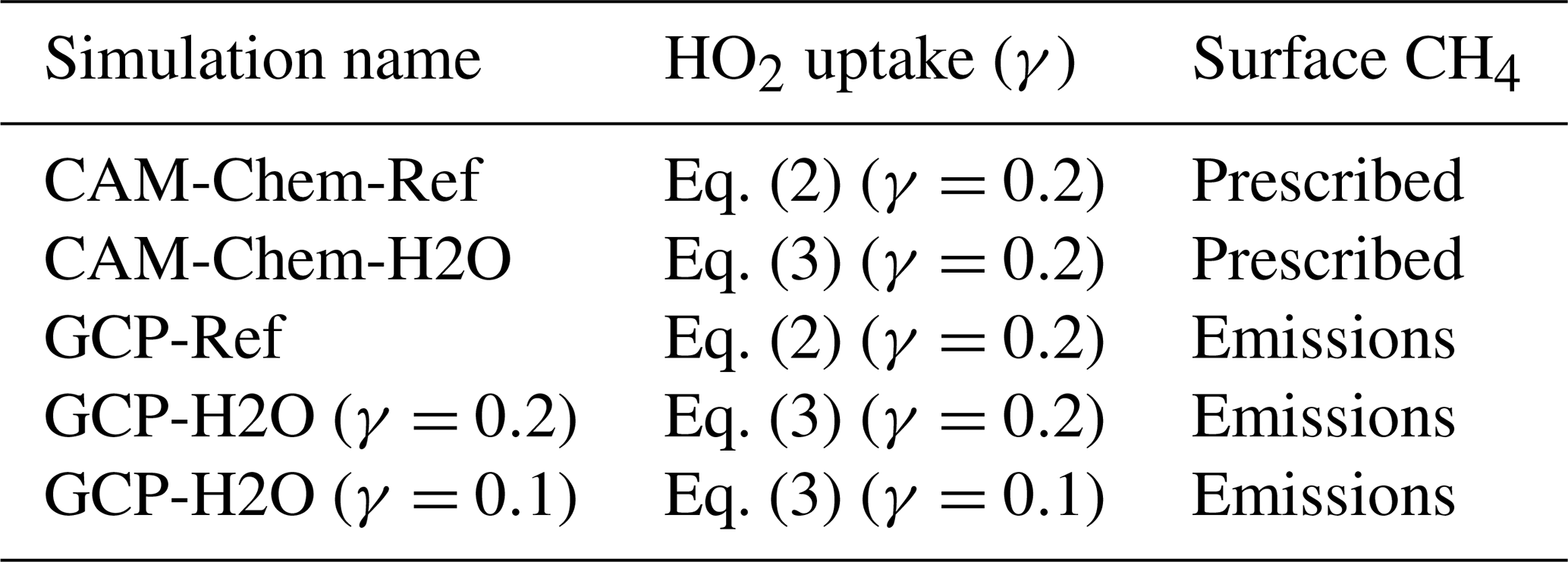
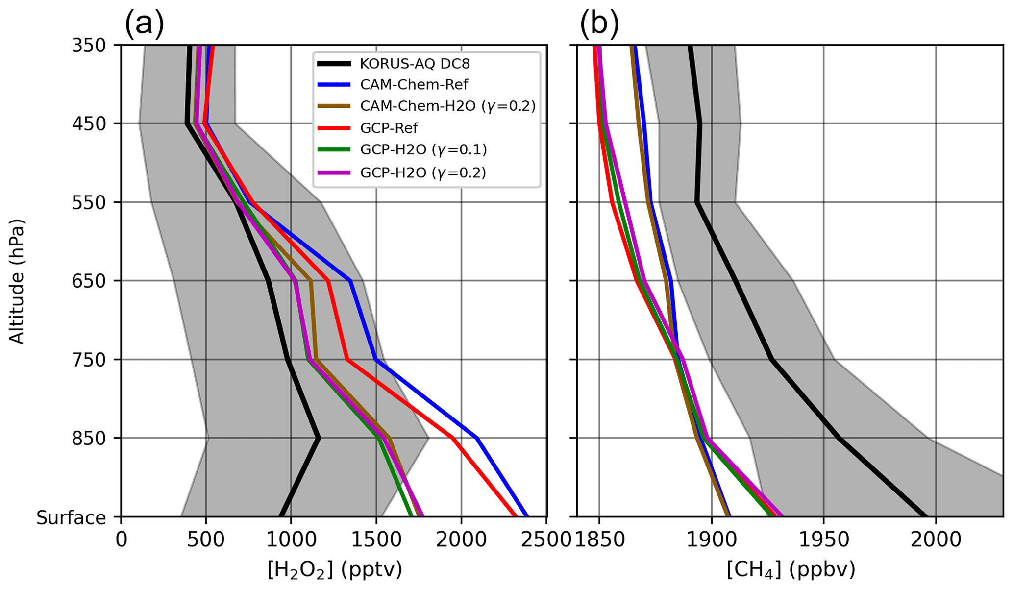
Figure B1 Average H₂O₂ profiles (a) and CH₄ profiles (b) for KORUS-AQ. The mean (black line) and standard deviation (shaded grey) of the DC-8 observations are calculated for each 100 hPa bin, and only the mean is shown for model simulations.

Figure B1 shows the average profiles for H₂O₂ and CH₄. There is a large bias in H₂O₂ for the reference simulation (CAM-Chem-Ref) that is particularly large in the surface layer. The observed H₂O₂ at the surface is lower in the morning due to inhibited photochemical production and nighttime deposition (Schroeder et al., 2020). Large model errors could then be due to uncertainties in the boundary layer height and wet deposition. However, this points to an underestimation of H₂O₂ dry deposition, a common feature found due to an overestimation of surface resistance (Ganzeveld et al., 2006; Nguyen et al., 2015). The H₂O₂ daytime deposition velocities calculated at the location of the Taehwa Research Forest ranged between 0.4 and 1.3 cm s⁻¹, which suggests an underestimation compared to the observed velocities of around 5 cm s⁻¹ reported in the literature (Hall and Claiborn, 1997; Hall et al., 1999; Valverde-Canossa et al., 2005; Nguyen et al., 2015). A simulation with a 5-fold increase in the H₂O₂ deposition velocity over land only partially reduces the H₂O₂ bias. Further work needs to be done to better understand the drivers of the H₂O₂ biases, which is beyond the scope of this study.

Interestingly, having CH₄ emissions (GCP-Ref) while keeping the original reaction (Eq. 2) gives a slightly better H₂O₂, suggesting that using optimized emissions instead of a prescribed concentration field has an effect on the oxidant distribution. The three simulations with the updated chemistry outperform the references with biases almost halved. This is particularly true for the free troposphere. The modeled H₂O₂ profile seems rather insensitive to the choice of the γ value. Since the simulations with γ=0.1 perform slightly better, all following simulations will be done with the updated reaction and γ=0.1. This is consistent with a recently published study that diagnosed a median γ value of 0.1 over the NCP region (Song et al., 2020).

Using emissions instead of fixed boundary conditions improves the simulated CH₄ near the surface, but with a lower tropospheric background (Fig. B1). The comparison with CH₄ observations indicates a general underestimation. At this point, it is difficult to determine why it is underestimated.

A first reason could be a CH₄ sink in the model that is too strong compared to the sink considered in the inversions that derived the GCP emissions. However, the prescribed CH₄ is not resolved in longitude, while the difference for a given latitude can be up to 300 ppb when using emissions (see Fig. S1). Emissions also have uncertainties and could be underestimated, or they may have just been estimated with lower OH than the one CAM-Chem simulates for this period. Saunois et al. (2020) showed that GOSAT-based inversions have lower emissions than surface-based inversions for the northern midlatitudes. It is likely that the errors observed during KORUS-AQ are a combination of both of those factors, as well as potential transport errors. Since the CH₄ profile is overall better reproduced with the GCP emissions, we have used the ensemble mean of the 11 GCP optimized emissions for the simulations presented in the main paper.