Evaluating trends and seasonality in modeled PM_2.5 concentrations using empirical mode decomposition

Regional-scale air quality models are being used for studying the sources, composition, transport, transformation, and deposition of fine particulate matter (PM_2.5). The availability of decadal air quality simulations provides a unique opportunity to explore sophisticated model evaluation techniques rather than relying solely on traditional operational evaluations. In this study, we propose a new approach for process-based model evaluation of speciated PM_2.5 using improved complete ensemble empirical mode decomposition with adaptive noise (improved CEEMDAN) to assess how well version 5.0.2 of the coupled Weather Research and Forecasting model–Community Multiscale Air Quality model (WRF-CMAQ) simulates the time-dependent long-term trend and cyclical variations in daily average PM_2.5 and its species, including sulfate (SO₄), nitrate (NO₃), ammonium (NH₄), chloride (Cl), organic carbon (OC), and elemental carbon (EC). The utility of the proposed approach for model evaluation is demonstrated using PM_2.5 data at three monitoring locations. At these locations, the model is generally more capable of simulating the rate of change in the long-term trend component than its absolute magnitude. Amplitudes of the sub-seasonal and annual cycles of total PM_2.5, SO₄, and OC are well reproduced. However, the time-dependent phase difference in the annual cycles for total PM_2.5, OC, and EC reveals a phase shift of up to half a year, indicating the need for proper temporal allocation of emissions and for updating the treatment of organic aerosols compared to the model version used for this set of simulations. Evaluation of sub-seasonal and interannual variations indicates that CMAQ is more capable of replicating the sub-seasonal cycles than interannual variations in magnitude and phase.

1 Introduction

It is well recognized that inhalable fine particulate matter (PM_2.5) adversely impacts human health and the environment. Regional-scale air quality models are being used in health impact studies and decision-making related to PM_2.5. Long-term model simulations of PM_2.5 concentrations using regional air quality models are essential to identify long-term trends and cyclical variations such as annual cycles in areas larger than what is covered by in situ measurements. However, total PM_2.5 concentrations are challenging to predict because of the dependence on the contributions from individual PM_2.5 components, such as sulfates, nitrates, carbonaceous species, and crustal elements. In this context, a detailed process-based evaluation of the simulated speciated PM_2.5 must be carried out to ensure acceptable replication of observations so model users can have confidence in using regional air quality models for policymaking. Furthermore, process-based information can be useful for making improvements to the model.

Some of the trend or step change evaluations of regional air quality models in the past have focused on specific pairs of years (Kang et al., 2013; Zhou et al., 2013; Foley et al., 2015). These studies do not properly account for the sub-seasonal and interannual variations between those specific periods. Trend evaluation is commonly done by linear regression of indexes such as the annual mean or specific percentiles, assuming linearity and stationarity of time series (Civerolo et al., 2010; Hogrefe et al., 2011; Banzhaf et al., 2015; Astitha et al., 2017). The problem with linear trend evaluation is that there is no guarantee the trend is actually linear during the period of the study because the underlying processes are in fact nonlinear and nonstationary (Wu et al., 2007).

Seasonal variations are usually studied and evaluated by investigating the monthly or seasonal means of total and/or speciated PM_2.5 (Civerolo et al., 2010; Banzhaf et al., 2015; Yahya et al., 2016; Henneman et al., 2017). Evaluation of 10-year averaged monthly mean (i.e., 10-year averaged mean in Jan., …, Dec.) of PM_2.5 simulated with WRF-Chem (Weather Research and Forecasting model coupled with Chemistry) against the Interagency Monitoring of Protected Visual Environments (IMPROVE) by Yahya et al. (2016) shows that the model captures the observed features of summer peaks in PM_2.5 with a phase shift of a few months. However, according to the analysis (Fig. 10) in Henneman et al. (2017), the seasonality shown in monthly averaged PM_2.5 time series is much less distinguishable compared with that of ozone, and the Community Multiscale Air Quality model (CMAQ, version 5.0.2) does not replicate the monthly PM_2.5 very well, with large underestimation in the summer months. In these studies, the seasonality might not be well represented by the preselected averaging window size of 1 or 3 months. In addition, averaging of these monthly or seasonal means across multiple years may conceal the long-term trends or interannual variations driven by climate change, emission control policies, or other slow varying processes.

To address the above-mentioned problems, we propose a new method for conducting air quality model evaluation for PM_2.5 using improved complete ensemble empirical mode decomposition with adaptive noise (improved CEEMDAN). Improved CEEMDAN is an empirical mode decomposition (EMD)-based, data-driven intrinsic mode decomposition technique that can adaptively and recursively decompose a nonlinear and nonstationary signal into multiple modes called intrinsic mode functions (IMFs) and a residual (trend component) (Huang et al., 1998; Wu and Huang, 2009; Yeh et al., 2010; Torres et al., 2011; Colominas et al., 2014). It does not require any preselection of the temporal scales or assumptions of linearity and stationarity for the data, thereby providing some insights into time series of PM_2.5 concentrations and its components. Decomposed PM_2.5 long-term trend components and annual cycles from observed and simulated PM_2.5 serve as the intuitive carrier of the trend and seasonality evaluation. In the meantime, several other IMFs with characteristic timescales ranging from multiple days to years are also decomposed, enabling model evaluation of the less studied sub-seasonal and interannual variations.

2 Coupled WRF-CMAQ PM_2.5 simulations and observations

The two-way coupled WRF-CMAQ (version 5.0.2) is configured with a 36 km horizontal grid spacing over the contiguous United States (CONUS), with 35 vertical layers of varying thickness extending from the surface to 50 mb (Wong et al., 2012; Gan et al., 2015). Time-varying chemical lateral boundary conditions were derived from the 108 km resolution hemispheric WRF-CMAQ (Mathur et al., 2017) simulation for the 1990–2010 period (Xing et al., 2015). The simulations are driven by a comprehensive emission dataset which includes aerosol precursors and primary particulate matter (Xing et al., 2013, 2015). Annual emissions for the CMAQ simulations were estimated using the methodology described in Xing et al. (2013). Briefly, the National Emissions Inventory (NEI) for 1990, 1995, 1996, 1999, 2001, 2002, and 2005 and a number of sector-specific long-term databases containing information about trends in activity data and emission controls were used to create county-level annual emissions for a total of 49 emission sectors. Prior to being used as input to the CMAQ simulations, these annual emissions were then temporally and spatially allocated to provide hourly emissions based on monthly, weekly, and diurnal temporal cross-reference and profile data from the 2005 NEI modeling platform. These profile data vary by emission source and sometimes by state and county and are generally based on surveys and extrapolation of activity data which can be subject to uncertainty. Exceptions to the use of 2005 NEI platform temporal profile data for temporal allocation were emissions from electric generating units (EGUs), which directly used measured hourly emissions after 1995 and wildfire emissions that used climatological monthly, weekly, and diurnal profiles for temporal allocation. Readers can refer to Gan et al. (2015) for additional model information and the trend evaluation against seven pairs of sites from the CASTNET (Clean Air Status and Trend Network) and IMPROVE networks for 1995–2010. We obtained the 2002–2010 daily average PM_2.5 and its speciated time series from the set of simulations with direct aerosol feedback. The earlier years of 1990–2001 are not included in this evaluation because of the limited availability of speciated PM_2.5 observations.

To avoid misinterpretation of data due to the presence of missing values, only sites with a continuous complete long-term record for total PM_2.5 and its speciation including sulfate (SO₄), nitrate (NO₃), ammonium (NH₄), organic carbon (OC), elemental carbon (EC), and chloride (Cl) are studied (Fig. 1). All of the selected sites have data coverage above 90 % each year for at least 6 consecutive years between 2002 and 2010 (equivalent to 30 % for 1-in-3 d sampling sites). This strict data selection led to the sparsity of this type of observations for the study period. QURE, a rural site carrying out 1-in-3 d sampling of total and speciated PM_2.5 of SO₄, NO₃, OC, EC, and Cl, is located in Quabbin Summit, MA. It is one of the three sites from the IMPROVE network that has at least 6 continuous years of speciated observations and was selected here to demonstrate the application of the proposed method in rural areas. It should be noted that the majority of the observed Cl in 2002 and 2003 is negative due to a filter issue which was not addressed until 2004 (White, 2008). Thus, simulations of Cl are only evaluated during 2004–2007 at this site. Station RENO, located in urban Reno, NV, is also a 1-in-3 d sampling site of total and speciated PM_2.5 of SO₄, NO₃, NH₄, OC, and EC, and it is the only Chemical Speciation Network (CSN) site that fulfills this data coverage requirement. The third site, ATL, in the Southeastern Aerosol Research and Characterization Study (SEARCH) network, is located 4.2 km northwest of downtown Atlanta, GA. It is the only long-term site available with daily sampling (Hansen et al., 2003; Edgerton et al., 2005) that meets the data coverage requirement. The best estimate (BE), a calculated concentration intended to represent what is actually in the atmosphere (Edgerton et al., 2005), of the total PM_2.5 and SO₄, NO₃, NH₄, and EC components is retrieved for the evaluation. The OC component is a direct measurement. These three sites have a continuous record covering at least 6 years (2002–2007 for QURE and ATL, 2002–2010 for RENO) that allows for an evaluation of long-term trends.

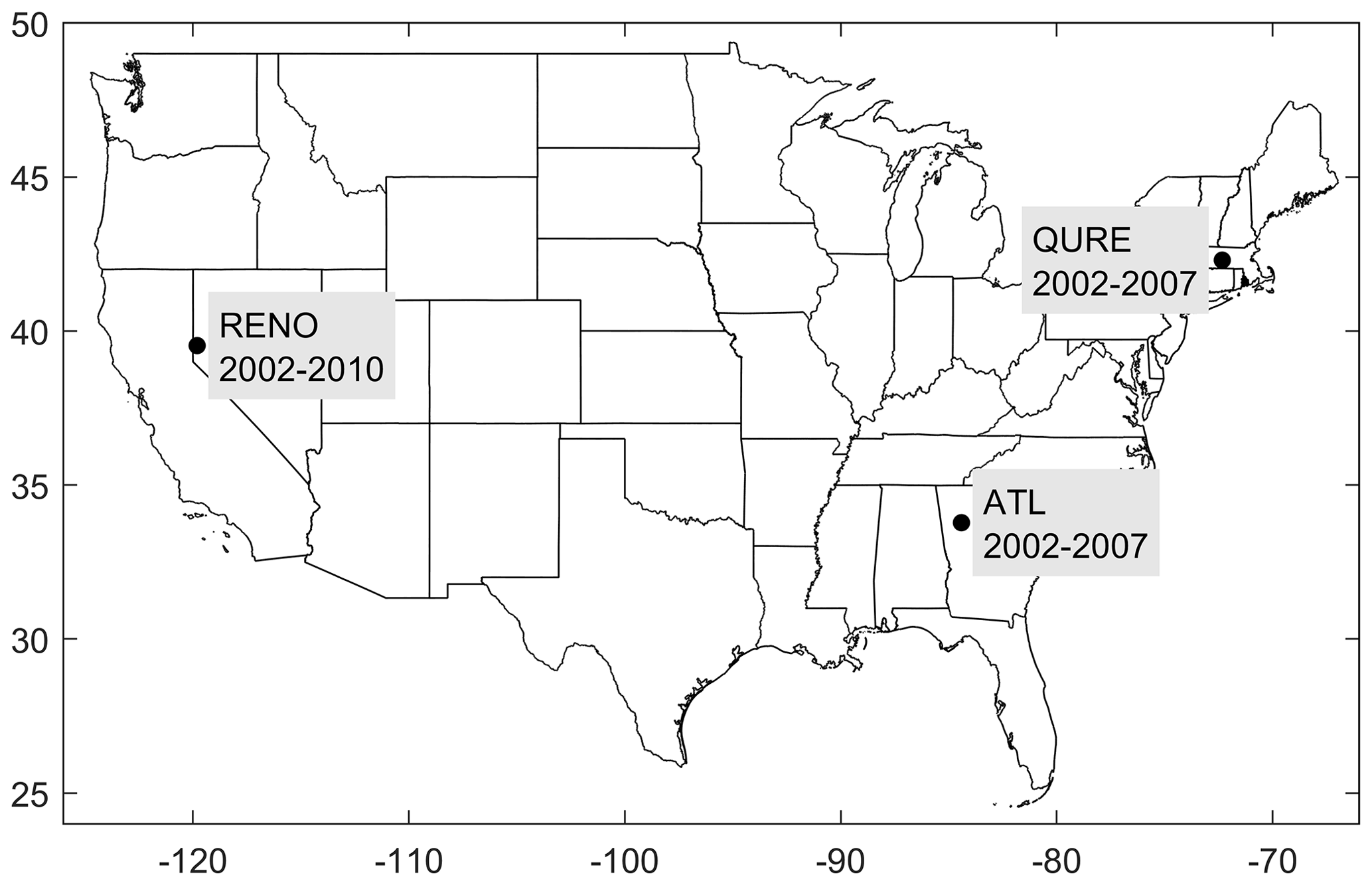
Figure 1 Location and data coverage of the PM_2.5 monitoring sites QURE, RENO, and ATL.

3 Methodology

3.1 Empirical mode decomposition

The empirical mode decomposition (EMD) technique, proposed in the late 1990s, is capable of adaptively and recursively decomposing a signal into multiple modes called intrinsic mode functions (IMFs), whereby each mode has a characteristic frequency, and a residual with one extremum at most (Huang et al., 1998). EMD decomposes the original signal into several IMFs and a residual through a repeated process called “sifting”: first, local maxima and minima are identified and interpolated separately with a cubic spline as the upper and lower envelop; then an IMF candidate is derived by subtracting the mean of the envelops from the original signal. If the candidate satisfies the following criteria (Huang et al., 1998), it is saved as the first IMF (IMF1), and the remaining portion (original signal – IMF1) is treated as a new input signal for the decomposition of the remaining IMFs; otherwise, more sifting processes should be carried out until the candidate becomes an IMF.

(1) The number of extrema (maxima and minima) and the number of zero-crossings must be equal or differ at most by 1. (2) The local mean at any point, the mean of the envelope defined by local maxima and the envelope defined by local minima, must be zero.

In this way, IMF1, IMF2, etc., are decomposed recursively with decreasing characteristic frequency. The final remaining residual (trend) could be a monotonic function of time or a long-term component with one extremum at most. The decomposed signal then is expressed as the summation of all IMFs and the final residual:

$$\begin{array}{}\text{(1)}& x={\sum }_{i=\mathrm{1}}^k{d}_i+r,\end{array}$$

where x is the original signal, d_i is the ith IMF, k is the total number of IMFs, and r is the final residual.

Nevertheless, “mode mixing”, where oscillations with very disparate scales can be present in one mode or vice versa, is commonly reported. To cope with this issue, multiple noise-assisted EMDs have been developed successively (Wu and Huang, 2009; Yeh et al., 2010; Torres et al., 2011; Colominas et al., 2014). It is evident that the latest improved complete ensemble EMD with adaptive noise (improved CEEMDAN) manages to alleviate the problem of mode mixing, with the benefit of reducing the amount of noise presented and avoiding spurious modes (Colominas et al., 2014). Moreover, the end effects or boundary effects have been addressed by its predecessor EEMD (ensemble empirical mode decomposition) by extrapolating the maxima and minima and behaved well in numerous time series with dramatically variant characteristics (Wu and Huang, 2009). The extrapolation of maxima and minima is proven to be more effective compared with the extrapolation of the signal itself such as repetition or reflection (Rato et al., 2008).

Given the EMD technique's ability to deal with real-world nonstationary and nonlinear time series, it is widely used in engineering, economics, and earth and environmental sciences (e.g., Huang et al., 1998; Chang et al., 2003; Yu et al., 2008; Colominas et al., 2014; Derot et al., 2016). We use the most up-to-date noise-assisted improved CEEMDAN technique with at least hundreds of noise realizations to decompose observed and simulated PM_2.5 time series. Readers can refer to Colominas et al. (2014) for a detailed description of the technique and access to the corresponding MATLAB code. Trial and error attempts are made in setting the inputs (standard deviation of the added noise and the limit of maximum number of sifting allowed) of the improved CEEMDAN function to achieve best mode separation. In a desired best mode separation, neighboring IMFs should have very limited levels of mode mixing, which can be fast-screened based on the time series of the decomposed IMFs and their power spectrum.

The impact of boundaries on the decomposed annual cycles and the residual is assessed by the variations (standard deviation) of hypothetical decomposed boundaries by cutting a continuous 18-year total PM_2.5 observation (North Little Rock, AR) 48 times at different years and times of the year (Fig. S1 in the Supplement). The standard deviation of the annual cycles is found to largely diminish within half the annual cycles and could be negligible within 1 year. This could very possibly expand to IMFs with other characteristic scales. Yet, trend components (residuals) show variability depending on the available time period after cutting. Most of the time, they follow the reference long-term trend reflected either by the residual or the summation of the residual and the IMF with the longest temporal scale decomposed from the 18-year PM_2.5 (Fig. S1c). This is in line with our expectations as a trend should exist within a given time span, following the definition in Wu et al. (2007): “The trend is an intrinsically fitted monotonic function or a function in which there can be at most one extremum within a given data span”.

Although a very strict data completeness requirement is employed for this study, it should not be conceived as a limitation of the method itself. A sensitivity test based on a period of 9 years of total PM_2.5 observations at the same site with 99 % data coverage shows that even though variability of annual cycles and long-term trends increases with decreased data availability (100 %, 90 %, …, 10 %), the structure of those components is consistent. The average of 40 realizations of annual cycles and long-term trend components in each data completeness scenario is in perfect alignment with that of 100 % data completeness (Figs. S2 and S3). Given the fact that those 40 realizations in each scenario are based on independent random samplings of the original observations, the increased variability could very possibly result from the difference in the sampled data itself rather than the method. Thus, the robustness of the improved CEEMDAN decomposed annual cycles and long-term trend is justified. In fact, EMD has been proven to be an effective tool for data gap-filling (Moghtaderi et al., 2012).

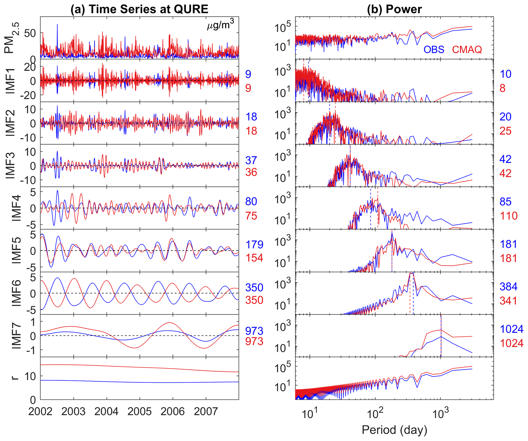
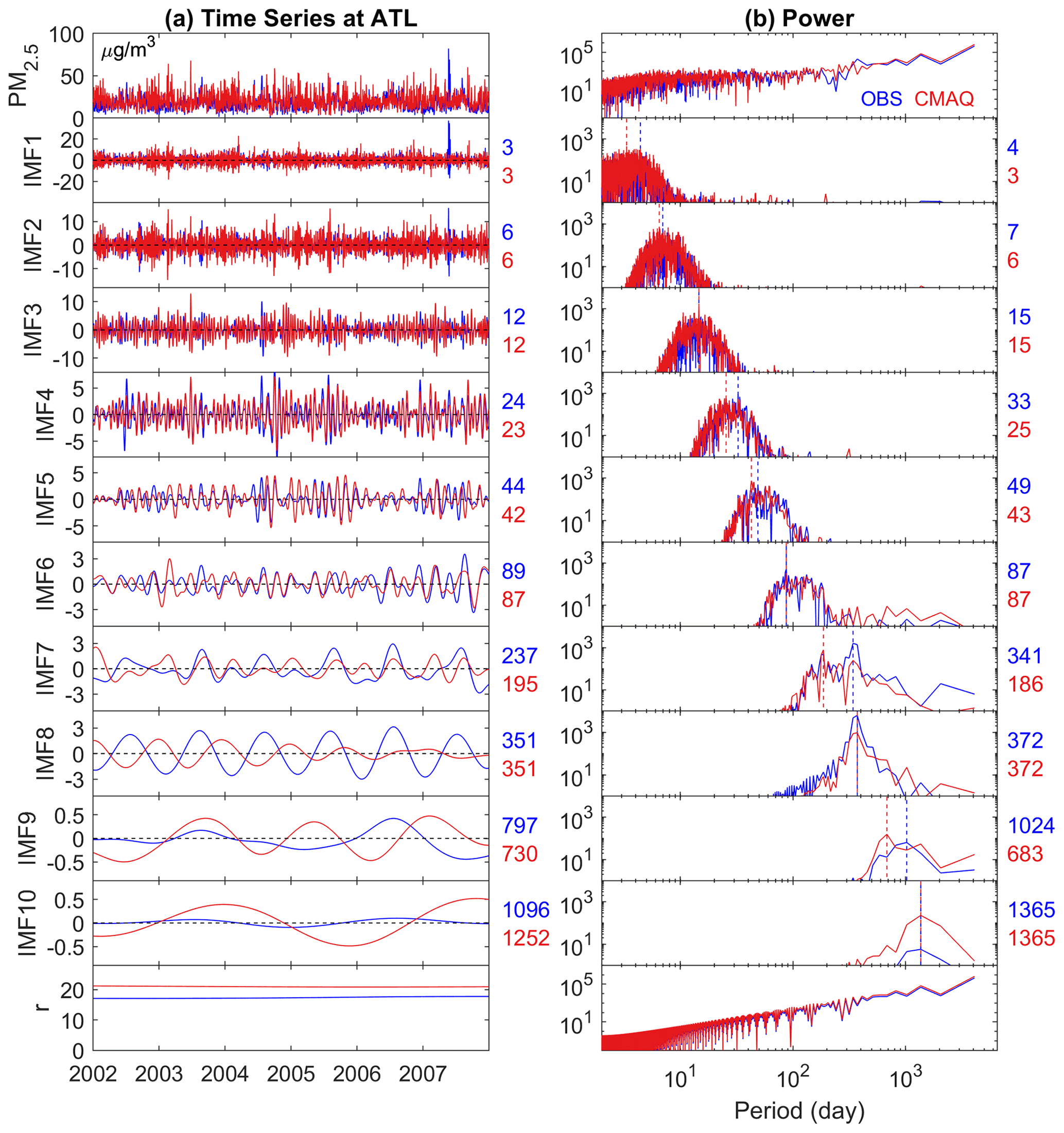
Figure 2 Decomposition of observed (blue) and simulated (red) 24 h average total PM_2.5 into seven IMFs and a residual component (trend) at Quabbin Summit, MA, using the improved CEEMDAN: (a) time series of total PM_2.5, IMFs, and the residual component (all in units of micrograms per cubic meter; µg/m³); (b) power spectrum of the corresponding time series. The colored numbers on the right side of the time series are the mean period t_m in days, while the ones on the right side of the power spectrum are the peak period =t_p in days, which are also indicated by the dashed vertical lines on the power spectrum. Note that the scales for the time series are not all the same. Also, all power spectra are on the log scale, and those of the IMFs are zoomed in at a range of 10⁰ to 10⁴ on the y scale for better visual clarity (compared with 10⁻² to 10⁷ for total PM_2.5 and the residual component).

The characteristic period of each IMF can be estimated by the peak period t_p (days) where the power spectrum of the IMF peaks:

$$\begin{array}{}\text{(2)}& t_{\mathrm{p}}={\displaystyle \frac{\mathrm{1}}{f_{\mathrm{p}}}},\end{array}$$

in which f_p is the frequency that the power spectrum peaks in units of number of cycles per day. The peak estimates can be biased if more than one high-power frequency is located closely within one IMF. Thus, the power spectrum and t_p are only used as a fast screening tool to determine if a desired decomposition is accomplished. As an alternative approach, the mean period t_m can be estimated by

$$\begin{array}{}\text{(3)}& t_{\mathrm{m}}={\displaystyle \frac{\mathrm{Time}\mathrm{span}}{(n_{\max }+n_{\min }+n_{\mathrm{zero}})/\mathrm{4}}},\end{array}$$

where n_max , n_min, and n_zero are the number of maxima, minima, and zero-crossings, respectively, during the time span (days). As the frequency decreases, the mean period estimates become less accurate because of the limited time span compared with the length of the cycle and should be carefully interpreted.

An example of the total PM_2.5 decomposition with improved CEEMDAN at the QURE site shows modes ranging from very high frequency to very low frequency (IMF1 to IMF7) and a residual (Fig. 2). No visible mode mixing can be detected in both the time series (Fig. 2a) and the power spectrum (Fig. 2b) of all IMFs. Mean (t_m) and peak (t_p) estimations of the characteristic periods of each IMF are presented on the right side of each mode. Annual cycles and long-term trend components are well represented by IMF6 and the residual, with the remaining IMFs carrying weekly, sub-seasonal, seasonal, and interannual variations, respectively, for both observed and simulated PM_2.5 (Fig. 2). We have noticed that in some rare cases, a spurious mode in the last IMF with synchronous signal and very close scales to its previous IMF exists. This is possibly due to the fact that the characteristic periods of those IMFs are in proximity to the span of the studied time span. In these cases, the last two modes are merged by adding them together to conduct a detailed evaluation as discussed in Sect. 4.1.

3.2 Statistical metrics

EMD-decomposed IMFs and trend components allow for a detailed time-dependent evaluation of PM_2.5 and provide a novel opportunity to trace the performances of specific scales back to the corresponding speciated components. Note that the trend component is the decomposed residual component from the PM_2.5 in units of micrograms per cubic meter (µg/m³), and it is not the traditional concept of trend in concentration per time. In addition to a direct evaluation of its magnitude, we also calculated its derivative to identify the periods with higher or lower rate of change (concentration per time). Time-dependent intrinsic correlation (TDIC) is utilized to study the evolvement of the model performance for cyclic variations throughout time (Chen et al., 2010; Huang and Schmitt, 2014; Derot et al., 2016). It is a set of correlations calculated for IMFs over a local period of time I centered around time t:

$$\begin{array}{}\text{(4)}& I\left(t\right)=\left[t-{\displaystyle \frac{t_{\mathrm{w}}}{\mathrm{2}}}t+{\displaystyle \frac{t_{\mathrm{w}}}{\mathrm{2}}}\right],\end{array}$$

in which t is the center time for the calculation of the correlation, and t_w is the moving window length. The minimum of t_w is set to be the local instantaneous period of the IMF (larger of that in observation or simulation) using the general zero-crossing method to ensure that at least one instantaneous period is included in calculating the local correlation coefficient (Chen et al., 2010). The maximum of t_w is the entire data period with a traditional overall correlation being calculated. The empty spaces in the pyramids used to depict the TDIC are an indication that the correlation is not statistically significantly different from zero. With both decomposed observed and modeled concentrations in a narrow scale range, the correlation would no longer be contaminated by coexisting signals of different scales (Chen et al., 2010).

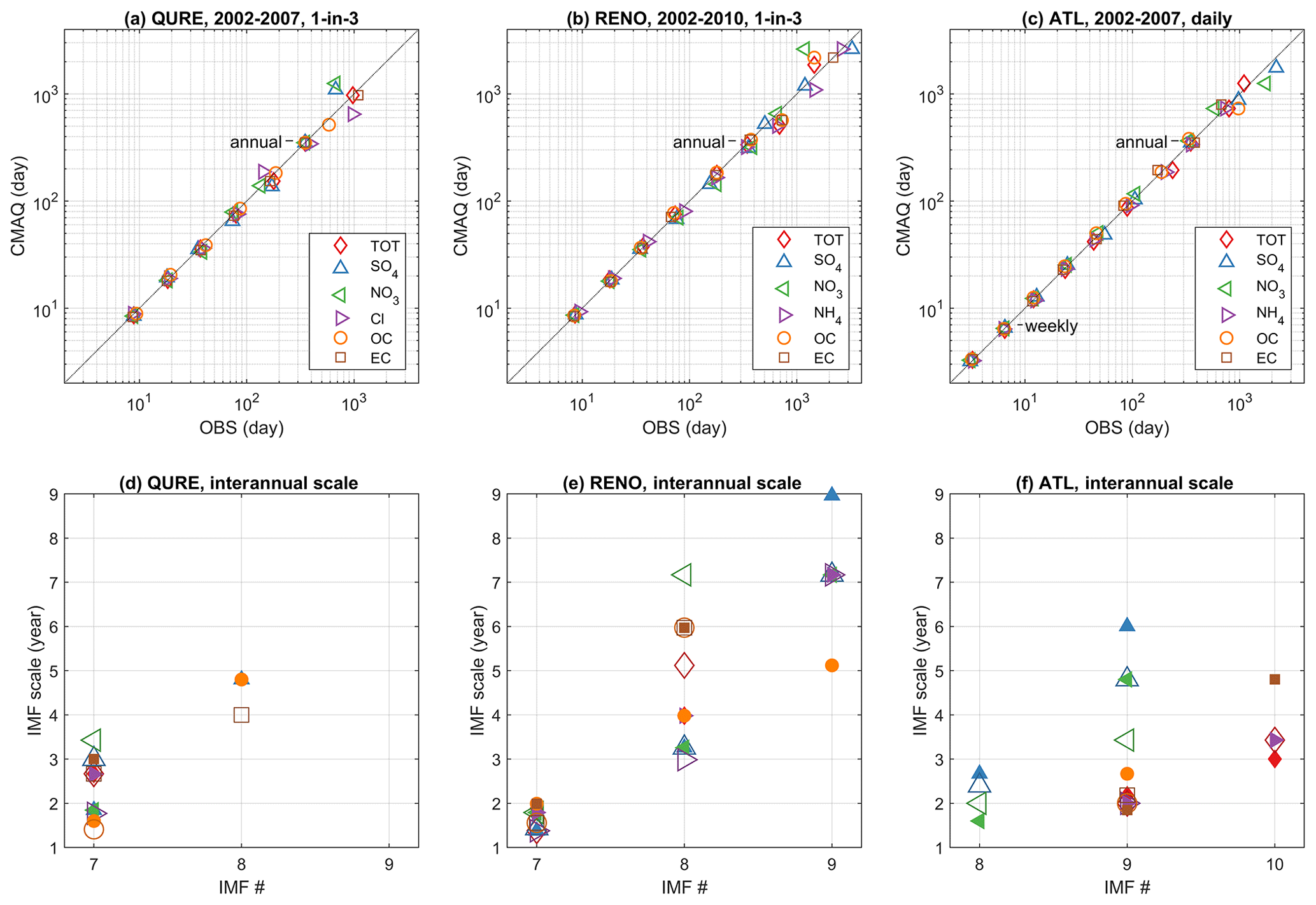
Figure 3 The characteristic scales (t_m) resolved in the IMFs of observed and simulated total and speciated PM_2.5 for (a, d) QURE, (b, e) RENO, and (c, f) ATL. In (a–c), IMF1 to the last pair of IMFs with increasing characteristic periods are shown from the bottom left to top right. Mean periods of IMFs with scales longer than a year are displayed in (d–f) with the same shapes as in the legend above to show the characteristic scales of all decomposed IMFs given that not all IMFs from the observation are being simulated and vice versa. In (d–f), species decomposed from observations are shown with smaller filled shapes, while species decomposed from simulations are represented by larger open shapes in slightly darker shades.

In order to summarize the performance of the decomposed trend components and IMFs, the ratio of the mean magnitudes of the trend components is defined as

$$\begin{array}{}\text{(5)}& r_{\mathrm{trend}}={\displaystyle \frac{{\mathrm{Mean}}_{\mathrm{CMAQ}}}{{\mathrm{Mean}}_{\mathrm{observation}}}},\end{array}$$

where Mean_CMAQ and Mean_observation represent the mean of simulated and observed residual components respectively. The ratio of the mean amplitude of each IMF is defined by Eq. 6, in which an example for the annual cycles is provided:

$$\begin{array}{}\text{(6)}& r_{\mathrm{annual}}={\displaystyle \frac{{\mathrm{RMS}}_{\mathrm{CMAQ},\mathrm{annual}}}{{\mathrm{RMS}}_{\mathrm{observation},\mathrm{annual}}}},\end{array}$$

where RMS_{observation, annual} and RMS_{CMAQ, annual} represent the root mean square of observed and simulated annual cycles respectively. Finally, the phase shift of an IMF n is defined as the days an IMF decomposed from modeled time series has to be shifted to maximize the correlation (R_max) with the corresponding IMF from observed PM_2.5 time series. In practice, n could be as much as a few cycles of the mean period, t_m. Here, we limit the absolute number of shift days to not exceed a half cycle as a reference for the phase shift of an IMF. Thus, n satisfies $-\left(t_{\mathrm{m}}/\mathrm{2}\right)\le n\le$ (t_m∕2), with t_m being the larger mean period in the observation or simulation. It becomes $-\mathrm{0.5}\le n/t_{\mathrm{m}}\le \mathrm{0.5}$ in terms of number of cycles.

4 Results and discussion

4.1 Temporal scales

Temporal scales in PM_2.5 resolved by EMD depend solely on the intrinsic properties of the data itself. These properties include underlying characteristics of specific PM_2.5 concentrations, the data sampling frequency, which determines the scales that can be resolved in the high-frequency IMFs, and the time span for the data coverage, which could possibly play an important role in differentiating the low-frequency IMFs from the trend component. Here, we first evaluate the scales represented by the mean period in the speciated and total PM_2.5 time series. Since each IMF represents a nonstationary process, the mean period t_m is only an estimate of its characteristic scale. Evaluation of t_m might not necessarily be able to identify issues with corresponding model simulations, and it does not indicate any information on the magnitude or the phase of the time series, which is more important and will be further discussed in Sect. 4.3 to 4.4.

Figure 3a presents the characteristic scales (t_m) of IMFs in observed and simulated total and speciated PM_2.5 of QURE. The CMAQ model compares well with the observations for IMFs 1 through 6, with cycles of 9, 19, 37, 78, 158, and 347 d (average of all observed and simulated total and speciated PM_2.5). Among all these IMFs, IMF6, which represents the annual cycles, shows the least variation on the characteristic scale (Fig. 3a) and highest peak energy from the power spectrum such as Fig. 2b for total PM_2.5, except for observed EC and OC where the power of half-year cycles is more dominant (Fig. S4). These two features demonstrate a clear seasonality in both observed and simulated total and speciated PM_2.5, which would otherwise be concealed by practices such as monthly averaging. This can be further confirmed by the statistical significance of the annual cycles (except for observed EC and OC; Fig. S5) based on a Monte Carlo-verified relationship between the energy density and mean period of IMFs (Wu and Huang, 2004; Wu et al., 2007). To explore the interannual cycles in more detail, mean periods of IMFs with scales longer than a year are displayed in Fig. 3d. Some variability exists between the observation and model simulation to the extent that not all IMFs from the observation are being simulated and vice versa for the interannual cycles. The estimated mean periods of the interannual cycles and the differences in the presence of slow varying cycles with the long characteristic scales are likely to be influenced by their proximity to the data time span of 6 years (4 years for Cl). This implies that the model evaluation should not go beyond 3 years (2 years for Cl) given the current data coverage. CMAQ captured the 3-year cycles in EC and total PM_2.5 and 2-year cycles in OC and Cl, despite an overestimation in the scales of 2-year cycles in observed SO₄ and NO₃.

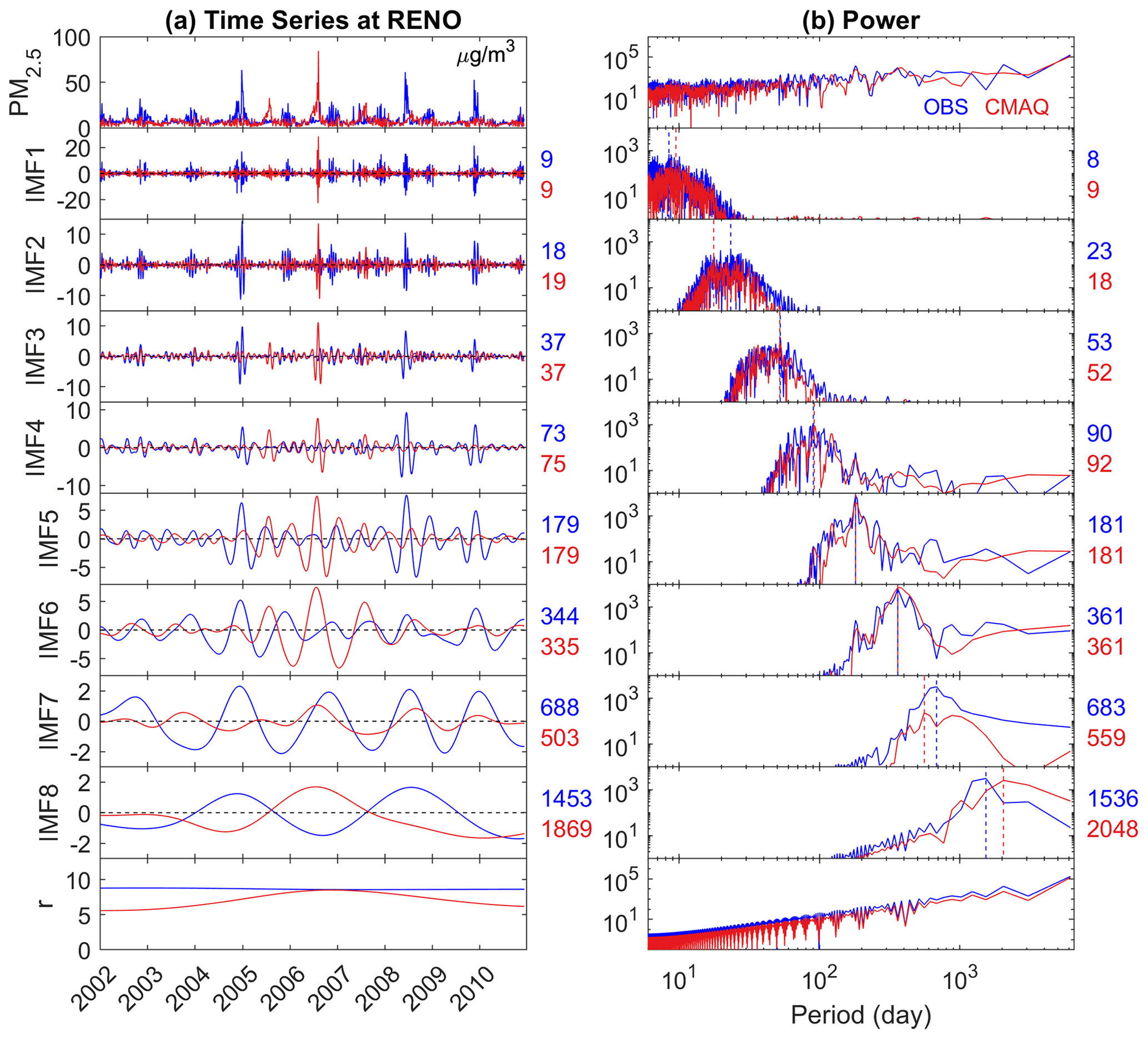
Similar features in observed and simulated total and speciated PM_2.5 concentrations at RENO are presented in Fig. 3b. Likewise, the highest peaks in the power spectrum are also in the annual cycles of IMF6 except for the observed OC and total PM_2.5 which have higher peak power in the half-year cycles. All annual IMFs are statistically significant except for simulated NH₄ (Fig. S5). The small variation in the estimated characteristic period of IMF6 is because this monitoring site is located in a wildfire-prone region on the border of Nevada and California. Clear evidence can be seen from Fig. 4a that an extra annual cycle in the IMF6 of observations in the summer of 2008 is depicted, which is very possibly driven by the 2008 California wildfires spanning from May until November. A satellite image of the wildfire smoke on 10 July 2008 can be found in Fig. 1 of Gyawali et al. (2009). Unlike the diversified scales in IMF7 at QURE, IMF7 at RENO features universal 2-year cycles of all species as well as total PM_2.5, and all of them are well replicated by the model. However, variations in timescales are present in IMF8, possibly because of the limited data coverage. Thus, only species with timescales less than 4 years in both observations and model simulations are evaluated. It is evident that CMAQ has reproduced the 3-year cycles in SO₄ and NH₄.

ATL is the only speciated site with daily data coverage. Observed and simulated total and speciated PM_2.5 concentrations at the ATL site are decomposed into 9 or 10 IMFs (Fig. 3c). Because of the change in data frequency, high-frequency scales such as weekly cycles can be evaluated and the significance tested (Fig. S5). Annual cycles of total PM_2.5 are represented by IMF8 (IMF7 for SO₄ and NO₃) which have passed the test for statistical significance (available in Fig. S5). Annual cycles of SO₄ and NO₃ appeared in the earlier stage of decomposition in IMF7 because of their relatively weak half-year cycles, which largely led to the mixed signal of half-year and annual cycles in IMF7 in total PM_2.5 as in Fig. 5b. This is more visible in the observed IMF7, in which the energy of the 1-year period surpasses that of the half-year. Yet, clues can be seen from Fig. 5 that the amplitude and the energy of annual cycles leaked into IMF7 are very limited compared to what remains in IMF8, indicating that it is still safe to conduct model evaluation on the seasonality using IMF8 with an underestimation in the amplitude of observation. On the other hand, inferences should be made with caution for IMF7 because of the mixed modes. Scales up to 3 years are relatively well reproduced by the model.

Figure 4 Same as Fig. 2 but for the RENO site with 8 IMFs.

Figure 5 Same as Fig. 2 but for the ATL site with 10 IMFs.

4.2 Long-term trend

The EMD-decomposed long-term trend components for the observed and simulated total and speciated PM_2.5 concentrations are presented in Fig. 6. To better visualize the non-linearity of the trend component, the rates of change (temporal derivative of a trend component, which is the change in the consecutive concentration divided by the sampling period of 1 or 3 d and converted to units of micrograms per cubic meter per year, µg/m³/year, by multiplying it by 365 days per year, 365 d/year) are added with a separate y axis on the right side of each panel (gray-colored scale). It is evident that PM_2.5 is changing at a varying rate, forming either a monotonic trend component or a trend component with one extremum, which cannot be fully represented by a single constant number using a traditional linear regression approach. Given that there are chemical species (the remaining component, “Rem”) other than the ones studied in the total PM_2.5, not all performance issues can be fully explained by the five available species.

At the QURE site, CMAQ captures the general decreasing trend in observed total PM_2.5 which can mainly be traced back to NO₃, OC, and the remaining components, while both observed and simulated trend components of SO₄ and EC are relatively constant (Fig. 6a). The relative importance of each component in driving the trend of observed and simulated total PM_2.5 reflected by its mean concentration share is summarized in Table 1 (time-dependent variations of the concentration share are attached in Fig. S6 for reference). Moreover, the periods with the highest decreasing rate in observed total PM_2.5 during 2003–2004 with a decreasing rate of −0.44 µg/m³/year are also well replicated by the model. Nevertheless, the slightly increasing PM_2.5 level in the later years is simulated to be decreasing at a much higher rate, which is partly due to the overestimated decreasing rate in OC and species other than the five studied ones. The trend component of simulated Cl shows a cyclic-like feature because of proximity between the existence of a cycle of 4–5 years (by decomposing the simulation during the 6-year study period) and 4-year period limited by the available quality-assured observations. The rate of change in the simulated trend component by decomposing the simulation during the 6-year study period would mimic that of the 4-year observation, both with a negligible negative value throughout 2004–2007. However, the mean magnitude of the trend component is almost twice as high (1.8 times compared with observations) in the model, with contribution from all species except for SO₄. A quantitative summary of the comparison between the mean magnitudes of the observed and model trend components can be found in Table 2.

RENO is located close to the border with California and is affected by large wildfire breakouts in the western United States (Gyawali et al., 2009) as can be seen in the spikes of the observed total PM_2.5 (Fig. 4a). Thus, OC makes up a much larger portion of total PM_2.5 compared to other locations (Table 1). The model simulates a large increasing rate of up to 1.03 µg/m³/year and a decreasing rate of up to −0.80 µg/m³/year before and after the 2006–2007 winter season and fails to reproduce the relatively stable condition seen in the observations with only −0.09 µg/m³/year decreasing rate in 2004–2005 and 0.04 µg/m³/year increasing rate in 2008–2009 (Fig. 6b). A similar feature is found for combustion-related OC and EC species. The observed slightly decreasing trends in SO₄ and NH₄ during 2005–2009 are not being captured in the model simulations. The magnitude of the trend component is slightly underestimated, with r_trend of 0.8, with contribution from all species except for SO₄ as well (Table 2).

During the period of 2002–2007, observations at ATL reveal a slightly increasing PM_2.5 trend that cannot be explained by the five available PM_2.5 components' trend (Fig. 6c), indicating a contribution of the remaining species such as the non-carbonaceous portion of organic matter. Non-carbonaceous organic matter can account for more than half of total organic matter, which, in turn, can account for a large portion of the total PM_2.5 mass (Edgerton et al., 2005). In contrast, the model shows a slight decreasing trend with a peak decreasing rate in 2003 and misses the peak increasing rate of 0.23 µg/m³/year in the winter season of 2005. Similarly, reversed trends are also simulated for SO₄, OC, and EC, while the change rate in NO₃ is well captured. Unlike the previous sites, the magnitude of trend components in total and speciated PM_2.5 is well simulated except for EC (1.4 times the observation) and NO₃ (2.1 times).

To sum up, the decreasing long-term trend at QURE is well simulated by the model. The occurrence of large wildfires lasting for several months has significantly impacted the long-term trend component at RENO, and the model failed to capture these combustion-related species and total PM_2.5, primarily due to limitations in the historical data used to specify day-specific wildfire emissions (Xing et al., 2013). Slightly increasing levels of PM_2.5 and its species observed at ATL are simulated to be slightly decreasing, except for NO₃ which is well simulated. The magnitude of the long-term trend components of total PM_2.5 and SO₄ is well represented by CMAQ (Table 2). The model performs differently across the sites in terms of the magnitudes of the trend component in NO₃, NH₄, Cl, OC, and EC. The large discrepancy in the magnitude of some long-term trend components likely points to the systematic bias in the annual emission estimations as discussed in Xing et al. (2013), which mainly focused on the long-term trend rather than the absolute level of the emissions. Species other than those in the available dataset also play a considerable role in driving the agreements or disagreements between model simulations and observations of total PM_2.5.

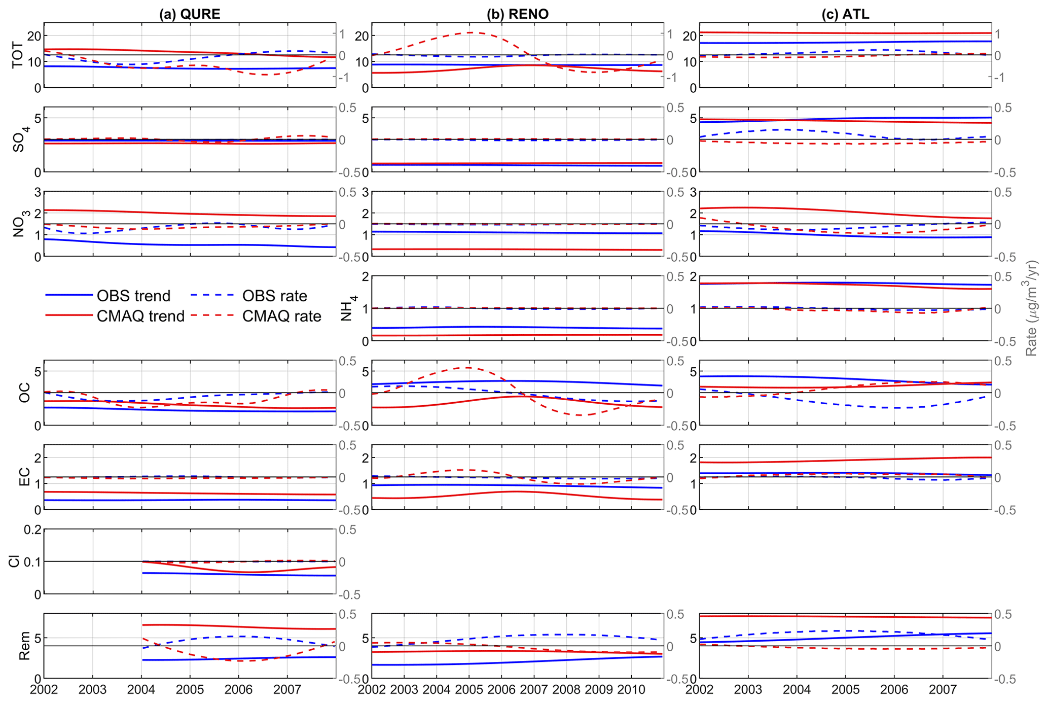
Figure 6 Trend components of observed and simulated total and speciated PM_2.5 for (a) QURE, (b) RENO, and (c) ATL in micrograms per cubic meter (µg/m³). Dashed lines representing the rate of the change (temporal derivative of the trend component converted to µg/m³/year) are plotted against the right-side y axis, with a reference line of no change in black in the center. Note that the scales are not all the same.

Table 1 Concentration share (%) of different components in total PM_2.5. It is estimated by dividing the mean trend components of each species by that of total PM_2.5 for both OBS and CMAQ, multiplied by 100. The concentration share of the remainder species, Rem, is estimated by subtracting all the available species' share from 100 to compensate for the small discrepancies caused by the rounding up process and uncertainty in the mode decomposition. “–” indicates the data are not available (same applies for all other tables).

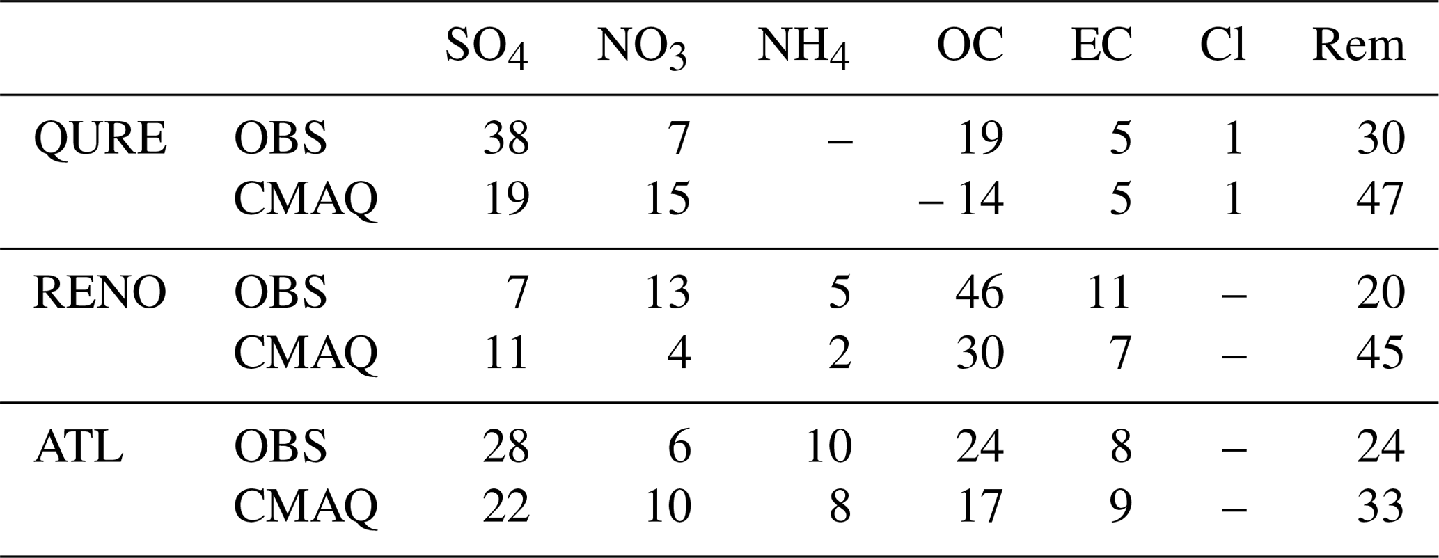
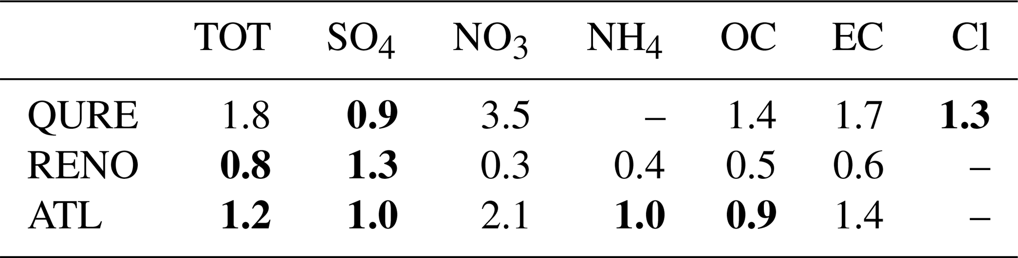
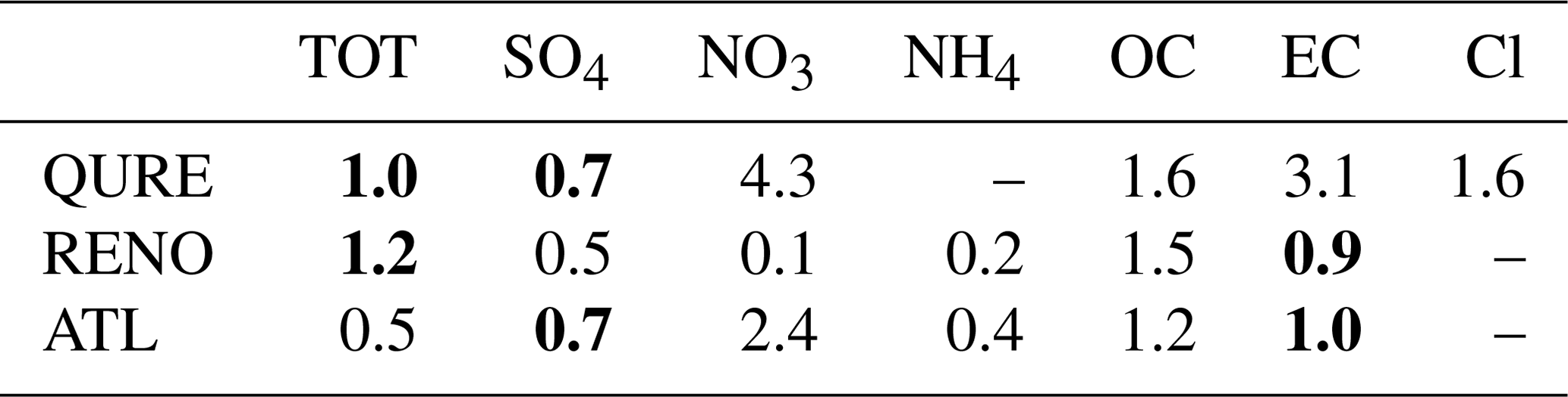
Table 2 The ratio of mean magnitude of the trend component r_trend (CMAQ/observation). Boldface values indicate a relatively good estimate of the magnitude (0.7–1.3).

4.3 Seasonality

The EMD-assisted seasonality evaluations utilize the decomposed IMFs with a characteristic period of 1 year to evaluate the amplitude and phase of the model simulation, both of which are time-dependent. As mentioned in Sect. 4.1, these IMFs are statistically significantly different from white noise with few exceptions (Fig. S5). We first demonstrate the evaluation for total PM_2.5 at QURE (Fig. 7a). The top panel shows the annual cycle components, and the bottom panel shows its TDIC pyramid. The decreasing amplitude of the annual cycles throughout 2002–2007 is almost perfectly represented, with an overall ratio r_annual of 1.0 (Table 3). Each pixel in the TDIC pyramid is the correlation (color-coded) calculated during a period of time I(t) with width of t_w days (y axis) centered at a specific day (x axis) as introduced in Sect. 3.2. The annual cycle mean periods are identical between CMAQ and observations (350 d, Fig. 2a IMF6), but there is a phase shift for all years, with the entire TDIC pyramid being close to −1. By shifting the CMAQ annual cycles backward 159 d (almost half a year), the overall correlation of the annual component can reach up to a peak of 0.9 (Table 4).

What are the driving factors for the above phase shift in modeled total PM_2.5 at Quabbin Summit, MA? The illustrations in Fig. 7a for total PM_2.5 alone cannot provide useful information that will allow the modeler to improve the model's performance. This is accomplished by applying the EMD method to the PM_2.5 speciated components (Fig. 7b–f). Traces of the semi-annual phase shift (−159 d) of annual cycles or the large overestimation in the winter and underestimation in the summer are because of the largely overestimated amplitude of NO₃ (4.3 times that of observation) which peaks in the winter and the almost semi-annual shifted OC (−147 d), as well as contributions from EC and Cl. NO₃ has a mean amplitude reaching almost half of that of the total PM_2.5. OC directly drives both the observed and simulated annual components to be negatively correlated. EC follows the feature of OC in the first 4 years or so, and the feature of NO₃ in 2006 and 2007 and contributes to the half-year-shifted total PM_2.5. The magnitude of winter-peaking Cl cycles is overestimated, with a phase shift of 1 month. However, the contribution of Cl is very limited because of the tiny amplitude in both observed and simulated annual cycles. In addition, annual cycles in SO₄ are well reproduced for the entire time span, with an amplitude ratio of 0.7. A quantitative summary of the evaluation of the annual cycles at this site can be found in Tables 3 and 4.

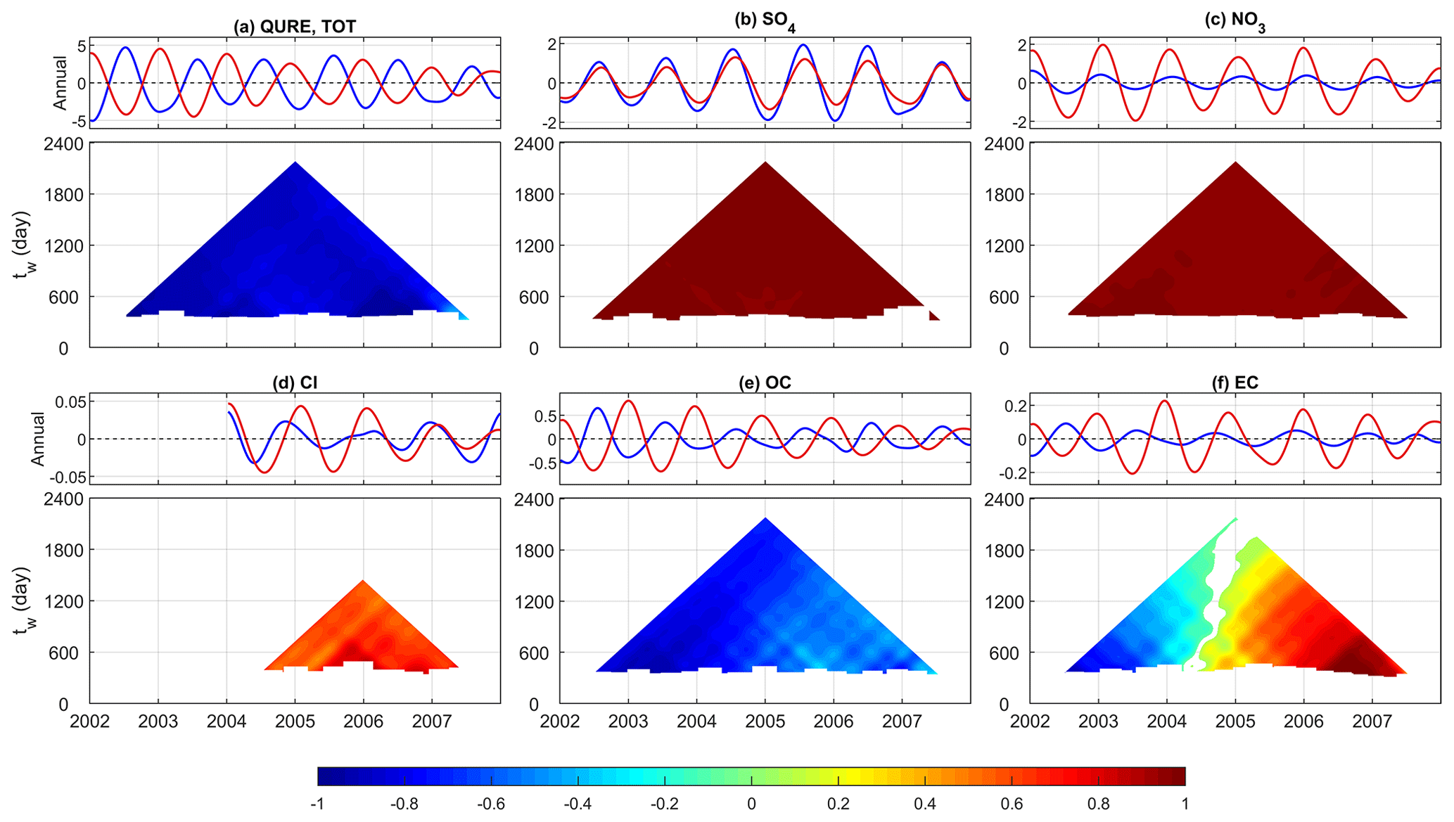
Figure 7 Decomposed annual cycles (IMF6) from observed (blue) and simulated (red) concentrations (µg/m³) of (a) total PM_2.5, (b) SO₄, (c) NO₃, (d) Cl, (e) OC, and (f) EC and their corresponding TDIC at Quabbin Summit, MA. The window size t_w indicates the width of the window used to calculate a specific correlation centered at the day represented on the x axis.

Figure 8 Same as in Fig. 7 for Reno, NV, except that (d) represents NH₄ rather than Cl.

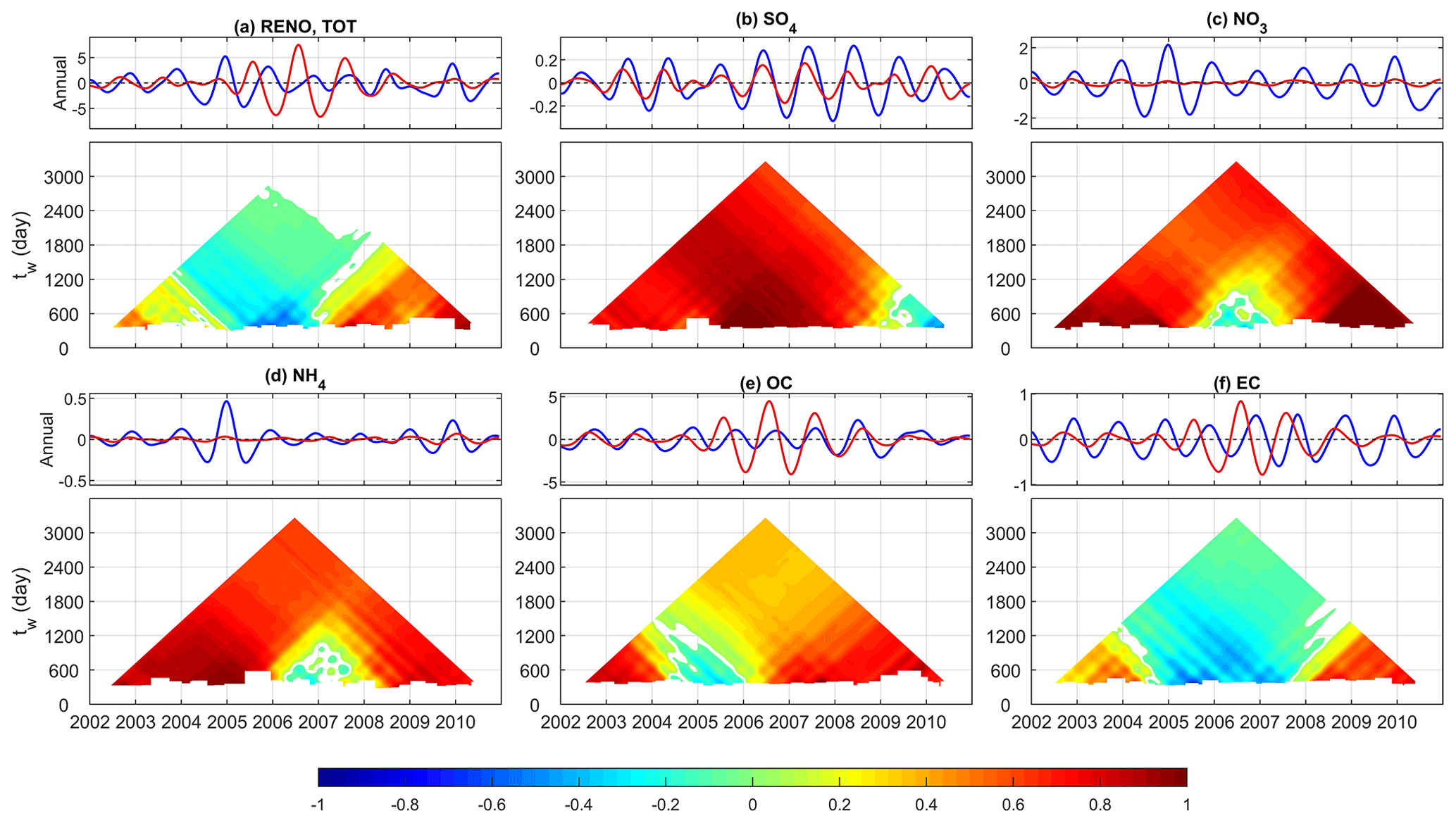
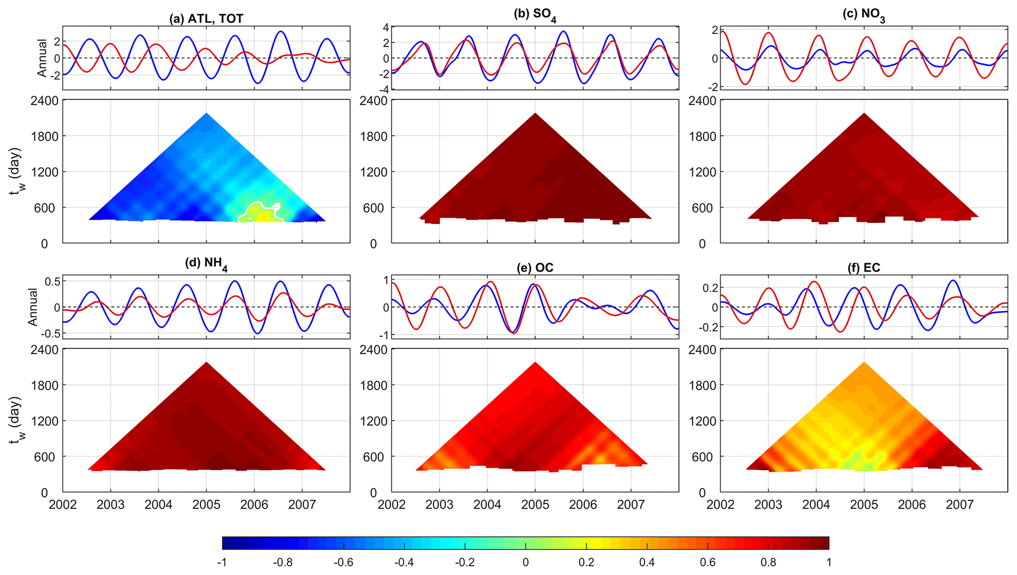
Figure 9 Same as in Fig. 7 for Atlanta, GA, except that the annual component is resolved in IMF8 (IMF7 for SO₄ and NO₃) because of the difference in sampling rate and characteristics embedded in the time series at ATL, and (d) represents NH₄ rather than Cl.

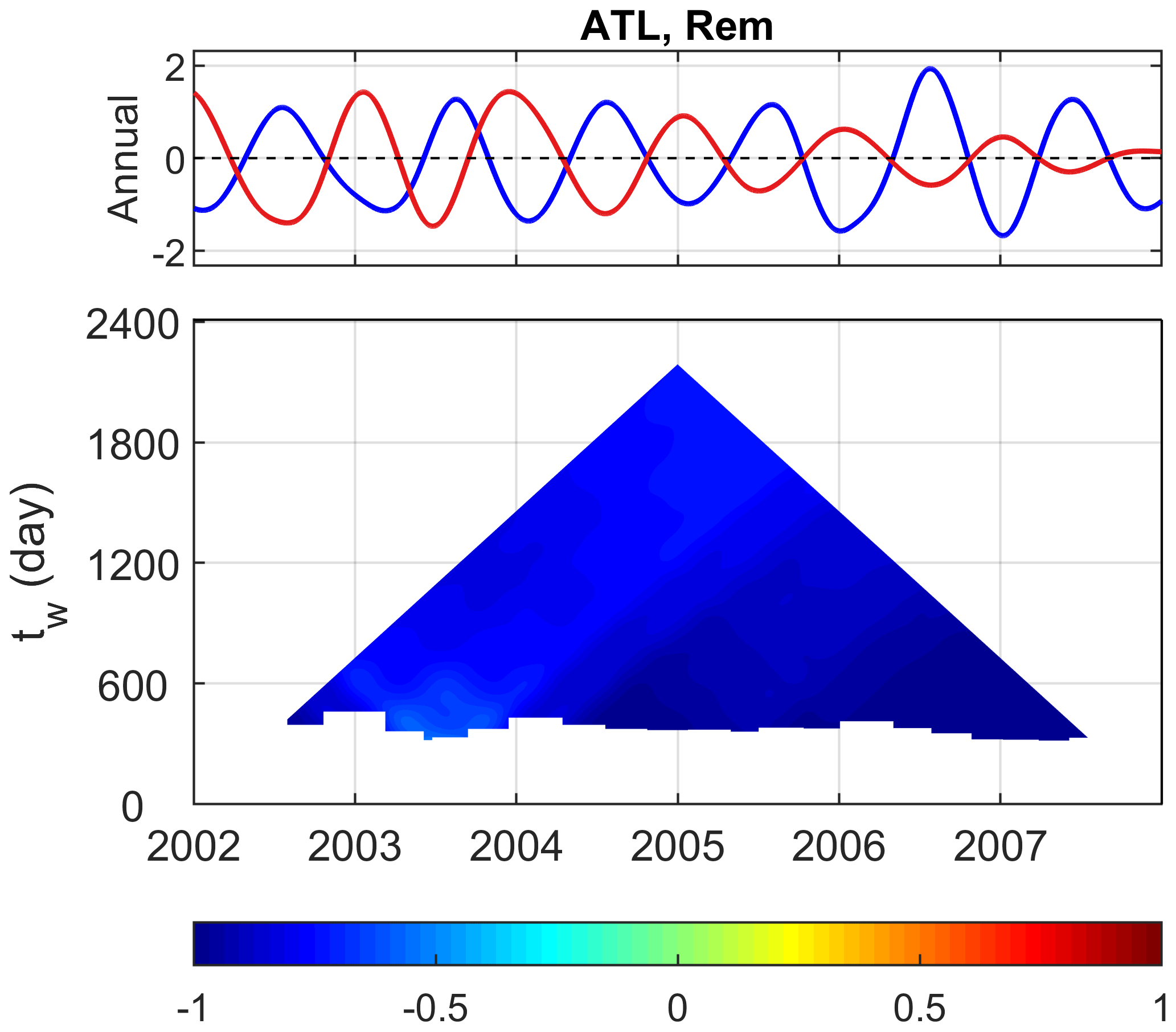
Figure 10 Decomposed annual cycles in Atlanta, GA, for the remaining components presented in total PM_2.5 other than the five species in Fig. 9.

Both observed and simulated annual cycles at the RENO site are largely influenced by the extreme events lasting for several months that are not properly simulated, indicating the need for more accurately specified wildfire emissions. Overall, annual variations for total and speciated PM_2.5 are largely underestimated except for the total PM_2.5 and combustion-driven EC and OC from 2005 to 2007 (Fig. 8). The modeled phase of SO₄, NO₃, NH₄, and OC agrees with that of observation with the exception for a length of about 2 years in each that missed the phasing: 2009–2010 for SO₄, summer 2005–summer 2007 for NO₃, 2006–2007 for NH₄, and 2004–2005 for OC. It is also notable that the TDIC pyramid of EC mimics that of total PM_2.5, implying the existence of errors in modeled EC in processes such as emissions, transport, and deposition that affected the model performance for total PM_2.5. In comparison, SO₄ and OC are relatively well simulated, with a mean amplitude ratio of 0.5 and 1.5 and a phase shift of 36 and 33 d, respectively.

Observed annual cycles of total PM_2.5 at the ATL site feature a slightly increasing amplitude of annual variations from 2002 to 2006, which then decreased to the original state in 2007 (Fig. 9a). Conversely, model-simulated annual cycles became weaker throughout the period, with an overall r_annual of 0.5. As at the QURE site, the simulated annual components at the ATL site also show a shift of several months (−132 d). Specifically, traces of these phase shifts or large overestimation in the winter and underestimation in the summer can be seen from the more than doubled amplitude of NO₃ which peaks in winter and underestimated SO₄ and NH₄ in the warm seasons as well as the −54 d shifted EC. The anti-correlated remaining species other than those in the available dataset clearly played a role in driving the discrepancies seen in the total PM_2.5 annual cycles (Fig. 10). Specifically, the anti-correlation likely points to an inaccurate representation of the seasonal variation of the non-carbonaceous portion of organic matter due to an incomplete representation of organic aerosols in the model version analyzed here; newer versions of the CMAQ model include updated treatment of organic aerosols (e.g., additional secondary organic aerosol (SOA) formation pathways, improvements in representation of primary organic matter (OM) emissions), which is likely to improve the mentioned features (Appel et al., 2017; Murphy et al., 2017; Xu et al., 2018). The underestimated annual variations in the remaining components closely resemble those of the annual variation in total PM_2.5. The phase of simulated SO₄, NO₃, NH₄, and OC species is in good agreement with that in observations, and the amplitude of simulated annual cycles in SO₄, OC, and EC agrees well with that in the observations (Tables 3 and 4).

In sum, annual cycles of PM_2.5 are also time-dependent, and the phase in the annual cycles for total PM_2.5, OC, and EC reveals a general shift of up to half a year (Table 4); this indicates a potential problem in the allocation of emissions during this study period and/or the treatment of organic aerosols in this version of the model. CMAQ generally simulated the phase in SO₄, NO₃, Cl, and NH₄ quite well but did not always capture the magnitude of their variations (Table 3).

Table 3 The ratio of mean amplitude of the annual component r_annual (CMAQ/observation). Boldface values indicate a magnitude with a ratio close to 1 (0.7–1.3).

4.4 Sub-seasonal and interannual variability

In this section, model performance at multiple sub-seasonal and interannual scales with cycles less than 3 years, presented in the total and speciated PM_2.5, is evaluated following an approach similar to that for the annual cycles in Sect. 4.3 (Fig. 11). First, IMFs from observations and model simulations are paired based on their characteristic periods following the discussion in Sect. 4.1. Then, the magnitude of specific scales is evaluated using r_IMFn following Eq. 6 of the r_annual for annual cycles. The phase shifts of the time series are assessed by the proportion of shifted days relative to the mean characteristic scales of the corresponding observed and simulated IMFs (n∕t_m). For example, a phase shift of 0.1 cycles in the 2-year cycles is approximately 73 d, while it would be 18 d for the half-year cycles.

Table 4 Phase shift (n) of CMAQ-simulated annual cycle components in days. The bold font shows the number of shifts of less than a month, while the italics show shifts of longer than 3 months.

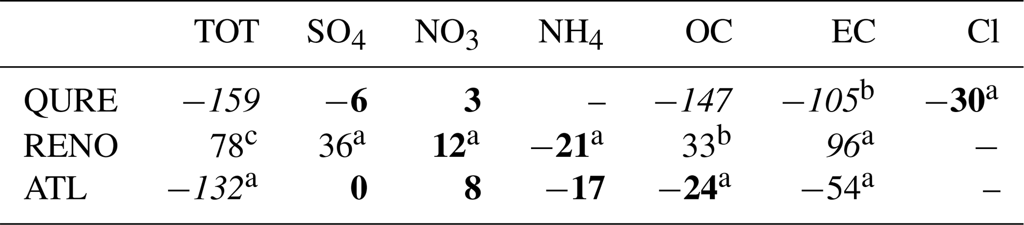
The superscripts indicate the maximum correlation (R_max) that can be reached by shifting the CMAQ time series n days with respect to observations: no superscript denotes [0.8, 1], ^a [0.6, 0.8), ^b [0.4, 0.6), and ^c (0.2, 0.4).

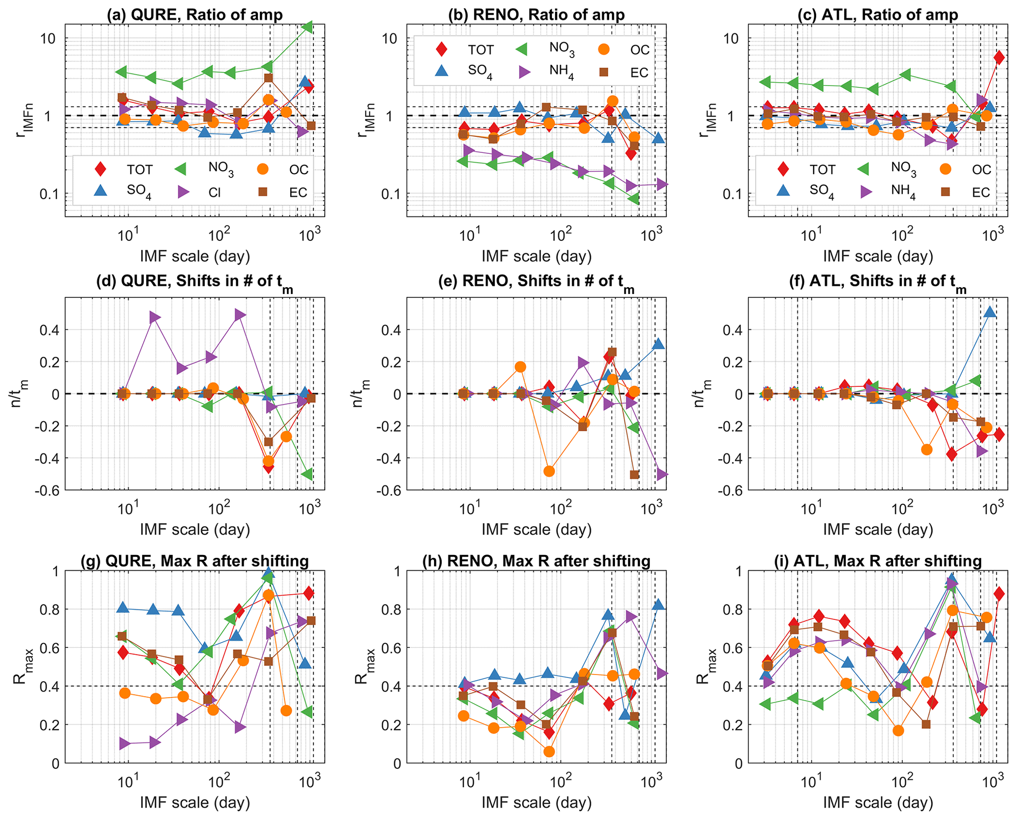
Figure 11 Model performance at all temporal scales for sites QURE, RENO, and ATL. (a–c) Ratio of mean amplitude of corresponding IMFs with similar characteristic mean periods (ideal ratio = 1.0); (d–f) the phase shift n in the number of mean periods (average mean period of corresponding IMFs decomposed from observations and model simulation). (g–i) The maximum correlation R_max can be achieved by shifting the modeled time series. The average mean period of corresponding IMFs decomposed from observations and CMAQ of total and speciated PM_2.5 are represented on the x axis; all metrics on the y axis are unitless. Horizontal reference lines are drawn at 0.7 and 1.3 in (a–c). Weekly, annual, and interannual (2- to 3-year) scales are marked with dashed vertical lines.

The performance of the simulated amplitude of the sub-seasonal and interannual cycles is relatively stable from a few days to semi-annual scales, and r_IMFn is close to 1 in most cases (Fig. 11a–c). CMAQ captures the features seen in the observations at QURE, except for the large overestimation of NO₃ (r_IMFn ranges from 2.6 to 3.7 at the sub-seasonal scale and reaches up to 13.8 for the 3-year cycles). Similar overestimation of NO₃ is also found at ATL (r_IMFn ranges from 2.0 to 3.4, except for the 2-year cycles). In contrast, NO₃ at RENO is strongly underestimated, with r_IMFn ranging from 0.1 to 0.3 and reaching its minimum in the 2-year cycles. Likewise, all timescales of NH₄ at RENO are also being underestimated, with r_IMFn decreasing from 0.4 to only 0.1 in the 3-year cycles. The coexistence of underestimation of NO₃ and NH₄ variability, as well as their trend component, likely points to the insufficient grid resolution in representing ammonium nitrate episodes associated with stagnant meteorology in the mountainous regions as illustrated by Kelly et al. (2019). To sum up, the model has simulated the magnitude of features across all scales in most of the studied cases. However, fluctuations in NO₃ are constantly being largely over- or underestimated, and improvements to the model are required to better replicate its variability (Fig. 11a–c).

A high R_max of corresponding IMFs can only be achieved when the characteristic scales of those from observations and model simulations are close, there is minimal mode mixing, and negligible irregular change of amplitude exists during the study period. Thus, R_max tends to be small for all oscillations at RENO because of the irregular impact from events such as wildfires. Thus, the interpretation of phase shift is focused on the components and timescales with correlations above 0.4 only.

Results show that the sub-seasonal cycles at QURE all have a negligible phase shift of less than 0.1 cycles (Fig. 11d). The semi-annual cycles at RENO have around 0.2 cycle phase shifts in total PM_2.5 (−0.2), NH₄ (0.2), OC (−0.2), and EC (−0.2), while negligible phase shifts of less than 0.1 cycles are simulated in SO₄ ranging from 9 d to being semi-annual in scale. As at QURE, multiple sub-seasonal cycles at ATL all have a negligible phase shift of less than 0.1 cycles, with the exception of semi-annual OC which has a phase shift of nearly −0.4 cycles, with a marginal correlation of around 0.4. Unlike the relatively stable R_max throughout the timescales within each of the species for QURE and RENO, the R_max at ATL tends to be much higher (roughly 0.6–0.8) in the scales of 6 to 25 d, except for NO₃, indicating the model's success in simulating the weather-induced air quality fluctuations at this site as reflected by their negligible phase shifts.

However, the physical meaning of each sub-seasonal IMF is not yet fully understood and requires further study. For example, synoptic-scale IMFs (IMFs with scales less than/around a month) usually have large variance and are not statistically significantly different from white noise except for observed SO₄ and NH₄ (Fig. S5). Yet, observed and simulated total and some speciated PM_2.5 at QURE and ATL (except IMF1) can achieve moderate to high R_max at these timescales (Fig. 11g–i), indicating a potential physical explanation for those timescales using meteorological variables. IMFs with scales longer than a month but less than half a year possess much less variance and are usually not statistically significantly different from noise. Exceptions are also found at the Atlanta site, where observed IMFs are mostly significantly different from noise, whereas semi-annual cycles are mostly statistically significant (note that semi-annual SO₄ and NO₃ at ATL are too weak to be decomposed into a separate IMF). In a previous study, He et al. (2014) found semi-annual oscillations in the corrected AErosol RObotic NETwork (AERONET) aerosol optical depth (AOD) and that PM₁₀ mass concentrations are primarily caused by the change of wind direction in Hong Kong.

The evaluation and interpretation of interannual cycles are constrained by the limited available speciated observations for a period of 6 to 9 years (4 years for Cl at QURE). Thus, only 2- to 3-year cycles are presented (Fig. 11) and evaluated. Among the 2- to 3-year interannual cycles at QURE, there is minimal phase shift for total PM_2.5, SO₄, Cl, and EC, with moderate to high R_max. At RENO, the model presents negligible shifts in 2-year cycles of OC and NH₄, while phase shifts of 0.3 and −0.5 cycles are simulated in the 3-year cycles for SO₄ and NH₄. At ATL, the phase shift of −0.2 to −0.4 cycles is simulated for PM_2.5, NH₄, OC, and EC with periods of 2- to 3-year cycles, while 2- to 3-year SO₄ cycles have a half-year cycle shift.

5 Conclusions

The main advantage of using EMD to evaluate PM_2.5 and its speciated components is that it decomposes nonlinear and nonstationary signals into multiple modes and a residual trend component. It does not require any preselection of the temporal scales and assumptions of linearity and stationarity for the data, thereby providing insights into time series of PM_2.5 concentrations and its components. Using improved CEEMDAN, we are able to assess how well regional-scale air quality models like CMAQ can simulate the intrinsic time-dependent long-term trend and cyclic variations in daily average PM_2.5 and its species. This type of coordinated decomposition and evaluation of total and speciated PM_2.5 provides a unique opportunity for modelers to assess influences of each PM_2.5 species to the total PM_2.5 concentration in terms of time shifts for various temporal cycles and the magnitude of each component including the trend.

A demonstration of how improved CEEMDAN could be applied to PM_2.5 time series at three sites over CONUS that provide speciated PM_2.5 data reveals the presence of the annual cycles in PM_2.5 concentrations and time-dependent features in all decomposed components. At these three sites, the model generally is more capable of simulating the change rate in the trend component than the absolute magnitude of the long-term trend component. However, the magnitude of SO₄ trend components is well represented across all three sites. Also, the model reproduced the amplitude of the annual cycles for total PM_2.5, SO₄, and OC. The phase difference in the annual cycles for total PM_2.5, OC, and EC reveals a shift of up to half a year, indicating the need for proper allocation of emissions and an updated treatment of organic aerosols compared to the earlier model version used in this set of model simulations. The consistent large under-/overprediction of NO₃ variability at all temporal scales and magnitude in the trend component, as well as the abnormally low correlations of synoptic-scale NO₃ at ATL, calls for better representation of nitrate partitioning and chemistry. Wildfires have the potential to elevate PM_2.5 for months and can alter its variability at scales from a few days to an entire year. Thus, more accurate fire emission data should be incorporated to improve model simulation, especially in these fire-prone regions.