Investigation of the wet removal rate of black carbon in East Asia: validation of a below- and in-cloud wet removal scheme in FLEXible PARTicle (FLEXPART) model v10.4

Understanding the global distribution of atmospheric black carbon (BC) is essential for unveiling its climatic effect. However, there are still large uncertainties regarding the simulation of BC transport due to inadequate information about the removal process. We accessed the wet removal rate of BC in East Asia based on long-term measurements over the 2010–2016 period at three representative background sites (Baengnyeong and Gosan in South Korea and Noto in Japan). The average wet removal rate, represented by transport efficiency (TE), i.e., the fraction of undeposited BC particles during transport, was estimated to be 0.73 in East Asia from 2010 to 2016. According to the relationship between accumulated precipitation along trajectory and TE, the wet removal efficiency was lower in East and North China but higher in South Korea and Japan, implying the importance of the aging process and frequency of exposure to below- and in-cloud scavenging conditions during air mass transport. Moreover, the wet scavenging in winter and summer showed the highest and lowest efficiency, respectively, although the lowest removal efficiency in summer was primarily associated with a reduced BC aging process because the in-cloud scavenging condition was dominant. The average half-life and e-folding lifetime of BC were 2.8 and 7.1 d, respectively, which is similar to previous studies, but those values differed according to the geographical location and meteorological conditions of each site. Next, by comparing TE from the FLEXible PARTicle (FLEXPART) Lagrangian transport model (version 10.4), we diagnosed the scavenging coefficients (s⁻¹) of the below- and in-cloud scavenging scheme implemented in FLEXPART. The overall median TE from FLEXPART (0.91) was overestimated compared to the measured value, implying the underestimation of wet scavenging coefficients in the model simulation. The median of the measured below-cloud scavenging coefficient showed a lower value than that calculated according to FLEXPART scheme by a factor of 1.7. On the other hand, the overall median of the calculated in-cloud scavenging coefficients from the FLEXPART scheme was highly underestimated by 1 order of magnitude, compared to the measured value. From an analysis of artificial neural networks, the convective available potential energy, which is well known as an indicator of vertical instability, should be considered in the in-cloud scavenging process to improve the representative regional difference in BC wet scavenging over East Asia. For the first time, this study suggests an effective and straightforward evaluation method for wet scavenging schemes (both below and in cloud), by introducing TE along with excluding effects from the inaccurate emission inventories.

1 Introduction

Black carbon (BC) is the most significant light-absorbing aerosol that can cause positive radiative forcing on climate change (Winiger et al., 2016; Myhre et al., 2013; Bond et al., 2013; Emerson et al., 2018). However, state-of-the-art models still have limitations in evaluating the direct radiative forcing of BC because of the large model uncertainties in simulating BC concentrations (Xu et al., 2019; Bond et al., 2013; Samset et al., 2014; Q. Wang et al., 2014; Schwarz et al., 2010; Sharma et al., 2013). This can partly be attributed to the following three reasons: (1) inaccurate bottom-up emission inventory, (2) the complexity of BC hygroscopicity, and (3) an imprecise dry and/or wet deposition scheme. First, when estimating the impact of BC using global models, the results usually contain large uncertainties in BC emissions (Cooke and Wilson, 1996; Chung and Seinfeld, 2002; Stier et al., 2007) because BC is mainly emitted by scattered emission sources. Therefore, the uncertainty of BC emission rates is large compared to other species (e.g., SO₂, NO_x, and CO₂) whose emissions are dominated by large sources (Kurokawa et al., 2013; Zheng et al., 2018). Without appropriate constraints on the emissions, removal cannot be well quantified. Second, although BC itself is hydrophobic immediately after emission, it is subsequently converted to a substance possessing hydrophilic properties, through the aging process, in which water-soluble compounds coat BC during atmospheric transportation (Moteki et al., 2007; Matsui et al., 2018) and, finally, act as cloud condensation nuclei (Kuwata et al., 2007; Bond et al., 2013). Such a conversion depends on the initial state of the BC along with atmospheric conditions (presence of other particles and gases), and it has high spatial and temporal variabilities (Vignati et al., 2010). Third, while BC particles are transported in the atmosphere, they can be removed by dry and/or wet deposition, including below-cloud (i.e., washout) and in-cloud (i.e., rain out.) processes. Wet deposition of BC, whose contribution to total removal is 79 % (Textor et al., 2006), is still challenging for predicting BC concentrations in the atmosphere due to the difficulties of accurate evaluation of wet removal (Emerson et al., 2018; Bond et al., 2013; Lee et al., 2013). Specifically, the in-cloud process is more efficient and complicated than the below-cloud process because the nucleation removal of aerosol particles within clouds is thought to account for 46 %±50 % of BC particle mass removal from the atmosphere globally, although this is dependent on the selected global model (Grythe et al., 2017; Textor et al., 2006). However, there is insufficient in-field detailed observations to explain and quantify the interactions between BC and cloud particles at the microscale, which hinders a better understanding of the physical processes (Ding et al., 2019).

Accompanied with the refinement of BC emission inventories over East Asia (Choi et al., 2020; Kanaya et al., 2016), wet removal rates have been a focal point for better a prediction of BC behavior by using the term transport efficiency (TE), which is the observationally determined fraction of undeposited BC particles during transport (e.g., Oshima et al., 2012; Kondo et al., 2016) because TE shows a good relationship with the accumulated precipitation along trajectory (APT; sum of precipitation over the past 72 h backward trajectory; Choi et al., 2020; Kanaya et al., 2016). Moteki et al. (2012), who were further elaborated on by Oshima et al. (2012), reported the first observational evidence of the size-dependent activation of BC removal over the Yellow Sea during the Aerosol Radiative Forcing in East Asia (A-FORCE) airborne measurement campaign in the spring of 2009. Kondo et al. (2016) demonstrated an altitude dependence, with typical decreasing size distributions at higher altitudes, associated with wet removal from A-FORCE in winter 2013. Kanaya et al. (2016) elucidated the relationship between the wet removal rate of BC and APT from long-term measurements (2009–2015) at Fukue, Japan. Miyakawa et al. (2017) reported the effects of BC aging related to in-cloud scavenging during transport on the alteration of the BC size distribution and mixing states during the spring of 2015 at the same location. Matsui et al. (2013) demonstrated that the difference in the coating thickness of BC particles depended on the growing process (condensation and coagulation), indicating that the coagulation process is necessary to produce thickly coated BC particles that are preferentially removed via the wet scavenging process. Recently, numerous fine mode particles, including BC, from polluted areas scavenging in clouds were more pronounced in East Asia, not only at a local scale but also at a large regional scale (Liu et al., 2018), because high aerosol loading conditions are usually associated with considerable cloud cover, which results in a higher frequency of wet scavenging (Eck et al., 2018).

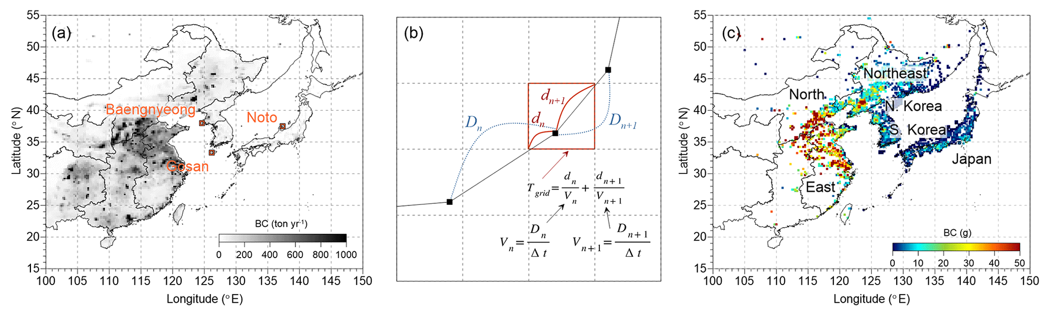
Figure 1 (a) The location of the three measurement sites (Baengnyeong, Gosan, and Noto) and the black carbon (BC) emission rate (t yr⁻¹) over East Asia from the Regional Emission inventory in ASia (REAS) version 2.1 (Kurokawa et al., 2013). (b) Illustration of residence time calculated based on the HYSPLIT backward trajectory that passed over a single grid cell (see details in the text). (c) The location of administrative districts, and the spatial distribution of the mean BC mass in the potential emission region, which is the highest BC mass grid of each trajectory. The BC mass was obtained by multiplying (a) the emission rates and (b) the residence time.

BC and carbon monoxide (CO) are byproducts of the incomplete combustion of carbon-based fuels, and the ratio between ΔBC (the difference from the baseline level) and ΔCO is a useful parameter for characterizing fuel types because of their different carbon contents (Zhou et al., 2009; Guo et al., 2017). Adopting APT, a useful index for the strength of wet deposition (Kanaya et al., 2016, 2020), the magnitude of the BC wet removal rate can be easily characterized by the relationship between TE and APT. Although some previous studies have investigated wet scavenging schemes in models (Grythe et al., 2017; Croft et al., 2010), those results without well-constrained emission rates contain large ambiguity when assessing the wet deposition term (Vignati et al., 2010). For the first time, the emission and deposition terms are distinctly separated in this study by introducing TE and using backward simulations, thus allowing for the wet scavenging scheme to be evaluated more accurately because backward simulations do not account for the emission rate. By elaborating on the regional ΔBC∕ΔCO ratio (Choi et al., 2020), this study investigates the characteristics of the BC wet removal rate over East Asia using long-term measurements (more than 3 years) to acquire reliable BC concentrations with a wide spatial coverage over East Asia. The differences in the wet removal rates, depending on the measurement sites and six administrative districts (Fig. 1c) and season, are discussed in Sect. 3.1 and 3.2, respectively. Afterwards, to evaluate the representativeness of the scavenging scheme in the recently updated FLEXible PARTicle dispersion model (FLEXPART) version 10.4, the wet scavenging coefficients for below- and in-cloud processing were validated with the measured wet removal rate by allocating the air mass location (such as below or within clouds) and meteorological variables along the pathway of air mass transport.

2 Methods

2.1 Measurement sites and instruments

To investigate the wet removal rates of the outflow air mass from China and the Korean peninsula, BC and CO data from three measurement sites (Baengnyeong and Gosan in Korea and Noto in Japan; Fig. 1a) were carefully selected for this study by considering major emission sources near the measurement sites and by obtaining reliable BC concentrations from different instruments. Because detailed information on the measurement sites and instruments is described in Choi et al. (2020), we only address this information briefly here. Baengnyeong (124.63^∘ E, 37.97^∘ N), one of the intensive measurement stations operated by the Korean Ministry of Environment, is frequently affected by air masses from China (including East, North, and Northeast China) and North Korea. Gosan (126.17^∘ E, 33.28^∘ N) is located in the southern part of Korea and is frequently affected by air masses from East China and South Korea. BC and CO were also measured at the Noto Ground-based Research Observatory (NOTOGRO; 137.36^∘ E, 37.45^∘ N), located on the Noto Peninsula on the western coast of Japan, which is frequently affected by air masses from Northeast China and Japan. The measurement periods were mainly in the early 2010s but were slightly different depending on the sites (Fig. S1 in the Supplement). The longest measurement period was in Noto for approximately 6 years (from 2011 to 2016), followed by that in Baengnyeong (5 years; 2010 to 2017, excluding 2011 to 2012) and Gosan (3 years; 2012 to 2015).

In this study, we tried to obtain reliable BC concentrations from well-validated instruments, including organic carbon and elemental carbon (OC–EC) analyzers (Sunset Laboratory Inc., USA) with optical corrections, multi-angle absorption photometers (MAAPs; MAAP 5012; Thermo Scientific, USA), and a continuous light absorption photometer (CLAP), that yielded good agreements in the BC concentrations between the instruments (uncertainty $\le \pm \mathrm{15}$ %, except for CLAP at $\le \pm \mathrm{20}$ %; Choi et al., 2020; Kanaya et al., 2008, 2013; Miyakawa et al., 2016, 2017; Taketani et al., 2016). Hourly PM_2.5 elemental carbon (EC) was measured by an OC–EC analyzer for Baengnyeong. A MAAP was used to measure hourly BC in PM_2.5 at Noto. At Gosan, BC in PM₁ was monitored by a CLAP with three wavelengths, including 467, 528, and 652 nm, and the absorption was corrected following Bond et al. (1999). For MAAP, an improved mass absorption efficiency (MAE) of 10.3 m² g⁻¹ (instead of the default value of 6.6 m² g⁻¹) was applied to estimate the BC mass concentration as suggested, based on calibrations using the thermal∕optical method and the laser-induced incandescence technique (Kanaya et al., 2013, 2016). The CLAP also showed a good correlation with the colocated PM_2.5 EC concentrations from the OC–EC analyzer, and the best-fit line was close to one (1.17), which is similar to or slightly lower than the range of reported uncertainty of ∼25 % (Ogren et al., 2017). Hourly CO concentrations were measured by a gas filter correlation CO analyzer (Model T300; Teledyne Technologies Incorporated) at Baengnyeong and by a nondispersive infrared absorption photometer (48C; Thermo Scientific, USA) at the other two sites. The overall uncertainty of the CO measurements from different instruments was estimated to be less than 5 %, which led to a 10 % uncertainty in the overall regional ΔBC∕ΔCO ratio (Choi et al., 2020).

2.2 Backward trajectory and meteorological data

To identify the source region of air mass, 5 d (120 h) backward trajectories were calculated four times a day (00:00, 06:00, 12:00, and 18:00 coordinated universal time – UTC) using the Hybrid Single Particle Lagrangian Integrated Trajectory (HYSPLIT) model version 4 (Draxler et al., 2018). The starting altitude was 500 m abovegroundlevel (a.g.l.). The past 120 h of backward simulation time was selected by considering the lifetime of BC (∼5 d; Lund et al., 2017, 2018; Park et al., 2005). It should be noted that the different starting altitude (500 m vs. 1000 m) did not impact on our results (Sect. S1 in the Supplement). Notably, we used the European Centre for Medium-Range Weather Forecasts (ECMWF) ERA5, which provides a much finer resolution of $\mathrm{0.25}{}^{\circ }\times \mathrm{0.25}{}^{\circ }$, as input for HYSPLIT instead of the Global Data Assimilation System (GDAS; $\mathrm{1}{}^{\circ }\times \mathrm{1}{}^{\circ }$), to improve the accurate assessment of the air mass transportation pathways and to acquire more detailed information on the meteorological conditions. According to the pathway of air mass transportation, the detailed meteorological information, such as precipitation (sum of the large-scale and convective precipitation), clouds, and so on, was acquired from ERA5 hourly data at both single and pressure levels (37 levels; 1000 to 1 hPa). By considering the vertical height of the air mass from the HYSPLIT model and cloud information from ERA5, we successfully distinguished the dominant cases for below-cloud (no residence time within the cloud) and in-cloud (no residence time below the cloud) cases when precipitation ≥0.01 mm h⁻¹, and calculated the wet scavenging coefficients.

As the air mass was being transported, if precipitation occurred before the air mass arrived at the main BC source region, which is the highest BC emission area, then the magnitude of the wet removal effect as a function of APT could be underestimated at receptor sites because the air mass containing BC would not have been exposed to wet scavenging conditions. Therefore, we considered the residence time (Li et al., 2014; Ashbaugh et al., 1985) of each grid cell ($\mathrm{0.25}{}^{\circ }\times \mathrm{0.25}{}^{\circ }$) and the BC emission rates (mass time⁻¹) from the Regional Emission inventory in ASia (REAS; Fig. 1a) emission inventory (Kurokawa et al., 2013) version 2.1 to identify the potential emission region by multiplying the residence time and emission rates. First, when the air mass altitude was lower than 2.5 km, the air mass velocities (V_n and V_n+1) were calculated as distances from the central point in a target grid cell to two-way endpoints of backward trajectories (D_n and D_n+1) using $V_n=D_n/\mathrm{\Delta }t$ and $V_{n+\mathrm{1}}=D_{n+\mathrm{1}}/\mathrm{\Delta }t$ (Fig. 1b), where Δt and n represent the time interval of the meteorological data (1 h) and nth grid cell, respectively. Then, by assuming that the air mass velocity is constant within the time interval, the residence time in a grid cell (T_grid) was calculated by considering both the distance of each grid corner (d_n and d_n+1) and the corresponding velocities (V_n and V_n+1) using $d_n/V_n+d_{n+\mathrm{1}}/V_{n+\mathrm{1}}$. Based on the identified potential emission region, APT was recalculated only after the air mass passed through the potential emission region when APT over the past 72 h was higher than 0. Figure 1c reveals the geographical distribution for the mean BC mass of identified potential emission regions, indicating that this approach was appropriate because the potential emission regions were uniformly distributed over East Asia, including East China, a major emission source for BC. We checked the uncertainty arising from selecting different criteria for altitude (1.5 km), but there was no significant difference in the results (Sect. S1 in the Supplement).

2.3 Transport efficiency (TE)

The TE of BC is defined as the ratio of the BC and CO concentrations measured at the receptor site to that anticipated if there was no wet removal during transport (i.e., APT during past 72 h is zero). Thus, the TE of the air mass was calculated by Eq. (1) as follows:

$$\begin{array}{}\text{(1)}& {\displaystyle }\text{TE}={\displaystyle \frac{{\left[\mathrm{\Delta }\text{BC}/\mathrm{\Delta }\text{CO}\right]}_{\text{APT}>\mathrm{0}}}{{\left[\mathrm{\Delta }\text{BC}/\mathrm{\Delta }\text{CO}\right]}_{\text{APT}=\mathrm{0}}}},\end{array}$$

where delta (Δ) indicates the difference between BC and CO concentrations and their baseline concentrations (Moteki et al., 2012; Oshima et al., 2012; Kanaya et al., 2016). The baseline CO was estimated as being a 14 d moving fifth percentile from the observed CO mixing ratio, but the BC baseline was regarded as being zero because the atmospheric lifetime of BC is known to be several days, which is much shorter than that of CO (1–2 months). [ΔBC∕ΔCO]_APT=0 indicated the regional median value of ΔBC∕ΔCO under dry conditions, implying the original emission ratio. In our previous work, we successfully elucidated that [ΔBC∕ΔCO]_APT=0 depends on the regional characteristics of the energy consumption types (Kanaya et al., 2016; Choi et al., 2020). The decrease in the ratio with APT, [ΔBC∕ΔCO]_APT>0, was related to BC-specific removal due to wet scavenging processes, and thus, the TE is an effective indicator for the investigation of the wet removal process. Although TE is also affected by dry deposition, Choi et al. (2020) reported that the effect of dry deposition could be neglected because dry deposition velocities (0.01–0.03 cm s⁻¹) are much lower than the default setting (0.1 cm s⁻¹) in global models (Chung and Seinfeld, 2002; Cooke and Wilson, 1996; Emmons et al., 2010; Sharma et al., 2013).

2.4 FLEXPART model

To compare the TE between the measured values and model simulation, the FLEXPART v10.4 was used to simulate BC wet scavenging over East Asia using the backward mode. Detailed information on the FLEXPART is readily found in the literature (e.g., Pisso et al., 2019, and Stohl et al., 2005); thus, we only briefly describe the information here. The FLEXPART version 10.4 is the official version that allows for the turning on of the wet scavenging module in the backward simulation mode (https://www.flexpart.eu/downloads, last access: 10 October 2019). The equations and detailed descriptions of the below- and in-cloud scavenging scheme are explained in Pisso et al. (2019) and Grythe et al. (2017). The FLEXPART model was executed with reanalysis meteorological data from the ECMWF ERA-Interim at a spatial resolution of $\mathrm{1}{}^{\circ }\times \mathrm{1}{}^{\circ }$ with 60 model levels from the surface up to 0.1 hPa. Temporally, ERA-Interim has a resolution of 3 h, with a 12 h analysis and 3 h forecast time steps. The period and daily frequency of the simulation were the same as those of the HYSPLIT model (the past 72 h and four times, respectively). The grid resolution of FLEXPART was also the same with ECMWF ERA-Interim ($\mathrm{1}{}^{\circ }\times \mathrm{1}{}^{\circ }$). It should be noted that chemistry and microphysics could not be resolved by the FLEXPART. The FLEXPART model, therefore, ignores the aging process (from hydrophobic to hydrophilic state changes and size changes in BC) and assumes that all BC particles are aged hydrophilic particles. A logarithmic size distribution of BC, with a mean diameter of 0.16 µm and a standard deviation of 1.84 in accordance with measurement in Japan, was used (Miyakawa et al., 2017). A total of 10⁴ particles were randomly released at 500 m from each receptor site during 1 h when the measurement data were available. To validate the wet scavenging scheme in FLEXPART by comparison with the measured TE value, the wet scavenging coefficients for below and in clouds were extracted from FLEXPART to calculate TE (see Sect. 3.3 for more details). Note that the simulated TE from FLEXPART (FLEXPART TE) was only used for a comparison with the measured TE. Despite the difference in the meteorological input fields between HYSPLIT and FLEXPART, the difference in air mass pathways and APT between two data sets can be neglected (Hoffmann et al., 2019; Sect. S2 in the Supplement).

3 Results

3.1 Overall variation of transport efficiency (TE)

Figure 2 shows that measured [ΔBC∕ΔCO]_APT=0 (left panel) and TE variations (right panel) depend on APT and the measurement sites. The overall median [ΔBC∕ΔCO]_APT=0 was 6.4 $\mathrm{ng}{\mathrm{m}}^{-\mathrm{3}}{\mathrm{ppb}}^{-\mathrm{1}}$, which converged from Baengnyeong (6.2 $\mathrm{ng}{\mathrm{m}}^{-\mathrm{3}}{\mathrm{ppb}}^{-\mathrm{1}}$), Gosan (6.5 $\mathrm{ng}{\mathrm{m}}^{-\mathrm{3}}{\mathrm{ppb}}^{-\mathrm{1}}$), and Noto (6.7 $\mathrm{ng}{\mathrm{m}}^{-\mathrm{3}}{\mathrm{ppb}}^{-\mathrm{1}}$), indicating that TE is characterized by a regional [ΔBC∕ΔCO]_APT=0 per site. We divided APT into nine range bins and applied exponential fitting equations to quantify the wet removal process. Among N_APT>0 (total number of data points when APT>0 mm), only the data point fraction in each bin to $N_{\text{APT}>\mathrm{0}}\ge \mathrm{2}$ % was considered to secure the statistic. It should be noted that we found the relationship between TE and APT by using the stretched exponential decay (SED) equation, $\exp (-A_{\mathrm{1}}\times {\text{APT}}^{A_{\mathrm{2}}}$), instead of the widely used equation, $A-B\times \log (\text{APT}$), because the coefficient of determination (R²) was improved from 0.940 to 0.981 though TE values from three sites were used (Table 1). This fitting equation is normally used to describe below-cloud scavenging, whereas wet removal of BC is generally believed to be dominated by in-cloud rather than below-cloud processes because of the small size of the BC-containing particles. Therefore, the equations should contain both below- and in-cloud scavenging effects. The parameters A₁ (0.269±0.039) and A₂ (0.385±0.035) of the overall fitting were higher and lower, respectively, than the derived equation from the Fukue site (A₁=0.109 and A₂=0.68), which is the remote site in Japan (128.68^∘ E, 32.75^∘ N; Kanaya et al., 2016). It can be easily deduced that the wet removal effect at the three sites was initially more effective than that at Fukue, but the wet removal effect at Fukue gradually accelerated as the APT increased. In particular, the A₂ value is important for calculating the amount of BC from emission sources via long-range transport, e.g., toward the Arctic (Kanaya et al., 2016; Zhu et al., 2020), because A₂ determines the magnitude of the wet removal efficiency according to APT. Thus, the newly obtained SED equation, which has a low A₂ value, indicates that more BC might be transported to the Arctic region than that reported by Kanaya et al. (2016).

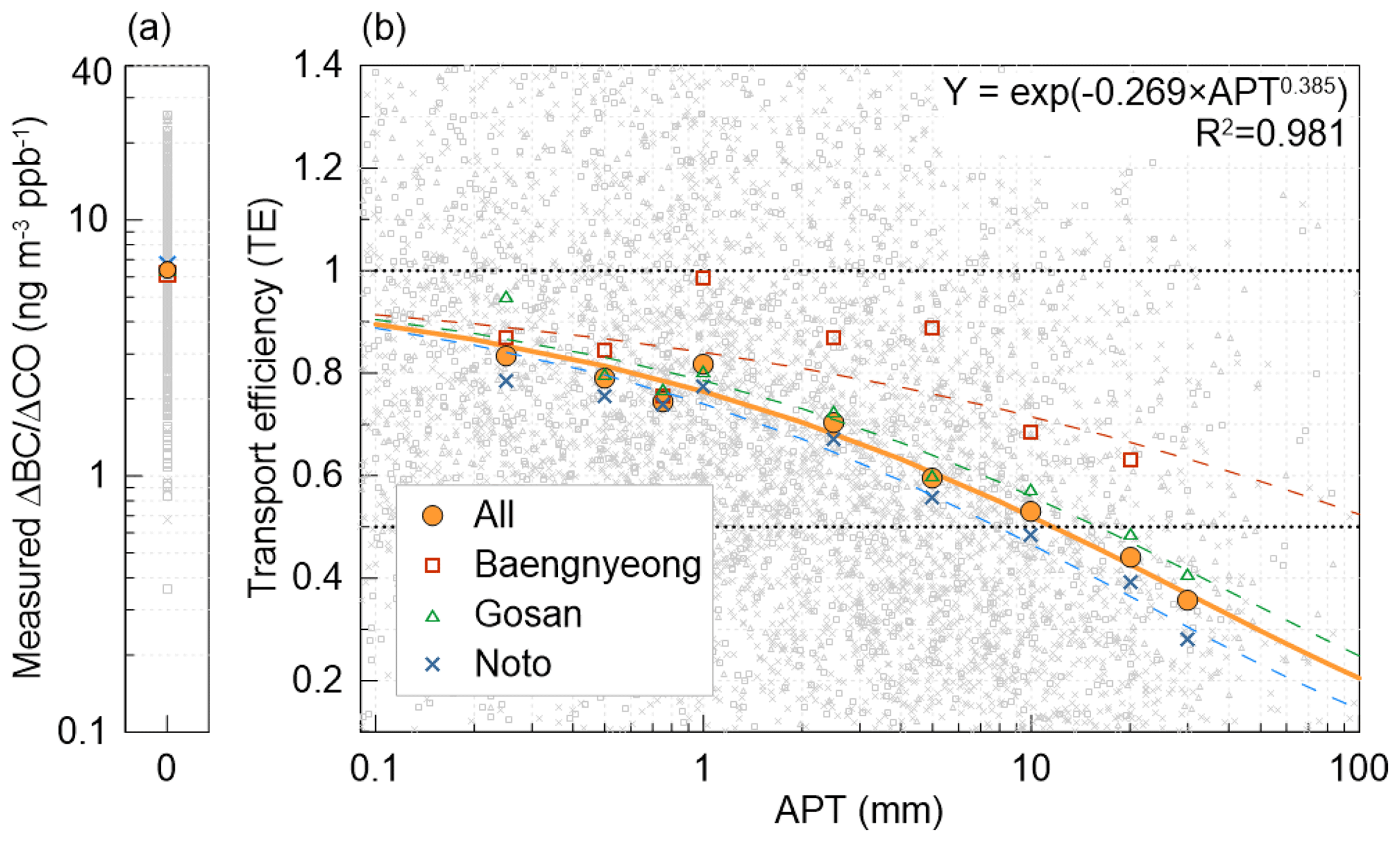
Figure 2 Measured ΔBC∕ΔCO ratios, when accumulated precipitation along trajectory (APT) was zero (a) and transport efficiency (TE) variation was a function of APT (b), depending on the different sites and overall cases. All data (gray with different symbols) and nine bins sorted by APT (different colored symbols) are shown. The horizontal dotted lines indicate TE at 0.5 and 1, respectively. The nine bins consist of 0.01–0.25, 0.25–0.50, 0.50–0.75, 0.75–1.0, 1.0–2.5, 2.5–5.0, 5.0–10, 10–20, and 20–30 mm.

Table 1 Summary of the relationship between transport efficiency (TE) and accumulated precipitation along trajectory (APT) in Figs. 2 and 4.

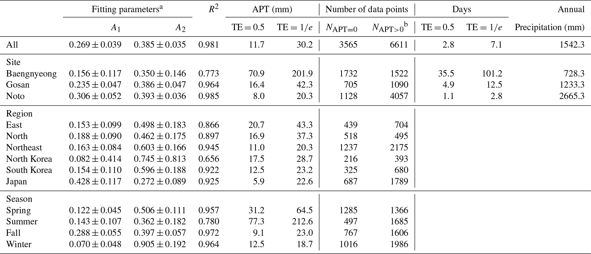
^a $\text{TE}=\exp (-A_{\mathrm{1}}\times {\mathrm{APT}}^{A_{\mathrm{2}}})$. ^b The number of satisfactory data points in each bin relative to total $N_{\text{APT}>\mathrm{0}}\ge \mathrm{2}$ %.

The decreasing pattern of median TE for Baengnyeong did not closely follow the overall SED and had a much lower R² (0.77), indicating that the wet removal process at Baengnyeong could not simply be expressed by APT. In contrast, the R² of Gosan and Noto were sufficiently high enough to represent the wet removal characteristics. The aging process due to different traveling times might be one of the reasons. Because long-range transported BC has a larger core diameter than BC from local sources (Lamb et al., 2018; Ueda et al., 2016), these larger BC cores are preferentially removed via the wet scavenging process (Moteki et al., 2012). Previous studies reported that the mass median diameter (MMD) of refractory BC (rBC) at Baengnyeong, Gosan, and Noto in spring was 218, 196, and 200 nm, respectively (Oh et al., 2014, 2015; Ueda et al., 2016), indicating much more aging compared with local emissions in Seoul, South Korea (180 nm), and Tokyo, Japan (163 nm; Park et al., 2019; Ohata et al., 2019). In addition, the difference in the wet removal rate depending on measurement sites could be partly explained by differences in meteorology. The monthly mean meteorological parameters indicated that Baengnyeong has characteristics of low precipitation (80.6 mm), cloud cover (0.57), total column cloud water (0.06 kg m⁻²), and high cloud bottom height (2.5 km) compared to other sites, suggesting a lower exposure time to both below- and/or in-cloud conditions during transportation (Fig. 3). In contrast, both Gosan and Noto showed similar ranges of high precipitation (127 and 174 mm), total cloud cover (0.65 and 0.64), and total column cloud water (0.09 and 0.12 kg m⁻²) but low cloud bottom height (1.9 and 2.0 km), respectively. In addition, the difference in magnitude of aging BC and frequency of exposure to below- and in-could scavenging conditions will be further discussed in Sect. 3.2.

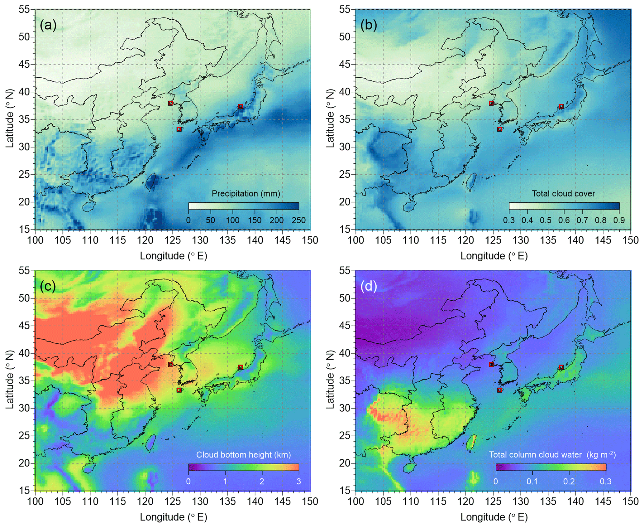
Figure 3 Monthly mean meteorological fields over East Asia from 2010 to 2016 derived from the European Centre for Medium-Range Weather Forecasts (ECMWF) ERA5 monthly averaged data at single levels. (a) Precipitation (millimeters), (b) total cloud cover, (c) cloud bottom height (kilometers), and (d) total column cloud total water (ice and liquid).

Using the overall SED fitting equation, TE at 0.5 (TE = 0.5) and e folding ($\text{TE}=\mathrm{1}/e$) could be reached when the APT values were 11.7 and 30.2 mm, respectively (Table 1). Similar to the SED results, Baengnyeong needed much higher precipitation of 70.9 and 202 mm to reach TE = 0.5 and $\text{TE}=\mathrm{1}/e$, respectively, but the other sites showed lower APTs of 16.4 and 42.3 mm for Gosan and 8.0 and 20.3 mm for Noto, respectively. Considering the annual mean precipitation at the three sites (1542 mm), it took 2.8 and 7.1 d to reach TE = 0.5 and $\text{TE}=\mathrm{1}/e$, respectively. Kanaya et al. (2016) reported a similar half-life and shorter e-folding lifetime for BC at Fukue (2.3±1.0 and 4.0±1.0 d, respectively), calculated from the 15.0±3.2 mm and 25.5±6.1 mm of APT to reach TE = 0.5 and $\text{TE}=\mathrm{1}/e$, respectively, along with annual precipitation of 2335 mm. This calculated e-folding lifetime in East Asia was much shorter than 16.0 d for BC from FLEXPART v10 (Grythe et al., 2017).

Based on a similar approach over the Yellow Sea using an aircraft-borne single particle soot photometer (SP2) during the A-FORCE campaign (Oshima et al., 2012), attaining TE = 0.5 required different magnitudes of APT depending not only on the air mass origin but also on the altitude. These authors also reported that the TE of northern China was higher than that of southern China regardless of altitude. Therefore, in the next section, we will further investigate why the difference in halving or e-folding lifetimes depends on region and season by analyzing the differences in the pathway of air masses.

3.2 Regional and seasonal variations of the transport efficiency (TE)

Figure 4 indicates the variation in TE depending on the potential source regions (hereafter regions) and seasons. The R² for each region varied from 0.656 to 0.945 and was lower in East and North China and North Korea and higher in other regions (Table 1). Similar to the tendency of R², the APTs for achieving TE = 0.5 also showed regional differences, i.e., higher in East and North China and lower in other regions. The regional differences in wet removal efficiency can partly be attributed to the following reasons.

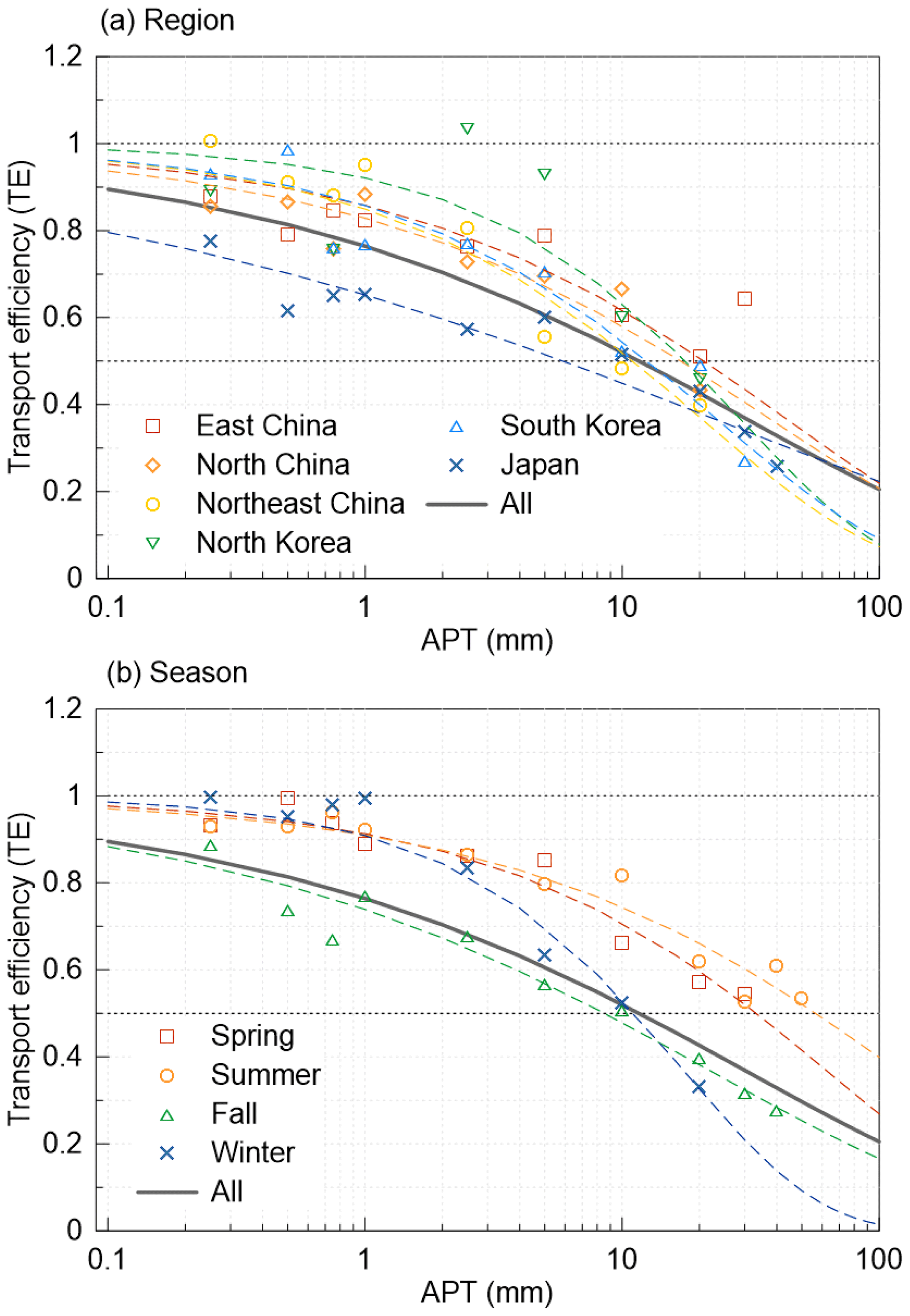
Figure 4 Same as Fig. 2 except for (a) regional and (b) seasonal variations in TE according to APT. Each colored symbol and dashed line indicates the different regions and seasons and fitting lines according to stretched exponential decay (SED). The thick gray line depicts the overall fitting line. The horizontal dotted lines indicate TE at 0.5 and 1, respectively.

First, the transport pathway of air masses from East and North China could be less exposed to in-cloud scavenging than other regions because most of the potential emission sources in East and North China are located over 30^∘ N (Fig. 1c), which has low cloud cover and water content along with high cloud bottom heights (Fig. 3). Although the amount of APT was similar to that in other regions, it was mostly composed of below-cloud scavenging; therefore, the wet removal efficiency should be lower than that in the dominant in-cloud scavenging region. To quantify the effect of below- and in-cloud scavenging, we investigated the fraction of exposure to below- and in-cloud scavenging conditions during the air mass transport according to regions. Among the total frequency of grid cells which air masses passed (∼ 500 000), ∼25 % of the grid cells were exposed to below- (∼10 %) and in-cloud scavenging conditions (∼15 %), indicating that the in-cloud conditions were relatively predominant in wet scavenging over East Asia. The higher wet removal efficiency region (South Korea and Japan) revealed an apparently higher fraction of exposure to below- (∼11 %) and in-cloud scavenging conditions (∼19 %) compared to the air masses from East and North China (∼8 % for below- and ∼10 % for in-cloud scavenging conditions), suggesting the importance of the in-cloud scavenging process for wet deposition.

Second, the difference in the degree of the BC aging process could be an important factor in determining the wet scavenging efficiency. Freshly emitted BC particles have small diameters, exhibit a thin coating thickness, and are hydrophobic; thus, they would not be effective in wet scavenging compared to aged BC particles. Typically, the coefficient of the BC aging rate in the North China Plain was significantly higher than that used in previous models (e.g., Cooke and Wilson, 1996; Koch and Hansen, 2005; Xu et al., 2019) due to the highly polluted environments (Zhang et al., 2019); however, the coefficients over East Asia are still unknown. In addition, the median regional traveling time of air masses to each site (11–47 h for Baengnyeong; 18–37 h for Gosan; 19–62 h for Noto) was different. Therefore, the difference in both the level of the BC aging coefficient and traveling time, depending on the region, which can influence the coating thickness of BC particles, might be another plausible reason underlying the regional differences in the wet removal efficiency because thickly coated BC particles are much easier to remove by wet scavenging than less coated and/or freshly emitted BC (Ding et al., 2019; Miyakawa et al., 2017; Moteki et al., 2012).

By the same token, in the case of seasonal variation in wet removal efficiency, the decreasing magnitude of TE according to APT was obviously emphasized in fall and winter, as it was much steeper than that in spring and summer (Fig. 4b). This tendency reflected differences in not only the degree of the aging process but also in the fraction of exposure to below- and in-cloud scavenging conditions. The fractions of below- and in-cloud scavenging in spring were lower at ∼7 % and ∼11 %, respectively, compared to those in fall and winter (11 % for below- and 16 % for in-cloud scavenging conditions). The fraction of in-cloud scavenging cases was the highest in summer (17 %) compared to the other seasons, but the APT for reaching TE = 0.5 was also high, indicating that the removal efficiency of in-cloud scavenging was reduced. Considering the lower pollution levels in summer, the lowest wet removal efficiency might be fully explained by the low coefficient of the BC aging rate compared to that in other seasons (Zhang et al., 2019).

3.3 Comparison of measured and FLEXPART-simulated TE

In this section, by extracting the wet scavenging coefficients (Λ; s⁻¹) from the FLEXPART simulations, the difference in TE between the measured and simulated values was investigated. The scavenging coefficient (Λ; s⁻¹) is defined as the rate of aerosol washout and/or rain out due to the wet removal process. The TE value based on measurements and FLEXPART can be expressed by multiplying each TE (1 – removal rate) of the serial grid cells as in Eq. (2), as follows:

$$\begin{array}{}\text{(2)}& \text{TE}=(\mathrm{1}-{\mathit{\eta }}_{\mathrm{1}})(\mathrm{1}-{\mathit{\eta }}_{\mathrm{2}})\mathrm{\cdots }(\mathrm{1}-{\mathit{\eta }}_n),\end{array}$$

where η_n indicates the removal rate in the nth grid cell and is expressed as in Eq. (3), as follows:

$$\begin{array}{}\text{(3)}& \mathit{\eta }=\left[\mathrm{1}-\exp (-\mathrm{\Lambda }\cdot t)\right]\cdot f_{\mathrm{g}},\end{array}$$

where t and f_g indicate the residence time and fraction for the subgrid in a grid cell, respectively. Because the precipitation is not uniform in a single grid cell, f_g accounts for the variability in precipitation in a grid cell in FLEXPART. f_g is a function of large-scale and convective precipitation, as described in Stohl et al. (2005). Although the grid resolution of the meteorological input data for the HYSPLIT model ($\mathrm{0.25}{}^{\circ }\times \mathrm{0.25}{}^{\circ }$) is much finer than that for FLEXPART ($\mathrm{1}{}^{\circ }\times \mathrm{1}{}^{\circ }$), we assumed the same potential emission region as the HYSPLIT model for calculating TE because there was no significant difference in the air mass pathway between the two outputs, as discussed in Sect. S2 in the Supplement.

The overall median of measured TE was 0.72, and Baengnyeong showed the highest (0.88), followed by Gosan (0.70) and Noto (0.68) due to reasons explained in the previous sections. In comparison, the overall median of FLEXPART TE (0.91) was much higher than the measured TE, indicating that the wet scavenging coefficients in the FLEXPART scheme were significantly underestimated. Moreover, the differences in FLEXPART TE depending on the measurement sites (0.95 for Baengnyeong, 0.94 for Gosan, and 0.87 for Noto) was not as large as the measured TE, suggesting that the regional differences in meteorological variables were relatively normalized and that the influence of other variables, which were not considered in the wet scavenging scheme, might be excluded in the calculation. Meanwhile, it is difficult to capture the local variation from coarse grid sizes, despite the air mass transport pathway between the two models being similar, because the key variables for determining the wet scavenging coefficient (such as precipitation, cloud cover, and so on) could have a large local variability. In addition, this approach still had a limitation in determining whether the overestimation of TE resulted from the below- or in-cloud scavenging processes. Nevertheless, with a similar rationale, further comparison of measured and calculated scavenging coefficients, according to the FLEXPART scheme, could provide information to better represent wet removal schemes.

3.4 Below-cloud scavenging efficiency (Λ_below)

In this section, we aimed to investigate the below- and in-cloud scavenging in detail, by discriminating the representative cases according to cloud information from the ERA5 pressure level data with HYSPLIT backward trajectory, to overcome the limitation of the local variability in meteorological input variables. By distinguishing the dominant cases for below- and in-cloud cases, we compared our measured scavenging coefficients with those calculated according to the FLEXPART scheme (not simulated). The median measured TE and residence time for in-cloud cases only (0.72 and ∼ 7200 h) were much lower and longer, respectively, than those for below-cloud cases only (0.89 and ∼5100 h), indicating that the in-cloud scavenging process is more efficient for wet removal of BC particle mass (Table 2). In the case of below-cloud scavenging, the deviation in TE from the unity could simply be converted to the scavenging coefficient (Λ_below) by considering the precipitation intensity, raindrop size, aerosol size, and residence time in a grid cell. Because many studies have made an effort to parameterize Λ_below using observation data and/or the theoretical calculations (Xu et al., 2017; X. Wang et al., 2014; Feng, 2007), we also parameterized this coefficient using a simplified method by following the scheme of below-cloud scavenging in FLEXPART v10.4 (Laakso et al., 2003), which only considers the precipitation rate and aerosol size. Assuming a BC size of ∼200 nm, TE for below cloud can be expressed using Eqs. (2) and (3) by substituting Λ with Λ_below, which depends only on the precipitation rate in the subgrid cell (I_total; the ratio of precipitation to f_g). Because Λ_below can be determined by constraining the proportion to the summation of I_total, hourly Λ_below from the sequential grid cell in a single case can easily be obtained by minimizing χ², (TE_measured−TE_calculated)² when χ²<0.1. This was conducted using an R function for optimization (optim; https://stat.ethz.ch/R-manual/R-devel/library/stats/html/optim.html), last access: 15 October 2020 that is included in the standard R package of “stats”.

Table 2 Summaries of the transport efficiency (TE) and scavenging coefficients for selected (a) below- and (b) in-cloud cases based on ERA5 hourly data of pressure levels from ECMWF.

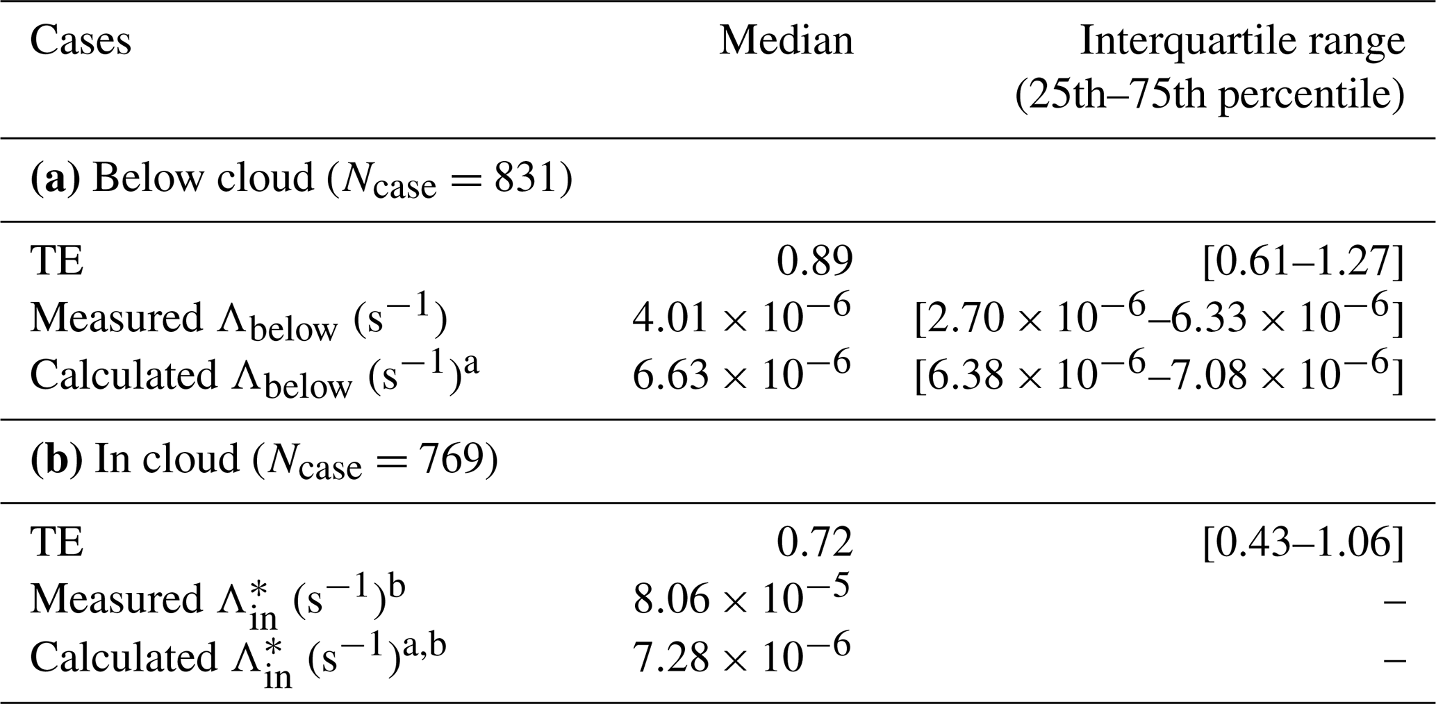
^a Calculated using the FLEXPART scheme. ^b Overall median value.

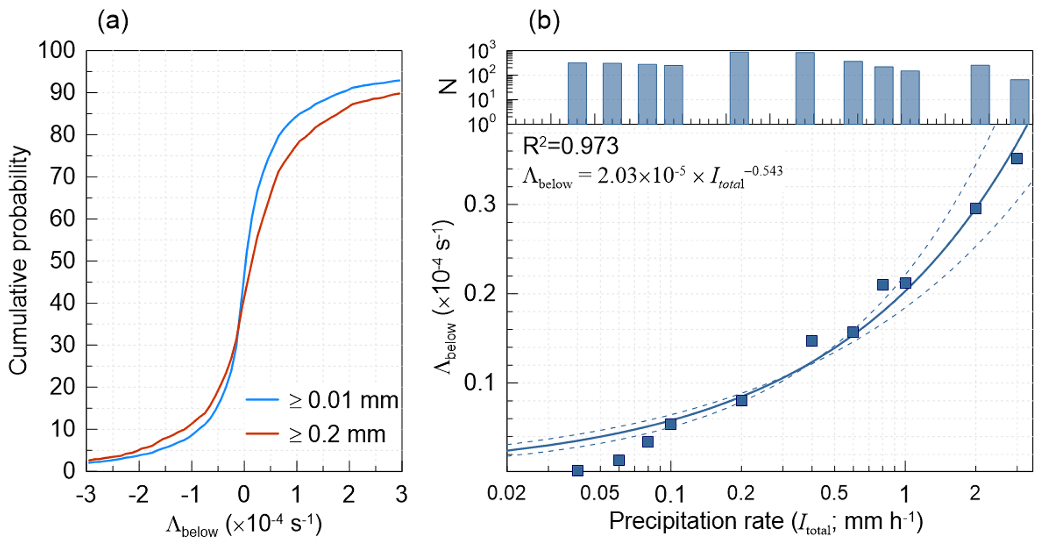
Figure 5 (a) Empirical cumulative distribution plot of measured below-cloud scavenging coefficients (Λ_below; s⁻¹), depending on the precipitation rate (≥0.01 and ≥0.2 mm h⁻¹). (b) Median measured Λ_below as a function of the precipitation intensity (mm h⁻¹) of 11 bins. The dashed line indicates the fit from the equation. The upper panel of (b) shows the number of hourly data points for each bin for I_total. The 11 bins consist of 0.01–0.04, 0.04–0.06, 0.06–0.08, 0.08–0.1, 0.1–0.2, 0.2–0.4, 0.4–0.6, 0.6–0.8, 0.8–1, 1–2, and 2–3 mm h⁻¹.

Figure 5a indicates the empirical cumulative density function for the measured Λ_below from 869 cases. Although a substantial fraction of Λ_below values were close to zero (or negative), the median Λ_below was significantly different from zero and also positive ($\mathrm{7.9}\times {\mathrm{10}}^{-\mathrm{6}}$ s⁻¹), with an interquartile range of $-\mathrm{1.7}\times {\mathrm{10}}^{-\mathrm{5}}$ to $\mathrm{5.3}\times {\mathrm{10}}^{-\mathrm{5}}$ s⁻¹. Negative Λ_below values have been reported in previous studies (Laakso et al., 2003; Pryor et al., 2016; Zikova and Zdimal, 2016); therefore, we assumed that these negative values reflected the uncertainty in the measurements and/or inclusion of BC, which might be continuously supplemented in air masses. As the threshold of I_total increased from 0.01 (all cases) to 0.2 mm h⁻¹ (median), Λ_below values were increased by a factor of 2.5 to $\mathrm{2.0}\times {\mathrm{10}}^{-\mathrm{5}}$ s⁻¹ ($-\mathrm{2.5}\times {\mathrm{10}}^{-\mathrm{5}}$ s⁻¹ to $\mathrm{9.0}\times {\mathrm{10}}^{-\mathrm{5}}$ s⁻¹). Using these obviously increasing tendencies of Λ_below according to I_total, we determined the empirical fitting equation by investigating the relationship between median Λ_below and each bin of I_total. Figure 5b indicates Λ_below as a function of I_total based on its allocation to 11 logarithmic bins. Because the estimated I_total bins covered the I_total ranges, 0.03 to 2.0 mm h⁻¹ (5th percentile to 95th percentile), this exponential fitting equation ($A\times I_{\text{total}}^B$) could be representative for below-cloud scavenging over East Asia. The constant A and exponent B with a 95 % confidence interval were $\mathrm{2.0}\times {\mathrm{10}}^{-\mathrm{5}}$ (1.9–$\mathrm{2.2}\times {\mathrm{10}}^{-\mathrm{5}}$) and 0.54 (0.46–0.64), respectively. Instead of the SED equation shown in Fig. 2, we chose the exponential fitting equation because of its higher R² (0.973) compared to that from SED fitting (0.903), as well as being widely used in previous studies.

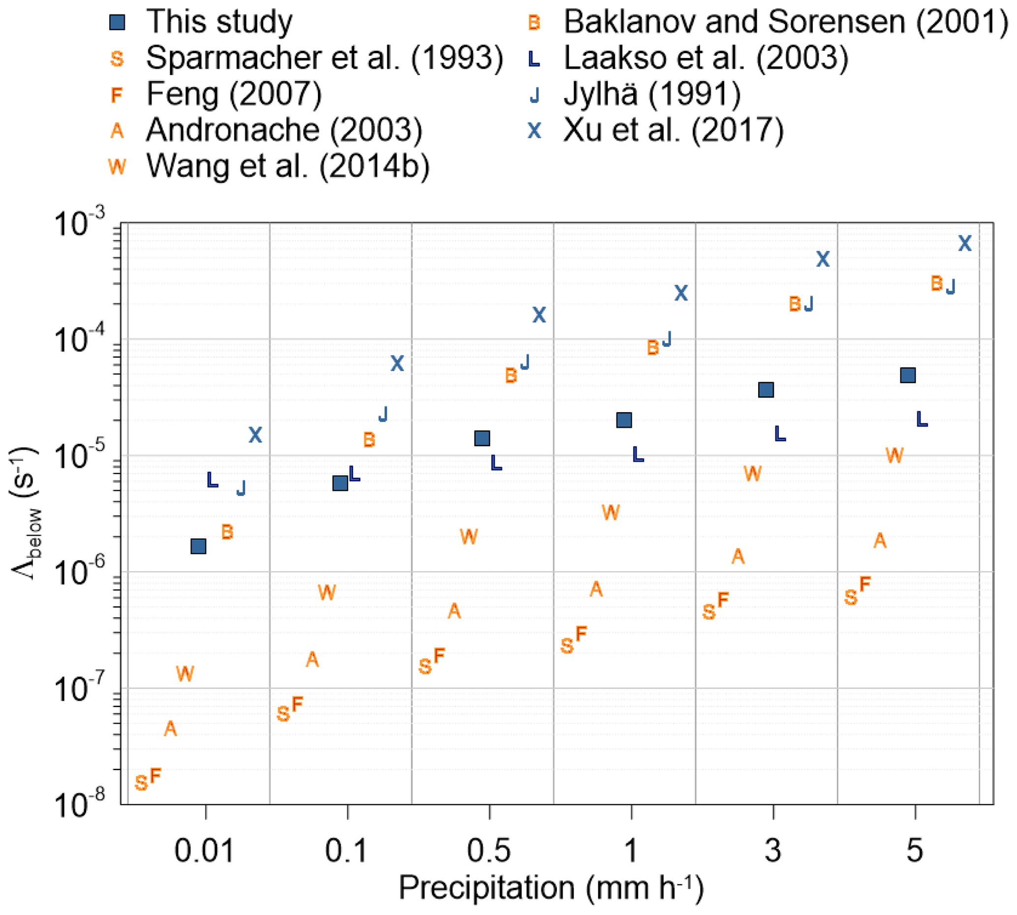
Figure 6 Variations in calculated and measured below-cloud scavenging coefficients (Λ_below; s⁻¹) depending on the precipitation intensity (mm h⁻¹). Orange and blue symbols depict the Λ_below equation based on theoretical calculations and observation data, respectively. The diameter of BC was assumed to be approximately 200 nm in the calculation.

Figure 6 shows a comparison of Λ_below calculated by using equations from previous studies with those derived from our equation and by assuming that the BC size was approximately 200 nm. To compare the measured Λ_below, we used the mean fractional bias (MFB; $\mathrm{2}\times [A-B]/[A+B]$), where A and B denote calculated and measured Λ_below value, respectively. Our newly measured Λ_below values were located in the intermediate range of the calculated Λ_below, and the mean deviations between the measured and all calculated values were relatively constant with increasing I_total because the mean absolute MFBs were slightly increased from 1.4 to 1.6. It should be noted that Λ_below from Laakso et al. (2003), which is the default scheme for below-cloud scavenging in the FLEXPART model version 10 or higher (Grythe et al., 2017), showed fairly good agreement with our measured Λ_below among the calculated values (mean absolute MFB of 0.68). MFB was positive at low I_total, but the opposite tendency was observed for I_total at ∼0.1 mm h⁻¹, suggesting that Λ_below might be converged within a similar range when we consider the range of I_total. Although calculated Λ_below from Laakso et al. (2003) showed good agreement with our results, the median calculated Λ_below ($\mathrm{6.6}\times {\mathrm{10}}^{-\mathrm{6}}$ s⁻¹) was overestimated compared to the measured value ($\mathrm{4.0}\times {\mathrm{10}}^{-\mathrm{6}}$ s⁻¹) by a factor of 1.7 when we recalculated the below-cloud cases only. The MFBs from other schemes were too high or low to declare reasonable results. For example, the Λ_below of secondary ions in Beijing (Xu et al., 2017) had the highest MFB (1.68), and although the diameter ranges were larger (∼500 nm) than those of BC, the effect of the differences in diameter might be negligible because significant difference in Λ_below between two diameters were not observed (less than 30 %) when applied to Laakso et al. (2003).

3.5 In-cloud scavenging coefficient (Λ_in)

Compared to Λ_below, the calculation of Λ_in is much more complicated because many factors can influence the in-cloud scavenging process, such as precipitation, total cloud cover (TCC), the specific cloud total water content (CTWC), and so on. A detailed description of the complicated equation for Λ_in in FLEXPART v10 is presented in Grythe et al. (2017), and the equation for Λ_in can be simply expressed as follows:

$$\begin{array}{}\text{(4)}& {\mathrm{\Lambda }}_{\text{in}}={\displaystyle \frac{i_{\text{cr}}\cdot F_{\text{nuc}}\cdot I_{\text{total}}\cdot \text{TCC}}{\text{CTWC}\cdot f_{\mathrm{g}}}},\end{array}$$

where i_cr and F_nuc are the cloud water replenishment factor (6.2; default value) and the nucleation efficiency, respectively. It should be mentioned that Λ_in was also calculated by following the FLEXPART scheme using the ERA5 meteorological data ($\mathrm{0.25}{}^{\circ }\times \mathrm{0.25}{}^{\circ }$) with HYSPLIT backward trajectory instead of the FLEXPART simulation ($\mathrm{1}{}^{\circ }\times \mathrm{1}{}^{\circ }$) to reflect the local variability of meteorological variables. Among the 769 cases for in-cloud cases, Eqs. (2) and (3) were also used to calculate TE for in-cloud only cases by substituting Λ with calculated Λ_in. Unlike the hourly measured Λ_below calculated by optimization, the only overall median Λ_in (${\mathrm{\Lambda }}_{\text{in}}^{\ast }$) for in-cloud cases was calculated using Eq. (3) because Λ_in cannot be constrained by a specific variable.

The calculated ${\mathrm{\Lambda }}_{\text{in}}^{\ast }$ ($\mathrm{7.28}\times {\mathrm{10}}^{-\mathrm{6}}$ s⁻¹) from the FLEXPART scheme (hereafter calculated as ${\mathrm{\Lambda }}_{\text{in}}^{\ast }$) was underestimated by 1 order of magnitude compared to our measured ${\mathrm{\Lambda }}_{\text{in}}^{\ast }$ ($\mathrm{8.06}\times {\mathrm{10}}^{-\mathrm{5}}$ s⁻¹). When FLEXPART TE for in-cloud cases (all cases) was recalculated by considering a 10 (5) times higher Λ_in, the median FLEXPART TE was 0.73 (0.79), which was much closer to the measured TE (both 0.72). Although the grid size of the meteorological input data for the two approaches did not match, the underestimation of the in-cloud scavenging scheme in FLEXPART was confirmed. Grythe et al. (2017) reported an overestimation of observed BC (a factor of 1.68) due to inaccurate emission sources rather than underestimated in-cloud removal efficiencies. Although the effect of BC particle dispersion on adjacent grid cells was neglected in our approach, the underestimation of in-cloud scavenging coefficients was obvious because the accuracy of the emission inventory did not affect the measured ${\mathrm{\Lambda }}_{\text{in}}^{\ast }$. Looking more closely into the sites, the calculated ${\mathrm{\Lambda }}_{\text{in}}^{\ast }$ at Noto was remarkably underestimated by 1 order of magnitude, followed by Gosan (∼90 %) and Baengnyeong (∼43 %), similar to the order of the wet removal efficiency. It should be noted that the coefficient of variation (CV; standard deviation divided by the mean) of calculated ${\mathrm{\Lambda }}_{\text{in}}^{\ast }$ was much lower (0.23) than the measured ${\mathrm{\Lambda }}_{\text{in}}^{\ast }$ (0.78), indicating that the calculated ${\mathrm{\Lambda }}_{\text{in}}^{\ast }$ did not accurately represent the actual regional difference in the real world. Among the meteorological input variables in Eq. (4), the CV of I_total was the highest at 0.22, which was similar to the CV of the calculated ${\mathrm{\Lambda }}_{\text{in}}^{\ast }$, followed by CTWC (0.08), f_g (0.03), and TCC (0.02), suggesting that the difference in calculated ${\mathrm{\Lambda }}_{\text{in}}^{\ast }$ could be partially explained by I_total rather than other variables. Among the meteorological variables that were not considered in Eq. (4), the convective available potential energy (CAPE), which is well known as an indicator of vertical instability (Mori et al., 2014), had the highest CV at 0.31.

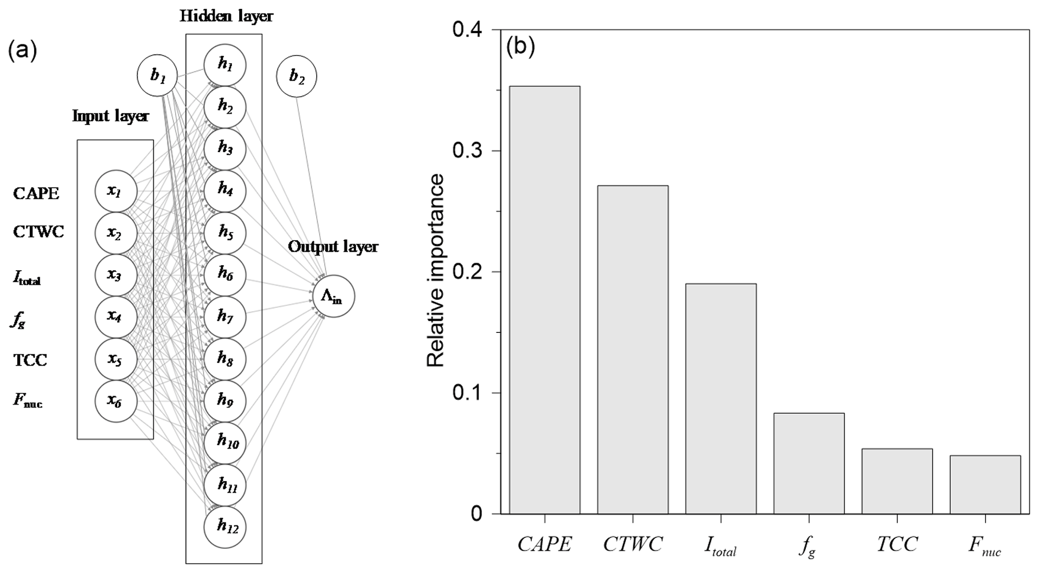
Figure 7 (a) Schematic of an artificial neuron network (ANN) model with 12 nodes of a single hidden layer. (b) The relative importance of six meteorological input variables used for calculating in-cloud scavenging coefficients in the FLEXPART model (except for CAPE), using Garson's algorithm implemented in the “NeuralNetTools” package in R. CAPE, CTWC, I_total, f_g, TCC, and F_nuc represent the convective available potential energy, specific cloud total water content, precipitation rate, fraction of a subgrid in a grid cell (see text for details), total cloud cover, and nucleation efficiency, respectively.

We employed an artificial neural network (ANN) to compare the importance of CAPE with other considered meteorological input variables to determine the hourly Λ_in instead of ${\mathrm{\Lambda }}_{\text{in}}^{\ast }$. We applied a stricter selection for in-cloud cases, i.e., only when in-cloud scavenging occurred less than three times (i.e., in three cells) in a single case, regardless of the number of below-cloud occurrences. Because the effect of below-cloud scavenging was successfully excluded from the TE using the derived equation for Λ_below in the previous section, the Λ_in in less than three in-cloud cases can also be calculated by optimization based on the remaining TE. We applied a threshold of three cases here because the number of data (230 cases) was sufficient to conduct statistical analysis, while the optimization uncertainty could be reduced to its minimum. The ANN model was trained using six meteorological variables (CAPE, CTWC, f_g, F_nuc, I_total, and TCC), and all variables were normalized by the minimum and maximum of each variable $\left(\right[x-min\left(x\right)]/[max\left(x\right)-min\left(x\right)\left]\right)$. To determine the optimal node numbers in the hidden layer, we applied the “caret” package of the R function that contains several sets of machine-learning modes and validation tools, (https://cran.r-project.org/web/packages/caret/caret.pdf, last access: 20 October 2020) and we adopted a method from the “neuralnet” package that is a fit for a multi-hidden layer. By varying the size (node number) from five to 20 and using k-fold cross validation, the selected cases were randomly divided by a ratio of 3:1 into training (172 data points) and validation data (58 data points). Garson's algorithm in the “NeuralNetTools” package was used to identify the relative importance of six input variables in the final neural network (Garson, 1991). The model's performance was assessed from these independent validation data by calculating the root mean squared error. The optimal number of nodes in the hidden layer was 12 (Fig. 7a).

Figure 7b shows the relative importance of input variables for calculating Λ_in using Garson's algorithm. The most important input variable was CAPE, with a value of 35 %, followed by CTWC, I_total, and so on, thus confirming that CAPE should be considered in the Λ_in calculation. Typically, enhancing wet removal by convective clouds successfully reduces the aloft BC concentration in the free troposphere (Koch et al., 2009). Therefore, the convective process is important in tropical regions but has a slightly lower impact at midlatitudes (Luo et al., 2019; Grythe et al., 2017; Xu et al., 2019). Moreover, previous studies have highlighted convective scavenging to be a key parameter in determining the BC concentration in model simulations (Lund et al., 2017; Xu et al., 2019), and the role of wet removal by convective clouds might be significant when most air masses travel above the planetary boundary layer. Unfortunately, the current version of FLEXPART does not implement convective scavenging (Philipp and Seibert, 2018), which could be a plausible reason for the underestimation of calculated Λ_in. Although the relative importance of each variable cannot be parameterized to calculate Λ_in, this approach highlights that CAPE is one of the key factors for determining Λ_in over East Asia. In the future, more information might be required to evaluate the in-cloud scavenging scheme using the Weather Research and Forecasting (WRF)–FLEXPART at a higher resolution in further studies, since a 0.25^∘ grid size is still not sufficient to reproduce convective clouds (typically 10 km or less).

4 Conclusions

The wet removal rates and scavenging coefficients for BC were investigated by the term of ΔBC∕ΔCO ratios from long-term, best-effort observations at three remote sites in East Asia (Baengnyeong and Gosan in South Korea and Noto in Japan). By combining the backward trajectories covering the past 72 h, the accumulated precipitation along trajectories (APT), and the transport efficiency (TE; [ΔBC∕ΔCO]${}_{\text{APT}>\mathrm{0}}/[\mathrm{\Delta }\text{BC}/\mathrm{\Delta }\text{CO}{]}_{\text{APT}=\mathrm{0}}$), BC wet removal efficiency was assessed as an aspect of the pathway of trajectories, including the successful identification of below- and in-cloud cases. The overall wet removal rates as a function of APT, the half-life and the e-folding lifetime were similar to those of previous studies but showed large regional differences depending on the measurement site. The difference in the wet removal rate, depending on the measurement site, can be explained by the different meteorological conditions such as the precipitation rate, cloud cover, total column cloud water, and cloud bottom height. The differences in regional and seasonal wet removal rates might be influenced by the frequency of exposure to below- and in-cloud scavenging conditions during transport as well as the magnitude of the aging process causing the different coating thicknesses because the thick-coated BC particles are preferentially removed due to cloud processes. By discriminating below- and in-cloud dominant cases according to cloud vertical information from ERA5 pressure level data, scavenging coefficients for below-cloud (Λ_below) and in-cloud (${\mathrm{\Lambda }}_{\text{in}}^{\ast }$) cases were simply converted from the measured TE values. The calculated Λ_below from the FLEXPART scheme was overestimated by a factor of 1.7 compared to the measured Λ_below, although the measured Λ_below showed good agreement with the below-cloud scheme in FLEXPART among the reported scavenging coefficients. In contrast to Λ_below, the calculated ${\mathrm{\Lambda }}_{\text{in}}^{\ast }$ from the FLEXPART scheme was highly underestimated by 1 order of magnitude, compared to measured ${\mathrm{\Lambda }}_{\text{in}}^{\ast }$, suggesting that the current in-cloud scavenging scheme did not represent regional variability. By diagnosing the relative importance of the input variables using the artificial neuron network (ANN), we found that the convective available potential energy (CAPE), which is an indicator of vertical instability, should be considered to improve the in-cloud scavenging scheme because convective scavenging could be regarded as a key parameter for determining the accurate BC concentration in a model. This study could contribute not only to improving the below-cloud scavenging scheme implemented in a model, especially for FLEXPART, but also to providing evidence for complementary in-cloud scavenging schemes by considering the convective scavenging process. For the first time, these results suggest a novel and straightforward approach for evaluating the wet scavenging scheme in various models and for enhancing the understanding of BC behavior by excluding the effects of inaccurate emission inventories.