the Creative Commons Attribution 4.0 License.
the Creative Commons Attribution 4.0 License.
 | 09 Nov 2020
Impacts of global NOx inversions on NO2 and ozone simulations
Daven K. Henze
Owen R. Cooper
Jessica L. Neu
Tropospheric NO2 and ozone simulations have large uncertainties, but their biases, seasonality, and trends can be improved with NO2 assimilations. We perform global top-down estimates of monthly NOx emissions using two Ozone Monitoring Instrument (OMI) NO2 retrievals (NASAv3 and DOMINOv2) from 2005 to 2016 through a hybrid 4D-Var/mass balance inversion. Discrepancy in NO2 retrieval products is a major source of uncertainties in the top-down NOx emission estimates. The different vertical sensitivities in the two NO2 retrievals affect both magnitude and seasonal variations of top-down NOx emissions. The 12-year averages of regional NOx budgets from the NASA posterior emissions are 37 % to 53 % smaller than the DOMINO posterior emissions. Consequently, the DOMINO posterior surface NO2 simulations greatly reduced the negative biases in China (by 15 %) and the US (by 22 %) compared to surface NO2 measurements. Posterior NOx emissions show consistent trends over China, the US, India, and Mexico constrained by the two retrievals. Emission trends are less robust over South America, Australia, western Europe, and Africa, where the two retrievals show less consistency. NO2 trends have more consistent decreases (by 26 %) with the measurements (by 32 %) in the US from 2006 to 2016 when using the NASA posterior emissions. The performance of posterior ozone simulations has spatial heterogeneities from region to region. On a global scale, ozone simulations using NASA-based emissions alleviate the double peak in the prior simulation of global ozone seasonality. The higher abundances of NO2 from the DOMINO posterior simulations increase the global background ozone concentrations and therefore reduce the negative biases more than the NASA posterior simulations using GEOS-Chem v12 at remote sites. Compared to surface ozone measurements, posterior simulations have more consistent magnitude and interannual variations than the prior estimates, but the performance from the NASA-based and DOMINO-based emissions varies across ozone metrics. The limited availability of remote-sensing data and the use of prior NOx diurnal variations hinder improvement of ozone diurnal variations from the assimilation, and therefore have mixed performance on improving different ozone metrics. Additional improvements in posterior NO2 and ozone simulations require more precise and consistent NO2 retrieval products, more accurate diurnal variations of NOx and VOC emissions, and improved simulations of ozone chemistry and depositions.
- Article
(5616 KB) - Full-text XML
-
Supplement
(3379 KB) - BibTeX
- EndNote


Tropospheric ozone is a harmful secondary air pollutant affecting human health, sensitive vegetation, and ecosystems (NRC, 1991; Monks et al., 2015). Long-term ozone (O3) exposure is estimated to cause 1.04–1.23 million respiratory deaths in adults (Malley et al., 2017). Short-term exposure to high ambient ozone concentrations is associated with respiratory and cardiovascular mortality (Turner et al., 2016; Fleming et al., 2018). Accurate simulations of ozone in highly polluted regions are important for better pollution forecasts and more effective emission regulations. Tropospheric ozone is formed through photochemical reactions between nitrogen oxide (NOx = NO + NO2), carbon monoxide (CO), methane (CH4), and volatile organic compounds (VOCs) in the presence of sunlight (Crutzen, 1973; Derwent et al., 1996). These precursor gases are mainly emitted from fossil-fuel combustion, biomass burning, oil and gas production, industry, agriculture, and biogenic activities. Tropospheric ozone can also be transported from the stratosphere through stratosphere–troposphere exchange (Stohl et al., 2003; Hsu and Prather, 2009; Stevenson et al., 2006; Lu et al., 2019), but this magnitude is smaller than the amount from chemical production by a factor of 5–7 (Young et al., 2013). Ozone is removed from the troposphere through deposition (Fowler et al., 2009), photodissociation, and reactions with HO2, NO2, unsaturated VOCs, halogens, and aerosols (Crutzen, 1973).
From 1850 to 2000, global mean tropospheric ozone burden has increased by 29 % (Young et al., 2013). Human activities are major sources of ozone precursor gases, contributing to a 9 % (24.98 Tg) increase of the global tropospheric ozone burden from 1980 to 2010 (Zhang et al., 2016). Ozone formation and trends depend nonlinearly on the local relative abundances of NOx and VOCs and the radiative regime in which these occur. Previous studies have shown that changes in surface ozone are dominated by regional emission trends of precursor gases (Zhang et al., 2016). At the global scale, 77 % of NOx emissions are from anthropogenic sources, according to the HTAP 2010 inventory (Janssens-Maenhout, 2015). Anthropogenic NOx emissions have been decreasing in North America and Europe due to transportation and energy transformations (Simon et al., 2015) but have been increasing in China up until 2011 according to bottom-up emission inventories (Liu et al., 2016; Hoesly et al., 2018). Top-down NOx emission estimates using satellite observations from the Ozone Monitoring Instrument (OMI) showed a similar turning point in China (Miyazaki et al., 2017; Qu et al., 2017), but there was a slowdown in reductions in the US compared to bottom-up estimates (Miyazaki et al., 2017; Jiang et al., 2018). However, in India and the Middle East, where ozone production is more efficient than higher-latitude regions (Zhang et al., 2016), NO2 column densities from OMI are continuing to increase (Krotkov et al., 2016).
Top-down methods have the advantage of being able to update emissions in a more timely fashion than the bottom-up approaches; still, top-down approaches can contain large differences and uncertainties. For instance, the magnitude of tropospheric NO2 column densities from two global retrievals from the National Aeronautics and Space Administration (NASA) and the Royal Netherlands Meteorological Institute (KNMI) differ by 50 % and have different trends at the regional scale (Zheng et al., 2014; Canty et al., 2015; Qu et al., 2017). These differences in column densities can propagate to differences in top-down NOx emission estimates (e.g., Miyazaki et al., 2017; Qu et al., 2017). In this study, we assess the importance of these discrepancies in NOx emissions for the simulation of ozone. We derive global top-down NOx emissions from 2005 to 2016 using two widely used products (OMNO2 v3 and Dutch OMI NO2 (DOMINO) v2) based on the same inversion process for consistent evaluations (Sect. 3). We also evaluate a new OMI NO2 retrieval product, the Quality Assurance for the Essential Climate Variables (QA4ECV) (Boersma et al., 2018), and apply it to derive monthly NOx emissions in 2010. We do not repeat our entire set of ozone evaluations with this product given that its magnitude and seasonality do not significantly differ from the other two products. We further explore the impact of adjusting NOx emissions on ozone simulations by evaluating the ozone simulations produced from bottom-up and top-down NOx emissions against global surface measurements from the Tropospheric Ozone Assessment Report (TOAR) database and the China National Environmental Monitoring Center (CNEMC) network.
In addition to local sources, the lifetime of ozone (∼22 d on global average) is sufficiently long enough for intercontinental transport (UNECE, 2010). Consequently, every country is an exporter as well as an importer of ozone pollution. Transport from East Asia can be an important contributor to ozone exceedances in the western US (Goldstein et al., 2004; Zhang et al., 2009, 2014; Fiore et al., 2014; Verstraeten et al., 2015; Lin et al., 2017; Jaffe et al., 2018). The influence of intercontinental ozone transport is strongest in spring and summer, when background ozone concentrations reach 50 ppbv at the west coast of the US (Jaffe et al., 2018). The impact of background ozone is increasingly important and challenging due to the decreased local sources of precursor gases in the US (Hoesly et al., 2018) and the recent stricter ozone standard in the US. This involved lowering the annual fourth highest maximum daily 8 h average ozone concentration from 75 to 70 ppbv in 2015 (Cooper et al., 2015). Optimization of NOx emissions in the upwind regions can improve remote ozone simulations in downwind regions after transport of intercontinental pollution plumes from the free troposphere to the surface (Zhang et al., 2008; Verstraeten et al., 2015). Therefore, we also evaluate the model simulations of remote ozone at the west coast of the United States using bottom-up and top-down NOx emissions in Sect. 4.
2.1 GEOS-Chem and its adjoint model
The GEOS-Chem adjoint model (Henze et al., 2007) v35k is used to derive global NOx emission estimates at resolution. It was developed for inverse modeling of aerosol and gas emissions using the 4D-Var method by Henze et al. (2007, 2009) based on version 8 of GEOS-Chem, with bug fixes and updates up to version 10. Simulations in this study are driven by Modern-Era Retrospective analysis for Research and Applications, Version 2 (MERRA-2) meteorological fields from the NASA Global Modeling and Assimilation Office (GMAO). Anthropogenic emissions of NOx, SO2, NH3, CO, NMVOCs (non-methane volatile organic compounds), and primary aerosol from the HTAP 2010 inventory version 2 (Janssens-Maenhout et al., 2015) are used to drive all prior simulations from 2005 to 2017. The diurnal variation of NOx emissions is derived from EDGAR hourly variations (http://wiki.seas.harvard.edu/geos-chem/index.php/Scale_factors_for_anthropogenic_emissions3Diurnal_Variation) and is not optimized in the inversion. The use of non-anthropogenic emissions and other setups follows Qu et al. (2017, 2019a, b). In the following analyses, we refer to this model as “GC-adj.”
GC-adj does not include several halogen chemistry mechanisms that affect ozone depletions primarily over the oceans (Sherwen et al., 2016a; Wang et al., 2019) and at high-altitude regions (Sherwen et al., 2016a). Given their impact on the global background ozone concentrations, we also use GEOS-Chem v12.1.1 to evaluate ozone simulations at resolution driven by the MERRA-2 meteorological fields. The chemistry updates include the stratospheric chemistry from the unified tropospheric–stratospheric chemistry extension (UCX) (Eastham et al., 2014), halogen chemistry (Bell et al., 2002; Parrella et al., 2012; Sherwen et al., 2016a, 2016b; Schmidt et al., 2016; Sherwen et al., 2017), and updated isoprene and monoterpene chemistry (Chan Miller et al., 2017; Fisher et al., 2016; Marais et al., 2016; Travis et al., 2016). The Harvard–NASA Emissions Component (HEMCO) is employed to process emissions in this version of GEOS-Chem (Keller et al., 2014). We use 72 levels of vertical grid and global anthropogenic emissions from the Community Emissions Data System (CEDS) (Hoesly et al., 2018). Top-down NOx emissions derived by using GC-adj are also input to this model to evaluate the impact of NO2 data assimilation on ozone simulations under different chemical mechanisms. We refer to this model as “GCv12” in this article.
For each NOx emission dataset, the model spin-up time is 6 months, starting from July 2005. Therefore, we derive NOx emissions from 2005 but only evaluate simulations with measurements from 2006. To avoid high biases when comparing simulated ozone averaged over the first vertical model layer (∼100 m in box height) with surface measurements, 2 m ozone mixing ratios are calculated by scaling simulated ozone mixing ratios in the first layer using adjusted dry deposition velocities at 2 m following Zhang et al. (2012) and Lapina et al. (2015).
2.2 Satellite observations and global top-down NOx emissions
We estimate global top-down NOx emissions at the surface from 2005 to 2016 at resolution using tropospheric NO2 column densities from OMI. OMI is an ultraviolet/visible nadir solar backscatter spectrometer aboard the NASA Aura satellite. It has a local overpass time of about 13:45 LT and a nadir resolution of 13 km×24 km. OMI was launched in July 2004 and has provided operational data products since October 2004. Two level-2 NO2 retrieval products are used to derive long-term top-down NOx emissions in this study: the NASA standard product OMNO2 version 3 (Krotkov et al., 2017) and the DOMINO version 2 from KNMI (Boersma et al., 2011). A new OMI NO2 retrieval, the Quality Assurance for the Essential Climate Variables (QA4ECV) (Boersma et al., 2018), has recently become available. This product is jointly developed by KNMI, the Belgian Institute for Space Aeronomy (BIRA-IASB), University of Bremen, Max Plank Institute for Chemistry, and Wageningen University. We evaluate the magnitude of NO2 column densities and the seasonality of posterior NOx emissions in 2010 from this product. We screen all OMI NO2 retrievals using data quality flags and by the criteria of positive tropospheric column, cloud fraction <0.2, solar zenith angle , and viewing zenith angle . We excluded all retrievals that are affected by row anomaly.
We converted GEOS-Chem NO2 vertical column densities (VCDs) to slant column densities (SCDs) using scattering weight from the OMI retrievals and then compared GEOS-Chem SCDs with SCDs retrieved from OMI. The scattering weights are the product of the averaging kernels and the air mass factor (AMF) (Palmer et al., 2001; Chance and Martin, 2017). A cost function is defined as the observation-error-weighted differences between simulated and retrieved NO2 SCDs plus the prior emissions error-weighted departure of the emission scaling factors from the prior estimates. We minimize the cost function using the quasi-Newton L-BFGS-B gradient-based optimization technique (Byrd et al., 1995; Zhu et al., 1994), in which the gradient of the cost function with respect to the control parameter is calculated using the adjoint method. Details of the assimilation of NO2 SCDs, how vertical sensitivities of satellite retrievals are accounted for, and the hybrid 4D-Var/mass balance inversion of NOx emissions are described in Qu et al. (2017). We use top-down NOx emissions estimated from the NASA standard product and the DOMINO product (Qu et al., 2020a, b) in the evaluations of ozone simulations.
2.3 Surface measurements
We evaluate surface NO2 simulations with measurements from the Environmental Protection Agency (EPA) Air Quality System (AQS) in the US and the China National Environmental Monitoring Center (CNEMC) network in China. The city monitoring sites included in the analysis represent either urban background or the averaged pollutant concentrations over the city. Simulated ozone mixing ratios from 2006 to 2016 are compared to surface observations from the TOAR Surface Observation Database (Schultz et al., 2017a) at the global scale and the CNEMC network in China. TOAR has produced a relational database of global surface ozone observations at all available sites; see Gaudel et al. (2018) for illustrations of the global coverage of the TOAR data. Pre-compiled TOAR data (https://doi.org/10.1594/PANGAEA.876108, available from 1995 to 2014, Schultz et al., 2017b) at each individual site are used in this study. Given the sparse TOAR data coverage of only 32 sites over China, hourly surface ozone measurements from the CNEMC (http://106.37.208.233:20035/, last access: 1 November 2020) are used to evaluate simulations in China from 2014 to 2016. The CNEMC national network was designed for urban and suburban air pollution monitoring. The archive contains hourly observations of ozone, carbon monoxide, nitrogen dioxide, sulfur dioxide, and fine particulate matter across mainland China since 2013.
2.4 Ozonesonde measurements
Ozone profile measurements from the Intercontinental Chemical Transport Experiment Ozonesonde Network Study (IONS-2010) (Cooper et al., 2011) are used to evaluate the continental inflow of ozone along the west coast of the United States, where air masses are not influenced by recent US emissions. IONS-2010 was a component of the California Research at the Nexus of Air Quality and Climate Change (CalNex) 2010 experiment (Ryerson et al., 2013) and was a continuation of previous IONS experiments to measure tropospheric ozone variability across North America (Thompson et al., 2007, 2008; Cooper et al., 2007). Balloon-borne electrochemical cell sensors were used to measure ozone profiles with an accuracy of ±10 % in the troposphere (Johnson et al., 2002; Smit et al., 2007). All six sites in California from IONS-2010 (referred to as Trinidad Head, Point Reyes, Point Sur, San Nicolas, Joshua Tree, and Shasta) are included in this study. These measurements are made in the mid-afternoon (95 % occurring between 14:00 and 16:59 LT) over a 6-week period from 10 May to 19 June 2010. There are 34–37 profiles for all sites except for San Nicolas Island, where only 26 profiles are available due to multiple instrument failures. Measurements made between 700 and 800 hPa are used to evaluate remote-ozone simulations.
Differences between the prior and posterior NOx emission estimates are mainly driven by the differences between simulated and retrieved tropospheric NO2 vertical column densities (VCDs), which are compared in Sect. S1 in the Supplement. The GEOS-Chem NO2 SCDs converted using scattering weight from the NASA product are larger than the SCDs calculated using the DOMINO scattering weight and the same GEOS-Chem VCDs (See Fig. S2). These can be explained by the use of different surface albedo and cloud product in the two retrievals. The retrieved NO2 SCDs from the NASA product are mostly smaller than the DOMINO retrieval except for some regions between 40 and 60∘ N in January 2010. The smaller magnitude in OMI SCD and the larger magnitude in GEOS-Chem SCD using the NASA scattering weight lead to a smaller magnitude of posterior NOx emissions than inversions from the DOMINO product. The cost function has reduced by 6 %–29 % in the monthly inversion.
3.1 Annual average
As shown in Table 1, the global budgets of NOx emissions from the NASA posterior emissions in 2010 are 0.7 % smaller than the prior emissions; DOMINO posterior emissions are 18 % larger than the prior emissions; QA4ECV posterior emissions are 11 % larger than the prior emissions. The positive increment in the DOMINO posterior emissions is consistent with the +26 % increments of 10-year mean posterior NOx emissions in Miyazaki et al. (2017). The annual global NOx emissions from Miyazaki et al. (2017) are between 46.7 and 50.9 TgN yr−1 from 2005 to 2014, which are within 31 % from the DOMINO posterior emissions in 2010 in this study.
Table 1Total NOx emission (anthropogenic plus natural) budgets in 2010 (TgN yr−1).
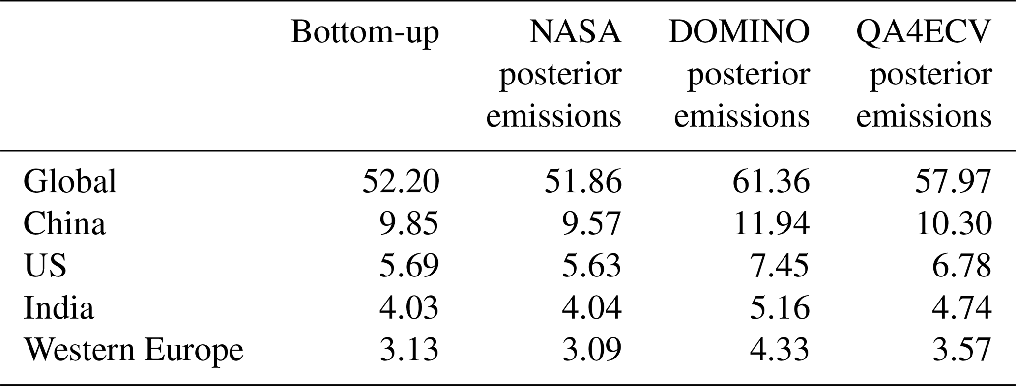
As shown in Fig. 1, the NASA posterior NOx emissions are less than the prior NOx emissions in the northeast US, northeast China, and southeast China. The DOMINO posterior NOx emissions are larger than the prior emissions in most regions except for northern Mexico and most parts of the tropics. The QA4ECV posterior NOx emissions have more consistent negative increments in eastern China with the NASA posterior emissions and more consistent positive increments in the United States, India, Europe, and Australia with the DOMINO posterior emissions. At the regional scale, NASA posterior increments are −3 % in China, −1 % in the US, +0.3 % in India, and −1 % in western Europe. The increments from the DOMINO posterior emissions are +21 % in China, +31 % in the US, +28 % in India, and +38 % in western Europe. The different changing directions in the above two posterior NOx emissions are consistent with the reportedly higher magnitude of NO2 column densities in the DOMINO product than the NASA product in densely populated and industrial regions (Zheng et al., 2014; Canty et al., 2015; Qu et al., 2017). The increments from the QA4ECV posterior emissions are +5 % in China, +19 % in the US, +18 % in India, and +14 % in western Europe.
To evaluate the magnitude of the posterior NOx emissions, we compare simulations of surface NO2 concentrations using the NASA- and DOMINO-based NOx emissions with surface measurements in the US and China. Surface NO2 simulations at coarse resolution are usually biased low compared to measurements at urban sites, due to the short lifetime of NOx. We therefore start with analyzing this resolution error by generating high-resolution pseudo surface measurements at and compare them with low-resolution model simulations at . We generate high-resolution surface NO2 concentrations by scaling simulated surface NO2 concentrations at grid cells by the ratio of OMI NO2 column density gridded at to the OMI NO2 column density gridded at grid cell. We identify grid cells that include surface monitoring sites and treat downscaled surface NO2 concentrations at these grid cells as the pseudo surface measurements. Comparisons of pseudo surface measurements and NO2 simulations at purely reflect differences caused by comparing NO2 concentrations at with higher-resolution surface measurements at urban regions. The mean of the pseudo NO2 measurements is 32 % higher than the low-resolution simulations in the US, and it is 18 % higher than the low-resolution simulations in China. The real surface measurements, which represent a single point within the grid cell, are expected to have even larger biases than the values calculated here, where we assume the measurements are at grid cells. The smaller bias in China in comparison to the US is related to the higher background NO2 concentrations in China.
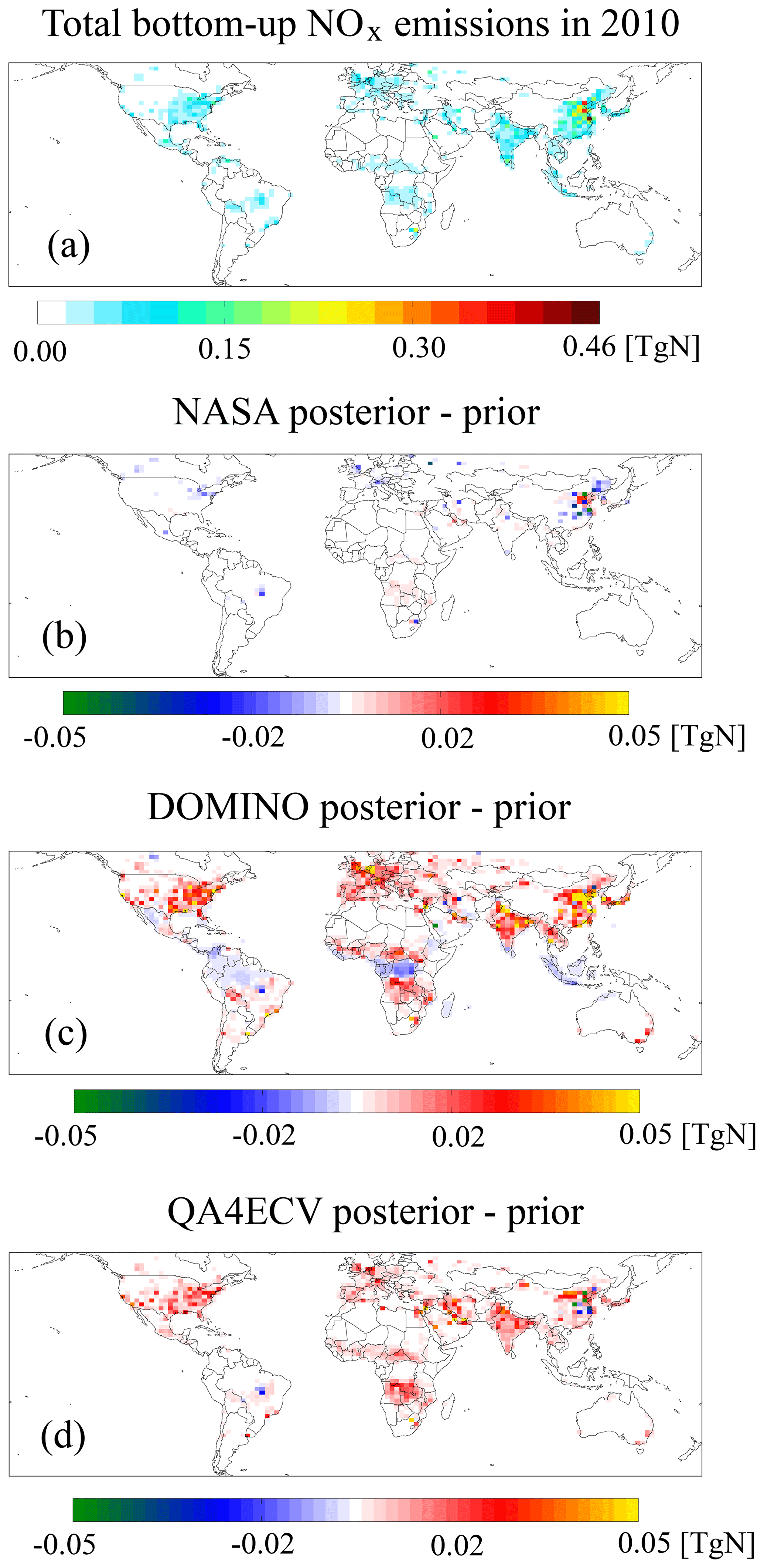
Figure 1(a) Global total NOx emissions from the bottom-up inventory and the differences between 4D-Var posterior and bottom-up estimates constrained by (b) NASA standard product v3, (c) DOMINO product v2, and (d) QA4ECV product in 2010.
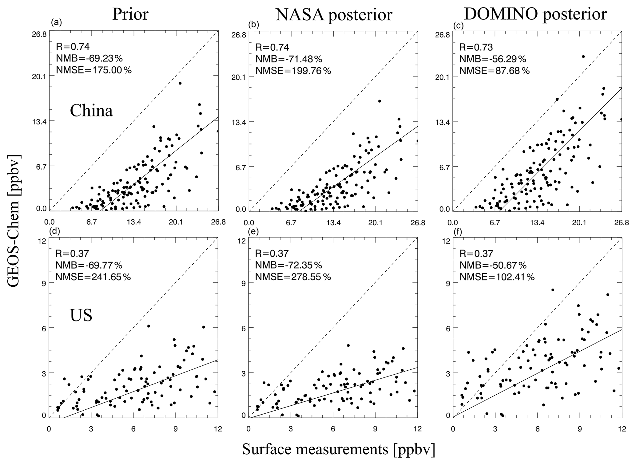
Figure 2Evaluation of annual mean surface NO2 mixing ratios with measurements in China (a, b, c) and the US (d, e, f) in 2015.
Figure 2 shows the comparisons of annual mean surface NO2 concentrations in 2015 from measurements and simulations using different NOx emission inputs. The selection of this year is due to the limited availability of nationwide surface NO2 measurements in China. Surface NO2 concentrations in both China and the US are measured by chemiluminescence analyzers, each equipped with a molybdenum converter, which converts additional NOy compounds to NO and leads to a positive bias in NO2 measurements (Dunlea et al., 2007; Steinbacher et al., 2007). We therefore calculate a correction factor following Lamsal et al. (2008) for each GEOS-Chem simulation and divide the simulated NO2 concentrations by this correction factor to convert simulated NO2 to the measured species. The correction factors are generally higher in the US than in China but have similar seasonality (see Fig. S3 in the Supplement). Subtracting the resolution bias from the statistics shown in Fig. 2, the equivalent normalized mean bias (NMB) of surface NO2 concentrations using the NASA posterior is −54 % in China and −41 % in the US. The equivalent NMB using the DOMINO posterior is −38 % in China and −19 % in the US. These remaining negative biases reflect the unrepresentativeness of 0.1∘ pseudo measurements for real point measurements for resolution bias correction, comparison of NO2 concentrations averaged over simulation to limited measurements, the underestimates of NO2 retrievals using coarse-resolution prior information, and the inability of data assimilation to increase emissions at grid cells where NO2 retrievals are below the detection limit of OMI. Although we have not performed a NOx emission inversion using the QA4ECV product for 2015, we expect its bias to lie between the results from the NASA and DOMINO products, based on the magnitude of NOx emissions in 2010.
We evaluate the simulated ozone concentrations with global surface measurements from the TOAR database using three ozone metrics: maximum daily 8 h average (MDA8) ozone, daytime average ozone (08:00–20:00 LT), and 24 h average ozone. In addition to the GC-adj simulation, with which we derived top-down NOx emissions, we also input the same top-down emissions to GCv12 and evaluate ozone simulations from this more recent version of the GEOS-Chem that includes updated halogen and isoprene chemistry.
All GC-adj simulations of 2 m ozone concentrations have a high bias compared to the TOAR measurements in 2010. NMB and normalized mean square error (NMSE) are largest for 24 h ozone concentrations. Simulations using posterior NOx emissions have slightly better agreement with the measurements from TOAR in 2010 (Fig. 3). In particular, simulations using the DOMINO posterior NOx emissions have the smallest NMB in all ozone metrics and the smallest NMSE in all metrics except for the North Hemisphere (NH) summertime MDA8 ozone. Simulations using the NASA posterior NOx emissions have the best spatial correlation when compared with measurements for all metrics except for the NH summer daytime ozone and annual MDA8 ozone, for which DOMINO posterior simulations have the largest correlation coefficient (Fig. S4).
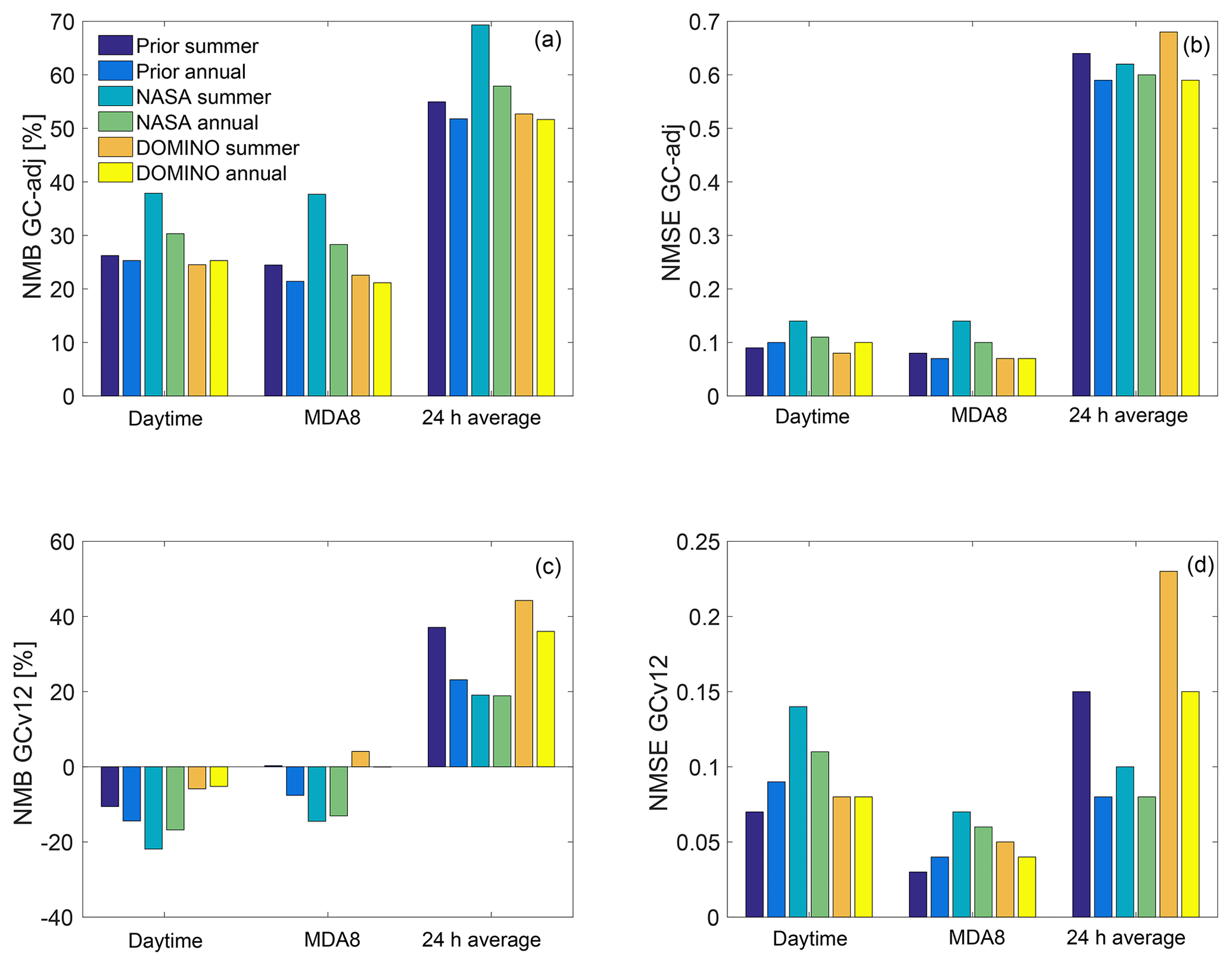
Figure 3NMB and NMSE of annual mean and NH summertime surface ozone concentrations when comparing all measurements from TOAR in 2010 with GC-adj (a, b) and GCv12 (c, d) simulations. The simulations are input with three sets of NOx emissions: CEDS bottom-up inventory (HTAP for GC-adj and CEDS for GCv12), posterior emissions constrained by the NASA product, and posterior emissions constrained by the DOMINO product.
In comparison, GCv12 simulations have a low bias in daytime ozone but high bias in 24 h average ozone, reflecting the potential underestimate of ozone loss at night. The impact of NO2 assimilation on improving estimates of surface ozone simulations in GCv12 depends upon the ozone metric, as shown in Fig. 3c. Simulations using the DOMINO posterior emissions have the smallest NMB for annual mean daytime ozone; simulations using bottom-up NOx emissions have the smallest NMB for annual mean MDA8 ozone; simulations using the NASA posterior emissions have the smallest NMB for annual mean 24 h averaged ozone. These results suggest that the simulated diurnal variations of surface ozone concentrations may not be correct. The current constraints on NOx emissions use observations from OMI, which overpasses the same location approximately once per day. The diurnal variations of NOx emission are constrained to be those of the prior emissions. The daily NO2 column densities from OMI are smaller compared to the diurnally varying ground-based retrievals (Herman et al., 2019). Assimilating NO2 observations from instruments overpassing at different times of the day (e.g., Boersma et al., 2008; Lin et al., 2010; Miyazaki et al., 2017) and using hourly constraints from the geostationary satellite data (e.g., Geo-stationary Environmental Monitoring Spectrometer (GEMS), Tropospheric Emissions: Monitoring of Pollution (TEMPO) (Zoogman et al., 2017), and Sentinel-4) have the potential to improve simulations of ozone diurnal variations and different ozone metrics, although the ratio of NO2 column densities from satellites that overpass in the morning and afternoon are generally lower than the same ratios from surface measurements (Penn and Holloway, 2020). Simulated MDA8 ozone values are mostly biased low in NH summer but biased high in annual mean concentrations, reflecting different seasonal variations in simulated and measured ozone concentrations, which will be further discussed in Sect. 3.2. Evaluations with the CNEMC ozone measurements in China are in Sect. S2 in the Supplement.
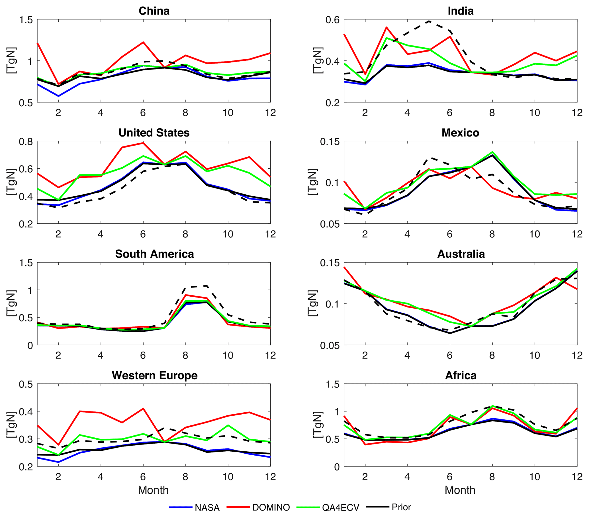
Figure 4Seasonal variations of total 4D-Var posterior NOx emissions in 2010. The black lines are prior emissions from bottom-up inventories (solid lines are from GC-adj; dashed lines are from GCv12). The blue lines are the emissions constrained by the OMI NO2 NASA product. The red lines are emissions constrained by the OMI NO2 DOMINO product. The green lines are emissions constrained by the OMI NO2 QA4ECV product.
3.2 Seasonal variation
The seasonal variations of monthly NOx emissions are consistent between the prior emissions and the NASA posterior emissions (Fig. 4). The DOMINO posterior emissions show different seasonal variations in several regions. In China, the prior emissions and the NASA posterior NOx emissions show summer peaks, which are mainly caused by the increase of natural sources when temperatures are high and lightning occurs more often (Qu et al., 2017). The DOMINO posterior emissions have the largest values in January and June in China, consistent with the posterior seasonality from Miyazaki et al. (2017) constrained by the same OMI NO2 product. The June peak in China has been explained by the crop residual burning (Stavrakou et al., 2016). The peak of the DOMINO posterior NOx emissions in the United States and Mexico shifted earlier in the year to June and July compared to the prior emissions and NASA posterior emissions, similar to the results from Miyazaki et al. (2017). The peak in DOMINO posterior emissions corresponds to the time of high soil NOx emissions, which are reported to be underestimated in high-temperature agricultural systems in the bottom-up inventory (Oikawa et al., 2015; Miyazaki et al., 2017). The differences between the DOMINO posterior and the other two sets of emissions are especially large during the springtime in India, when biomass-burning activity increases (Miyazaki et al., 2017; Venkataraman et al., 2006). These retrieval products have similar numbers of observations and spatial distributions of observation densities after the filtering. The different seasonal variations in the posterior NOx emissions may reflect the AMF structural uncertainties when the retrieved NO2 column densities use different ancillary data (Lorente et al., 2017). For instance, the GEOS-Chem NO2 SCDs converted using the scattering weight from the NASA product have larger seasonal variations than the SCDs converted using the DOMINO scattering weight in the US, reflecting the different seasonal variations of vertical sensitivities from the two retrievals. The seasonal variations of simulated surface NO2 concentrations are similar with measurements in China and the US (see Fig. S6).
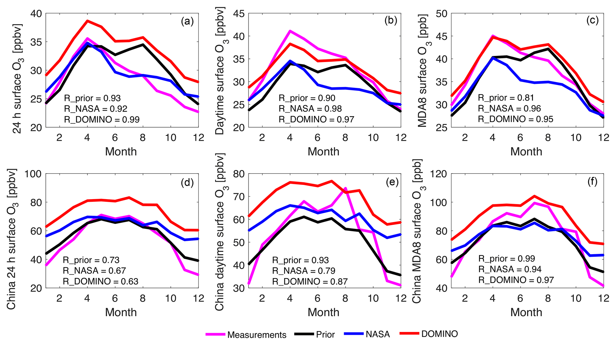
Figure 5Seasonality of surface ozone concentration at 2 m in 2010 compared with TOAR (a, b, c) and in 2015 compared with CNEMC (d, e, f). Surface measurements are shown with magenta lines. Simulations are performed using GCv12 with NOx emissions from CEDS (black line), NASA posterior emissions (blue line), and DOMINO posterior emissions (red line).
Seasonal variations of 2 m ozone concentrations simulated by the GC-adj are also similar despite different NOx emission inputs: the differences in correlation coefficients of the simulated and the measured monthly ozone concentrations are less than 9 %. The simulations of 2 m ozone concentrations from GCv12 show better seasonality when using the posterior NOx emissions than using the prior, as shown in Fig. 5. Simulations using the CEDS inventory show double maxima in April and August, whereas surface measurements only show a single maximum in April. Assimilation of NASA NO2 concentrations alleviates this difference and leads to the largest correlation with measured MDA8 and 24 h average ozone; simulations using the DOMINO posterior emissions have the largest correlation coefficient for daytime ozone. That being said, the correlation coefficients are not notably different. The August ozone peak in the prior simulation is mainly due to the high ozone concentrations in North China, southwest China, and northern India. The NASA and DOMINO posterior simulations have both reduced surface ozone concentrations in the North China Plain and northeast China in August due to the larger posterior NOx emissions than the prior emissions in these high-NOx regions. Both posterior ozone simulations are also smaller than the prior emissions in Tibet and northern India due to the reductions of posterior NOx emissions in low-NOx regions. The August ozone peak in the DOMINO posterior emissions comes from the higher ozone concentrations in Angola and the Democratic Republic of the Congo compared to the NASA posterior and prior simulations in the same month and DOMINO posterior simulations in the previous months. This can be explained by the larger upward adjustment of DOMINO posterior NOx emissions in South Africa in August. These results show the large spatial heterogeneities on the responses of ozone seasonality to the changes in NO2 abundances on a global scale. Compared with CNEMC measurements in China, simulations using the prior emissions have the most consistent seasonal variations and smallest NMSE. All simulations have smaller seasonal variations than the measurements in daytime ozone.
3.3 Interannual variations
The three different versions of NOx emissions have different regional trends from 2005 to 2016 as shown in Fig. 6. In China, the NASA posterior NOx emissions increased by 32 % and the DOMINO posterior NOx emissions increased by 32 % from 2005 to 2011. From 2011 to 2016, they decreased by 20 % (NASA) and 11 % (DOMINO). This turning point reflects the regulation of NOx emissions in China since the “11th 5-year plan” in 2011. In India, both posterior NOx emissions showed continuous increases (by 24 % from the NASA posterior emissions and 34 % from the DOMINO posterior emissions) from 2005 to 2016. The sources of NOx emissions in India are mainly from thermal power and transportation and are expected to continue increasing in the near future under current regulations (Venkataraman et al., 2018). In the US, NOx emissions decreased by 24 % (NASA) and 19 % (DOMINO) from 2005 to 2010 and then flattened from 2010 to 2016. This slowdown in the total top-down NOx emissions was attributed to the growing contribution from industrial, areal, and off-road mobile sources as well as the slower-than-expected decreases in on-road diesel NOx emissions by Jiang et al. (2018). Silvern et al. (2019), however, argued that the slowdown was driven by the weaker decreases in background sources of NOx, which has an increasing contribution with the decrease of anthropogenic NOx sources. In Mexico, the two posterior NOx emissions consistently increased by 6 % (NASA) and 13 % (DOMINO) from 2005 to 2016. The DOMINO posterior emissions show more obvious increase in Mexico from 2010 to 2016. This increase in Mexico is not reflected in the bottom-up estimates from the EPA National Emissions Inventory. In Australia, the NASA posterior emissions increase by 10 % from 2005 to 2016. In comparison, the DOMINO posterior emissions decrease from 2005 to 2010 and increase afterwards, consistent with the posterior emissions trend from Miyazaki et al. (2017). The different trends in posterior NOx emissions are propagated from the trends in the two OMI NO2 retrieval products. The discrepancies are likely due to the different surface albedo and cloud products used in the two retrievals, which affect averaging-kernel sensitivities. The trends of NOx emissions in South America are different in the two posterior estimates after 2012, when the NASA posterior emissions started to decrease by 27 % and the DOMINO posterior emissions started to increase by 11 % up until 2016. In western Europe and Africa, posterior NOx emissions fluctuate and do not have a significant consistent trend from the two inversions.

Figure 6Annual total posterior NOx emissions from 2005 to 2016. The black lines show prior total NOx emissions from bottom-up inventories, which use HTAP anthropogenic emissions in 2010 for all years. The blue lines represent the emissions constrained by the OMI NO2 NASA product. The red lines represent emissions constrained by the OMI NO2 DOMINO product.
The magnitudes of DOMINO posterior NOx emissions are consistently larger than the NASA ones throughout the period. The 12-year averages of annual NOx budgets from NASA posteriors emissions are 37 % (China), 53 % (India), 43 % (US), 50 % (Mexico), 45 % (Australia), 58 % (South America), 47 % (western Europe), and 46 % (Africa) smaller than the DOMINO posterior emissions.
We evaluate the trend of simulated surface NO2 concentrations in the US with AQS measurements due to its availability throughout the study period (Fig. 7). From 2006 to 2016, the surface NO2 concentrations show consistent decreases in the AQS measurements (by 32 %) and GC-adj simulations (by 26 % using the NASA posterior, by 10 % using the DOMINO posterior, and by 7 % using the prior emissions). Since we use the same anthropogenic emissions throughout 2006–2016 in the prior simulations, the variations in the black line reflect changes from natural sources and the impact of meteorological factors (e.g., temperature, humidity, wind, etc.). Surface NO2 simulations using the NASA posterior NOx emissions also have the largest correlation coefficient when compared to the measurements (R2=0.93 for the NASA posterior, R2=0.81 for the DOMINO posterior, and R2=0.74 for the prior). The more consistent trends and correlations in surface NO2 simulations using the NASA posterior emissions are consistent with the larger decrease of NASA posterior NOx emissions in the US (by 20 % or for comparison a decrease of 1 % in the DOMINO posterior) from 2006 to 2016, as shown in Fig. 6.
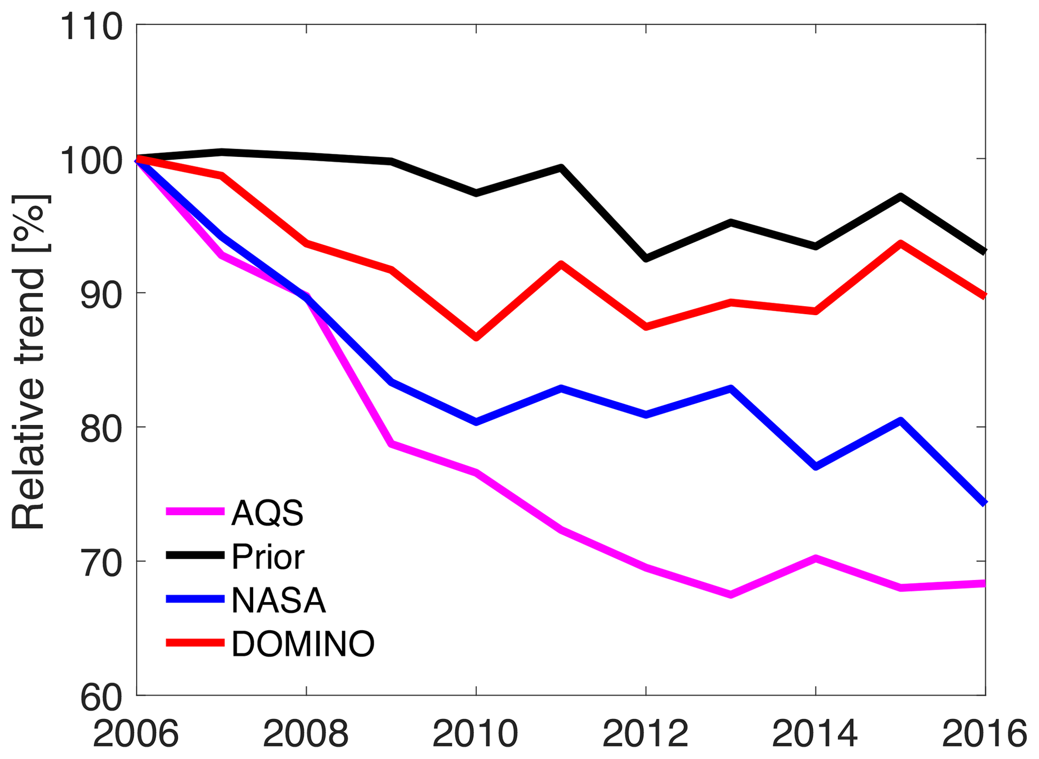
Figure 7The trend of annual mean surface NO2 concentrations over the US from 2006 to 2016, expressed as a percent of the 2006 values. Surface measurements are from EPA AQS sites (magenta line). GEOS-Chem simulations are performed using prior emissions (black line) with constant anthropogenic emissions throughout the years, posterior NOx emissions constrained by the NASA product (blue line), and posterior NOx emissions constrained by the DOMINO product (red line).
The interannual variability of global simulations of 2 m ozone sampled at the TOAR locations is similar between GC-adj and GCv12. During the NH summer, simulations using the DOMINO posterior NOx emissions have the most consistent trend in daytime and 24 h average ozone in both models (see Table S1 in the Supplement); GC-adj simulations using the NASA posterior emissions have the best consistency with the measured trend of MDA8 ozone. The different performances of NOx emission datasets for different ozone metrics is a consequence of the hard constraint on NO2 diurnal variations within the assimilation (and the lack of sufficient observations to constrain this). This can lead to better agreement of mean ozone concentration with measurements over particular hours but worse mean concentrations averaged over other hours. Detailed analyses of global ozone trends are in Sect. S3. At the regional scale, shown in Fig. 8, surface ozone measurements from TOAR mostly fall within the ranges of assimilation results. The interannual variations of simulated ozone over the whole region (black dotted lines) are generally smaller than the ones at grid cells that include surface measurements (solid black lines). The number of years that ozone measurements are available in each grid cell is shown in Fig. S8. The overlap of solid black and green lines in Fig. 8 suggests that interannual variations of anthropogenic NOx emissions from CEDS do not have a large impact on surface ozone simulations. The trends of simulated annual MDA8 ozone concentrations are correlated with impacts from meteorology and non-NOx sources based on simulations (shown as green lines) that use the same anthropogenic NOx emissions for all years and simulations that use interannually varied anthropogenic NOx emissions, leading to ozone changes of up to 4 ppbv (China), 5 ppbv (South Korea), 1 ppbv (US), 2 ppbv (Mexico), 1 ppbv (South America), 1 ppbv (Australia), 1 ppbv (western Europe), and 6 ppbv (Africa) from one year to the next. The trends of simulated MDA8 ozone are similar when using the NASA and the DOMINO posterior NOx emissions as inputs. The DOMINO-derived MDA8 ozone concentrations are higher than the NASA-derived ones in all studied regions, represented by the upper and lower limits of the error bars, respectively. GCv12 simulated ozone concentrations are smaller than simulations from GC-adj, especially over relatively less polluted regions, consistent with the inclusion of halogen chemistry in GCv12, which depleted ozone. The simulated MDA8 ozone trends in grid cells that include measurements in the US and Australia are more consistent with the TOAR measurements than the other regions, with coefficients of determination (R2) larger than 0.45. The larger differences in ozone between the prior and posterior emissions as well as variability between the two top-down NOx emissions in GCv12 suggest a larger responsiveness of the ozone chemistry to changes in NOx. We do not expect simulated ozone trends to be completely consistent with the measurements in the TOAR database due to errors in the model's transport, chemical mechanism, and VOC emissions.
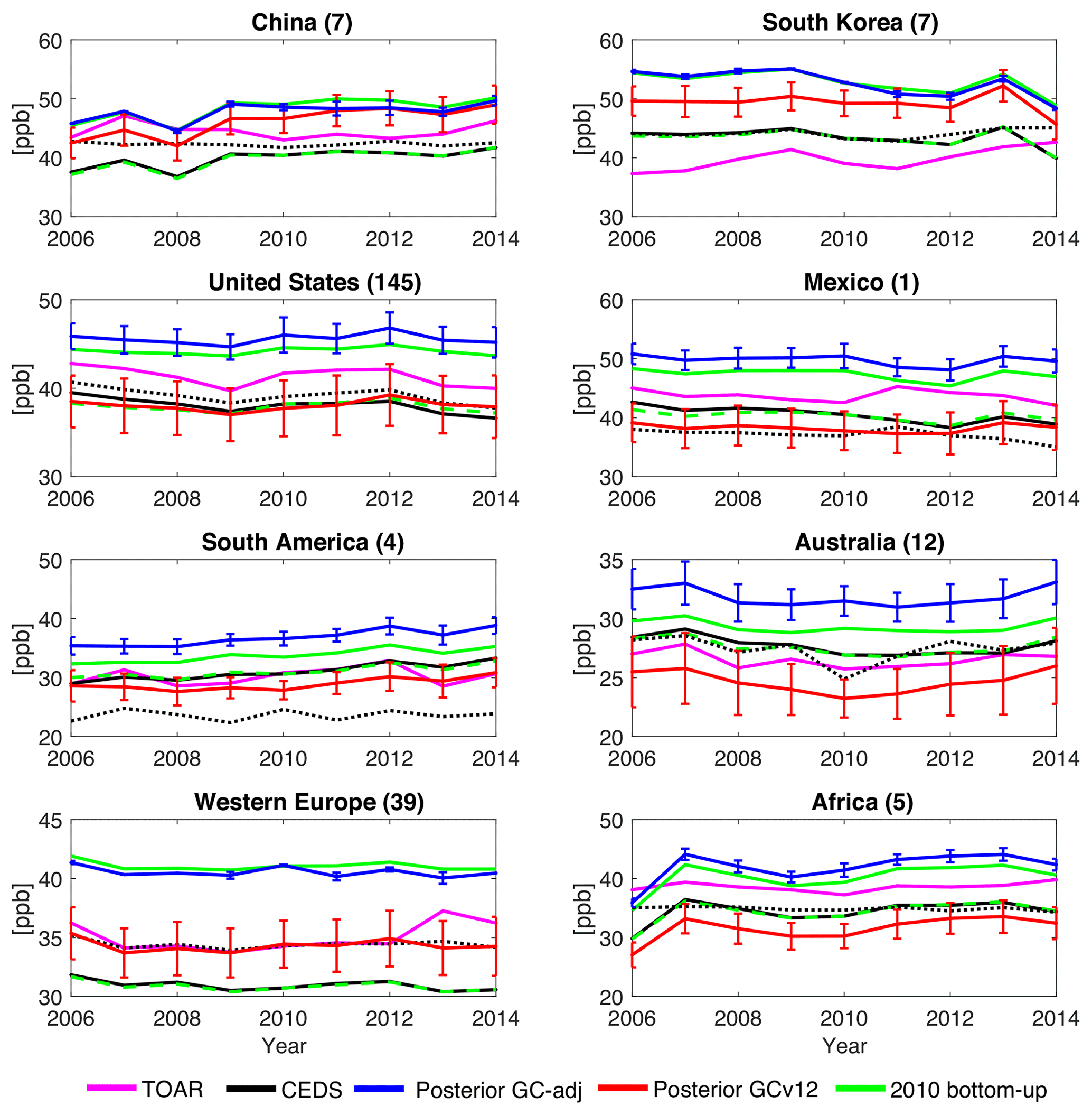
Figure 8The trends of regional mean annual MDA8 ozone concentrations from 2006 to 2014. Surface measurements are from the TOAR database (magenta line). Only sites that have continuous measurements throughout the 9 years are included. The numbers in the parenthesis are the number of grid cells that include monitoring sites in each region. The black dotted lines show the national mean of surface ozone from GCv12 simulations using the CEDS inventory. The other lines are simulations from GC-adj and GCv12 averaged over the grid cells that include monitoring sites. Black lines show ozone simulations using the bottom-up NOx emissions from CEDS in each corresponding year. Green lines show ozone simulations using 2010 bottom-up NOx emissions for all years (HTAP 2010 for GC-adj shown in solid lines, CEDS 2010 for GCv12 shown in dashed lines). The vertical bars represent the spread of simulated surface ozone concentrations using the NASA and the DOMINO posterior NOx emissions.
We further separate the ozone trends in grid cells that include measurements into changes caused by NOx emissions as well as meteorology and non-NOx sources. The second trend is calculated through simulations that use constant NOx emissions throughout the studied years. It has a similar trend from GCv12 and GC-adj as shown in the green lines in Fig. 9. The trend caused by NOx emissions is obtained by subtracting the second trend from the ozone trend simulated using NOx emissions at each corresponding year. The ozone trends due to changes in meteorology and non-NOx sources (green lines) are moderately correlated (R>0.5) with measurements from TOAR in Australia, the US, South America, and India. The ozone trends due to changes in posterior NOx emissions (red and blue lines) only have positive correlations with TOAR measurements in both GC-adj and GCv12 simulations in Africa and Australia. Ozone measurements in 2014 decreased compared to the 2006 level in the US and Mexico. GC-adj simulations do not have significant trends in these regions, whereas GC-v12 simulations show increases in China, the US, and Mexico. Meteorological and non-NOx sources lead to larger interannual variations in ozone simulations than those driven by NOx emissions in South America, Australia, and Africa, where anthropogenic activities are much less than the other regions. These underscore the challenges of attributing observed variations in ozone to changes in NOx emissions at regional scales.
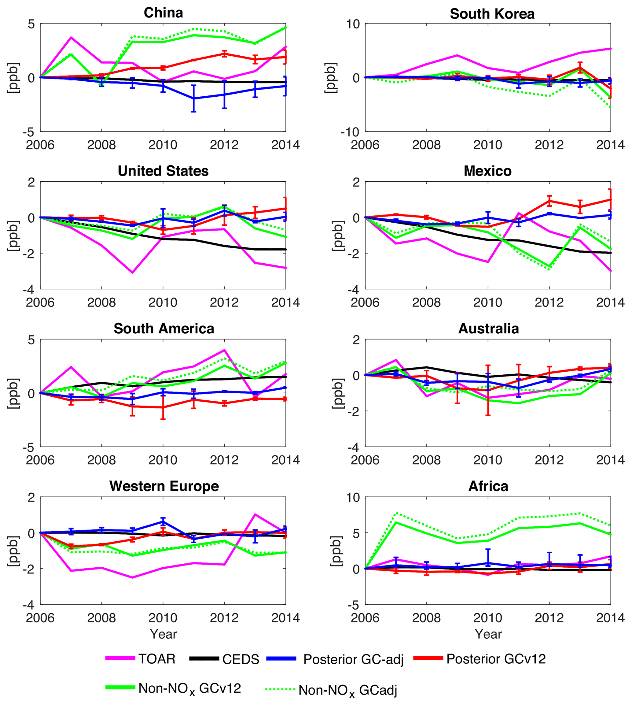
Figure 9Changes of regional mean annual MDA8 ozone concentrations compared to 2006 from TOAR measurements (magenta line), due to changes in bottom-up NOx emissions (black), due to changes in top-down NOx emissions (blue lines for simulations from GC-adj and red lines for simulations from GCv12), and due to changes in meteorology and non-NOx emissions (green lines). Only sites that have continuous measurements throughout the 9 years are included. The vertical bars represent the spread of changes from simulations using the NASA and the DOMINO posterior NOx emissions. The impacts of meteorology and natural sources are removed from black, blue, and red lines by subtracting simulations using 2010 bottom-up anthropogenic emissions for all years from simulations that use bottom-up NOx emissions corresponding to each year.
Assimilations of ozone precursor gases have the potential to improve remote-ozone simulations, which can be used to provide boundary conditions for regional air quality models and to quantify and attribute sources of background ozone. We therefore focus specifically on remote regions in the US in this section to evaluate the vertical profile and surface concentrations of ozone simulations.
4.1 Evaluations with ozonesonde profiles
Field campaigns and routine observations of ozone concentrations along the west coast of the US have provided opportunities to understand regional and intercontinental influences on surface air quality (Cooper et al., 2015). Evaluations with the IONS-2010 measurements in Fig. 10 show that the GCv12 simulations of ozone vertical profiles have negative biases (NMB between −8 % and −32 %) above all six sites. The standard deviations of ozonesonde and simulated profiles overlap with each other (see Fig. S9). The GC-adj simulations have positive biases at San Nicolas and Trinidad Head and have smaller negative biases (NMB between −3 % and −11 %) at the remaining sites than the GCv12 simulations. The magnitudes of the NMSE and NMB of the GCv12 simulations at 700–900 hPa are also larger than those of the GC-adj simulations (see Fig. S10). The prior simulations in GCv12 apply NOx emissions at different altitudes, whereas the posterior GCv12 and all GC-adj simulations apply all NOx emissions to the surface. This leads to different transport and formation of ozone at different model layers and therefore causes larger differences in ozone simulations in the upper troposphere. The air masses at this altitude in the eastern Pacific are demonstrated to impact inland near-surface ozone concentrations (Cooper et al., 2011; Lin et al., 2012; Yates et al., 2015). The different biases in ozone simulations close to the surface can be explained by the usage of different emission inventories (e.g., different biogenic emissions) and different boundary layer mixing schemes (nonlocal mixing (Lin and McElroy, 2010) in GCv12 and full mixing in GC-adj). The different chemical mechanisms in the two model versions affect the different model biases especially in the upper troposphere. For instance, inclusion of halogen chemistry and additional chlorine chemistry in GCv12 leads to 19 % and 7 % decreases of global tropospheric ozone burden (Sherwen et al., 2016a; Wang et al., 2019). GCv12 simulations using the CEDS emissions have smaller NMSE and NMB than the simulations using the posterior NOx emissions in all six sites in 2010. In comparison, the GC-adj simulations using the DOMINO posterior NOx emissions have the smallest NMSE and NMB at all sites except for San Nicolas and Trinidad Head, where the prior simulations have the smallest error and bias. Further evaluations with ozonesondes at Trinidad Head in 2016 are shown in Sect. S4 in the Supplement.
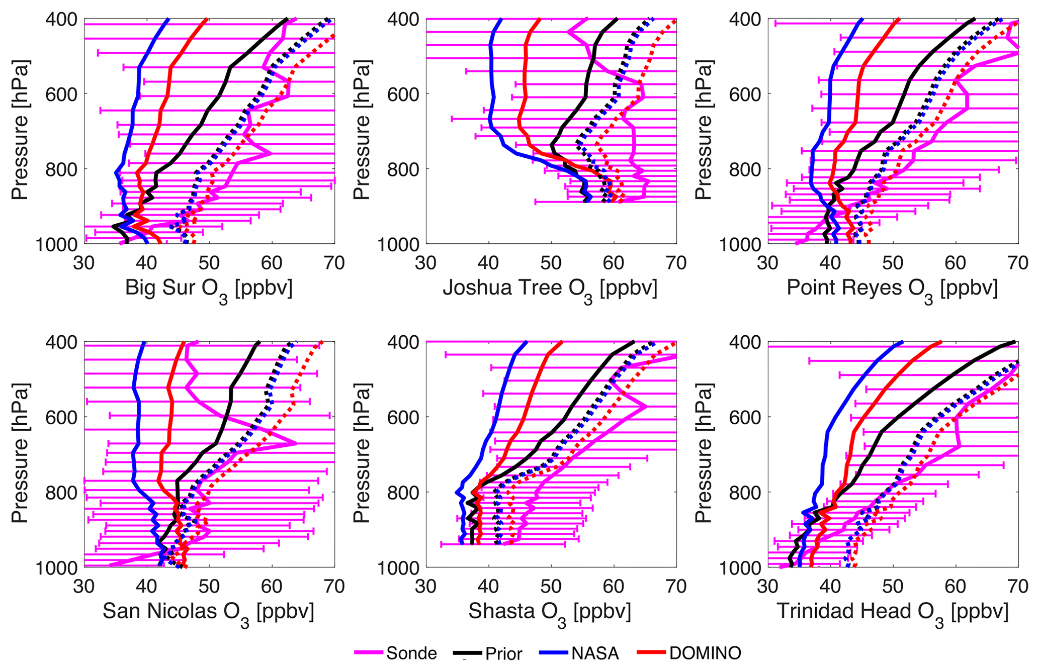
Figure 10Ozone vertical profiles averaged over May and June 2010 from six ozonesonde measurement sites from the IONS-2010 field experiment in California. The six sites are over remote regions and are used to evaluate the intercontinental transport of ozone. Solid black (prior emissions), blue (NASA posterior emissions), and red (DOMINO posterior emissions) lines are from the GCv12 simulations (prior anthropogenic emissions from CEDS), whereas dashed lines are from the GC-adj simulations (prior anthropogenic emissions from HTAP). The horizontal bars show the standard deviations of the measurements at each vertical layer.
4.2 Evaluations with TOAR surface ozone measurements at remote sites
To further evaluate the model performance under different geographical scenarios, we compare surface ozone simulations from GC-adj and GCv12 with observations from simple to complex environments. These include (1) Mauna Loa Observatory and Mt. Bachelor Observatory at night, which represent the lower free troposphere, and (2) Mt. Bachelor Observatory, Lassen Volcanic National Park, Great Basin National Park, and Sequoia/Kings Canyon National Park at daytime, representing high-elevation rural sites during well-mixed daytime conditions. The coefficients of determination (see Table S2) between the simulations and the measurements are larger than 0.6 for all daytime ozone comparisons except for Mt. Bachelor Observatory. The correlation coefficients are smaller than 0.5 for all nighttime comparisons, reflecting the need to further improve simulations of nighttime chemistry and atmospheric processes.
In Fig. 11, the surface ozone concentrations from both GC-adj and GCv12 simulations have low biases compared to the surface measurements at remote sites. These low biases in the GCv12 simulations are consistent with its performances when evaluated with ozonesondes from IONS-2010 and with daytime surface ozone at the global scale. However, the low biases in the GC-adj simulations are different from its high biases when compared with the global surface ozone concentrations and the ozone profiles at San Nicolas and Trinidad Head. This demonstrates the different biases in ozone simulations at rural and urban sites. Simulations using the DOMINO posterior emissions have the smallest NMSE and NMB at all remote sites except for the GCv12 simulations at Mauna Loa at night and Great Basin National Park during the daytime.
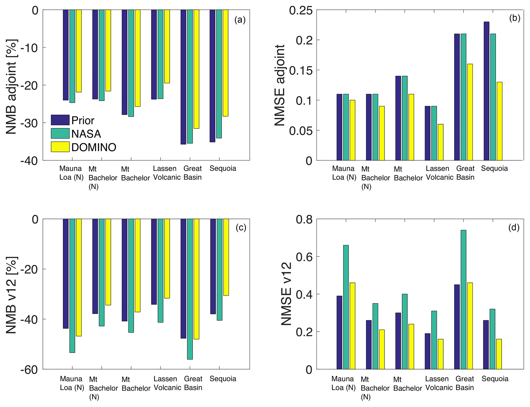
Figure 11NMSE and NMB of GC-adj (a, b) and GCv12 (c, d) ozone simulations in 2010–2014 evaluated with surface measurements at remote sites. Three sets of NOx emissions, i.e., bottom-up inventory (HTAP for GC-adj, CEDS for GCv12), DOMINO posterior emissions, and NASA posterior emissions, are input in each model. Site names with “(N)” represent nighttime. The rest are comparisons at daytime.
We performed global inversions of NOx emissions from 2005 to 2016 using two widely used OMI NO2 retrievals from NASA (OMNO2 v3) and KNMI (DOMINO v2). Different vertical sensitivities from the two retrievals are a major cause of the discrepancies in the posterior emissions. The DOMINO posterior NOx emissions have a larger magnitude than the prior emissions and the NASA posterior emissions. Consequently, GC-adj simulations using the DOMINO posterior NOx emissions have the smallest negative bias in surface NO2 and the smallest positive bias in 2 m ozone. The impact of NO2 assimilations on improving estimates of the GCv12 surface ozone simulations depends upon the ozone metrics, suggesting inaccurate diurnal variations in the surface ozone simulations. GEOS-Chem simulations using the DOMINO posterior emissions have the largest coefficients of determination for summertime daytime (R2=0.81) and summertime 24 h (R2=0.96) ozone. Simulations using the NASA posterior emissions have the smallest bias and error for all ozone metrics and the largest correlation for summertime MDA8 ozone (R2=0.88). Ozone simulations with GEOS-Chem v12.1.1 using the DOMINO posterior NOx emissions lead to the most consistent seasonality in 24 h average ozone (R2=0.99) with TOAR measurements, while the NASA posterior emissions lead to the best agreement in seasonal variations of MDA8 (R=0.96) and daytime ozone (R=0.98). The interannual variations of posterior NOx emissions from the two products are similar in China, India, the US, Mexico, and Australia but different in South America, western Europe, and Africa. Surface NO2 simulations using the NASA posterior emissions have the best agreement with measurements in the US. Daytime and 24 h average ozone simulations using the DOMINO posterior also have the best trend (R=0.72 and 0.88) in the Northern Hemisphere summer. The GC-adj simulations using the NASA posterior NOx emissions have the best trend in MDA8 ozone in NH summer.
Posterior NOx emissions lead to improved simulations of ozone at several remote sites in the western US. The GC-adj simulations using the DOMINO posterior emissions have the smallest NMSE and NMB compared to ozonesonde measurements during IONS-2010, except for the San Nicolas and Trinidad Head sites. At the remote surface sites evaluated in this study, surface ozone simulations using the DOMINO posterior emissions have the best performance except for GCv12 simulations at Mauna Loa at night and Great Basin National Park during the daytime. The reduced negative biases in daytime surface ozone simulations using the DOMINO posterior emissions at these remote sites and at most IONS-2010 sites are consistent with the increases of daytime remote ozone in the western US through NO2 and ozone data assimilation in Huang et al. (2015). Simulations using the DOMINO posterior emissions are demonstrated to provide more precise magnitudes at these remote sites and can potentially be used as boundary conditions for regional air quality models for further air pollution and health studies.
The remaining differences between simulated and measured ozone can be explained by the roles of VOCs, errors in satellite retrievals, and uncertainties in the chemical and physical processes in the model simulations. In addition to NOx, emissions of other ozone precursors also impact the accuracy of ozone simulations. For instance, inversion of isoprene emissions over the southeast US decreases surface ozone simulations by 1–3 ppbv (Kaiser et al., 2018). Inversion of non-methane VOC emissions changes surface afternoon ozone simulations by up to 10 ppbv in China (Cao et al., 2018). Assimilation of multiple species (e.g., ozone, CO, HNO3, and SO2) together with NO2 may improve posterior ozone simulations, but the performance of posterior simulations may depend on the chemical transport model, as shown in Miyazaki et al. (2020), where the GEOS-Chem adjoint model v35 shows mixed performance in correcting the bias between ozonesonde and posterior simulations between 850 and 500 hPa at different latitude bands. Both OMI NO2 retrievals employed in this study use NO2 vertical shape factors from coarse-resolution simulations and therefore are biased low compared to in situ measurements (Goldberg et al., 2017). These retrievals also have not explicitly accounted for the aerosol optical effects, which are demonstrated to degrade the accuracy of NO2 column concentrations when aerosol optical depth (AOD) is very high (Chimot et al., 2016; Liu et al., 2019; Cooper et al., 2019). The differences in the magnitude of ozone concentrations from GC-adj and GCv12 reflect the impact of other species emissions and chemical mechanisms on the bias of ozone simulations. Previous studies also show that global simulations at coarse resolution are not able to capture the observed persistence of chemical plumes in the free troposphere on intercontinental scales, leading therefore to underestimates of remote-ozone concentrations (Hudman et al., 2004; Zhuang et al., 2018).
Although biases, errors, seasonalities, and interannual variations of ozone simulations have been improved in several cases through constraints on NOx emissions, there are still large discrepancies in the vertical profile and diurnal variations between ozone simulations and measurements. For instance, the different performances of each set of NOx emissions on the simulations of different ozone metrics reflect errors in the ozone diurnal simulations. The differences in ozone vertical profiles suggest errors in vertical transport in the model. These discrepancies could not be improved by adjusting only surface NOx emissions using observations at one time of the day, as performed in this study. Future geostationary satellite observations will provide opportunities to update NOx emissions at every hour. Separately constraining NOx emissions from the surface (e.g., anthropogenic sources) and the upper atmosphere (e.g., lightning sources, Pickering et al., 2016) as well as implementing these posterior NOx emissions at their corresponding vertical levels can potentially improve the vertical profile of ozone simulations.
Top-down NOx emissions derived in this work can be downloaded from https://dataverse.harvard.edu/dataverse/zhenqu (last access: 1 November 2020, Qu et al., 2020a, b). The OMI NO2 NASA standard product is downloaded from GES DISC (https://atrain.gesdisc.eosdis.nasa.gov/data/OMI/OMNO_CPR.003/, last access: 1 November 2020, NASA, 2020). The DOMINO and QA4ECV NO2 retrievals are from KNMI (http://www.temis.nl/airpollution/no2.html, last access: 1 November 2020). Ozonesonde profiles from Shasta, Big Sur, Point Reyes, Joshua Tree, and San Nicolas are available from the NOAA Global Monitoring Laboratory (ftp://aftp.cmdl.noaa.gov/data/ozwv/Ozonesonde/2_Field Projects/CALNEX/, last access: 1 November 2020, NOAA, 2020a); Ozonesondes from Trinidad Head are also available from the NOAA Global Monitoring Laboratory (ftp://aftp.cmdl.noaa.gov/data/ozwv/Ozonesonde/Trinidad Head, California/100 Meter Average Files/, last access: 1 November 2020, NOAA, 2020b). Pre-compiled TOAR ozone data were downloaded from https://doi.org/10.1594/PANGAEA.876108 (Schultz et al., 2017b).
The supplement related to this article is available online at: https://doi.org/10.5194/acp-20-13109-2020-supplement.
ZQ, DKH, ORC, and JLN designed the research; ZQ performed the research and prepared the paper with help from all authors.
The authors declare that they have no conflict of interest.
Part of the computing resources supporting this work was provided by the NASA High-End Computing (HEC) program through the NASA Advanced Supercomputing (NAS) division at Ames Research Center. Zhen Qu would also like to acknowledge high-performance computing support from Cheyenne (https://doi.org/10.5065/D6RX99HX, NCAR, 2020) provided by NCAR's Computational and Information Systems Laboratory, sponsored by the National Science Foundation.
This research has been supported by the National Aeronautics and Space Administration (grant nos. HAQAST NNX16AQ26G and ACMAP NNX17AF63G).
This paper was edited by Robert Harley and reviewed by two anonymous referees.
Bell, N., Hsu, L., Jacob, D. J., Schultz, M. G., Blake, D. R., Butler, J. H., King, D. B., Lobert, J. M., and Maier-Reimer, E.: Methyl iodide: Atmospheric budget and use as a tracer of marine convection in global models, J. Geophys. Res.-Atmos., 107, ACH 8–1–ACH 8–12, https://doi.org/10.1029/2001JD001151, 2002.
Boersma, K. F., Jacob, D. J., Bucsela, E. J., Perring, A. E., Dirksen, R., van der A, R. J., Yantosca, R. M., Park, R. J., Wenig, M. O., and Bertram, T. H.: Validation of OMI tropospheric NO2 observations during INTEX-B and application to constrain NOx emissions over the eastern United States and Mexico, Atmos. Environ., 42, 4480–4497, https://doi.org/10.1016/j.atmosenv.2008.02.004, 2008.
Boersma, K. F., Eskes, H. J., Dirksen, R. J., van der A, R. J., Veefkind, J. P., Stammes, P., Huijnen, V., Kleipool, Q. L., Sneep, M., Claas, J., Leitão, J., Richter, A., Zhou, Y., and Brunner, D.: An improved tropospheric NO2 column retrieval algorithm for the Ozone Monitoring Instrument, Atmos. Meas. Tech., 4, 1905–1928, https://doi.org/10.5194/amt-4-1905-2011, 2011.
Boersma, K. F., Eskes, H. J., Richter, A., De Smedt, I., Lorente, A., Beirle, S., van Geffen, J. H. G. M., Zara, M., Peters, E., Van Roozendael, M., Wagner, T., Maasakkers, J. D., van der A, R. J., Nightingale, J., De Rudder, A., Irie, H., Pinardi, G., Lambert, J.-C., and Compernolle, S. C.: Improving algorithms and uncertainty estimates for satellite NO2 retrievals: results from the quality assurance for the essential climate variables (QA4ECV) project, Atmos. Meas. Tech., 11, 6651–6678, https://doi.org/10.5194/amt-11-6651-2018, 2018.
Byrd, R. H., Lu, P., Nocedal, J., and Zhu, C.: A Limited memory algorithm for bound constrained optimization, SIAM J. Sci. Comput., 16, 1190–1208, https://doi.org/10.1137/0916069, 1995.
Canty, T. P., Hembeck, L., Vinciguerra, T. P., Anderson, D. C., Goldberg, D. L., Carpenter, S. F., Allen, D. J., Loughner, C. P., Salawitch, R. J., and Dickerson, R. R.: Ozone and NOx chemistry in the eastern US: evaluation of CMAQ/CB05 with satellite (OMI) data, Atmos. Chem. Phys., 15, 10965–10982, https://doi.org/10.5194/acp-15-10965-2015, 2015.
Cao, H., Fu, T.-M., Zhang, L., Henze, D. K., Miller, C. C., Lerot, C., Abad, G. G., De Smedt, I., Zhang, Q., van Roozendael, M., Hendrick, F., Chance, K., Li, J., Zheng, J., and Zhao, Y.: Adjoint inversion of Chinese non-methane volatile organic compound emissions using space-based observations of formaldehyde and glyoxal, Atmos. Chem. Phys., 18, 15017–15046, https://doi.org/10.5194/acp-18-15017-2018, 2018.
Chance, K. and Martin, R. V.: Spectroscopy and Radiative Transfer of Planetary Atmospheres, Oxford University Press, 2017.
Chan Miller, C., Jacob, D. J., Marais, E. A., Yu, K., Travis, K. R., Kim, P. S., Fisher, J. A., Zhu, L., Wolfe, G. M., Hanisco, T. F., Keutsch, F. N., Kaiser, J., Min, K.-E., Brown, S. S., Washenfelder, R. A., González Abad, G., and Chance, K.: Glyoxal yield from isoprene oxidation and relation to formaldehyde: chemical mechanism, constraints from SENEX aircraft observations, and interpretation of OMI satellite data, Atmos. Chem. Phys., 17, 8725–8738, https://doi.org/10.5194/acp-17-8725-2017, 2017.
Chimot, J., Vlemmix, T., Veefkind, J. P., de Haan, J. F., and Levelt, P. F.: Impact of aerosols on the OMI tropospheric NO2 retrievals over industrialized regions: how accurate is the aerosol correction of cloud-free scenes via a simple cloud model?, Atmos. Meas. Tech., 9, 359–382, https://doi.org/10.5194/amt-9-359-2016, 2016.
Cooper, M. J., Martin, R. V., Hammer, M. S., and McLinden, C. A.: An Observation-Based Correction for Aerosol Effects on Nitrogen Dioxide Column Retrievals Using the Absorbing Aerosol Index, Geophys. Res. Lett., 46, 8442–8452, https://doi.org/10.1029/2019GL083673, 2019.
Cooper, O. R., Trainer, M., Thompson, A. M., Oltmans, S. J., Tarasick, D. W., Witte, J. C., Stohl, A., Eckhardt, S., Lelieveld, J., Newchurch, M. J., Johnson, B. J., Portmann, R. W., Kalnajs, L., Dubey, M. K., Leblanc, T., McDermid, I. S., Forbes, G., Wolfe, D., Carey-Smith, T., Morris, G. A., Lefer, B., Rappenglück, B., Joseph, E., Schmidlin, F., Meagher, J., Fehsenfeld, F. C., Keating, T. J., Van Curen, R. A., and Minschwaner, K.: Evidence for a recurring eastern North America upper tropospheric ozone maximum during summer, J. Geophys. Res.-Atmos., 112, D23304, https://doi.org/10.1029/2007jd008710, 2007.
Cooper, O. R., Oltmans, S. J., Johnson, B. J., Brioude, J., Angevine, W., Trainer, M., Parrish, D. D., Ryerson, T. R., Pollack, I., Cullis, P. D., Ives, M. A., Tarasick, D. W., Al-Saadi, J., and Stajner, I.: Measurement of western U.S. baseline ozone from the surface to the tropopause and assessment of downwind impact regions, J. Geophys. Res.-Atmos., 116, https://doi.org/10.1029/2011jd016095, 2011.
Cooper, O. R., Langford, A. O., Parrish, D. D., and Fahey, D. W.: Challenges of a lowered U.S. ozone standard, Science, 348, 1096–1097, https://doi.org/10.1126/science.aaa5748, 2015.
Crutzen, P.: A discussion of the chemistry of some minor constituents in the stratosphere and troposphere, Pure Appl. Geophys., 106, 1385–1399, 1973.
Derwent, R. G., Jenkin, M. E., and Saunders, S. M.: Photochemical ozone creation potentials for a large number of reactive hydrocarbons under European conditions, Atmos. Environ., 30, 181–199, 1996.
Dunlea, E. J., Herndon, S. C., Nelson, D. D., Volkamer, R. M., San Martini, F., Sheehy, P. M., Zahniser, M. S., Shorter, J. H., Wormhoudt, J. C., Lamb, B. K., Allwine, E. J., Gaffney, J. S., Marley, N. A., Grutter, M., Marquez, C., Blanco, S., Cardenas, B., Retama, A., Ramos Villegas, C. R., Kolb, C. E., Molina, L. T., and Molina, M. J.: Evaluation of nitrogen dioxide chemiluminescence monitors in a polluted urban environment, Atmos. Chem. Phys., 7, 2691–2704, https://doi.org/10.5194/acp-7-2691-2007, 2007.
Eastham, S. D., Weisenstein, D. K., and Barrett, S. R. H.: Development and evaluation of the unified tropospheric–stratospheric chemistry extension (UCX) for the global chemistry-transport model GEOS-Chem, Atmos. Environ., 89, 52–63, 2014.
Fiore, A. M., Oberman, J. T., Lin, M. Y., Zhang, L., Clifton, O. E., Jacob, D. J., Naik, V., Horowitz, L. W., Pinto, J. P., and Milly, G. P.: Estimating North American background ozone in U.S. surface air with two independent global models: Variability, uncertainties, and recommendations, Atmos. Environ., 96, 284–300, 2014.
Fisher, J. A., Jacob, D. J., Travis, K. R., Kim, P. S., Marais, E. A., Chan Miller, C., Yu, K., Zhu, L., Yantosca, R. M., Sulprizio, M. P., Mao, J., Wennberg, P. O., Crounse, J. D., Teng, A. P., Nguyen, T. B., St. Clair, J. M., Cohen, R. C., Romer, P., Nault, B. A., Wooldridge, P. J., Jimenez, J. L., Campuzano-Jost, P., Day, D. A., Hu, W., Shepson, P. B., Xiong, F., Blake, D. R., Goldstein, A. H., Misztal, P. K., Hanisco, T. F., Wolfe, G. M., Ryerson, T. B., Wisthaler, A., and Mikoviny, T.: Organic nitrate chemistry and its implications for nitrogen budgets in an isoprene- and monoterpene-rich atmosphere: constraints from aircraft (SEAC4RS) and ground-based (SOAS) observations in the Southeast US, Atmos. Chem. Phys., 16, 5969–5991, https://doi.org/10.5194/acp-16-5969-2016, 2016.
Fleming, Z. L., Doherty, R. M., von Schneidemesser, E., Malley, C. S., Cooper, O. R., Pinto, J. P., Colette, A., Xu, X., Simpson, D., Schultz, M. G., Lefohn, A. S., Hamad, S., Moolla, R., Solberg, S., and Feng, Z.: Tropospheric Ozone Assessment Report: Present-day ozone distribution and trends relevant to human health, Elem. Sci. Anth., 6, 12, https://doi.org/10.1525/elementa.273, 2018.
Fowler, D., Pilegaard, K., Sutton, M. A., Ambus, P., Raivonen, M., Duyzer, J., Simpson, D., Fagerli, H., Fuzzi, S., Schjoerring, J. K., Granier, C., Neftel, A., Isaksen, I. S. A., Laj, P., Maione, M., Monks, P. S., Burkhardt, J., Daemmgen, U., Neirynck, J., Personne, E., Wichink-Kruit, R., Butterbach-Bahl, K., Flechard, C., Tuovinen, J. P., Coyle, M., Gerosa, G., Loubet, B., Altimir, N., Gruenhage, L., Ammann, C., Cieslik, S., Paoletti, E., Mikkelsen, T. N., Ro-Poulsen, H., Cellier, P., Cape, J. N., Horváth, L., Loreto, F., Niinemets, Ü., Palmer, P. I., Rinne, J., Misztal, P., Nemitz, E., Nilsson, D., Pryor, S., Gallagher, M. W., Vesala, T., Skiba, U., Brüggemann, N., Zechmeister-Boltenstern, S., Williams, J., O'Dowd, C., Facchini, M. C., de Leeuw, G., Flossman, A., Chaumerliac, N., and Erisman, J. W.: Atmospheric composition change: Ecosystems–Atmosphere interactions, Atmos. Environ., 43, 5193–5267, https://doi.org/10.1016/j.atmosenv.2009.07.068, 2009.
Gaudel, A., Cooper, O. R., Ancellet, G., Barret, B., Boynard, A., Burrows, J. P., Clerbaux, C., Coheur, P.-F., Cuesta, J., Cuevas, E., Doniki, S., Dufour, G., Ebojie, F., Foret, G., Garcia, O., Granados Muños, M. J., Hannigan, J. W., Hase, F., Huang, G., Hassler, B., Hurtmans, D., Jaffe, D., Jones, N., Kalabokas, P., Kerridge, B., Kulawik, S. S., Latter, B., Leblanc, T., Le Flochmoën, E., Lin, W., Liu, J., Liu, X., Mahieu, E., McClure-Begley, A., Neu, J. L., Osman, M., Palm, M., Petetin, H., Petropavlovskikh, I., Querel, R., Rahpoe, N., Rozanov, A., Schultz, M. G., Schwab, J., Siddans, R., Smale, D., Steinbacher, M., Tanimoto, H., Tarasick, D. W., Thouret, V., Thompson, A. M., Trickl, T., Weatherhead, E., Wespes, C., Worden, H. M., Vigouroux, C., Xu, X., Zeng, G., and Ziemke, J.: Tropospheric Ozone Assessment Report: Present-day distribution and trends of tropospheric ozone relevant to climate and global atmospheric chemistry model evaluation, Elem. Sci. Anth., 6, 39, https://doi.org/10.1525/elementa.291, 2018.
Goldberg, D. L., Lamsal, L. N., Loughner, C. P., Swartz, W. H., Lu, Z., and Streets, D. G.: A high-resolution and observationally constrained OMI NO2 satellite retrieval, Atmos. Chem. Phys., 17, 11403–11421, https://doi.org/10.5194/acp-17-11403-2017, 2017.
Goldstein, A. H., Millet, D. B., McKay, M., Jaegle, L., Horowitz, L., Cooper, O., Hudman, R., Jacob, D. J., Oltmans, S., and Clarke, A.: Impact of Asian emissions on observations at Trinidad Head, California, during ITCT 2K2, J. Geophys. Res.-Atmos., 109, D23S17, https://doi.org/10.1029/2003JD004406, 2004.
Henze, D. K., Hakami, A., and Seinfeld, J. H.: Development of the adjoint of GEOS-Chem, Atmos. Chem. Phys., 7, 2413–2433, https://doi.org/10.5194/acp-7-2413-2007, 2007.
Henze, D. K., Seinfeld, J. H., and Shindell, D. T.: Inverse modeling and mapping US air quality influences of inorganic PM2.5 precursor emissions using the adjoint of GEOS-Chem, Atmos. Chem. Phys., 9, 5877–5903, https://doi.org/10.5194/acp-9-5877-2009, 2009.
Herman, J., Abuhassan, N., Kim, J., Kim, J., Dubey, M., Raponi, M., and Tzortziou, M.: Underestimation of column NO2 amounts from the OMI satellite compared to diurnally varying ground-based retrievals from multiple PANDORA spectrometer instruments, Atmos. Meas. Tech., 12, 5593–5612, https://doi.org/10.5194/amt-12-5593-2019, 2019.
Hoesly, R. M., Smith, S. J., Feng, L., Klimont, Z., Janssens-Maenhout, G., Pitkanen, T., Seibert, J. J., Vu, L., Andres, R. J., Bolt, R. M., Bond, T. C., Dawidowski, L., Kholod, N., Kurokawa, J.-I., Li, M., Liu, L., Lu, Z., Moura, M. C. P., O'Rourke, P. R., and Zhang, Q.: Historical (1750–2014) anthropogenic emissions of reactive gases and aerosols from the Community Emissions Data System (CEDS), Geosci. Model Dev., 11, 369–408, https://doi.org/10.5194/gmd-11-369-2018, 2018.
Hsu, J. and Prather, M. J.: Stratospheric variability and tropospheric ozone, J. Geophys. Res.-Atmos., 114, D06102, https://doi.org/10.1029/2008JD010942, 2009.
Huang, M., Bowman, K. W., Carmichael, G. R., Lee, M., Chai, T., Spak, S. N., Henze, D. K., Darmenov, A. S., and da Silva, A. M.: Improved western U.S. background ozone estimates via constraining nonlocal and local source contributions using Aura TES and OMI observations, J. Geophys. Res.-Atmos., 120, 3572–3592, https://doi.org/10.1002/2014JD022993, 2015.
Hudman, R. C., Jacob, D. J., Cooper, O. R., Evans, M. J., Heald, C. L., Park, R. J., Fehsenfeld, F., Flocke, F., Holloway, J., Hübler, G., Kita, K., Koike, M., Kondo, Y., Neuman, A., Nowak, J., Oltmans, S., Parrish, D., Roberts, J. M., and Ryerson, T.: Ozone production in transpacific Asian pollution plumes and implications for ozone air quality in California, J. Geophys. Res.-Atmos., 109, D23S10, https://doi.org/10.1029/2004jd004974, 2004.
Jaffe, D. A., Cooper, O. R., Fiore, A. M., Henderson, B. H., Tonneson, G. S., Russell, A. G., Henze, D. K., Langford, A. O., Lin, M., and Moore, T.: Scientific assessment of background ozone over the U.S.: Implications for air quality management, Elem. Sci. Anth., 6, 56, https://doi.org/10.1525/elementa.309, 2018.
Janssens-Maenhout, G., Crippa, M., Guizzardi, D., Dentener, F., Muntean, M., Pouliot, G., Keating, T., Zhang, Q., Kurokawa, J., Wankmüller, R., Denier van der Gon, H., Kuenen, J. J. P., Klimont, Z., Frost, G., Darras, S., Koffi, B., and Li, M.: HTAP_v2.2: a mosaic of regional and global emission grid maps for 2008 and 2010 to study hemispheric transport of air pollution, Atmos. Chem. Phys., 15, 11411–11432, https://doi.org/10.5194/acp-15-11411-2015, 2015.
Jiang, Z., McDonald, B. C., Worden, H., Worden, J. R., Miyazaki, K., Qu, Z., Henze, D. K., Jones, D. B. A., Arellano, A. F., Fischer, E. V., Zhu, L., and Boersma, K. F.: Unexpected slowdown of US pollutant emission reduction in the past decade, P. Natl. Acad. Sci. USA, 115, 5099–5104, https://doi.org/10.1073/pnas.1801191115, 2018.
Johnson, B. J., Oltmans, S. J., Vömel, H., Smit, H. G. J., Deshler, T., and Kröger, C.: Electrochemical concentration cell (ECC) ozonesonde pump efficiency measurements and tests on the sensitivity to ozone of buffered and unbuffered ECC sensor cathode solutions, J. Geophys. Res.-Atmos., 107, ACH 8–1–ACH 8–18, https://doi.org/10.1029/2001JD000557, 2002.
Kaiser, J., Jacob, D. J., Zhu, L., Travis, K. R., Fisher, J. A., González Abad, G., Zhang, L., Zhang, X., Fried, A., Crounse, J. D., St. Clair, J. M., and Wisthaler, A.: High-resolution inversion of OMI formaldehyde columns to quantify isoprene emission on ecosystem-relevant scales: application to the southeast US, Atmos. Chem. Phys., 18, 5483–5497, https://doi.org/10.5194/acp-18-5483-2018, 2018.
Keller, C. A., Long, M. S., Yantosca, R. M., Da Silva, A. M., Pawson, S., and Jacob, D. J.: HEMCO v1.0: a versatile, ESMF-compliant component for calculating emissions in atmospheric models, Geosci. Model Dev., 7, 1409–1417, https://doi.org/10.5194/gmd-7-1409-2014, 2014.
KNMI: OMI NO2 products, available at: http://www.temis.nl/airpollution/no2.html, last access: 1 November 2020.
Krotkov, N. A., McLinden, C. A., Li, C., Lamsal, L. N., Celarier, E. A., Marchenko, S. V., Swartz, W. H., Bucsela, E. J., Joiner, J., Duncan, B. N., Boersma, K. F., Veefkind, J. P., Levelt, P. F., Fioletov, V. E., Dickerson, R. R., He, H., Lu, Z., and Streets, D. G.: Aura OMI observations of regional SO2 and NO2 pollution changes from 2005 to 2015, Atmos. Chem. Phys., 16, 4605–4629, https://doi.org/10.5194/acp-16-4605-2016, 2016.
Krotkov, N. A., Lamsal, L. N., Celarier, E. A., Swartz, W. H., Marchenko, S. V., Bucsela, E. J., Chan, K. L., Wenig, M., and Zara, M.: The version 3 OMI NO2 standard product, Atmos. Meas. Tech., 10, 3133–3149, https://doi.org/10.5194/amt-10-3133-2017, 2017.
Lamsal, L. N., Martin, R. V., van Donkelaar, A., Steinbacher, M., Celarier, E. A., Bucsela, E., Dunlea, E. J., and Pinto, J. P.: Ground-level nitrogen dioxide concentrations inferred from the satellite-borne Ozone Monitoring Instrument, J. Geophys. Res.-Atmos., 113, D16308, https://doi.org/10.1029/2007JD009235, 2008.
Lapina, K., Henze, D. K., Milford, J. B., Cuvelier, C., and Seltzer, M.: Implications of RCP emissions for future changes in vegetative exposure to ozone in the western U.S, Geophys. Res. Lett., 42, 4190–4198, https://doi.org/10.1002/2015GL063529, 2015.
Lin, J. and McElroy, M. B.: Impacts of boundary layer mixing on pollutant vertical profiles in the lower troposphere: Implications to satellite remote sensing, Atmos. Environ., 44, 1726–1739, https://doi.org/10.1016/j.atmosenv.2010.02.009, 2010.
Lin, J.-T., McElroy, M. B., and Boersma, K. F.: Constraint of anthropogenic NOx emissions in China from different sectors: a new methodology using multiple satellite retrievals, Atmos. Chem. Phys., 10, 63–78, https://doi.org/10.5194/acp-10-63-2010, 2010.
Lin, M., Fiore, A. M., Horowitz, L. W., Cooper, O. R., Naik, V., Holloway, J., Johnson, B. J., Middlebrook, A. M., Oltmans, S. J., Pollack, I. B., Ryerson, T. B., Warner, J. X., Wiedinmyer, C., Wilson, J., and Wyman, B.: Transport of Asian ozone pollution into surface air over the western United States in spring, J. Geophys. Res.-Atmos., 117, D00V07, https://doi.org/10.1029/2011jd016961, 2012.
Lin, M., Horowitz, L. W., Payton, R., Fiore, A. M., and Tonnesen, G.: US surface ozone trends and extremes from 1980 to 2014: quantifying the roles of rising Asian emissions, domestic controls, wildfires, and climate, Atmos. Chem. Phys., 17, 2943–2970, https://doi.org/10.5194/acp-17-2943-2017, 2017.
Liu, F., Zhang, Q., van der A, R. J., Zheng, B., Tong, D., Yan, L., Zheng, Y., and He, K.: Recent reduction in NOx emissions over China: synthesis of satellite observations and emission inventories, Environ. Res. Lett., 11, 114002, https://doi.org/10.1088/1748-9326/11/11/114002, 2016.
Liu, M., Lin, J., Boersma, K. F., Pinardi, G., Wang, Y., Chimot, J., Wagner, T., Xie, P., Eskes, H., Van Roozendael, M., Hendrick, F., Wang, P., Wang, T., Yan, Y., Chen, L., and Ni, R.: Improved aerosol correction for OMI tropospheric NO2 retrieval over East Asia: constraint from CALIOP aerosol vertical profile, Atmos. Meas. Tech., 12, 1–21, https://doi.org/10.5194/amt-12-1-2019, 2019.
Lorente, A., Folkert Boersma, K., Yu, H., Dörner, S., Hilboll, A.,Richter, A., Liu, M., Lamsal, L. N., Barkley, M., De Smedt, I., Van Roozendael, M., Wang, Y., Wagner, T., Beirle, S., Lin, J.-T., Krotkov, N., Stammes, P., Wang, P., Eskes, H. J., and Krol, M.: Structural uncertainty in air mass factor calculation for NO2 and HCHO satellite retrievals, Atmos. Meas. Tech., 10, 759–782, https://doi.org/10.5194/amt-10-759-2017, 2017.
Lu, X., Zhang, L., Zhao, Y., Jacob, D. J., Hu, Y., Hu, L., Gao, M., Liu, X., Petropavlovskikh, I., McClure-Begley, A., and Querel, R.: Surface and tropospheric ozone trends in the Southern Hemisphere since 1990: possible linkages to poleward expansion of the Hadley circulation, Sci. Bull., 64, 400–409, https://doi.org/10.1016/j.scib.2018.12.021, 2019.
Malley, C. S., Henze, D. K., Kuylenstierna, J. C. I., Vallack, H. W., Davila, Y., Anenberg, S. C., Turner, M. C., and Ashmore, M. R.: Updated global estimates of respiratory mortality in adults ≥ 30 years of age attributable to long-term ozone exposure, Environ. Health Persp., 125, 087021, https://doi.org/10.1289/EHP1390, 2017.
Marais, E. A., Jacob, D. J., Jimenez, J. L., Campuzano-Jost, P., Day, D. A., Hu, W., Krechmer, J., Zhu, L., Kim, P. S., Miller, C. C., Fisher, J. A., Travis, K., Yu, K., Hanisco, T. F., Wolfe, G. M., Arkinson, H. L., Pye, H. O. T., Froyd, K. D., Liao, J., and McNeill, V. F.: Aqueous-phase mechanism for secondary organic aerosol formation from isoprene: application to the southeast United States and co-benefit of SO2 emission controls, Atmos. Chem. Phys., 16, 1603–1618, https://doi.org/10.5194/acp-16-1603-2016, 2016.
Miyazaki, K., Eskes, H., Sudo, K., Boersma, K. F., Bowman, K., and Kanaya, Y.: Decadal changes in global surface NOx emissions from multi-constituent satellite data assimilation, Atmos. Chem. Phys., 17, 807–837, https://doi.org/10.5194/acp-17-807-2017, 2017.
Miyazaki, K., Bowman, K. W., Yumimoto, K., Walker, T., and Sudo, K.: Evaluation of a multi-model, multi-constituent assimilation framework for tropospheric chemical reanalysis, Atmos. Chem. Phys., 20, 931–967, https://doi.org/10.5194/acp-20-931-2020, 2020.
Monks, P. S., Archibald, A. T., Colette, A., Cooper, O., Coyle, M., Derwent, R., Fowler, D., Granier, C., Law, K. S., Mills, G. E., Stevenson, D. S., Tarasova, O., Thouret, V., von Schneidemesser, E., Sommariva, R., Wild, O., and Williams, M. L.: Tropospheric ozone and its precursors from the urban to the global scale from air quality to short-lived climate forcer, Atmos. Chem. Phys., 15, 8889–8973, https://doi.org/10.5194/acp-15-8889-2015, 2015.
National Research Council (NRC): Rethinking the ozone problem in urban and regional air pollution, National Academy Press, Washington DC, 1991.
NASA: OMI NO2 L2 product, available at: https://disc.gsfc.nasa.gov/datasets/OMNO2_003/summary, last access: 1 November 2020.
NCAR: Information on Cheyenne high-performance computer, https://doi.org/10.5065/D6RX99HX, 2020.
NOAA: Ozonesonde data, available at: ftp://aftp.cmdl.noaa.gov/data/ozwv/Ozonesonde/2_Field Projects/CALNEX/, last access: 1 November 2020a.
NOAA: Ozonesonde data, available at: ftp://aftp.cmdl.noaa.gov/data/ozwv/Ozonesonde/Trinidad Head, California/100 Meter Average Files/, last access: 1 November 2020b.
Oikawa, P., Ge, C., Wang, J., Eberwein, J. R., Liang, L. L., Allsman, L. A., Grantz, D. A., and Jenerette, G. D.: Unusually high soil nitrogen oxide emissions influence air quality in a high-temperature agricultural region, Nat. Commun. 6, 8753, https://doi.org/10.1038/ncomms9753, 2015.
Palmer, P. I., Jacob, D. J., Chance, K., Martin, R. V., Spurr, R. J. D., Kurosu, T. P., Bey, I., Yantosca, R., Fiore, A., and Li, Q.: Air mass factor formulation for spectroscopic measurements from satellites: Application to formaldehyde retrievals from the Global Ozone Monitoring Experiment, J. Geophys. Res.-Atmos., 106, 14539–14550, https://doi.org/10.1029/2000jd900772, 2001.
Parrella, J. P., Jacob, D. J., Liang, Q., Zhang, Y., Mickley, L. J., Miller, B., Evans, M. J., Yang, X., Pyle, J. A., Theys, N., and Van Roozendael, M.: Tropospheric bromine chemistry: implications for present and pre-industrial ozone and mercury, Atmos. Chem. Phys., 12, 6723–6740, https://doi.org/10.5194/acp-12-6723-2012, 2012.
Penn, E. and Holloway, T.: Evaluating current satellite capability to observe diurnal change in nitrogen oxides in preparation for geostationary satellite missions, Environ. Res. Lett., 15, 034038, https://doi.org/10.1088/1748-9326/ab6b36, 2020.
Pickering, K. E., Bucsela, E., Allen, D., Ring, A., Holzworth, R., and Krotkov, N.: Estimates of lightning NOx production based on OMI NO2 observations over the Gulf of Mexico, J. Geophys. Res.-Atmos., 121, 8668–8691, https://doi.org/10.1002/2015JD024179, 2016.
Qu, Z., Henze, D. K., Capps, S. L., Wang, Y., Xu, X., Wang, J., and Keller, M.: Monthly top-down NOx emissions for China (2005–2012): A hybrid inversion method and trend analysis, J. Geophys. Res.-Atmos., 122(8), 4600–4625, https://doi.org/10.1002/2016jd025852, 2017.
Qu, Z., Henze, D. K., Li, C., Theys, N., Wang, Y., Wang, J., Wang, W., Han, J., Shim, C.,R. Dickerson, R., and Ren, X.: SO2 emissions estimates using OMI SO2 retrievals for 2005-2017, J. Geophys. Res.-Atmos., 124, 8336–8359, https://doi.org/10.1029/2019JD030243, 2019a.
Qu, Z., Henze, D. K., Theys, N., Wang, J., and Wang, W.: Hybrid Mass Balance/4D-Var Joint Inversion of NOx and SO2 Emissions in East Asia, J. Geophys. Res.-Atmos., 124, 8203–8224, https://doi.org/10.1029/2018JD030240, 2019b.
Qu, Z., Henze, D. K., Cooper, O. R., and Neu, J. L.: Global () top-down NOx emissions from OMI NASA product (2005–2016), Harvard Dataverse, V1, https://doi.org/10.7910/DVN/HVT1FO, 2020a.
Qu, Z., Henze, D. K., Cooper, O. R., and Neu, J. L.: Global () top-down NOx emissions from OMI DOMINO product (2005–2016), Harvard Dataverse, https://doi.org/10.7910/DVN/QBAQZA, V1, 2020b.
Ryerson, T. B., Andrews, A. E., Angevine, W. M., Bates, T. S., Brock, C. A., Cairns, B., Cohen, R. C., Cooper, O. R., de Gouw, J. A., Fehsenfeld, F. C., Ferrare, R. A., Fischer, M. L., Flagan, R. C., Goldstein, A. H., Hair, J. W., Hardesty, R. M., Hostetler, C. A., Jimenez, J. L., Langford, A. O., McCauley, E., McKeen, S. A., Molina, L. T., Nenes, A., Oltmans, S. J., Parrish, D. D., Pederson, J. R., Pierce, R. B., Prather, K., Quinn, P. K., Seinfeld, J. H., Senff, C. J., Sorooshian, A., Stutz, J., Surratt, J. D., Trainer, M., Volkamer, R., Williams, E. J., and Wofsy, S. C.: The 2010 California Research at the Nexus of Air Quality and Climate Change (CalNex) field study, J. Geophys. Res.-Atmos., 118, 5830–5866, https://doi.org/10.1002/jgrd.50331, 2013.
Schmidt, J. A., Jacob, D. J., Horowitz, H. M., Hu, L., Sherwen, T., Evans, M. J., Liang, Q., Suleiman, R. M., Oram, D. E., Le Breton, M., Percival, C. J., Wang, S., Dix, B., and Volkamer, R.: Modeling the observed tropospheric BrO background: Importance of multiphase chemistry and implications for ozone, OH, and mercury, J. Geophys. Res.-Atmos., 121, 11819–811835, https://doi.org/10.1002/2015jd024229, 2016.
Schultz, M. G., Schröder, S., Lyapina, O., Cooper, O., Galbally, I., Petropavlovskikh, I., von Schneidemesser, E., Tanimoto, H., Elshorbany, Y., Naja, M., Seguel, R., Dauert, U., Eckhardt, P., Feigenspahn, S., Fiebig, M., Hjellbrekke, A.-G., Hong, Y.-D., Christian Kjeld, P., Koide, H., Lear, G., Tarasick, D., Ueno, M., Wallasch, M., Baumgardner, D., Chuang, M.-T., Gillett, R., Lee, M., Molloy, S., Moolla, R., Wang, T., Sharps, K., Adame, J. A., Ancellet, G., Apadula, F., Artaxo, P., Barlasina, M., Bogucka, M., Bonasoni, P., Chang, L., Colomb, A., Cuevas, E., Cupeiro, M., Degorska, A., Ding, A., Fröhlich, M., Frolova, M., Gadhavi, H., Gheusi, F., Gilge, S., Gonzalez, M. Y., Gros, V., Hamad, S. H., Helmig, D., Henriques, D., Hermansen, O., Holla, R., Huber, J., Im, U., Jaffe, D. A., Komala, N., Kubistin, D., Lam, K.-S., Laurila, T., Lee, H., Levy, I., Mazzoleni, C., Mazzoleni, L., McClure-Begley, A., Mohamad, M., Murovic, M., Navarro-Comas, M., Nicodim, F., Parrish, D., Read, K. A., Reid, N., Ries, L., Saxena, P., Schwab, J. J., Scorgie, Y., Senik, I., Simmonds, P., Sinha, V., Skorokhod, A., Spain, G., Spangl, W., Spoor, R., Springston, S. R., Steer, K., Steinbacher, M., Suharguniyawan, E., Torre, P., Trickl, T., Weili, L., Weller, R., Xu, X., and Xue, L. Z. M.: Tropospheric Ozone Assessment Report: Database and Metrics Data of Global Surface Ozone Observations, Elem. Sci. Anth., 5, 58, https://doi.org/10.1525/elementa.244, 2017a.
Schultz, M. G, Schröder, S., Lyapina, O., Cooper, O. R., Galbally, I., Petropavlovskikh, I., von Schneidemesser, E., Tanimoto, H., Elshorbany, Y., Naja, M., Seguel, R. J., Dauert, U., Eckhardt, P., Feigenspan, S., Fiebig, M., Hjellbrekke, A., Hong, Y., Kjeld, P. C., Koide, H., Lear, G., Tarasick, D., Ueno, M., Wallasch, M., Baumgardner, D., Chuang, M., Gillett, R., Lee, M., Molloy, S., Moolla, R., Wang, T., Sharps, K., Adame, J. A., Ancellet, G., Apadula, F., Artaxo, P., Barlasina, M. E., Bogucka, M., Bonasoni, P., Chang, L., Colomb, A., Cuevas-Agulló, E., Cupeiro, M., Degorska, A., Ding, A., Fröhlich, M., Frolova, M., Gadhavi, H., Gheusi, F., Gilge, S., Gonzalez, M. Y., Gros, V., Hamad, S. H., Helmig, D., Henriques, D., Hermansen, O., Holla, R., Hueber, J., Im, U., Jaffe, D. A., Komala, N., Kubistin, D., Lam, K., Laurila, T., Lee, H., Levy, I., Mazzoleni, C., Mazzoleni, L. R., McClure-Begley, A., Mohamad, M., Murovec, M., Navarro-Comas, M., Nicodim, F., Parrish, D., Read, K. A., Reid, N., Ries, L., Saxena, P., Schwab, J. J., Scorgie, Y., Senik, I., Simmonds, P., Sinha, V., Skorokhod, A. I., Spain, G., Spangl, W., Spoor, R., Springston, S. R., Steer, K., Steinbacher, M., Suharguniyawan, E., Torre, P., Trickl, T., Weili, L., Weller, R., Xu, X., Xue, L., and Ma, Z.: Tropospheric Ozone Assessment Report, links to Global surface ozone datasets, PANGAEA, https://doi.org/10.1594/PANGAEA.876108, 2017b.
Sherwen, T., Schmidt, J. A., Evans, M. J., Carpenter, L. J., Großmann, K., Eastham, S. D., Jacob, D. J., Dix, B., Koenig, T. K., Sinreich, R., Ortega, I., Volkamer, R., Saiz-Lopez, A., Prados-Roman, C., Mahajan, A. S., and Ordóñez, C.: Global impacts of tropospheric halogens (Cl, Br, I) on oxidants and composition in GEOS-Chem, Atmos. Chem. Phys., 16, 12239–12271, https://doi.org/10.5194/acp-16-12239-2016, 2016a.
Sherwen, T., Evans, M. J., Carpenter, L. J., Andrews, S. J., Lidster, R. T., Dix, B., Koenig, T. K., Sinreich, R., Ortega, I., Volkamer, R., Saiz-Lopez, A., Prados-Roman, C., Mahajan, A. S., and Ordóñez, C.: Iodine's impact on tropospheric oxidants: a global model study in GEOS-Chem, Atmos. Chem. Phys., 16, 1161–1186, https://doi.org/10.5194/acp-16-1161-2016, 2016b.
Sherwen, T., Evans, M. J., Carpenter, L. J., Schmidt, J. A., and Mickley, L. J.: Halogen chemistry reduces tropospheric O3 radiative forcing, Atmos. Chem. Phys., 17, 1557–1569, https://doi.org/10.5194/acp-17-1557-2017, 2017.
Silvern, R. F., Jacob, D. J., Mickley, L. J., Sulprizio, M. P., Travis, K. R., Marais, E. A., Cohen, R. C., Laughner, J. L., Choi, S., Joiner, J., and Lamsal, L. N.: Using satellite observations of tropospheric NO2 columns to infer long-term trends in US NOx emissions: the importance of accounting for the free tropospheric NO2 background, Atmos. Chem. Phys., 19, 8863–8878, https://doi.org/10.5194/acp-19-8863-2019, 2019.
Simon, H., Reff, A., Wells, B., Xing, J., and Frank, N.: Ozone Trends Across the United States over a Period of Decreasing NOx and VOC Emissions, Environ. Sci. Technol., 49, 186–195, https://doi.org/10.1021/es504514z, 2015.
Smit, H. G. J., Straeter, W., Johnson, B. J., Oltmans, S. J., Davies, J., Tarasick, D. W., Hoegger, B., Stubi, R., Schmidlin, F. J., Northam, T., Thompson, A. M., Witte, J. C., Boyd, I., and Posny, F.: Assessment of the performance of ECC-ozonesondes under quasi-flight conditions in the environmental simulation chamber: Insights from the Juelich Ozone Sonde Intercomparison Experiment (JOSIE), J. Geophys. Res.-Atmos., 112, D19306, https://doi.org/10.1029/2006jd007308, 2007.
Stavrakou, T., Müller, J.-F., Bauwens, M., De Smedt, I., Lerot, C., Van Roozendael, M., Coheur, P.-F., Clerbaux, C., Boersma, K. F., van der A., R. J., and Song, Y.: Substantial underestimation of post-harvest burning emissions in the North China Plain revealed by multi-species space observations, Sci. Rep., 6, 32307, https://doi.org/10.1038/srep32307, 2016.
Steinbacher, M., Zellweger, C., Schwarzenbach, B., Bugmann, S., Buchmann, B., Ordóñez, C., Prevot, A. S. H., and Hueglin, C.: Nitrogen oxide measurements at rural sites in Switzerland: Bias of conventional measurement techniques, J. Geophys. Res.-Atmos., 112, D11307, https://doi.org/10.1029/2006JD007971, 2007.=
Stevenson, D. S., Dentener, F. J., Schultz, M. G., Ellingsen, K., van Noije, T. P. C., Wild, O., Zeng, G., Amann, M., Atherton, C. S., Bell, N., Bergmann, D. J., Bey, I., Butler, T., Cofala, J., Collins, W. J., Derwent, R. G., Doherty, R. M., Drevet, J., Eskes, H. J., Fiore, A. M., Gauss, M., Hauglustaine, D. A., Horowitz, L. W., Isaksen, I. S. A., Krol, M. C., Lamarque, J.-F., Lawrence, M. G., Montanaro, V., Müller, J.-F., Pitari, G., Prather, M. J., Pyle, J. A., Rast, S., Rodriguez, J. M., Sanderson, M. G., Savage, N. H., Shindell, D. T., Strahan, S. E., Sudo, K., and Szopa, S.: Multimodel ensemble simulations of present-day and near-future tropospheric ozone, J. Geophys. Res.-Atmos., 111, D08301, https://doi.org/10.1029/2005jd006338, 2006.
Stohl, A., Bonasoni, P., Cristofanelli, P., Collins, W., Feichter, J., Frank, A., Forster, C., Gerasopoulos, E., Gäggeler, H., James, P., Kentarchos, T., Kromp-Kolb, H., Krüger, B., Land, C., Meloen, J., Papayannis, A., Priller, A., Seibert, P., Sprenger, M., Roelofs, G. J., Scheel, H. E., Schnabel, C., Siegmund, P., Tobler, L., Trickl, T., Wernli, H., Wirth, V., Zanis, P., and Zerefos, C.: Stratosphere-troposphere exchange: A review, and what we have learned from STACCATO, J. Geophys. Res.-Atmos., 108, 8516, https://doi.org/10.1029/2002jd002490, 2003.
Thompson, A. M., Stone, J. B., Witte, J. C., Miller, S. K., Oltmans, S. J., Kucsera, T. L., Ross, K. L., Pickering, K. E., Merrill, J. T., Forbes, G., Tarasick, D. W., Joseph, E., Schmidlin, F. J., McMillan, W. W., Warner, J., Hintsa, E. J., and Johnson, J. E.: Intercontinental Chemical Transport Experiment Ozonesonde Network Study (IONS) 2004: 1. Summertime upper troposphere/lower stratosphere ozone over northeastern North America, J. Geophys. Res.-Atmos., 112, D12S12, https://doi.org/10.1029/2006JD007441, 2007.
Thompson, A. M., Yorks, J. E., Miller, S. K., Witte, J. C., Dougherty, K. M., Morris, G. A., Baumgardner, D., Ladino, L., and Rappenglück, B.: Tropospheric ozone sources and wave activity over Mexico City and Houston during MILAGRO/Intercontinental Transport Experiment (INTEX-B) Ozonesonde Network Study, 2006 (IONS-06), Atmos. Chem. Phys., 8, 5113–5125, https://doi.org/10.5194/acp-8-5113-2008, 2008.
Travis, K. R., Jacob, D. J., Fisher, J. A., Kim, P. S., Marais, E. A., Zhu, L., Yu, K., Miller, C. C., Yantosca, R. M., Sulprizio, M. P., Thompson, A. M., Wennberg, P. O., Crounse, J. D., St. Clair, J. M., Cohen, R. C., Laughner, J. L., Dibb, J. E., Hall, S. R., Ullmann, K., Wolfe, G. M., Pollack, I. B., Peischl, J., Neuman, J. A., and Zhou, X.: Why do models overestimate surface ozone in the Southeast United States?, Atmos. Chem. Phys., 16, 13561–13577, https://doi.org/10.5194/acp-16-13561-2016, 2016.
Turner, M. C., Jerrett, M., Pope, C. A., Krewski, D., Gapstur, S. M., Diver, W. R., Beckerman, B. S., Marshall, J. D., Su, J., Crouse, D. L., and Burnett, R. T.: Long-Term Ozone Exposure and Mortality in a Large Prospective Study, Am. J. Respir. Crit. Care Med., 193, 1134–1142, https://doi.org/10.1164/rccm.201508-1633OC, 2016.
United Nations Economic Commission For Europe (UNECE): Hemispheric Transport of Air Pollution 2010, available at: https://www.unece.org/fileadmin/DAM/env/lrtap/Publications/11-22136-Part-D_01.pdf (last access: 1 November 2020), 2010.
Venkataraman, C., Brauer, M., Tibrewal, K., Sadavarte, P., Ma, Q., Cohen, A., Chaliyakunnel, S., Frostad, J., Klimont, Z., Martin, R. V., Millet, D. B., Philip, S., Walker, K., and Wang, S.: Source influence on emission pathways and ambient PM2.5 pollution over India (2015–2050), Atmos. Chem. Phys., 18, 8017–8039, https://doi.org/10.5194/acp-18-8017-2018, 2018.
Venkataraman, C., Habib, G., Kadamba, D., Shrivastava, M., Leon, J. F., Crouzille, B., Boucher, O., and Streets, D. G.: Emissions from open biomass burning in India: Integrating the inventory approach with high-resolution Moderate Resolution Imaging Spectroradiometer (MODIS) active-fire and land cover data, Global Biogeochem. Cy., 20, GB2013, https://doi.org/10.1029/2005GB002547, 2006.
Verstraeten, W. W., Neu, J. L., Williams, J. E., Bowman, K. W., Worden, J. R., and Boersma, K. F.: Rapid increases in tropospheric ozone production and export from China, Nat. Geosci., 8, 690–695, https://doi.org/10.1038/ngeo2493, 2015.
Wang, X., Jacob, D. J., Eastham, S. D., Sulprizio, M. P., Zhu, L., Chen, Q., Alexander, B., Sherwen, T., Evans, M. J., Lee, B. H., Haskins, J. D., Lopez-Hilfiker, F. D., Thornton, J. A., Huey, G. L., and Liao, H.: The role of chlorine in global tropospheric chemistry, Atmos. Chem. Phys., 19, 3981–4003, https://doi.org/10.5194/acp-19-3981-2019, 2019.
Yates, E. L., Iraci, L. T., Austerberry, D., Pierce, R. B., Roby, M. C., Tadić, J. M., Loewenstein, M., and Gore, W.: Characterizing the impacts of vertical transport and photochemical ozone production on an exceedance area, Atmos. Environ., 109, 342–350, https://doi.org/10.1016/j.atmosenv.2014.09.002, 2015.
Young, P. J., Archibald, A. T., Bowman, K. W., Lamarque, J.-F., Naik, V., Stevenson, D. S., Tilmes, S., Voulgarakis, A., Wild, O., Bergmann, D., Cameron-Smith, P., Cionni, I., Collins, W. J., Dalsøren, S. B., Doherty, R. M., Eyring, V., Faluvegi, G., Horowitz, L. W., Josse, B., Lee, Y. H., MacKenzie, I. A., Nagashima, T., Plummer, D. A., Righi, M., Rumbold, S. T., Skeie, R. B., Shindell, D. T., Strode, S. A., Sudo, K., Szopa, S., and Zeng, G.: Pre-industrial to end 21st century projections of tropospheric ozone from the Atmospheric Chemistry and Climate Model Intercomparison Project (ACCMIP), Atmos. Chem. Phys., 13, 2063–2090, https://doi.org/10.5194/acp-13-2063-2013, 2013.
Zhang, L., Jacob, D. J., Boersma, K. F., Jaffe, D. A., Olson, J. R., Bowman, K. W., Worden, J. R., Thompson, A. M., Avery, M. A., Cohen, R. C., Dibb, J. E., Flock, F. M., Fuelberg, H. E., Huey, L. G., McMillan, W. W., Singh, H. B., and Weinheimer, A. J.: Transpacific transport of ozone pollution and the effect of recent Asian emission increases on air quality in North America: an integrated analysis using satellite, aircraft, ozonesonde, and surface observations, Atmos. Chem. Phys., 8, 6117–6136, https://doi.org/10.5194/acp-8-6117-2008, 2008.
Zhang, L., Jacob, D. J., Kopacz, M., Henze, D. K., Singh, K., and Jaffe, D. A.: Intercontinental source attribution of ozone pollution at western U.S. sites using an adjoint method, Geophys. Res. Lett., 36, L11810, https://doi.org/10.1029/2009GL037950, 2009.
Zhang, L., Jacob, D. J., Knipping, E. M., Kumar, N., Munger, J. W., Carouge, C. C., van Donkelaar, A., Wang, Y. X., and Chen, D.: Nitrogen deposition to the United States: distribution, sources, and processes, Atmos. Chem. Phys., 12, 4539–4554, https://doi.org/10.5194/acp-12-4539-2012, 2012.
Zhang, L., Jacob, D. J., Yue, X., Downey, N. V., Wood, D. A., and Blewitt, D.: Sources contributing to background surface ozone in the US Intermountain West, Atmos. Chem. Phys., 14, 5295–5309, https://doi.org/10.5194/acp-14-5295-2014, 2014.
Zhang, Y., Cooper, O. R., Gaudel, A., Thompson, A. M., Nédélec, P., Ogino, S.-Y., and West, J. J.: Tropospheric ozone change from 1980 to 2010 dominated by equatorward redistribution of emissions, Nat. Geosci., 9, 875–879, https://doi.org/10.1038/NGEO2827, 2016.
Zheng, F., Yu, T., Cheng, T., Gu, X., and Guo, H.: Intercomparison of tropospheric nitrogen dioxide retrieved from Ozone Monitoring Instrument over China, Atmos. Pollut. Res., 5, 686–695, 2014.
Zhu, C., Byrd, R. H., Lu, P., and Nocedal, J.: L‐BFGS‐B: A limited memory FORTRAN code for solving bound constrained optimization problems, Tech. Rep. No. NAM‐11, EECS Dept., Northwestern Univ., Evanston, Ill, available at: http://users.iems.northwestern.edu/~nocedal/PDFfiles/lbfgsb.pdf (last access: 2 November 2020), 1994.
Zhuang, J., Jacob, D. J., and Eastham, S. D.: The importance of vertical resolution in the free troposphere for modeling intercontinental plumes, Atmos. Chem. Phys., 18, 6039–6055, https://doi.org/10.5194/acp-18-6039-2018, 2018.
Zoogman, P., Liu, X., Suleiman, R. M., Pennington, W. F., Flittner, D. E., Al-Saadi, J. A., Hilton, B. B., Nicks, D. K., Newchurch, M. J., Carr, J. L., Janz, S. J., Andraschko, M. R., Arola, A., Baker, B. D., Canova, B. P., Chan Miller, C., Cohen, R. C., Davis, J. E., Dussault, M. E., Edwards, D. P., Fishman, J., Ghulam, A., González Abad, G., Grutter, M., Herman, J. R., Houck, J., Jacob, D. J., Joiner, J., Kerridge, B. J., Kim, J., Krotkov, N. A., Lamsal, L., Li, C., Lindfors, A., Martin, R. V., McElroy, C. T., McLinden, C., Natraj, V., Neil, D. O., Nowlan, C. R., O×Sullivan, E. J., Palmer, P. I., Pierce, R. B., Pippin, M. R., Saiz-Lopez, A., Spurr, R. J. D., Szykman, J. J., Torres, O., Veefkind, J. P., Veihelmann, B., Wang, H., Wang, J., and Chance, K.: Tropospheric emissions: Monitoring of pollution (TEMPO), J. Quant. Spectrosc. Ra., 186, 17–39, https://doi.org/10.1016/j.jqsrt.2016.05.008, 2017.