Impact of the South Asian monsoon outflow on atmospheric hydroperoxides in the upper troposphere

During the OMO (Oxidation Mechanism Observation) mission, trace gas measurements were performed on board the HALO (High Altitude Long Range) research aircraft in summer 2015 in order to investigate the outflow of the South Asian summer monsoon and its influence on the composition of the Asian monsoon anticyclone (AMA) in the upper troposphere over the eastern Mediterranean and the Arabian Peninsula. This study focuses on in situ observations of hydrogen peroxide (${\mathrm{H}}_{\mathrm{2}}{{\mathrm{O}}_{\mathrm{2}}}^{\mathrm{obs}}$) and organic hydroperoxides (ROOH^obs) as well as their precursors and loss processes. Observations are compared to photostationary-state (PSS) calculations of ${\mathrm{H}}_{\mathrm{2}}{{\mathrm{O}}_{\mathrm{2}}}^{\mathrm{PSS}}$ and extended by a separation of ROOH^obs into methyl hydroperoxide (MHP^PSS) and inferred unidentified hydroperoxide (UHP^PSS) mixing ratios using PSS calculations. Measurements are also contrasted to simulations with the general circulation ECHAM–MESSy for Atmospheric Chemistry (EMAC) model. We observed enhanced mixing ratios of ${\mathrm{H}}_{\mathrm{2}}{{\mathrm{O}}_{\mathrm{2}}}^{\mathrm{obs}}$ (45 %), MHP^PSS (9 %), and UHP^PSS (136 %) in the AMA relative to the northern hemispheric background. Highest concentrations for ${\mathrm{H}}_{\mathrm{2}}{{\mathrm{O}}_{\mathrm{2}}}^{\mathrm{obs}}$ and MHP^PSS of 211 and 152 ppb_v, respectively, were found in the tropics outside the AMA, while for UHP^PSS, with 208 ppt_v, highest concentrations were found within the AMA. In general, the observed concentrations are higher than steady-state calculations and EMAC simulations by a factor of 3 and 2, respectively. Especially in the AMA, EMAC underestimates the ${\mathrm{H}}_{\mathrm{2}}{{\mathrm{O}}_{\mathrm{2}}}^{\mathrm{EMAC}}$ (medians: 71 ppt_v vs. 164 ppt_v) and ROOH^EMAC (medians: 25 ppt_v vs. 278 ppt_v) mixing ratios. Longitudinal gradients indicate a pool of hydroperoxides towards the center of the AMA, most likely associated with upwind convection over India. This indicates main contributions of atmospheric transport to the local budgets of hydroperoxides along the flight track, explaining strong deviations from steady-state calculations which only account for local photochemistry. Underestimation of ${\mathrm{H}}_{\mathrm{2}}{{\mathrm{O}}_{\mathrm{2}}}^{\mathrm{EMAC}}$ by approximately a factor of 2 in the Northern Hemisphere (NH) and the AMA and overestimation in the Southern Hemisphere (SH; factor 1.3) are most likely due to uncertainties in the scavenging efficiencies for individual hydroperoxides in deep convective transport to the upper troposphere, corroborated by a sensitivity study. It seems that the observed excess UHP^PSS is excess MHP transported to the west from an upper tropospheric source related to convection in the summer monsoon over Southeast Asia.

1 Introduction

The earth has an oxidizing atmosphere where OH functions as the main oxidizing agent (Levy, 1971). OH is formed by the photolysis of ozone (λ<320 nm) and subsequent reaction of the produced singlet D oxygen atom (O¹D) with water vapor. The main sinks of OH are also the main sources of peroxy radicals (HO₂ and RO₂) in the reactions with CO, CH₄, and volatile organic compounds (VOCs) and the reaction with nitrogen dioxide (NO₂) to form nitric acid (HNO₃). At low NO_x (NO+NO₂) concentrations, HO₂ reacts with itself to form H₂O₂ or with RO₂ to form organic hydroperoxides (ROOH). Since HO₂, RO₂, and especially CH₃O₂ react faster with NO than with HO₂, peroxides are mainly produced in areas with low NO and high OH mixing ratios (Lee et al., 2000). H₂O₂ is a strong oxidant in the aqueous phase, oxidizing for example SO₂ to H₂SO₄, and hence H₂O₂ partially contributes to acid rain formation (e.g., Hoffmann and Edwards, 1975; Penkett et al., 1979; Robbin Martin and Damschen, 1981; Calvert et al., 1985). The major photochemical sinks of hydroperoxides are photolysis, which recycles OH, and the reaction with OH forms HO₂. Physical loss of hydroperoxides due to dry and wet deposition establishes an ultimate loss mechanism of HO_x radicals. Thus H₂O₂ and ROOH play a pivotal role in the HO_x budget and modulate the oxidation capacity of the atmosphere (Lelieveld and Crutzen, 1990; Crutzen et al., 1999).

The global distribution of hydroperoxides is affected by transport, physical removal by dry deposition and rainout, and net photochemical production processes. With increasing altitude – and thus decreasing water vapor concentration – the primary production of HO_x decreases (Heikes et al., 1996) and leads to an increasing contribution of the photolysis of H₂O₂ and ROOH to the HO_x budget (Jaeglé et al., 1997, 2000; Faloona et al., 2000, 2004). In more polluted areas, especially in the boundary layer, the H₂O₂ chemistry is more complex and leads to higher variabilities (Nunnermacker et al., 2008). Close to the surface, dry deposition of H₂O₂ forms a strong sink, resulting in decreasing concentrations with decreasing altitude. This often leads to a local maximum of H₂O₂ mixing ratios above the boundary layer at 2–5 km of altitude (Daum et al., 1990; Heikes, 1992; Weinstein-Lloyd et al., 1998; Snow, 2003; Snow et al., 2007; Klippel et al., 2011). A similar but weaker maximum at 2–5 km was found for methyl hydroperoxide (MHP; Weinstein-Lloyd et al., 1998; Snow, 2003; Snow et al., 2007). Due to its lower deposition velocity associated with less efficient uptake by solid and aqueous surfaces, MHP is not as sensitive to deposition processes as H₂O₂ (Lind and Kok, 1986, 1994), yielding rather constant mixing ratios with altitude within the boundary layer. Further, the mixing ratios of both species generally decrease with increasing latitude in the free troposphere due to lower water vapor concentrations (Jacob and Klockow, 1992; Perros, 1993; Slemr and Tremmel, 1994; Snow, 2003; Snow et al., 2007; Klippel et al., 2011).

In spite of several in situ measurement campaigns of trace gases in the outflow of the Asian summer monsoon in the recent years, e.g., from the IAGOS-CARIBIC (In-Service Aircraft for a Global Observing System – Civil Aircraft for the Regular Investigation of the atmosphere Based on an Instrument Container) project (Ojha et al., 2016; Rauthe-Schöch et al., 2016), the IAGOS-MOZAIC (Measurement of Ozone and Water Vapour on Airbus in-service Aircraft) project (Barret et al., 2016), the MINOS (Mediterranean Intensive Oxidant Study) aircraft campaign (Lelieveld et al., 2002), and the PEM-WEST (Pacific Exploratory Mission-West) A mission (Heikes et al., 1996), our understanding of the physical and chemical processes within the Asian monsoon anticyclone (AMA) is limited. So far we know that the updrafts of the summer monsoon deep convection can effectively transport insoluble pollutants from the surface to the upper troposphere, and there these polluted air masses can be transported over a long distance (Lawrence and Lelieveld, 2010). Thus the Asian summer monsoon has a strong influence on the upper troposphere (UT) and the lower stratosphere (Randel et al., 2010; Gettelman et al., 2004), and it is important to study its physical and chemical properties in greater detail.

The focus of the OMO (Oxidation Mechanism Observation) campaign was to investigate photochemical processes in the AMA in the UT. During the mission, the HALO (High Altitude and Long Range) research aircraft probed a large variety of air masses, ranging from clean Northern Hemisphere (NH) background air above the western Mediterranean to Southern Hemisphere (SH) background air over the northern Indian Ocean and air masses affected by the South Asian summer monsoon in the AMA over the Arabian Peninsula. The main goals of the campaign were to analyze the influence of the AMA on the oxidizing power of the atmosphere and to determine the rates at which natural and human-made compounds are converted by oxidation processes in the atmosphere (Lelieveld et al., 2018).

The present study addresses the budgets of H₂O₂ and organic hydroperoxides. Since the measurements of the sum of all organic hydroperoxides do not differentiate between different species, we estimate the contribution from MHP^PSS based on steady-state calculations. In former studies MHP was identified as the most abundant organic hydroperoxide in the free troposphere (Heikes et al., 1996; Jackson and Hewitt, 1996). Our goal was to investigate the extent to which this is also the case for the outflow of the South Asian summer monsoon into the UT. In addition the in situ data were compared to results from the ECHAM–MESSy for Atmospheric Chemistry (EMAC) model (see Sect. 4.3.2) along the flight track for H₂O₂ and individual ROOH mixing ratios. ${\mathrm{H}}_{\mathrm{2}}{{\mathrm{O}}_{\mathrm{2}}}^{\mathrm{obs}}$ mixing ratios were also evaluated with steady-state calculations based on measured HO_x and photolysis frequency measurements on board HALO.

2 The OMO project

The OMO campaign took place from 21 July to 27 August 2015. During the campaign 17 flights with the HALO research aircraft were performed. The airports of Oberpfaffenhofen (Germany), Paphos (Cyprus), Gan (Maldives), and Bahrain served as bases for takeoffs and landings. The flights were mainly performed over the Arabian Peninsula, the eastern Mediterranean, and the northern Indian Ocean (0.2^∘ S–48.1^∘ N, 11.3–80.2^∘ E). In Fig. 1 the tracks of all OMO flights are shown. The aircraft reached altitudes up to 15 km, which corresponds to 130 hPa, to study the chemistry of the UT.

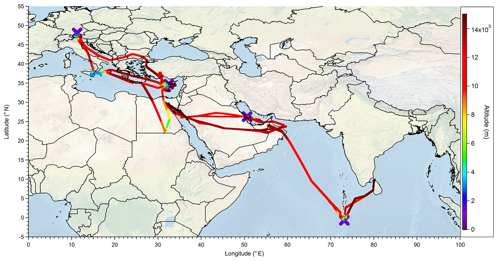
Figure 1 Flight tracks (colors indicate altitude) and airports (purple crosses) used during the OMO campaign.

3 Methods

3.1 Hydroperoxide measurements

The hydroperoxide data (${\mathrm{H}}_{\mathrm{2}}{{\mathrm{O}}_{\mathrm{2}}}^{\mathrm{obs}}$ and total organic hydroperoxides, ROOH^obs) during OMO were obtained using a modified commercial instrument (AEROLASER, model AL2021, Garmisch-Partenkirchen, Germany) called HYPHOP (hydrogen peroxide and higher organic peroxide monitor). The HYPHOP instrument was installed in a 19^′′ rack together with the infrared laser absorption instrument TRISTAR (tracer in situ TDLAS for atmospheric research) mounted in the back of HALO. Air was sampled from the top of the aircraft fuselage through a forward-facing trace gas inlet (TGI) designed as a bypass, consisting of a $\mathrm{1}/{\mathrm{2}}^{\prime \prime }$ PFA (perfluoroalkoxy alkane) tube inside the aircraft with an exit through a second TGI. From this bypass, air was sampled at a flow rate of 2 slpm (standard liters per minute) through a $\mathrm{1}/{\mathrm{4}}^{\prime \prime }$ PFA tube and directed to HYPHOP. To obtain constant pressure at the HYPHOP inlet, a constant pressure inlet (CPI) consisting of a dual-stage membrane pump (Vacuubrand MD1C VARIO SP, Wertheim, Germany) was used (Klippel et al., 2011).

HYPHOP relies on a dual-enzyme detection method after transfer of gaseous hydroperoxides into a buffered solution (potassium hydrogen phthalate and NaOH, pH 6) in a glass stripping coil (Lazrus et al., 1985, 1986). This stripper also contains EDTA (ethylenediaminetetraacetic acid) to prevent the reaction of transition metal ions with the hydroperoxides. Additionally, formaldehyde (HCHO) is added to prevent the oxidation of dissolved SO₂ (in alkaline solutions ${\mathrm{HSO}}_{\mathrm{3}}^{-}$) by the hydroperoxides. Instead, HCHO and ${\mathrm{HSO}}_{\mathrm{3}}^{-}$ form hydroxymethyl sulfonate (${\mathrm{HOCH}}_{\mathrm{2}}{\mathrm{SO}}_{\mathrm{3}}^{-}$). After the stripping coil the hydroperoxide-containing solution is divided into two channels. Catalase is added to one channel in order to selectively destroy H₂O₂. This first channel thus measures only ROOH, while the second channel (without catalase) measures the sum of ROOH and H₂O₂. Since hydroperoxides cannot be detected by fluorescence directly, a second enzyme (horseradish peroxidase) and p-hydroxyphenylacetic acid (POPHA) are added to both channels. In a quantitative and selective reaction, the enzyme catalyzes the oxidation of POPHA by hydroperoxides, forming the fluorescent dye 6,6^′-dihydroxy-3,3^′-biphenyldiacetid acid. After excitation at 326 nm with a Cd lamp, the fluorescence at 400–420 nm is detected. To enlarge the fluorescence intensity, sodium hydroxide is added.

In order to perform zero measurements, the sampled air is directed through a cylinder filled with Hopcalite (MnO₂ and CuO) to eliminate H₂O₂, ROOH, and ozone. Since the efficiency of Hopcalite decreases with increased humidity, the air is dried beforehand with the help of orange gel (SiO₂ beads plus indicator).

To convert the detected signal into a concentration, a four-point calibration was performed before and after every flight. In the first two steps a liquid standard of H₂O₂ (1 µmol L⁻¹; freshly diluted from stock solution) followed by zero air is measured in both channels without catalase. Afterwards this is repeated with catalase in the ROOH channel for the last two steps. The sensitivity for both channels and the catalase efficiency are determined via this procedure. The concentration of the liquid standard is based on titration of the stock solution (10 mmol L⁻¹) with potassium permanganate.

To determine the stripping efficiency for H₂O₂, a gas-phase standard based on a permeation source (Teflon tube filled with 30 % H₂O₂ in a temperature-controlled glass flask) is used at a constant flow rate of approximately 40 sccm, diluted with synthetic air and measured with the instrument. The permeation rate of the source is quantified by collecting the output of the source into cooled water. The addition of hydrochloric titanium tetrachloride yields the formation of the yellow η²-peroxo complex $\left[\mathrm{Ti}\right({\mathit{\eta }}^{\mathrm{2}}-{\mathrm{O}}_{\mathrm{2}}){\mathrm{Cl}}_{\mathrm{4}}{]}^{\mathrm{2}-}$ (Pilz and Johann, 1974), whose concentration is determined via a UV photometer. The stripping efficiency of MHP was assumed to be 60% and that of H₂O₂ to be 100 % (AEROLASER, 2006; Lee et al., 2000).

The inlet efficiency was determined with the help of the permeation source, which was measured with and without the CPI. In laboratory studies the inlet efficiency was determined to be 87 % ± 3 %, decreasing during the campaign to 62.7 % ± 0.8 %, which is mainly due to the higher humidity.

The limit of detection (LOD) and precisions for H₂O₂ and MHP (assuming total ROOH^obs to be only MHP), respectively, have been calculated for each flight from the reproducibility (1σ standard deviation) of in-flight zero (650 values) and liquid calibration (100 values) measurements, taking into account the sensitivity, stripping, and catalase efficiency. LOD values are in the range of 8–53 ppt_v for ${\mathrm{H}}_{\mathrm{2}}{{\mathrm{O}}_{\mathrm{2}}}^{\mathrm{obs}}$ (median 23 ppt_v) and 9–52 ppt_v for ROOH^obs (median 23 ppt_v), respectively, assuming that ROOH^obs is composed of MHP only. Please note that due to the fact that the exact composition of ROOH^obs is unknown, and the solubility of different ROOH species can be quite variable, a detection limit for ROOH^obs cannot be given. Instead, we calculate an upper limit of the detection limit, assuming that all ROOH^obs consists of MHP, the species with the smallest solubility. Precision values were determined from the reproducibility of standard measurements and are in the range of 0.2 % at 5.2 ppb_v and 1.3 % at 5.9 ppb_v for H₂O₂ and 0.3 % at 5.0 ppb_v and 2.1 % at 6.0 ppb_v for MHP. The time resolution (signal increase from 10 % to 90 %) of the instrument is 120 s. An ozone interference of 53 ppt_v H₂O₂ per 100 ppb_v O₃, which was determined by H₂O₂ measurements in the stratosphere during the OMO-EU test campaign, was taken into account and corrected.

The total uncertainty calculated from statistical errors and uncertainties of liquid standard, inlet and stripping efficiency, and ozone interference is 25 % for H₂O₂ and 40 % for MHP.

3.2 Other in situ measurements

For this study CO, CH₄, OH, HO₂, O₃, acetone, NO, NO_y, $J_{{\mathrm{H}}_{\mathrm{2}}{\mathrm{O}}_{\mathrm{2}}}$, and J_MHP data measured by other instruments have been used for data interpretation, steady-state calculations, and interference corrections (see Sect. 3.1). A complete list of all measured compounds can be found in Lelieveld et al. (2018). CO and CH₄ have been measured by the IR quantum cascade laser absorption spectrometer TRISTAR (Schiller et al., 2008; Tadic et al., 2017). The measurements comprised an ambient-air mode and in-flight calibrations. The latter were realized with secondary standards from pressurized bottles (6 L bottle, Auer GmbH, Germany), which were calibrated against certified reference gases (Tomsche et al., 2019). With the help of the in-flight calibrations, the in situ data are drift-corrected by interpolation between two calibrations (Tadic et al., 2017). The observed CO and CH₄ mixing ratios have a total uncertainty of 5.1 % and 0.275 %, respectively. The relatively high CO uncertainty reflects problems with the stability of the CO quantum cascade laser during the second half of OMO.

Laser-induced fluorescence was the method utilized for HO_x measurements (instrument name: HORUS; Faloona et al., 2004; Martinez et al., 2010). The accuracies of the measurements are 17.1 % for OH and 17.6 % for HO₂. The limit of detection of the instrument does vary depending on altitude as this system has a sensitivity that depends on pressure. As altitude increases the LOD decreases from 0.1 ppt_v to 0.02 ppt_v for OH and 0.361 to 0.175 ppt_v for HO₂.

FAIRO (fast airborne ozone instrument) is a lightweight (14.5 kg) and accurate two-sensor device for measuring O₃. It combines two techniques, i.e., (a) a UV photometer that measures the light absorption by O₃ at a wavelength of λ = 250–260 nm emitted by a UV-LED and (b) a chemiluminescence detector that monitors the chemiluminescence generated by O₃ on the surface of an organic dye adsorbed on dry silica gel. These techniques are simultaneously applied in order to combine the high measurement accuracy of the UV photometry with the high measurement frequency of the chemiluminescence detection. The UV photometer has a 1σ precision of 0.08 ppb_v at a measurement frequency of 0.25 Hz (and a pressure of 1 bar) and an accuracy of 1.5 % (determined by the uncertainty of the O₃ cross section). The chemiluminescence detector has a precision of 0.05 ppb_v at a measurement frequency of 12.5 Hz (Zahn et al., 2012). In postprocessing the chemiluminescence detector data are calibrated using the UV photometer data.

Nitrogen oxide (NO) and total reactive nitrogen (NO_y) were measured using the AENEAS atmospheric nitrogen oxide measuring system. The measurements were performed by a dual-channel NO chemiluminescence detector (CLD-SR 790, Eco Physics, Switzerland) in combination with a converter technique for the detection of total reactive nitrogen as NO. NO_y comprises, among others, NO, NO₂, HNO₃, NO₃, N₂O₅, HNO₂, HO₂NO₂, PAN, and organic nitrates. The individual NO_y species were detected after conversion to NO using a gold tube maintained at about 300 ^∘C, with H₂ as a reducing agent (Ziereis et al., 2000). Ambient air was sampled using a standard HALO trace gas inlet equipped with a heated (∼40 ^∘C) PFA inlet line. The time resolution of the measurements was about 1 s. The overall uncertainty of the NO and NO_y measurements depends on its ambient concentrations and is about 8 % (6.5 %) for volume mixing ratios of 0.5 nmol mol⁻¹ (1 nmol mol⁻¹), respectively (Stratmann et al., 2016).

VOCs (e.g., acetone) were measured with a homebuilt lightweight (∼55 kg without rack) proton-transfer-reaction mass spectrometer, which uses a commercial quadrupole mass analyzer (Pfeiffer, QMA 410, Germany). A modular V25 microcomputer system (MPI-C, Mainz, Germany) is applied for instrument control and data acquisition. A custom-built inlet system comprises a platinum–quartz wool scrubber (Shimadzu, High Sensitivity Catalyst) held at 300 ^∘C and components for flow and pressure control. The instrument was calibrated between flights with a dynamically diluted gas standard containing approximately 500 ppb_v of VOCs (Apel-Riemer Environmental Inc., USA). The accuracy for acetone is typically ±10 %, and the detection limit is ∼60 ppt_v.

Photolysis frequencies were calculated from spectral actinic flux density spectra (280–650 nm) obtained from charge-coupled device (CCD) spectroradiometer measurements on the top and bottom fuselage of the aircraft, covering the upper and the lower hemisphere, respectively (Bohn and Lohse, 2017). Recent recommendations of absorption cross sections and quantum yields were used in the calculations as well as their temperature and pressure dependencies (if available) by taking into account measured static air temperatures and pressures. Radiometric uncertainties range around 5 %–6 % under typical flight conditions. Additional uncertainties related to the molecular parameters are process-specific. For H₂O₂ in particular, recommended absorption cross sections and their temperature dependencies were applied, and unity quantum yields were assumed (Burkholder et al., 2015). However, the recommended H₂O₂ absorption cross sections are confined to a wavelength range below 350 nm, which is insufficient to capture atmospheric photolysis completely. Because measured cross sections decay exponentially over 2 orders of magnitude in the range of 280–350 nm, this dependence was further extrapolated up to 370 nm, where values drop well below 10⁻²² cm². Dependent on conditions, this extrapolation increases atmospheric H₂O₂ photolysis frequencies by 10 %–20 %. For MHP the temperature dependence of the absorption cross sections is unknown. Therefore the recommended room temperature data were used under all conditions as well as unity quantum yields (Burkholder et al., 2015). Combined total uncertainties of 15 % and 25 % are estimated for H₂O₂ and MHP photolysis frequencies, respectively.

Latitude, longitude, and altitude data as well as temperature and pressure were collected with the BAHAMAS (basic HALO measurement and sensor system) instrument. More detailed information about the installation of scientific instruments and mission flights can be found at http://www.halo.dlr.de/science/missions/omo/omo.html (last access: 27 February 2019).

3.3 Photostationary-state calculations

Since only the sum of organic hydroperoxides was measured, we estimated the contribution of MHP using a photostationary-state (PSS) approximation relying on in situ measurements of HO₂, OH, CO, CH₄, NO, J_MHP, and $J_{{\mathrm{H}}_{\mathrm{2}}{\mathrm{O}}_{\mathrm{2}}}$ (see Sect. 3.2) and rate coefficient data from Atkinson et al. (2004, 2006).

In the free troposphere the production rate P of H₂O₂ and MHP is due to the self-reaction of HO₂ and reaction of CH₃O₂ with HO₂, respectively, and can be calculated from Eqs. (1) and (2).

$$\begin{array}{}\text{(1)}& {\displaystyle }P\left({\mathrm{H}}_{\mathrm{2}}{\mathrm{O}}_{\mathrm{2}}\right)=k_{{\mathrm{HO}}_{\mathrm{2}}+{\mathrm{HO}}_{\mathrm{2}}}\cdot {\left[{\mathrm{HO}}_{\mathrm{2}}\right]}^{\mathrm{2}}\text{(2)}& {\displaystyle }P\left(\mathrm{MHP}\right)=k_{{\mathrm{CH}}_{\mathrm{3}}{\mathrm{O}}_{\mathrm{2}}+{\mathrm{HO}}_{\mathrm{2}}}\cdot \left[{\mathrm{CH}}_{\mathrm{3}}{\mathrm{O}}_{\mathrm{2}}\right]\cdot \left[{\mathrm{HO}}_{\mathrm{2}}\right]\end{array}$$

Photochemical loss rates L of H₂O₂ and MHP are due to photolysis and reaction with OH according to Eqs. (3) and (4).

$$\begin{array}{}\text{(3)}& {\displaystyle }L\left({\mathrm{H}}_{\mathrm{2}}{\mathrm{O}}_{\mathrm{2}}\right)=\left(k_{{\mathrm{H}}_{\mathrm{2}}{\mathrm{O}}_{\mathrm{2}}+\mathrm{OH}}\cdot \left[\mathrm{OH}\right]+J_{{\mathrm{H}}_{\mathrm{2}}{\mathrm{O}}_{\mathrm{2}}}\right)\cdot \left[{\mathrm{H}}_{\mathrm{2}}{\mathrm{O}}_{\mathrm{2}}\right]\text{(4)}& {\displaystyle }L\left(\mathrm{MHP}\right)=\left(k_{\mathrm{MHP}+\mathrm{OH}}\cdot \left[\mathrm{OH}\right]+J_{\mathrm{MHP}}\right)\cdot \left[\mathrm{MHP}\right]\end{array}$$

For steady-state conditions the production and loss reactions are at equilibrium, and the MHP^PSS-to-${\mathrm{H}}_{\mathrm{2}}{{\mathrm{O}}_{\mathrm{2}}}^{\mathrm{obs}}$ ratio can be calculated from Eq. (5).

$$\begin{array}{}\text{(5)}& \begin{array}{rl}{\displaystyle \frac{{\left[\mathrm{MHP}\right]}^{\mathrm{PSS}}}{{\left[{\mathrm{H}}_{\mathrm{2}}{\mathrm{O}}_{\mathrm{2}}\right]}^{\mathrm{obs}}}}& ={\displaystyle \frac{k_{{\mathrm{CH}}_{\mathrm{3}}{\mathrm{O}}_{\mathrm{2}}+{\mathrm{HO}}_{\mathrm{2}}}\cdot \left[{\mathrm{CH}}_{\mathrm{3}}{\mathrm{O}}_{\mathrm{2}}\right]\cdot \left[{\mathrm{HO}}_{\mathrm{2}}\right]}{k_{{\mathrm{HO}}_{\mathrm{2}}+{\mathrm{HO}}_{\mathrm{2}}}\cdot {\left[{\mathrm{HO}}_{\mathrm{2}}\right]}^{\mathrm{2}}}}\\ & \cdot {\displaystyle \frac{k_{{\mathrm{H}}_{\mathrm{2}}{\mathrm{O}}_{\mathrm{2}}+\mathrm{OH}}\cdot \left[\mathrm{OH}\right]+J_{{\mathrm{H}}_{\mathrm{2}}{\mathrm{O}}_{\mathrm{2}}}}{k_{\mathrm{MHP}+\mathrm{OH}}\cdot \left[\mathrm{OH}\right]+J_{\mathrm{MHP}}}}\end{array}\end{array}$$

Because individual peroxy radicals were not measured, the CH₃O₂-to-HO₂ ratio must be estimated from their production and loss terms. This ratio can be deduced as written in Eq. (6).

$$\begin{array}{}\text{(6)}& {\displaystyle \frac{\left[{\mathrm{CH}}_{\mathrm{3}}{\mathrm{O}}_{\mathrm{2}}\right]}{\left[{\mathrm{HO}}_{\mathrm{2}}\right]}}={\displaystyle \frac{L\left({\mathrm{HO}}_{\mathrm{2}}\right)\cdot P\left({\mathrm{CH}}_{\mathrm{3}}{\mathrm{O}}_{\mathrm{2}}\right)}{P\left({\mathrm{HO}}_{\mathrm{2}}\right)\cdot L\left({\mathrm{CH}}_{\mathrm{3}}{\mathrm{O}}_{\mathrm{2}}\right)}}\end{array}$$

Dominant loss processes for HO₂ and CH₃O₂ are reactions with NO and the production of H₂O₂ and MHP, respectively, neglecting the production of peroxy nitrates due to low NO₂ concentrations in the UT (Eqs. 7 and 8).

$$\begin{array}{}\text{(7)}& {\displaystyle }\begin{array}{rl}L\left({\mathrm{HO}}_{\mathrm{2}}\right)& =k_{{\mathrm{CH}}_{\mathrm{3}}{\mathrm{O}}_{\mathrm{2}}+{\mathrm{HO}}_{\mathrm{2}}}\cdot \left[{\mathrm{CH}}_{\mathrm{3}}{\mathrm{O}}_{\mathrm{2}}\right]\cdot \left[{\mathrm{HO}}_{\mathrm{2}}\right]+k_{{\mathrm{HO}}_{\mathrm{2}}+\mathrm{NO}}\\ & \cdot \left[{\mathrm{HO}}_{\mathrm{2}}\right]\cdot \left[\mathrm{NO}\right]+k_{{\mathrm{HO}}_{\mathrm{2}}+{\mathrm{HO}}_{\mathrm{2}}}\cdot {\left[{\mathrm{HO}}_{\mathrm{2}}\right]}^{\mathrm{2}}\end{array}\text{(8)}& {\displaystyle }\begin{array}{rl}L\left({\mathrm{CH}}_{\mathrm{3}}{\mathrm{O}}_{\mathrm{2}}\right)& =k_{{\mathrm{CH}}_{\mathrm{3}}{\mathrm{O}}_{\mathrm{2}}+{\mathrm{HO}}_{\mathrm{2}}}\cdot \left[{\mathrm{CH}}_{\mathrm{3}}{\mathrm{O}}_{\mathrm{2}}\right]\cdot \left[{\mathrm{HO}}_{\mathrm{2}}\right]\\ & +k_{{\mathrm{CH}}_{\mathrm{3}}{\mathrm{O}}_{\mathrm{2}}+\mathrm{NO}}\cdot \left[{\mathrm{CH}}_{\mathrm{3}}{\mathrm{O}}_{\mathrm{2}}\right]\cdot \left[\mathrm{NO}\right]\end{array}\end{array}$$

The first terms on the right side of both equations are identical. The second terms are dominated by the rate coefficients of the reactions with NO and the NO concentration. For the calculations of the rate coefficients, the mean temperature of 259.18 K, the mean altitude of 10 992.8 m, and the mean pressure of 22 932.9 Pa were used. The resulting values are shown in Eqs. (9)–(11). As the relative humidity is very low in the upper troposphere, the water dependence in Eq. (11) was neglected.

$$\begin{array}{}\text{(9)}& {\displaystyle }\begin{array}{rl}{k}_{{\mathrm{HO}}_{\mathrm{2}}+\mathrm{NO}}& =\mathrm{3.45}\times {\mathrm{10}}^{-\mathrm{12}}\cdot {\exp }^{\frac{\mathrm{270}}{T}}\\ & =\mathrm{9.78}\times {\mathrm{10}}^{-\mathrm{12}}{\mathrm{cm}}^{\mathrm{3}}(\mathrm{molec}.\mathrm{s}{)}^{-\mathrm{1}}\end{array}\text{(10)}& {\displaystyle }\begin{array}{rl}{k}_{{\mathrm{CH}}_{\mathrm{3}}{\mathrm{O}}_{\mathrm{2}}+\mathrm{NO}}& =\mathrm{2.3}\times {\mathrm{10}}^{-\mathrm{12}}\cdot {\exp }^{\frac{\mathrm{360}}{T}}\\ & =\mathrm{9.22}\times {\mathrm{10}}^{-\mathrm{12}}{\mathrm{cm}}^{\mathrm{3}}(\mathrm{molec}.\mathrm{s}{)}^{-\mathrm{1}}\end{array}\text{(11)}& {\displaystyle }\begin{array}{rl}{k}_{{\mathrm{HO}}_{\mathrm{2}}+{\mathrm{HO}}_{\mathrm{2}}}& =\mathrm{2.2}\times {\mathrm{10}}^{-\mathrm{13}}\cdot {\exp }^{\frac{\mathrm{600}}{T}}\\ & +\mathrm{1.9}\times {\mathrm{10}}^{-\mathrm{33}}\cdot \left[{\mathrm{N}}_{\mathrm{2}}\right]\cdot {\exp }^{\frac{\mathrm{980}}{T}}\\ & =\mathrm{2.64}\times {\mathrm{10}}^{-\mathrm{12}}{\mathrm{cm}}^{\mathrm{3}}(\mathrm{molec}.\mathrm{s}{)}^{-\mathrm{1}}\end{array}\end{array}$$

This indicates that the reaction of HO₂ with NO is more than a factor of 3 faster than the self-reaction. The measured NO concentration is an order of magnitude larger than measured HO₂ so that reaction with NO is the dominant process for both HO₂ and CH₃O₂, resulting in similar loss rates for both radicals in the UT. Thus, the ratio of CH₃O₂ to HO₂ is dominated by their production rates (Eq. 12).

$$\begin{array}{}\text{(12)}& {\displaystyle \frac{\left[{\mathrm{CH}}_{\mathrm{3}}{\mathrm{O}}_{\mathrm{2}}\right]}{\left[{\mathrm{HO}}_{\mathrm{2}}\right]}}={\displaystyle \frac{P\left({\mathrm{CH}}_{\mathrm{3}}{\mathrm{O}}_{\mathrm{2}}\right)}{P\left({\mathrm{HO}}_{\mathrm{2}}\right)}}={\displaystyle \frac{k_{{\mathrm{CH}}_{\mathrm{4}}+\mathrm{OH}}\cdot \left[{\mathrm{CH}}_{\mathrm{4}}\right]\cdot \left[\mathrm{OH}\right]}{k_{\mathrm{CO}+\mathrm{OH}}\cdot \left[\mathrm{CO}\right]\cdot \left[\mathrm{OH}\right]}}\end{array}$$

The combination of Eqs. (5) and (12) results in Eq. (13), which was used to calculate the MHP^PSS concentrations based on the observed mixing ratios during OMO.

$$\begin{array}{}\text{(13)}& \begin{array}{rl}{\left[\mathrm{MHP}\right]}^{\mathrm{PSS}}& ={\displaystyle \frac{k_{{\mathrm{CH}}_{\mathrm{3}}{\mathrm{O}}_{\mathrm{2}}+{\mathrm{HO}}_{\mathrm{2}}}}{k_{{\mathrm{HO}}_{\mathrm{2}}+{\mathrm{HO}}_{\mathrm{2}}}}}\\ & \cdot {\displaystyle \frac{k_{{\mathrm{H}}_{\mathrm{2}}{\mathrm{O}}_{\mathrm{2}}+\mathrm{OH}}\cdot {\left[\mathrm{OH}\right]}^{\mathrm{obs}}+J_{{\mathrm{H}}_{\mathrm{2}}{\mathrm{O}}_{\mathrm{2}}}^{\mathrm{obs}}}{k_{\mathrm{MHP}+\mathrm{OH}}\cdot }}\cdot {\left[\mathrm{OH}\right]}^{\mathrm{obs}}\\ & +J_{\mathrm{MHP}}^{\mathrm{obs}}\cdot {\displaystyle \frac{k_{{\mathrm{CH}}_{\mathrm{4}}+\mathrm{OH}}\cdot {\left[{\mathrm{CH}}_{\mathrm{4}}\right]}^{\mathrm{obs}}}{k_{\mathrm{CO}+\mathrm{OH}}\cdot {\left[\mathrm{CO}\right]}^{\mathrm{obs}}}}\cdot {\left[{\mathrm{H}}_{\mathrm{2}}{\mathrm{O}}_{\mathrm{2}}\right]}^{\mathrm{obs}}\end{array}\end{array}$$

Please note that other sources of HO₂ and CH₃O₂, in particular the photolysis of formaldehyde (HCHO) and acetaldehyde, respectively have been neglected. This is justified by the generally low mixing ratios of these species at high altitudes. Measurements of HCHO with the TRISTAR instrument yielded values below the detection limit of 30 ppt_v (parts per trillion by volume), and although acetaldehyde was not measured, we assume that its mixing ratio is within a factor of 2 of those for HCHO.

The total uncertainty of MHP^PSS from the calculation according to Eq. (13) can be deduced from error propagation, taking into account uncertainties in OH^obs (17.1 %), $J_{{\mathrm{H}}_{\mathrm{2}}{\mathrm{O}}_{\mathrm{2}}}^{\mathrm{obs}}$ (15 %), $J_{\mathrm{MHP}}^{\mathrm{obs}}$ (25 %), ${\mathrm{CH}}_{\mathrm{4}}^{\mathrm{obs}}$ (0.275 %), CO^obs (5.1 %), ${\mathrm{H}}_{\mathrm{2}}{{\mathrm{O}}_{\mathrm{2}}}^{\mathrm{obs}}$ (25 %), and rate constants, to be of the order of 45 % (1σ).

To estimate the contribution of MHP to the total organic hydroperoxides, the calculated concentration of MHP^PSS was subtracted from the measured sum of all organic hydroperoxides ROOH^obs. This leads to a concentration of unidentified organic hydroperoxides (UHP^PSS; Eq. 14). Please note that MHP^PSS only accounts for local CH₄ oxidation production and not for transport phenomena.

$$\begin{array}{}\text{(14)}& {\left[\mathrm{UHP}\right]}^{\mathrm{PSS}}={\left[\mathrm{ROOH}\right]}^{\mathrm{obs}}-[\mathrm{MHP}{]}^{\mathrm{PSS}}\end{array}$$

3.4 H₂O₂ calculation

In order to classify the measured ${\mathrm{H}}_{\mathrm{2}}{{\mathrm{O}}_{\mathrm{2}}}^{\mathrm{obs}}$, ${{\mathrm{HO}}_{\mathrm{2}}}^{\mathrm{obs}}$, and OH^obs data, we calculated ${\mathrm{H}}_{\mathrm{2}}{{\mathrm{O}}_{\mathrm{2}}}^{\mathrm{PSS}}$ from measured HO_x and $J_{{\mathrm{H}}_{\mathrm{2}}{\mathrm{O}}_{\mathrm{2}}}^{\mathrm{obs}}$. For the calculation, Eq. (15) was used, which is based on Eqs. (1) and (3).

$$\begin{array}{}\text{(15)}& {\left[{\mathrm{H}}_{\mathrm{2}}{\mathrm{O}}_{\mathrm{2}}\right]}^{\mathrm{PSS}}={\displaystyle \frac{{\left[{\mathrm{HO}}_{\mathrm{2}}\right]}^{\mathrm{obs}\mathrm{2}}\cdot k_{{\mathrm{HO}}_{\mathrm{2}}+{\mathrm{HO}}_{\mathrm{2}}}}{{\left[\mathrm{OH}\right]}^{\mathrm{obs}}\cdot k_{{\mathrm{H}}_{\mathrm{2}}{\mathrm{O}}_{\mathrm{2}}+\mathrm{OH}}+J_{{\mathrm{H}}_{\mathrm{2}}{\mathrm{O}}_{\mathrm{2}}}^{\mathrm{obs}}}}\end{array}$$

A total uncertainty of 45 % (1σ) due to uncertainties in OH^obs (17.1 %), ${{\mathrm{HO}}_{\mathrm{2}}}^{\mathrm{obs}}$ (17.6 %), $J_{{\mathrm{H}}_{\mathrm{2}}{\mathrm{O}}_{\mathrm{2}}}^{\mathrm{obs}}$ (15 %), and reaction rate constants was calculated.

3.5 Other research tools

The EMAC (ECHAM–MESSy atmospheric chemistry) model comprises the fifth generation of the European Center Hamburg (ECHAM5; Roeckner et al., 2006; version 5.3.01) general circulation model and the Modular Earth Submodel System (MESSy; Jöckel et al., 2016; version 2.52, http://www.messy-interface.org/, last access: 25 August 2019). For this study EMAC simulations (T42L90, 2.8^∘ × 2.8^∘ horizontal resolution, 90 vertical levels to 0.01 hPa, time resolution 12 min) were sampled along the OMO flights tracks. Detailed specifications and results have been published previously (Lelieveld et al., 2018; Tomsche et al., 2019).

Back trajectories of 10 d were calculated along the flight path using FLEXPART to identify the air mass origin (Tomsche et al., 2019). Convective transport can be simulated in FLEXPART with the convection parameterization by Emanuel and Zivkovic-Rothman (1999). To represent moist convection realistically in models, the parametrization includes cloud microphysical processes, the physics of entrainment and mixing, and large-scale control of ensemble convective activity. It builds on temperature and humidity fields to provide mass flux information (Stohl et al., 2005). The back trajectories in the present paper are calculated with the convective parametrization. Further, the Lagrangian particle dispersion model FLEXPART produces so-called centroid trajectories based on the analysis of a cluster of trajectories. These trajectories are comparable to traditional trajectories but include convection via the centroid of all particles per time step. As indicated by Tomsche et al. (2019), prominent source regions of AMA air masses are identified to be the Indo-Gangetic Plain, northeastern India, Bangladesh, and the Bay of Bengal. Additionally, Tomsche et al. used observations of methane to differentiate between air masses influenced by the AMA and background air. A comparison of vertical profiles indicated that the air inside the AMA showed significantly higher CH₄ concentrations than outside. Thus a threshold of CH₄≥1879.8 ppb_v was used to distinguish between air masses influenced by the AMA (CH₄≥1879.8 ppb_v), the SH background (CH₄<1820 ppb_v), and the NH background (1820 ppb${}_{\mathrm{v}}\le {\mathrm{CH}}_{\mathrm{4}}<\mathrm{1879.8}$ ppb_v; Tomsche et al., 2019).

4 Results and discussion

4.1 Data processing

Data were collected from a merged data set given as 60 s means (calculated from the original data set obtained at higher resolutions) in order to get the same time resolution for all compounds. The given time is the middle of the block mean.

For the histograms the concentrations of all species shown were binned into samples with a width of 10 ppt_v, starting with the plots with the lowest bin. To compare the simulations from EMAC with measured and PSS-calculated data, the corresponding values (out of the 60 s means) were used at the given times from EMAC.

4.2 Case study: Flight 17 from Gan to Bahrain (10 August 2015)

In a case study analyzing Flight 17 from 10 August 2015, the method used to determine the origin of the measured air masses and a quantification and comparison of measured and simulated mixing ratios of ${\mathrm{H}}_{\mathrm{2}}{{\mathrm{O}}_{\mathrm{2}}}^{\mathrm{obs}}$, MHP^PSS, and UHP^PSS is presented. During this flight we encountered the SH and NH as well as the AMA in the UT. The flight track is shown in Fig. 2 (dotted line). Takeoff was in Gan (Maldives) and landing in Bahrain, on the Arabian Peninsula. Besides takeoff and landing, the entire flight took place in the UT (<230 hPa). The calculated back trajectories show the origin of the air masses. At the beginning of the flight the measured air masses had their origin over the Indian Ocean and Indonesia. During the remaining flight the measured air stemmed from India. Tomsche et al. (2019) showed that the measured air in the AMA was affected by deep convection over India, resulting in methane mixing ratios above the threshold. Figure 3 shows the time series for ${\mathrm{H}}_{\mathrm{2}}{{\mathrm{O}}_{\mathrm{2}}}^{\mathrm{obs}}$ during the flight at the time steps given from the frequency of EMAC output (orange circles). The colored bar on top shows the origin of air masses, i.e., red for AMA, green for NH, and blue for SH. The ${\mathrm{H}}_{\mathrm{2}}{{\mathrm{O}}_{\mathrm{2}}}^{\mathrm{obs}}$ mixing ratios vary between 128 and 366 ppt_v. The modeled ${\mathrm{H}}_{\mathrm{2}}{{\mathrm{O}}_{\mathrm{2}}}^{\mathrm{EMAC}}$ data are in the range of 110–799 ppt_v (gray triangles). For the beginning of the flight, model simulations agree rather well with the measurement data. At around 06:00 UTC the model-calculated mixing ratios increase to more than 500 ppt_v, while the measured data decrease to 200 ppt_v and lower. In this period a maximum difference between model and in situ data of 386 ppt_v was found. After 1 h the EMAC model data decrease to 416 ppt_v, and the in situ data increase to 214 ppt_v. During the following hour until around 08:00 UTC and thus at higher altitude, both mixing ratios increase, with the modeled data showing a much stronger increase up to approximately 800 ppt_v, while the in situ data increase only to 230 ppt_v. During the last period of the flight, simulated and measured data are again in good agreement. Here the mixing ratios from EMAC are in the range of 110–157 ppt_v, while the measured data are in the range of 128–203 ppt_v. This steep drop of ${\mathrm{H}}_{\mathrm{2}}{{\mathrm{O}}_{\mathrm{2}}}^{\mathrm{EMAC}}$ might arise due to a change in the flight altitude since between 08:01 and 08:06 UTC the aircraft changed from a flight level at 11 700 m to one aloft at 13 900 m.

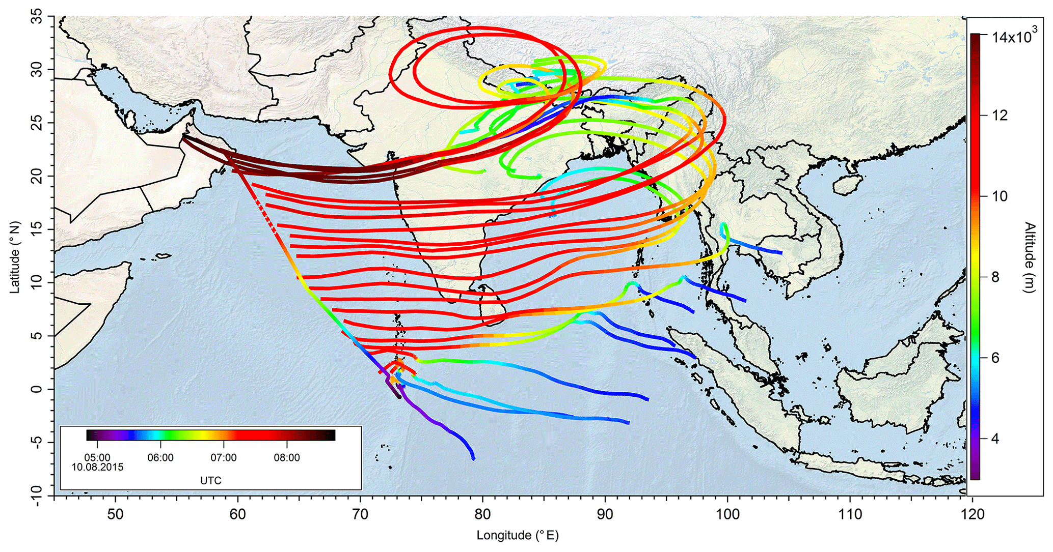
Figure 2 Track of Flight 17 (dotted black line) and calculated 10 d back trajectories (lines colored as a function of altitude) to show the origin of sampled air masses during the flight.

In addition to EMAC simulations, Fig. 3 also shows the calculated ${\mathrm{H}}_{\mathrm{2}}{{\mathrm{O}}_{\mathrm{2}}}^{\mathrm{PSS}}$ obtained from Eq. (15). Observed and PSS values for H₂O₂ mixing ratios agree very well, with a median deviation of 42 ppt_v, well within the combined uncertainties of measured data (25 %) and PSS simulations (45 %).

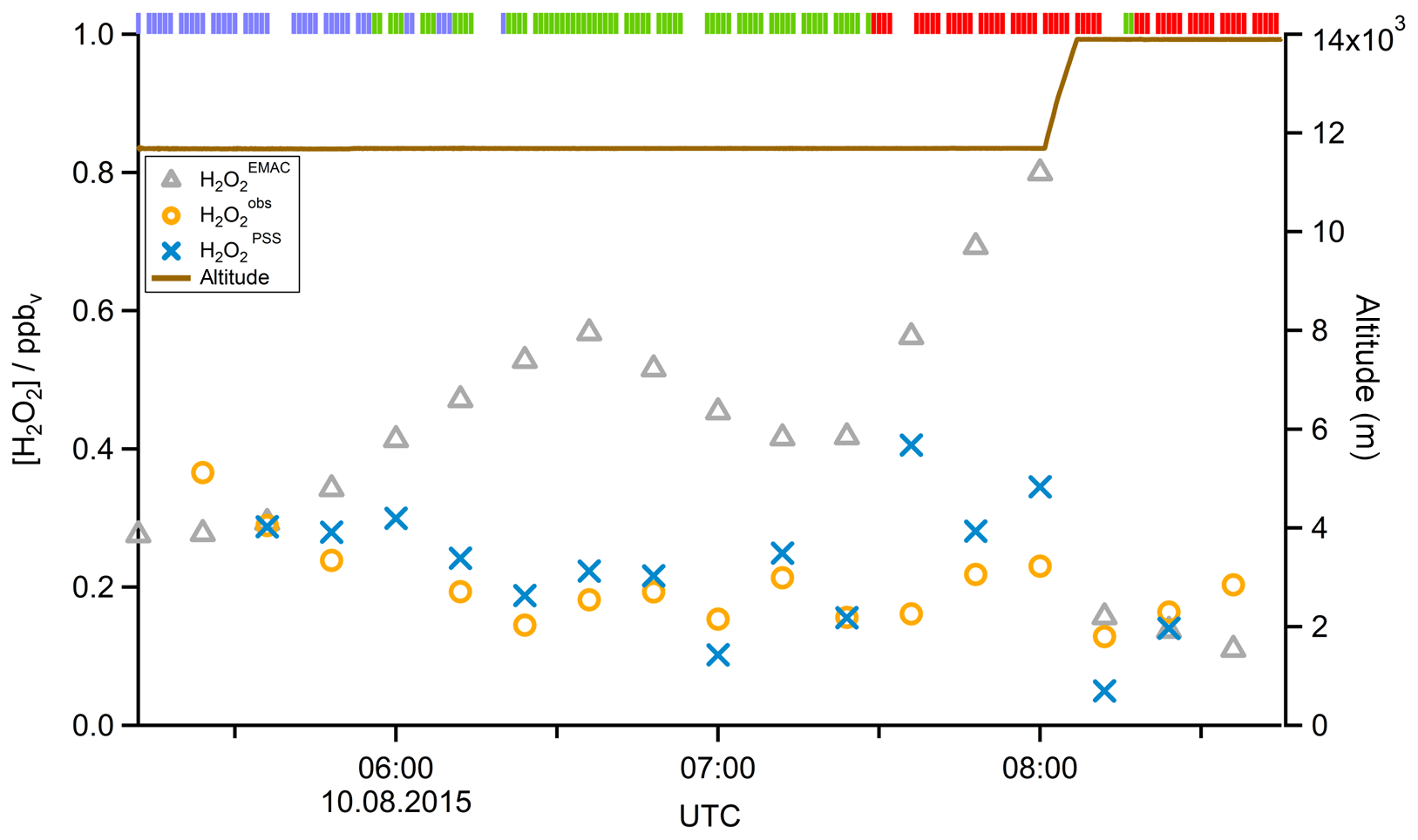
Figure 3 Time series of ${\mathrm{H}}_{\mathrm{2}}{{\mathrm{O}}_{\mathrm{2}}}^{\mathrm{obs}}$ (orange circles), ${\mathrm{H}}_{\mathrm{2}}{{\mathrm{O}}_{\mathrm{2}}}^{\mathrm{PSS}}$ (blue crosses), and ${\mathrm{H}}_{\mathrm{2}}{{\mathrm{O}}_{\mathrm{2}}}^{\mathrm{EMAC}}$ (gray triangles) mixing ratios for Flight 17. The brown line shows the altitude; the colored bar on top indicates the origin of air masses according to the methane mixing ratio classification: for SH blue, NH green, and AMA red.

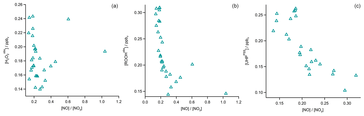
In Fig. 4 the time series of ${\mathrm{H}}_{\mathrm{2}}{{\mathrm{O}}_{\mathrm{2}}}^{\mathrm{obs}}$, MHP^PSS, and UHP^PSS mixing ratios are shown (5 min means). In the beginning of the flight, MHP^PSS is the dominant organic hydroperoxide. The mixing ratios are in the range of 140–341 ppt_v, similar to those of ${\mathrm{H}}_{\mathrm{2}}{{\mathrm{O}}_{\mathrm{2}}}^{\mathrm{obs}}$ (143–337 ppt_v). UHP^PSS mixing ratios are in the range of 24–162 ppt_v, with a mean of 89 ppt_v. Later during the flight, UHP^PSS are the dominant hydroperoxides in air masses inside the AMA originating from India. Here we found UHP^PSS mixing ratios up to 275 ppt_v. The ${\mathrm{H}}_{\mathrm{2}}{{\mathrm{O}}_{\mathrm{2}}}^{\mathrm{obs}}$ mixing ratios show a similar temporal pattern and mixing ratio levels to those of UHP^PSS over the Arabian Sea and the Arabian Peninsula, with values in the range of 140–243 ppt_v. MHP^PSS mixing ratios are much lower (62–130 ppt_v, median of 72 ppt_v) in this area. During this part of the flight, the similarity in the time series of acetone and UHP^PSS (Fig. 5) indicates either similar source regions for both species or the role of acetone as a precursor for the UHP^PSS in AMA-influenced air masses. From 06:20 UTC onwards an increase in both compounds is observed until 07:45 UTC, followed by a steep drop, with a minimum at 08:17 UTC. The UHP^PSS and acetone mixing ratios in this part of the flight are strongly correlated (Fig. 6), with a slope of 0.19±0.02 (ppb_v ppb_v⁻¹) and an offset of ($-\mathrm{0.003}\pm \mathrm{0.02}$) ppb_v. The regression coefficient R² is very high (0.82). For ${\mathrm{H}}_{\mathrm{2}}{{\mathrm{O}}_{\mathrm{2}}}^{\mathrm{obs}}$, MHP^PSS, and ROOH^obs the correlation is not that strong, with slopes of $-\mathrm{0.02}\pm \mathrm{0.02}$ (ppb_v ppb_v⁻¹), $-\mathrm{0.07}\pm \mathrm{0.01}$ (ppb_v ppb_v⁻¹), and 0.13±0.03 (ppb_v ppb_v⁻¹), respectively, and offsets of (0.21±0.02) ppb_v, (0.12±0.01) ppb_v, and (0.11±0.03) ppb_v (Fig. 6). The relation between ROOH mixing ratios and an air mass age tracer based on the ratio between [NO] and [NO_y] shows higher values of ROOH at smaller ratios, representing older or more processed air masses (Fig. 7) since the highest ROOH mixing ratios (>200 ppt_v) are found at the lowest [NO] ∕ [NO_y] ratios (all <0.19). Thus, most of the observed ROOH were measured in aged air masses transported within the anticyclone. The correlation with UHP^PSS shows that this effect is mainly due to UHP^PSS. For ${\mathrm{H}}_{\mathrm{2}}{{\mathrm{O}}_{\mathrm{2}}}^{\mathrm{obs}}$ there are also some higher mixing ratios for high [NO]-to-[NO_y] mixing ratios and thus fresher air (Fig. 7).

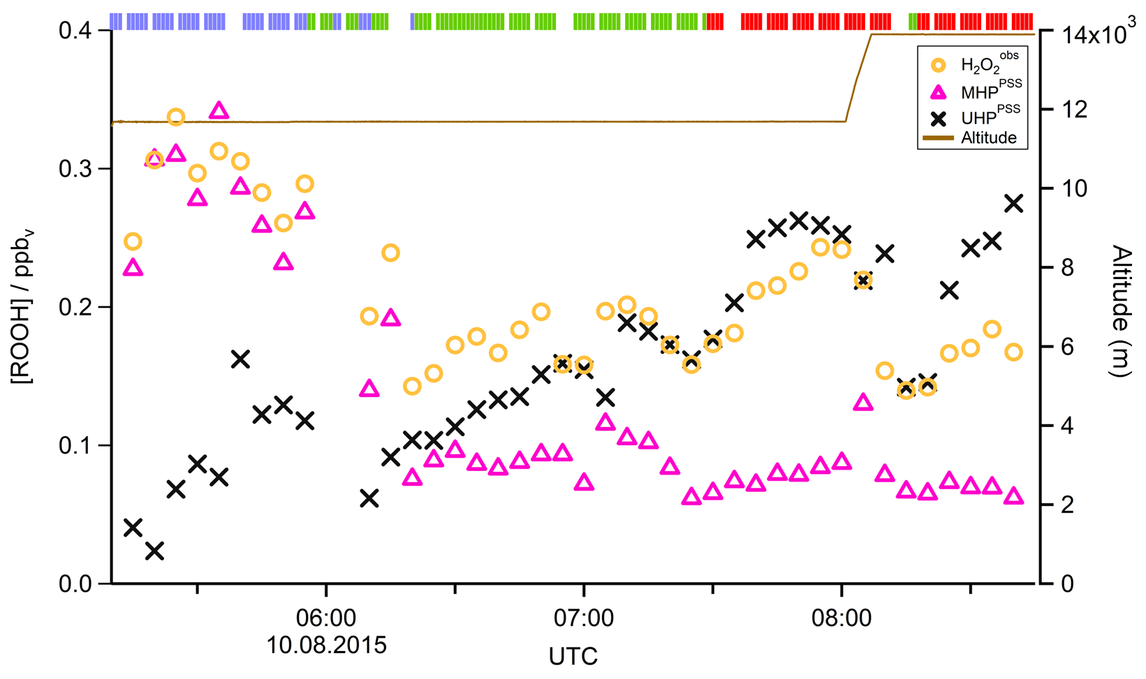
Figure 4 Time series of hydroperoxide mixing ratios during Flight 17. The mixing ratios of ${\mathrm{H}}_{\mathrm{2}}{{\mathrm{O}}_{\mathrm{2}}}^{\mathrm{obs}}$ (orange circles), MHP^PSS (pink triangles), and UHP^PSS (black crosses) are shown. The brown line shows the altitude; the colored bar on top indicates the origin of air masses according to the methane mixing ratio classification: for SH blue, NH green, and AMA red.

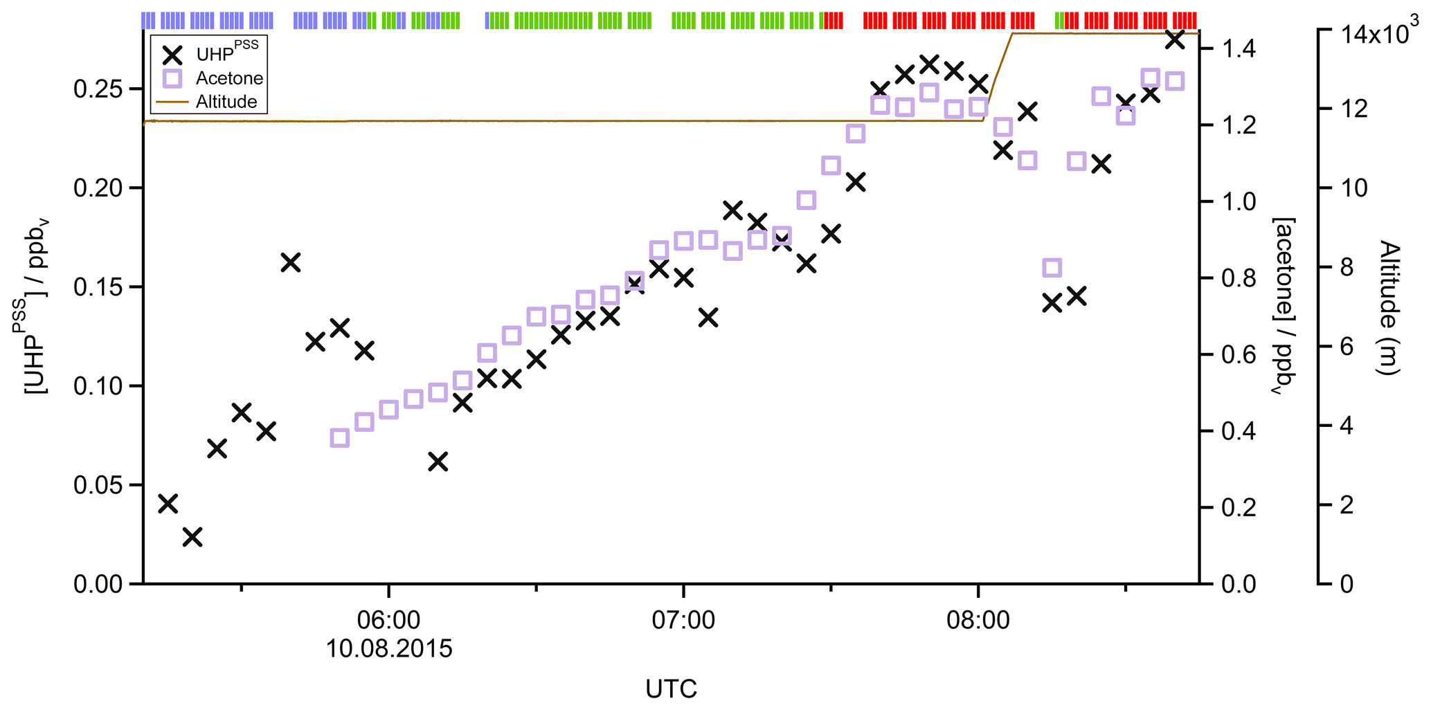
Figure 5 Time series of UHP^PSS (black crosses) and acetone (purple squares) mixing ratios during Flight 17. The brown line shows the altitude, the colored bar on top indicates the origin of air masses according to the methane mixing ratio classification: for SH blue, NH green, and AMA red.

Figure 6 Scatterplots of measured acetone and ${\mathrm{H}}_{\mathrm{2}}{{\mathrm{O}}_{\mathrm{2}}}^{\mathrm{obs}}$ (a), MHP^PSS (b), ROOH^obs (c), and UHP^PSS (d) during Flight 17. The dark purple lines represent the least-orthogonal-distance fits with regression coefficients R² of 0.02, 0.41, 0.43, and 0.82.

Figure 7 Scatterplots of ${\mathrm{H}}_{\mathrm{2}}{{\mathrm{O}}_{\mathrm{2}}}^{\mathrm{obs}}$ (a), ROOH^obs (b), and UHP^PSS (c) and NO∕NO_y ratio during Flight 17.

4.3 Results for the entire campaign

To extend the analysis to the entire campaign, Fig. 8 shows all flight tracks in the UT during OMO. The color code represents observed mixing ratios of ${\mathrm{H}}_{\mathrm{2}}{{\mathrm{O}}_{\mathrm{2}}}^{\mathrm{obs}}$, MHP^PSS, and UHP^PSS varying from low (purple) to high values (red). Histograms for the whole campaign of ${\mathrm{H}}_{\mathrm{2}}{{\mathrm{O}}_{\mathrm{2}}}^{\mathrm{obs}}$ mixing ratios as well as inferred MHP^PSS and UHP^PSS mixing ratios are presented in Fig. 9. Here only data from the UT (<300 hPa, which corresponds to altitudes >9 km) were included in the analysis. Mixing ratios for all species were further differentiated by methane levels such that data in air masses with CH₄ mixing ratios above the threshold of 1879.8 ppb_v were classified as AMA-influenced, while air masses with CH₄ mixing ratios between 1820 ppb_v and 1879.8 ppb_v were classified as NH background and those with CH₄<1820 ppb_v as SH following Tomsche et al. (2019). Figure 9a indicates that ${\mathrm{H}}_{\mathrm{2}}{{\mathrm{O}}_{\mathrm{2}}}^{\mathrm{obs}}$ mixing ratios are most abundant at values of 70–90 ppt_v in NH background air masses (green); 130 to 270 ppt_v with three notable peaks at 180–190, 210–220, and 250–270 ppt_v in SH air masses (blue); and 150–170 ppt_v in AMA-influenced air masses (red). The medians are 115 ppt_v for the NH background, 211 ppt_v for the SH, and 167 ppt_v for the AMA, indicating an excess of 52 ppt_v in AMA-influenced air masses compared to the NH background, while in the SH the ${\mathrm{H}}_{\mathrm{2}}{{\mathrm{O}}_{\mathrm{2}}}^{\mathrm{obs}}$ mixing ratio is twice as high as the NH background. For MHP^PSS (Fig. 9b) the frequency distribution in the NH background shows a maximum at 30–40 ppt_v (green). For AMA-influenced air a sharp maximum at 50–70 ppt_v (red) is found. Air masses from the SH exhibit a rather flat distribution, with a maximum at values of 40–50 ppt_v and a median of 152 ppt_v (blue). With median mixing ratios of 70 and 64 ppt_v, we found only slightly higher mixing ratios for AMA-influenced air masses in comparison to the NH background. For UHP^PSS (Fig. 9c) we again found a flat distribution of mixing ratios in the SH (blue), with a maximum at values of 140–150 ppt_v and a median of 129 ppt_v. The maximum in the frequency distribution for NH background conditions is found at 70–90 ppt_v (green), while in AMA-influenced air masses it was significantly higher, with 210–230 ppt_v (red). Thus, mixing ratios of UHP^PSS are approximately 2–3 times higher in the AMA outflow than in the NH background. This is also represented in the medians of 210 ppt_v in the AMA and 89 ppt_v in the NH background.

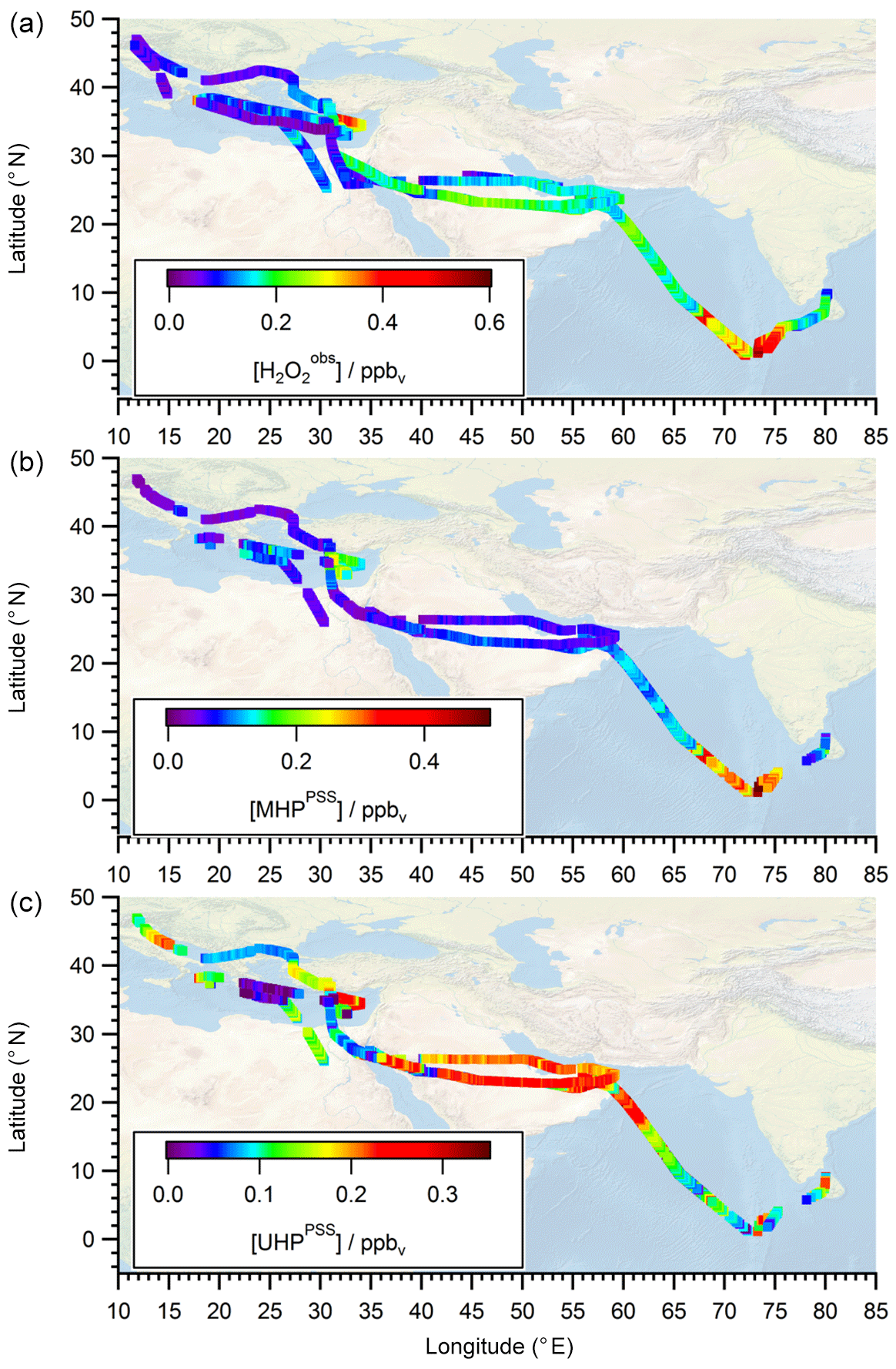
Figure 8 All flight positions in the upper troposphere (p<300 hPa) during OMO as a function of (a) ${\mathrm{H}}_{\mathrm{2}}{{\mathrm{O}}_{\mathrm{2}}}^{\mathrm{obs}}$, (b) MHP^PSS , and (c) UHP^PSS.

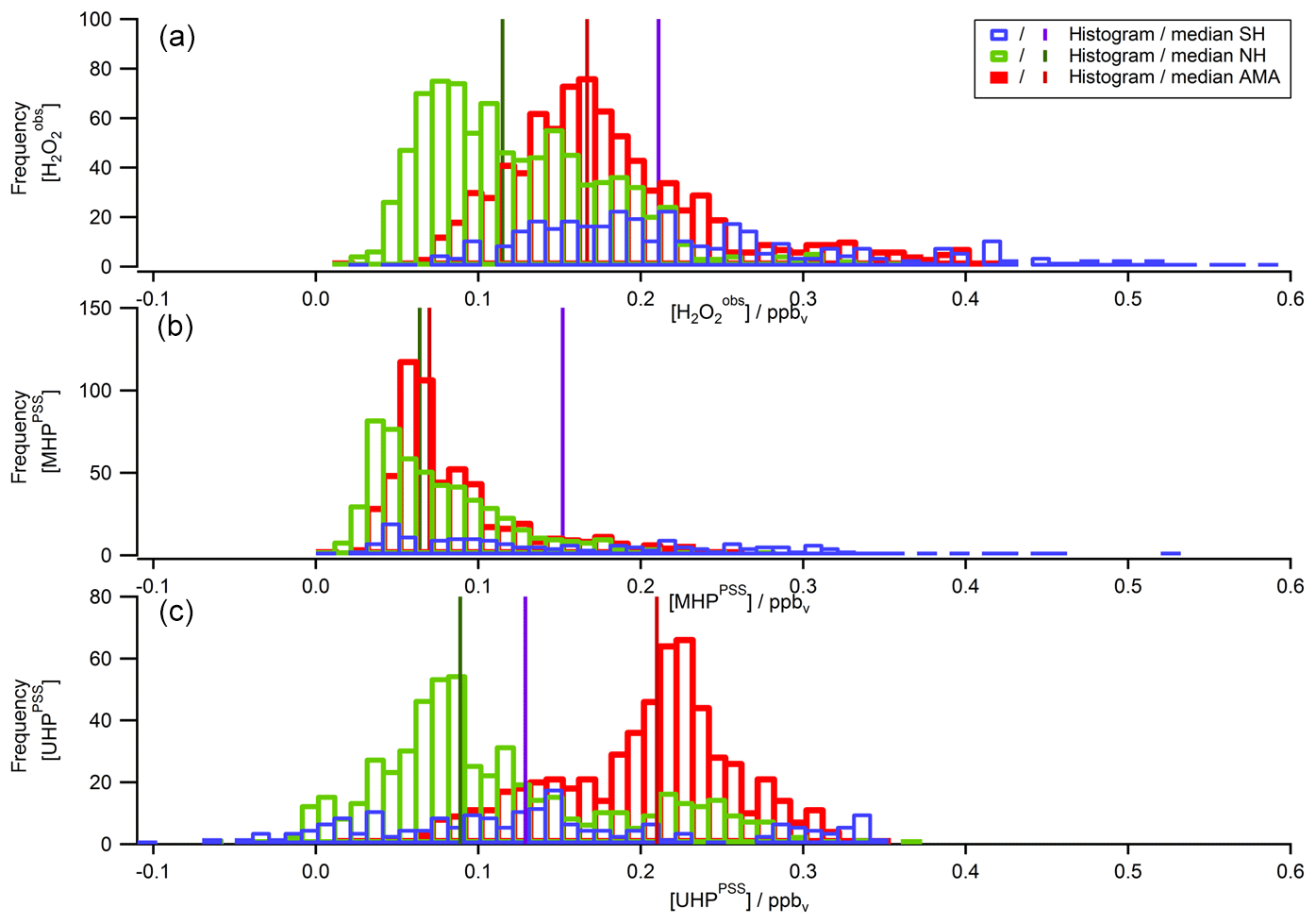
Figure 9 Histograms of ${\mathrm{H}}_{\mathrm{2}}{{\mathrm{O}}_{\mathrm{2}}}^{\mathrm{obs}}$ (a), MHP^PSS (b), and UHP^PSS (c) mixing ratios during the OMO campaign for NH background (green), SH (blue), and AMA (red) air masses.

In the analysis of Flight 17 we found a strong correlation between UHP^PSS and acetone (Fig. 6) and an increase in UHP^PSS at the highest air mass ages, represented by low [NO] ∕ [NO_y] (Fig. 7). Extension of this analysis to all observations in the upper troposphere obtained during OMO yields similar results for the relation between UHP^PSS, ROOH^obs, and ${\mathrm{H}}_{\mathrm{2}}{{\mathrm{O}}_{\mathrm{2}}}^{\mathrm{obs}}$ and acetone (Fig. 10). Enhanced mixing ratios of hydroperoxides are typically associated with enhanced acetone mixing ratios, especially for UHP^PSS. A simple calculation of the production of MHP out of the photolysis of acetone and the reaction of acetaldehyde (from EMAC) with OH shows that per day approximately 40 ppt_v MHP can be formed within the AMA. The lifetime of MHP was calculated to be around 1.5 d. Thus not all of the UHP^PSS in the AMA (median 210 ppt_v) can be accounted for MHP that was chemically produced from VOCs in the AMA. The scatterplots of the hydroperoxides vs. [NO] ∕ [NO_y] for the whole data set show no clear correlation with a large spread of hydroperoxide mixing ratios at the lowest [NO] ∕ [NO_y] ratios, representing the oldest, i.e., chemically most processed, air masses (Fig. 11).

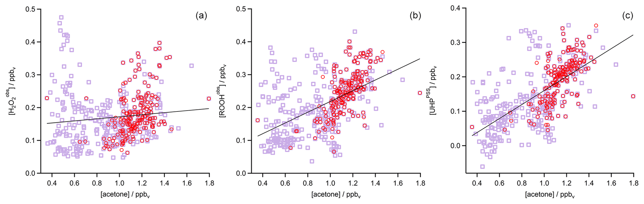
Figure 10 Scatterplots of acetone and ${\mathrm{H}}_{\mathrm{2}}{{\mathrm{O}}_{\mathrm{2}}}^{\mathrm{obs}}$ (a), ROOH^obs (b), and UHP^PSS (c) in the UT (purple squares) and especially in the AMA (red circles). The black lines represent the least-orthogonal-distance fit with linear regression coefficients R² of 0.01 (${\mathrm{H}}_{\mathrm{2}}{{\mathrm{O}}_{\mathrm{2}}}^{\mathrm{obs}}$), 0.27 (ROOH^obs), and 0.41 (UHP^PSS).

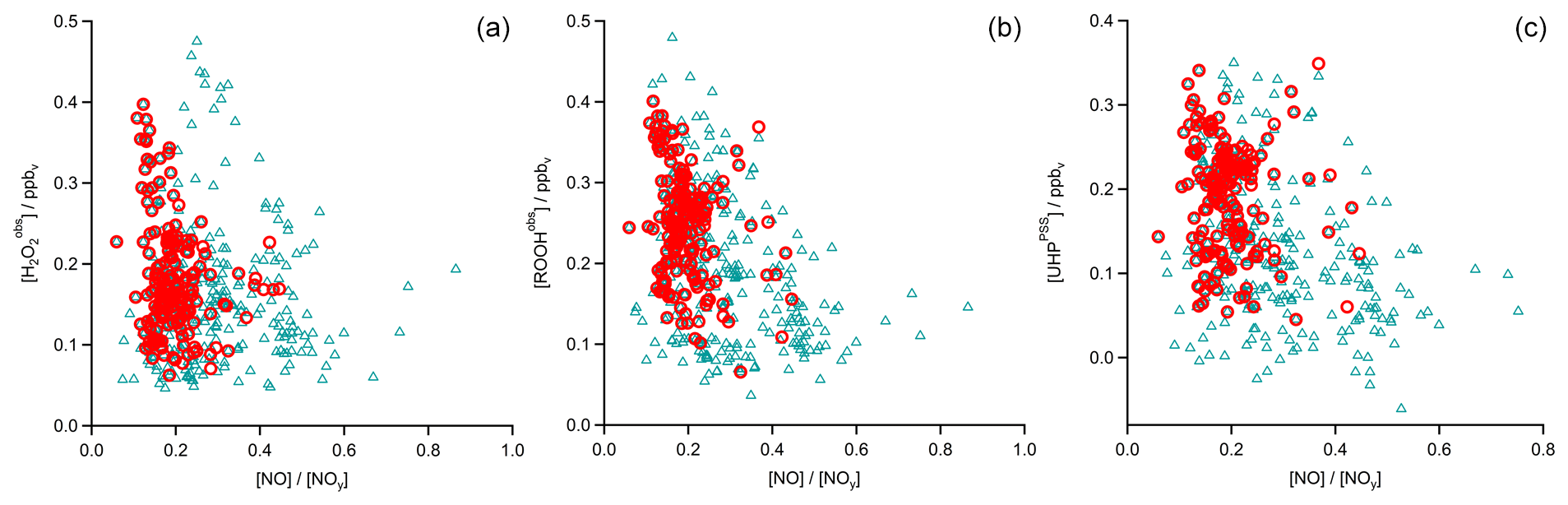
Figure 11 Scatterplots of NO∕NO_y and ${\mathrm{H}}_{\mathrm{2}}{{\mathrm{O}}_{\mathrm{2}}}^{\mathrm{obs}}$ (a), ROOH^obs (b), and UHP^PSS (c) in the UT (blue triangles) and especially in the AMA (red circles).

4.3.1 H₂O₂ steady-state calculation

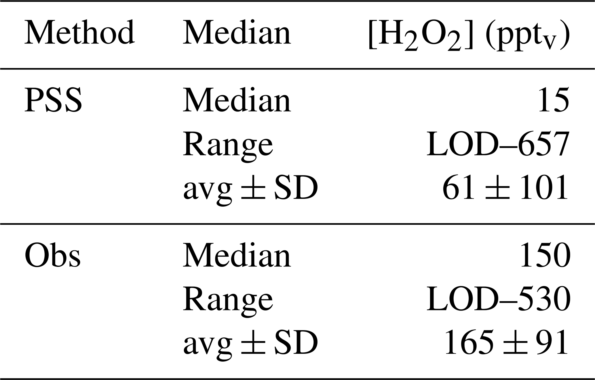
A scatterplot of the results from the ${\mathrm{H}}_{\mathrm{2}}{{\mathrm{O}}_{\mathrm{2}}}^{\mathrm{PSS}}$ based on observed HO_x data in the UT (Eq. 15) is shown in Fig. 12. The dotted black line shows the 1 : 1 line; the dashed green lines represent the 2 : 1 and 1 : 2 relations. It is obvious that the comparison is affected by a rather large offset of approximately 350 ppt_v in the observations that is not accounted for in the steady-state calculations. The regression coefficient R² is 0.26. Most of the ${\mathrm{H}}_{\mathrm{2}}{{\mathrm{O}}_{\mathrm{2}}}^{\mathrm{PSS}}$ mixing ratios (75 %) vary between 0 and 65 ppt_v, with a median value of 15 ppt_v, while the ${\mathrm{H}}_{\mathrm{2}}{{\mathrm{O}}_{\mathrm{2}}}^{\mathrm{obs}}$ mixing ratios extend over a larger range, mainly between 10 and 210 ppt_v, with a median of 150 ppt_v and thus 10 times higher than for steady-state, indicating that more than 80 % of all points in the correlation are outside the range of uncertainty. This can also be seen in the histograms in Fig. 13. Table 1 shows the statistical comparison of both data sets. The discrepancy between ${\mathrm{H}}_{\mathrm{2}}{{\mathrm{O}}_{\mathrm{2}}}^{\mathrm{obs}}$ and ${\mathrm{H}}_{\mathrm{2}}{{\mathrm{O}}_{\mathrm{2}}}^{\mathrm{PSS}}$ shows that the local PSS does not account for all main contributions of H₂O₂ even though all chemical reactions are included. Thus transport phenomena like deep convection seem to play a key role (see Sect. 4.3.3).

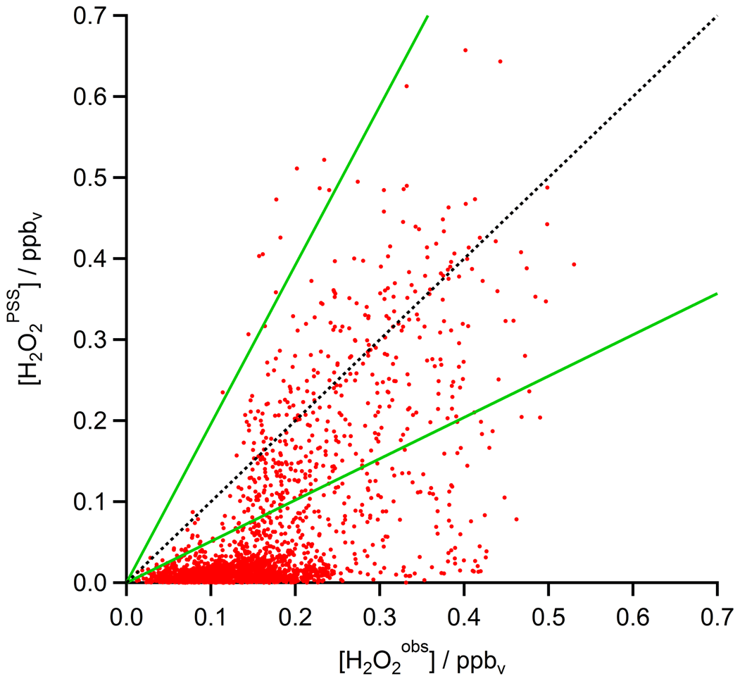
Figure 12 Scatterplot of ${\mathrm{H}}_{\mathrm{2}}{{\mathrm{O}}_{\mathrm{2}}}^{\mathrm{obs}}$ and ${\mathrm{H}}_{\mathrm{2}}{{\mathrm{O}}_{\mathrm{2}}}^{\mathrm{PSS}}$ mixing ratios (red) with the 1 : 1 (black), 1 : 2, and 2 : 1 (both green) lines.

Figure 13 Histograms of ${\mathrm{H}}_{\mathrm{2}}{{\mathrm{O}}_{\mathrm{2}}}^{\mathrm{obs}}$ (a) and ${\mathrm{H}}_{\mathrm{2}}{{\mathrm{O}}_{\mathrm{2}}}^{\mathrm{PSS}}$ (b) mixing ratios (bars) and the associated medians (lines).

Table 1 Comparison of H₂O₂ mixing ratios in the upper troposphere from observations and PSS calculations.

4.3.2 Comparison to EMAC

Figure 14 shows histograms for the comparison between ${\mathrm{H}}_{\mathrm{2}}{{\mathrm{O}}_{\mathrm{2}}}^{\mathrm{obs}}$, MHP^PSS, and UHP^PSS with EMAC simulations. Median ${\mathrm{H}}_{\mathrm{2}}{{\mathrm{O}}_{\mathrm{2}}}^{\mathrm{EMAC}}$ values are similar for NH background (66 ppt_v) and AMA (71 ppt_v) conditions (Table 2), while ${\mathrm{H}}_{\mathrm{2}}{{\mathrm{O}}_{\mathrm{2}}}^{\mathrm{obs}}$ indicate an enhancement of +64 ppt_v in the AMA relative to the NH background. For the SH the model-simulated ${\mathrm{H}}_{\mathrm{2}}{{\mathrm{O}}_{\mathrm{2}}}^{\mathrm{EMAC}}$ (272 ppt_v) mixing ratios are 4 times higher than in the NH background (66 ppt_v), while the ${\mathrm{H}}_{\mathrm{2}}{{\mathrm{O}}_{\mathrm{2}}}^{\mathrm{obs}}$ mixing ratios only show a median increase by roughly a factor of 2 (100 to 211 ppt_v; Table 2).

Figure 14 Histograms of ${\mathrm{H}}_{\mathrm{2}}{{\mathrm{O}}_{\mathrm{2}}}^{\mathrm{obs}}$ and ${\mathrm{H}}_{\mathrm{2}}{{\mathrm{O}}_{\mathrm{2}}}^{\mathrm{EMAC}}$ (a, b), MHP^PSS and MHP^EMAC (c, d), and UHP^PSS and UHP^EMAC (given as PAA^EMAC and EHP^EMAC; e, f) mixing ratios during the OMO campaign for NH background (green), SH (blue), and AMA (red) air masses.

Table 2 Comparison of H₂O₂, MHP and UHP mixing ratios in the upper troposphere from EMAC, measurements and PSS calculations.

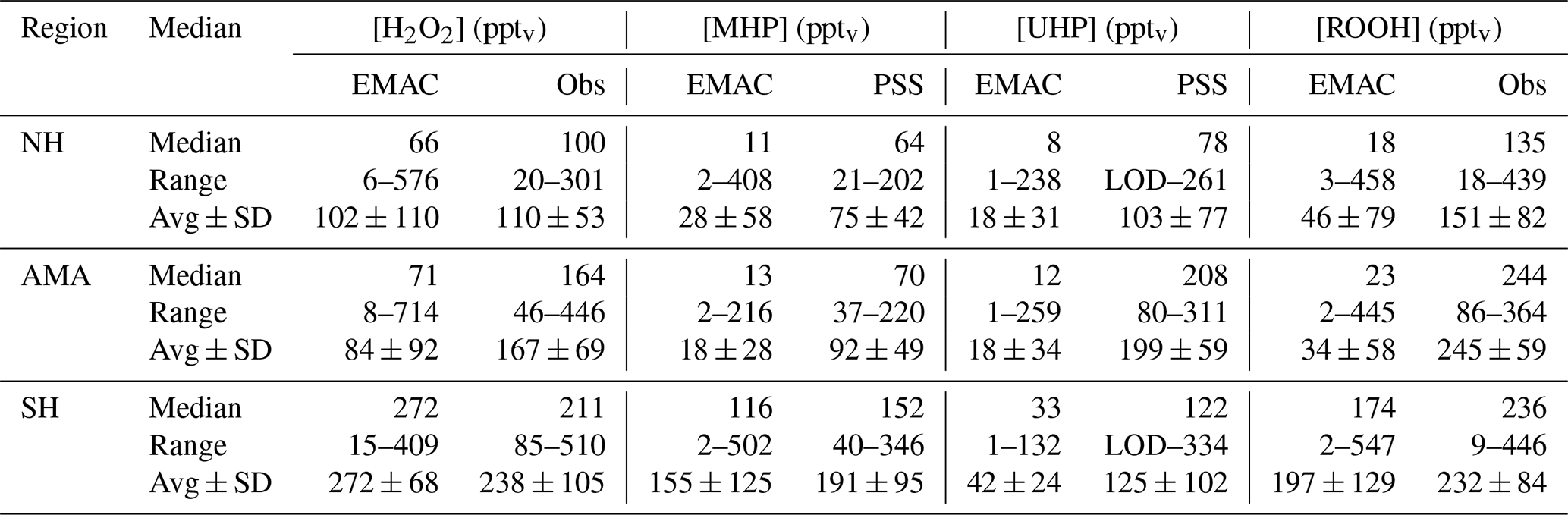
In general EMAC tends to strongly underestimate total hydroperoxide in all air masses by a factor of 5–10. MHP^EMAC mixing ratios are mainly lower than 50 ppt_v for background and AMA, while MHP^PSS ranges from LOD–140 ppt_v. Again the model simulates the highest MHP^EMAC mixing ratios in the SH, with values up to 502 ppt_v compared to up to 346 ppt_v in the MHP^PSS calculations. Similar as for ${\mathrm{H}}_{\mathrm{2}}{{\mathrm{O}}_{\mathrm{2}}}^{\mathrm{EMAC}}$, medians of MHP^EMAC for NH background and AMA conditions show very small differences (11 and 13 ppt_v, respectively; Table 2), while slightly higher differences were found for UHP^EMAC in the AMA (64 and 70 ppt_v, respectively). In the simulations, southern hemispheric MHP^EMAC mixing ratios are almost 10 times higher than NH background values (116 and 11 ppt_v, respectively) compared to 2 to 3 times higher in the observations.

Data for UHP^EMAC in the model are calculated from the sum of simulated ethyl hydroperoxide (EHP) and peroxyacetic acid (PAA), which, according to the model, are the only nonmethyl organic hydroperoxides in the free troposphere with nonzero mixing ratios. UHP^EMAC mixing ratios range from 1 to 238 ppt_v in the NH background, 1 to 259 ppt_v in the AMA, and 1 to 132 ppt_v in the SH. UHP^PSS based on the observations indicate lowest mixing ratios in the NH background (LOD–261 ppt_v), while in the AMA and the SH the ranges are quite similar (80–311 ppt_v and LOD–334 ppt_v). A comparison of median values emphasizes the large difference between model simulations and observation-based estimates. In the NH background, the median UHP^PSS mixing ratio from the observations is 70 ppt_v higher than EMAC simulations (78 and 8 ppt_v, respectively). In the AMA the difference is even larger, with about 200 ppt_v higher UHP^PSS levels compared to the EMAC simulations. The smallest difference, with 89 ppt_v, was found for the SH (Table 2).

4.3.3 Longitudinal gradients

So far discussions of different air masses have been based on measurements of methane, subdividing the observations into NH background, AMA, and SH data. Tomsche et al. (2019) have shown that longitudinal gradients are found in the AMA over the Arabian Peninsula. Observations in the west are often near the edge of the anticyclone, while observations towards the east are closer to its center. In Fig. 16, observations, steady-state calculations, and EMAC simulations for upper tropospheric (9–15 km) H₂O₂ are displayed as a function of longitude from west to east (20–30^∘ N, 36–60^∘ E; according to the red box in Fig. 15). To identify gradients, the data are subdivided into bins of 2^∘ longitude. The observations (orange) show roughly a 100 % increase in ${\mathrm{H}}_{\mathrm{2}}{{\mathrm{O}}_{\mathrm{2}}}^{\mathrm{obs}}$ from west to east (90 to 175 ppt_v), similar to simulation with EMAC (black), although absolute mixing ratio levels in ${\mathrm{H}}_{\mathrm{2}}{{\mathrm{O}}_{\mathrm{2}}}^{\mathrm{EMAC}}$ are smaller (61 to 121 ppt_v). Contrary to these observed gradients, ${\mathrm{H}}_{\mathrm{2}}{{\mathrm{O}}_{\mathrm{2}}}^{\mathrm{PSS}}$ mixing ratios based on HORUS data (blue) do not vary with longitude, except for the last two bins. The steady-state calculations are based exclusively on observed concentrations of HO₂ and OH radicals and thus yield only the net photochemical production, while the EMAC simulations and the observations will also account for vertical and horizontal advection from upwind source regions. Previous studies show inconsistent results. Snow et al. (2007) and Barth et al. (2016) for example both show that H₂O₂ is depleted in convective outflow compared to background upper troposphere. In contrast, other studies found that deep convection can be a source of H₂O₂ in the upper troposphere (e.g., Jaeglé et al., 1997; Prather and Jacob, 1997; Mari et al., 2003; Bozem et al., 2017). Similarly, convection over India during the summer monsoon is a potential source of excess H₂O₂ in the upper troposphere. With a photochemical lifetime of several days, this excess in H₂O₂ reaches the western AMA, giving rise to the observed and model-simulated longitudinal gradients. Since the steady-state calculations do not account for transport, this can explain the rather large deviation of 144–164 ppt_v (between 51 and 57^∘) from the observations. Differences between observation and EMAC simulation could potentially arise due to uncertainties in the scavenging efficiency for H₂O₂ as the chemistry does not seem to be a dominant cause of uncertainty.

Figure 15 Location of measurements used for the longitudinal gradient study (red box) out of all flight tracks (black).

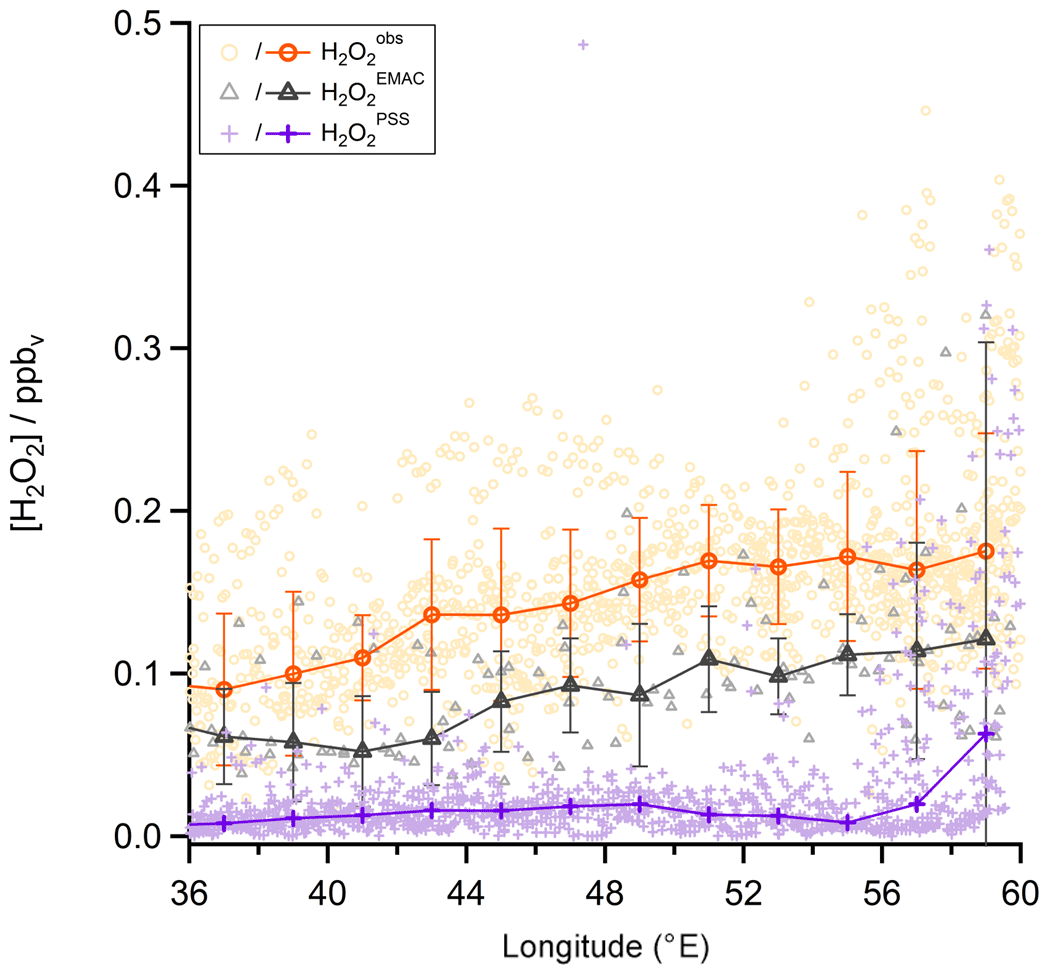
Figure 16 Longitudinal trends of ${\mathrm{H}}_{\mathrm{2}}{{\mathrm{O}}_{\mathrm{2}}}^{\mathrm{obs}}$ mixing ratios (orange circles), ${\mathrm{H}}_{\mathrm{2}}{{\mathrm{O}}_{\mathrm{2}}}^{\mathrm{EMAC}}$ (black triangles), and ${\mathrm{H}}_{\mathrm{2}}{{\mathrm{O}}_{\mathrm{2}}}^{\mathrm{PSS}}$ (purple plus signs). The data are shown in the light colors while the darker ones represent the medians.

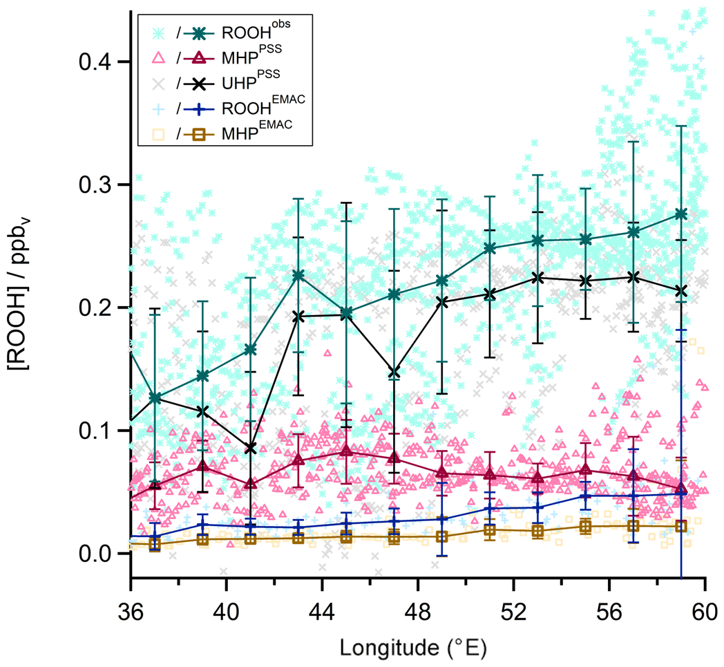
Figure 17 Longitudinal trends of ROOH^obs mixing ratios (green asterisks), ROOH^EMAC (blue plus signs), and mixing ratios for MHP^PSS (pink triangles) and UHP^PSS (black crosses) as well as MHP^EMAC (yellow squares). The data are shown in the light colors, while the darker ones represent the medians.

Similar longitudinal gradients are also observed for measured total organic hydroperoxides (ROOH^obs; green asterisks in Fig. 17), inferred UHP^PSS (black); and total ROOH^EMAC (blue). Steady-state calculations of MHP^PSS (pink) and simulations of MHP^EMAC (yellow) show either no or only weak longitudinal gradients. Assuming that MHP is also enhanced in the outflow of deep convection (Mari et al., 2000; Barth et al., 2016), at least part of the enhancement in ROOH^obs (and thus inferred UHP^PSS) could be due to advected MHP.

4.4 Discussion

To our knowledge we present the first observations of H₂O₂ and ROOH mixing ratios in the Asian monsoon anticyclone. Previous studies have been mainly focused on the northern hemispheric upper troposphere. Several aircraft campaigns including peroxide measurements were performed over North America. They are summarized in Snow et al., 2007): the SONEX campaign took place in fall 1997 in the UT and yielded mean values of 120 ppt_v for H₂O₂ and 50 ppt_v for MHP (medians: 80 and 30 ppt_v, respectively). The TOPSE campaign in winter/spring 2000 probed the middle troposphere, yielding median H₂O₂ and MHP mixing ratios of 150 ppt_v for both species. During the INTEX-NA campaign in summer 2004, observed median mixing ratios at altitudes of 6–10 km were about 400 ppt_v for H₂O₂ and 200 ppt_v for MHP. A comparison with our results (Table 2) shows that we found similar mixing ratios as in SONEX in the northern hemispheric background of 115 and 64 ppt_v for H₂O₂ and MHP, respectively. Mixing ratios for both species reported for TOPSE and INTEX-NA are slightly higher than ours, which may be related to the lower altitude range of 6–10 km (in comparison to >9 km for OMO) in these studies. Previous observations have shown that H₂O₂ and MHP show the highest mixing ratios at altitudes between 2 and 5 km followed by a sharp decrease towards higher altitudes (see e.g., Daum et al., 1990; Heikes, 1992; Weinstein-Lloyd et al., 1998; Snow, 2003; Snow et al., 2007; Klippel et al., 2011).

Heikes et al. (1996) associated enhanced H₂O₂ mixing ratios above 5 km in the North Pacific of the Asian coast (30^∘ N) with outflow from Typhoon Mireille (Heikes et al., 1996). These observations were made close to the source region for the AMA-influenced air masses described here (see back trajectories in the case study of Flight 17; Fig. 2 or Tomsche et al., 2019). For MHP Heikes et al. (1996) found mixing ratios of 250–500 ppt_v in the southern longitudinal section above 5 km, similar to median mixing ratios of 152 ppt_v for MHP in SH air masses in the UT found in this study.

Although the mixing ratios observed during this study are similar to previous observations in the upper troposphere, one striking result is that a state-of-the-art global circulation model (EMAC) and a local steady-state calculation constrained by measured radical levels significantly underestimate H₂O₂ mixing ratios in particular in the AMA. The general tendency is that the steady-state model produces the lowest values, with EMAC falling in between steady state and observations (e.g., Fig. 16). A comparison of the EMAC simulations for the two radicals that affect H₂O₂ most strongly (OH and HO₂) yields a rather good agreement. A scatterplot between modeled and observed HO₂ yields a slope of 0.72±0.01 (ppt_v ppt_v⁻¹) and an offset of 4.30±0.09 ppt_v, with a regression coefficient R² of 0.58 (Fig. 18 left). The OH data show more scatter, with a tendency for EMAC to overestimate the mixing ratios (slope: 1.7±0.2 (ppt_v ppt_v⁻¹); offset: $-\mathrm{0.1}\pm \mathrm{0.1}$ ppt_v; regression coefficient R²: 0.09; Fig. 18 right). Although there is rather good agreement between EMAC simulations and observations for all the species that affect the local photochemical budget of H₂O₂, EMAC significantly exceeds PSS calculation for H₂O₂. This is an indication that an additional H₂O₂ source is accounted for in the global model and that the local photostationary-state assumption is not fulfilled. The additional source is attributed to transport associated with deep convection over India, yielding an upwind source of H₂O₂ that is significant throughout the western part of the AMA. In the AMA, clouds are absent so that gas-phase photochemical processes may determine the lifetime of H₂O₂. Based on observed OH^obs levels and photolysis frequencies during OMO, the H₂O₂ lifetime in the upper troposphere is of the order of several days, sufficiently long for the excess H₂O₂ to reach the western parts of the AMA, producing the observed longitudinal H₂O₂ gradient observed in both observations and EMAC simulations (Fig. 16). The total amount of H₂O₂ injected into the UT by convective outflow depends on the scavenging efficiency (Mari et al., 2000; Barth et al., 2016; Bozem et al., 2017). Differences between ${\mathrm{H}}_{\mathrm{2}}{{\mathrm{O}}_{\mathrm{2}}}^{\mathrm{obs}}$ and ${\mathrm{H}}_{\mathrm{2}}{{\mathrm{O}}_{\mathrm{2}}}^{\mathrm{EMAC}}$ are most likely due to an overestimation of scavenging in the model as also pointed out by Klippel et al., 2011).

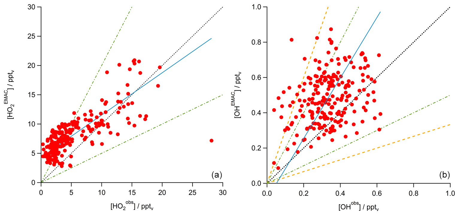
Figure 18 Scatterplot of ${{\mathrm{HO}}_{\mathrm{2}}}^{\mathrm{obs}}$ and ${{\mathrm{HO}}_{\mathrm{2}}}^{\mathrm{EMAC}}$ data (a) and OH^obs and OH^EMAC data (b; both red) with the 1 : 1 (black), 1 : 2, and 2 : 1 (both green) lines. The blue line shows the calculated least-orthogonal-distance fit.

To investigate this assumption we performed a sensitivity study with the wet scavenging for all soluble species being switched off globally. The result is shown in Fig. 19. The ${\mathrm{H}}_{\mathrm{2}}{{\mathrm{O}}_{\mathrm{2}}}^{\mathrm{EMAC}}$ mixing ratios significantly increase with longitude by a factor of 3–4 and thus to the level of ${\mathrm{H}}_{\mathrm{2}}{{\mathrm{O}}_{\mathrm{2}}}^{\mathrm{obs}}$. Please note that significant enhancements in MHP^EMAC and ROOH^EMAC were not found in the sensitivity study with switched-off scavenging, indicating that the strong underestimation by the model of these species is not due to an overestimation of wet removal in convective clouds. Instead, we found that EMAC underestimates ROOH in all air masses and not only in the AMA. The reasons for this underestimation are unknown. In a previous comparison of MHP observations and EMAC simulations over Europe for July 2007, Klippel et al. (2011) also reported a difference of a factor of 10 in the upper troposphere, while a comparison during the fall season (October 2006) yielded a rather good agreement (within a factor of 2).

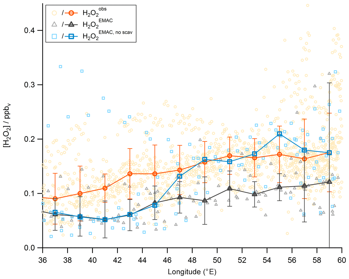
Figure 19 Longitudinal trends of ${\mathrm{H}}_{\mathrm{2}}{{\mathrm{O}}_{\mathrm{2}}}^{\mathrm{obs}}$ mixing ratios (orange circles), ${\mathrm{H}}_{\mathrm{2}}{{\mathrm{O}}_{\mathrm{2}}}^{\mathrm{EMAC}}$ (black triangles), and the sensitivity study without scavenging in ${\mathrm{H}}_{\mathrm{2}}{{\mathrm{O}}_{\mathrm{2}}}^{\mathrm{EMAC}}$ (blue circles). The data are shown in the light colors, while the darker ones represent the medians.

There is a rather large uncertainty regarding the scavenging efficiency of MHP in deep convection (Barth et al., 2016). For the Trace A campaign Mari et al. (2000) found observed (modeled) enhancement ratios of postconvective mixing ratios in comparison to preconvective mixing ratios of 11 (9.5) for MHP and 1.9 (1.2) for H₂O₂. Such efficient transport in the Indian summer monsoon would yield a strong source of upper-tropospheric MHP, explaining the large enhancement of ROOH^obs in the AMA described here. Please note that large enhancements of MHP^EMAC and ROOH^EMAC were not found in the sensitivity study with switched-off scavenging, indicating that the strong underestimation by the model of those species is not due to an overestimation of wet removal in convective clouds. It seems that a large part of the UHP^PSS is actually MHP advected throughout the AMA after deep convective transport over India. In the EMAC simulations the transport of MHP is less efficient, and thus MHP^EMAC is lower than MHP^PSS and UHP^PSS. Please note that EMAC has a general tendency to overestimate CO in the UT, especially for the NH background, while it tends to underestimate CH₄ (Tomsche et al., 2019). The deviations in general are not significant, with the exception of CH₄ in the AMA (Table 1 in Tomsche et al., 2019). As discussed in Tomsche et al. (2019), the CH₄ mixing ratio in the AMA depends of the colocation of convection and underlying methane sources. The model resolution of 2.8^∘ × 2.8^∘ is not sufficient to resolve small-scale variations in both convection and CH₄ source distribution. The H₂O₂ mixing ratio over the Indian subcontinent is not expected to show large spatial variations since latitudinal gradients are generally small (see, e.g., Klippel et al., 2011). Therefore, we do not expect that the model resolution will have a strong influence on the deviation between ${\mathrm{H}}_{\mathrm{2}}{{\mathrm{O}}_{\mathrm{2}}}^{\mathrm{obs}}$ and ${\mathrm{H}}_{\mathrm{2}}{{\mathrm{O}}_{\mathrm{2}}}^{\mathrm{EMAC}}$. Another uncertainty arises from missing information on the absolute mixing ratios of H₂O₂, MHP, and higher organic hydroperoxides in the inflow region of deep convection over India since observations of these species in the boundary layer over India are not available. Note that the amount of hydrogen peroxide and number of organic hydroperoxides transported to the upper troposphere depends on the scavenging efficiency and on the mixing ratios of the individual species in the inflow region (Barth et al., 2016; Bozem et al., 2017). Thus, an underestimation of hydroperoxides in the upper troposphere after convective injection can be due either to an underestimation of the scavenging efficiency for individual species, an underestimation of their mixing ratio in the inflow region, or a combination of both and might differ for individual hydroperoxides. Due to a lack of observations in the inflow and outflow region of convection over India, this question cannot be resolved in this study.

5 Conclusions

Hydrogen peroxide and organic hydroperoxides were measured during the OMO campaign in the upper troposphere in NH background air over the western Mediterranean, the Asian summer monsoon anticyclone over the Arabian Peninsula, and the SH over the Maldives and the Indian Ocean in summer 2015. The observed mixing ratios for background conditions in the NH and SH are in line with previous studies described in the literature. A case study (of Flight 17) revealed enhanced ${\mathrm{H}}_{\mathrm{2}}{{\mathrm{O}}_{\mathrm{2}}}^{\mathrm{obs}}$ and ROOH^obs mixing ratios in the AMA relative to the NH background. Similar results are found for other flights throughout the campaign. The atmospheric chemistry general circulation model EMAC slightly underestimates ${\mathrm{H}}_{\mathrm{2}}{{\mathrm{O}}_{\mathrm{2}}}^{\mathrm{EMAC}}$ in the NH background (medians: 66 ppt_v vs. 100 ppt_v), significantly underestimates it in the AMA (medians: 71 ppt_v vs. 164 ppt_v), and overestimates it in the SH (medians: 272 ppt_v vs. 211 ppt_v). Steady-state calculations for ${\mathrm{H}}_{\mathrm{2}}{{\mathrm{O}}_{\mathrm{2}}}^{\mathrm{PSS}}$ and MHP^PSS based on observed precursors yield much lower values compared to ${\mathrm{H}}_{\mathrm{2}}{{\mathrm{O}}_{\mathrm{2}}}^{\mathrm{obs}}$ and MHP^PSS by roughly a factor of 3, in particular in the AMA, resulting in a large contribution of an unidentified organic hydroperoxide (UHP^PSS) in air masses affected by the AMA. A comparison between EMAC simulations and HO_x levels shows a good agreement, indicating that deviations between ${\mathrm{H}}_{\mathrm{2}}{{\mathrm{O}}_{\mathrm{2}}}^{\mathrm{EMAC}}$ and ${\mathrm{H}}_{\mathrm{2}}{{\mathrm{O}}_{\mathrm{2}}}^{\mathrm{PSS}}$ levels are due to transport. Convective injection of H₂O₂ (and ROOH) into the upper troposphere over India most likely forms a pool of hydroperoxides in the upper troposphere that subsequently influences the western AMA, giving rise to a significant longitudinal gradient of H₂O₂ and ROOH mixing ratios, with increasing values towards the center of the AMA. It is likely that next to an unidentified organic hydroperoxide (e.g., PAA), at least part of UHP^PSS is due to additional MHP from an upwind source. A sensitivity study using EMAC with no scavenging tends to reproduce the observed longitudinal gradients in H₂O₂, although it does not increase the level of ROOH. The reasons for this different behavior are unclear.