the Creative Commons Attribution 4.0 License.
the Creative Commons Attribution 4.0 License.
 | 03 Nov 2020
Linkage among ice crystal microphysics, mesoscale dynamics, and cloud and precipitation structures revealed by collocated microwave radiometer and multifrequency radar observations
Xiping Zeng
Dong L. Wu
S. Joseph Munchak
Xiaowen Li
Stefan Kneifel
Davide Ori
Liang Liao
Donifan Barahona
Ice clouds and falling snow are ubiquitous globally and play important roles in the Earth's radiation budget and precipitation processes. Ice particle microphysical properties (e.g., size, habit and orientation) are not only influenced by the ambient environment's dynamic and thermodynamic conditions, but are also intimately connected to the cloud radiative effects and particle fall speeds, which therefore have an impact on future climate projection as well as on the details of the surface precipitation (e.g., onset time, location, type and strength).
Our previous work revealed that high-frequency (> 150 GHz) polarimetric radiance difference (PD) from passive microwave sensors is a good indicator of the bulk aspect ratio of horizontally oriented ice particles that often occur inside anvil clouds and/or stratiform precipitation. In this current work, we further investigate the dynamic and thermodynamic mechanisms and cloud–precipitation structures associated with ice-phase microphysics corresponding to different PD signals. In order to do so, collocated CloudSat radar (W-band) and Global Precipitation Measurement Dual-frequency Precipitation Radar (GPM DPR, Ku–Ka-bands) observations as well as European Centre for Medium-Range Weather Forecasts (ECMWF) atmosphere background profiles are grouped according to the magnitude of PD for only stratiform precipitation and/or anvil cloud scenes. We found that horizontally oriented snow aggregates or large snow particles are likely the major contributor to the high-PD signals at 166 GHz, while low-PD magnitudes can be attributed to small cloud ice, randomly oriented snow aggregates, riming snow or supercooled water. Further, high-PD (low-PD) scenes are found to be associated with stronger (weaker) wind shear and higher (lower) ambient humidity, both of which help promote (prohibit) the growth of frozen particles and the organization of convective systems. An ensemble of squall line cases is studied at the end to demonstrate that the PD asymmetry in the leading and trailing edges of the deep convection line is closely tied to the anvil cloud and stratiform precipitation layers, respectively, suggesting the potential usefulness of PD as a proxy of stratiform–convective precipitation flag, as well as a proxy of convection life stage.
- Article
(11470 KB) - Full-text XML
- BibTeX
- EndNote


Ice clouds and falling snow are ubiquitous. It is found that on average 50 % of the surface precipitation globally is linked to ice in clouds either through the production of snow from ice crystals or through melting of ice into rain (Field and Heymsfield, 2015). While the primary driver of precipitation amounts is determined by the amount of water vapor available to condense and the forcing mechanism, ice microphysical processes play a key role in determining how much, and where, precipitation reaches the ground. For example, ice fall speed is closely tied to the frozen particle habit (i.e., shape), size, density, orientation, etc., and can hence influence the spatial and temporal distributions of precipitation (Milbrandt and Yau, 2006). Studies also show that ice cloud radiative effect (CRE) is strongly dependent on ice microphysical properties (Liou et al., 2002; Tang et al., 2017; Zeng et al., 2009a, b). Therefore, it is critically important to measure, understand and appropriately incorporate ice microphysical properties in models in order to accurately capture the spatial and temporal variations in ice clouds, falling snow and surface precipitation for the sake of improving weather prediction and climate projection.
Due to the complexity and multifaceted characteristics of ice microphysics measurements, multifrequency radar and polarimetric radar are probably the best choices from the remote sensing point of view. For radar frequencies in millimeter to sub-millimeter regimes whose wavelengths are comparable in size to large ice to precipitating particles, the strong scattering signals and their amplitude differences at different wavelengths can provide ample information about vertical profiles of frozen particle density, particle size distribution (PSD), phase, etc. (Kneifel et al., 2011, 2015, 2016; Kulie et al., 2014; Dias Neto et al., 2019). Triple-frequency radar measurement techniques have been gaining attention and developed quickly in the past decade, and they have been implemented at some research ground stations or field campaigns (e.g., Chase et al., 2018). Polarimetric radar (or dual-polarization radar) measures radio wave pulses that are horizontally and vertically polarized at the same frequency. Their reflectivity difference (ZDR) and specific differential phase (KDP) can help better constrain the retrieval of precipitation intensity and phase discrimination (Simmons and Sutter, 2005).
Although active radar measurements are superb in revealing ice microphysical properties, their availability from space is limited to a curtain or narrow swaths due to mass, power and data transfer requirements. Although many ongoing efforts are pushing small-payload spaceborne radars such as RainCube Ka-band radar into space, their sensitivity, stability and reliability still require further improvements. Currently in space only CloudSat W-band radar (and EarthCARE W-band radar as a successor to be launched in the near future) and Global Precipitation Measurement (GPM) Dual-frequency Precipitation Radar (DPR, Ku- and Ka-bands) are operating on a regular basis, unprecedentedly deepening our understanding of ice microphysical characteristics globally (Stephens et al., 2002; Luo et al., 2008; Gettelman et al., 2010; Skofronick-Jackson et al., 2018). However, their spatial and temporal coverages are still extremely limited (see instrument specifications in Sect. 2). Besides, the near-nadir views are not conducive for polarimetric measurements of ice properties.
Satellite-borne passive microwave sensors with channels suitable for measuring hydrometers have been continuously monitoring Earth's weather for more than 30 years (Manaster et al., 2017). High-frequency microwave channel (frequency > 150 GHz) signals are dominated by frozen particle scattering when relatively thick ice clouds or frozen precipitation are present along the line of sight and are hence ideal for retrieving bulk ice cloud properties such as ice water path (IWP) (Gong and Wu, 2014; Eriksson et al., 2015). Although not available on geostationary platforms, currently there are more than 10 operating polar-orbiting or procession-orbiting passive microwave sensors with channels beyond 150 GHz (NASA Goddard Space Flight Center PPS and GPM Intercalibration Working Group, 2017). With swath width typically over 1000 km and a footprint size of 7–15 km, their combined usage can readily generate ice hydrometer products on temporal and spatial scales that suit the needs of both weather and climate studies.
Physically based hydrometer retrieval algorithms are widely used to interpret the data from passive microwave sensors. In these algorithms, ice cloud profiles are estimated by accounting for the radiative transfer through frozen or liquid hydrometers as well as gas absorbers before reaching the complicated surfaces with a wide range of emissivity (e.g., Wu and Jiang, 2004 for Microwave Limb Sounder; NOAA MIRS 1D-Var retrieval system). While some of the recent products have advanced from using spherical ice models to more realistic habits (e.g., MODIS Collection 6 assumed a bulk column-aggregate shape globally for its ice cloud property retrieval, Platnick et al., 2017; GPM products assume nonspherical but randomly oriented ice in version 6, Ringerud et al., 2019), random orientation is still nearly always assumed to avoid the complexity of deriving size and orientation simultaneously, as well as to avoid solving equations for four Stokes parameters simultaneously. Ancillary data such as temperature profiles are often needed as well. To overcome these shortcomings, efforts have been put forward to use spaceborne active sensor information to help improve or constrain the error bar of the ice hydrometer retrieval products from passive microwave sensors (e.g., Evans et al., 2012; Gong and Wu, 2014). In particular, the GPM team uses DPR-retrieved hydrometer vertical profiles as either the a priori database or “training” datasets to generate their official passive microwave and joint retrieval products (Kummerrow et al., 2015; Turk et al., 2018).
Among currently available spaceborne high-frequency microwave sensors, the GPM Microwave Imager (GPM GMI) has a unique vertically polarized (V-pol) and horizontally polarized (H-pol) channel pair at 166 GHz. Gong and Wu (2017) found that the magnitude of 166 GHz polarization difference (PD), defined as the brightness temperature (TB) difference between V-pol and H-pol (PD ≡ TBV–TBH), is a good indicator of the presence of oriented ice particles. The largest PDs are found in moderately cold TB (∼ 200K), corresponding to predominately horizontally oriented ice or snow particles inside medium thick ice cloud (e.g., anvils) or the stratiform precipitation layer. This feature was also identified from 85 GHz TMI (Tropical Rainfall Measuring Mission's Microwave Imager) measurements (Prigent et al., 2005) and 157 GHz MADRAS (Megha-Tropiques' Microwave Analysis and Detection of Rain and Atmospheric Structures) measurements (Defer et al., 2014). In particular, Olson et al. (2011) used TMI 89 GHz PD as one of the several parameters for stratiform and convective precipitation classification. PD approaches zero for clear-sky and deep convective cores. For the former, this is because 166 GHz is not sensitive to surface polarization when column water vapor exceeds abut 20 mm (Zeng et al., 2019; Munchak et al., 2020). As for the latter, Gong and Wu (2017) provided several possible explanations, including random orientation of ice particles induced by the turbulent environment inside deep convective cores, large irregular-shaped graupel, or both V-pol and H-pol reach saturation at the same optical depth. Gong et al. (2017) further found that PD has a strong diurnal cycle over tropical land that is opposite to the diurnal cycle of cloud thickness and surface precipitation rate. The diurnal cycle of PD leads the latter two by ∼ 2 h, indicating that ice microphysics change over the convection life cycle, which is important to the final precipitation received at the ground. Nevertheless, all of the aforementioned papers studied passive sensor signals only. Scattering signals from passive sensors have very limited information on the vertical distribution of ice particles and hence did not answer some fundamental questions: which altitude does PD information come from? What microphysical and environmental factors affect the observed PD variation over time and space? Can PD give more information in a broader context rather than just microphysics? In this paper, these questions will be addressed by utilizing collocated GMI, DPR and CloudSat radar measurements as well as auxiliary environment variables.
This paper is organized as follows. Section 2 will introduce the dataset and methodology we use to make the composites of climatology. We will present in Sect. 3 the differences of radar reflectivity, temperature and water vapor between high- and low-PD scenes. In Sect. 4, we will thoroughly discuss the underlying physical and microphysical mechanisms as well as consequences of such discrepancies. In Sect. 5, an ensemble of 47 squall line cases will be presented to showcase the potential use of high-frequency passive microwave PD observations to differentiate precipitation system life stage. Section 6 summarizes the whole work and points out several future study directions.
2.1 GPM core satellite and definition of PD regimes
The Global Precipitation Measurement (GPM) mission core satellite, launched on 27 February 2014, carries the Dual-Frequency Precipitation Radar (DPR) and the GPM Microwave Imager (GMI). The GPM core satellite flies at an altitude of 407 km in a precessing orbit covering the Earth at 65∘ S to 65∘ N. DPR is composed of a Ku-band radar (KuPR) and a Ka-band radar (KaPR), making measurements at 13.6 and 35.5 GHz, respectively. DPR scans cross-track with a footprint size of ∼ 5 km × 5 km at nadir and a swath width of 245 km for KuPR and 120 km for KaPR, respectively. Both KuPR and KaPR shoot 49 beams in each scan with a range resolution of 250 m (oversampled to 125 m), but 25 KaPR beams are matched with KuPR footprints for the dual-frequency algorithm to work, and the remaining 24 beams are in interlaced mode with a range resolution of 250 m. Therefore, there are total three modes of DPR scanning pattern: normal scan by KuPR (NS), matched scan by KaPR (MS) and high-resolution interlaced scan by KaPR (HS)1. In this paper, we will mainly use KuPR measurements, and the central-25 MS measurement is used whenever “KaPR” is mentioned. The 2A.GPM.DPR version 05A reflectivity without attenuation correction is used in this study. More mission details can be found at Skofronick-Jackson et al. (2018, 2019) and the GPM website at https://gpm.nasa.gov/, last access: 29 October 2020.
GMI is a 13-channel conical-scan microwave radiometer that sweeps the forward-looking cone at 48.5∘ (Earth incident angle of 52.8∘) from 10 to 89 GHz and at 45∘ (Earth incident angle of 49.2∘) from 166 to 183 GHz. Only the 166 GHz V-pol and H-pol measured brightness temperature (1B.GPM.GMI, version 05A) will be considered in the current paper (TBV and TBH, respectively, hereafter). The 166 GHz footprint size is 7.2 km × 4.2 km (cross-track and along-track), and at this frequency the swath width is 885 km on the Earth's surface in the cross-track direction with 221 pixels in each scan, the center part of which overlays with DPR scan during each GMI scan (https://pmm.nasa.gov/gpm/flight-project/gmi, last access: 29 October 2020).
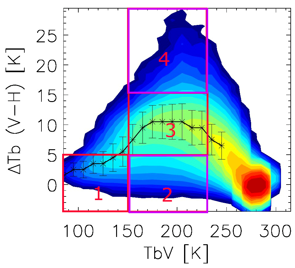
Figure 1The definition of PD regimes according to the TBv and PD values: (1) deep convective, (2) low PD, (3) medium PD and (4) high PD. See text for values regarding the regime definition. Regimes (2) low PD and (4) high PD, enclosed by purple rectangles, are the focus of study in this current work. Two-dimensional PDF contours are adapted from Fig. 3 of Gong and Wu (2017).
Gong and Wu (2017) constructed the two-dimensional probability density function (PDF) for the PD–TBv relationship for different latitude ranges; one example is shown in Fig. 1 for the deep tropics (5∘S–Equator). PD has a large spread when TB is in the middle of the observed range, implying different cloud and precipitation regimes are likely embedded in this moderately cold TB regime, which would be impossible to separate if TBv is the only metric to consider. For simplicity, we arbitrarily define four regimes in Fig. 1: regime 1 (TB <150 K, PD <5 K) represents deep convective scenes (called “deep convective regime” hereafter); regimes 2, 3 and 4 share the same TB bounds (150 K < TB < 230 K) but different PD ranges, namely “low-PD” (PD <5 K), “medium-PD” (5 K < PD < 15 K) and “high-PD” (PD < 15 K) regimes. Of course, these thresholds are arbitrary, but those thresholds based on TBs are consistent with previous literature. For example, TB166 GHz<150 K is roughly equivalent to TB85 GHz<220 K that was previously employed by Nesbitt et al. (2000). This paper will focus on the differences between low-PD and high-PD regimes, as one can imagine that the situations falling in the medium-PD regime must be in transition status between the low-PD and high-PD scenarios. Since the general characteristics of the PD–TBv relationship are largely latitude-independent (Gong and Wu, 2014), this four-regime definition can be applied globally to all GMI measurements, except there are much fewer observations falling into the deep convective regime at high latitudes. Besides, shallow convection that is not as thick as deep convective cloud (e.g., congestus) may be wrongly classified into the low-PD regime. However, as the total congestus area is much smaller than anvil/stratiform precipitation areas (e.g., Zeng et al., 2018), the immixture of shallow convection structures should have a negligible impact on the general statistics.
2.2 CloudSat radar and auxiliary datasets
The CloudSat mission, launched on 28 April 2006 to a 705 km altitude Sun-synchronized orbit, carries the Cloud Profiling Radar (CPR). CPR is a nadir-looking W-band (94 GHz) radar with range resolution of 240 m and footprint size of 1.4 km × 1.7 km. The measured reflectivity vertical profiles from the 2B-GEOPROF version R05 product are used in this study.
As radar frequency increases from the Ku- to Ka- to W-band, the radar sensitivity window also switches from precipitation to cloud. The CPR reflectivities are subject to strong attenuation from rain and multiple scattering from large precipitation particles. This becomes a serious issue in the range bins filled with heavy precipitation (i.e., from the melting layer to the ground). Due to the complicated melting process within the melting layer, which often appears as a layer of enhancement of radar reflectivity (so-called “bright band”), as well as the liquid attenuation issue, we will avoid discussing any reflectivity signals below 5 km (rough height of melting layer in the tropics) for all three radars throughout the paper. Water vapor throughout the profile can also attenuate the reflectivity signal by up to 5 dBZ for CPR (Marchand and Mace, 2018), but we still use measured reflectivity to avoid introducing additional assumptions that might complicate our analysis. The impact of water vapor attenuation at the W-band will be touched upon later in the discussion.
The ECMWF-AUX version R05 dataset produced by the CloudSat team provides us auxiliary meteorological fields that are spatially and temporally interpolated to CloudSat range resolution volumes from ECMWF half-degree 3-hourly forecast data (Cronk and Partain, 2017). Temperature, water vapor and horizontal wind profiles are compared for different PD scenarios.
2.3 Collocation of radar and passive imager footprints – match and mismatch
CloudSat-GPM Coincidence dataset version 3B is a collection of collocated and coincident GMI, DPR and CPR measurements, which can be conveniently used for our current study. Details of collocation criteria and procedures can be found in Turk (2017). This dataset has been used by some other researchers (e.g., Gong et al., 2017; Zeng et al., 2019). In particular, Yin et al. (2017) used collocated CPR–DPR reflectivity profiles from this dataset to study discrepancies found in triple-frequency radar signatures and the inferred different microphysics processes in convective and stratiform regimes. In our study, we used more than 3 years of data (March 2014–October 2017) to produce a total of 3040 coincident observations globally. This number of samples is based on GMI footprint; as DPR and CPR footprint sizes are smaller, we first averaged multiple DPR and CPR profiles to one collocated GMI footprint, and then we group the averaged reflectivity, temperature, water vapor, and zonal and meridional wind profiles into four regimes according to the PD–TBv values. Sample sizes separated in different categories can be found in Table 1. Admittedly, the sample size is strongly imbalanced between high-PD and low-PD scenes, as this is a trade-off between distinct disparities and statistical significance. Differences presented in Sect. 3 have passed the 95 % statistical significance level unless otherwise noticed, but discussions in Sect. 4 are largely qualitative only.
Table 1Collocation statistics are as follows: total number of samples for each latitude band, season, surface condition (top: ocean and coastal; bottom: land) and scenario regime for March 2014–October 2017. Note that total samples do not include collocations that are clear sky or out of the boundaries of our definition of the four regimes.
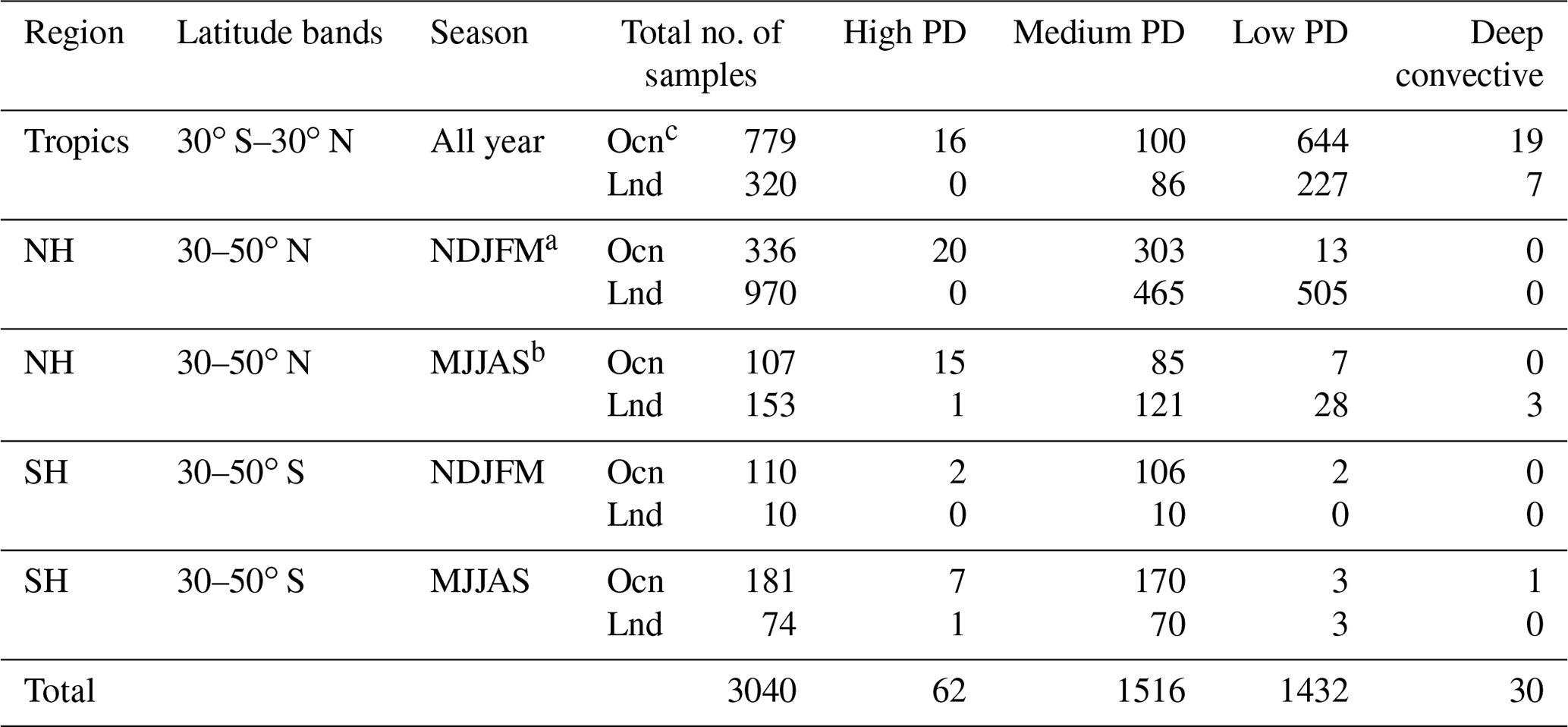
a November–March. b May–September. c “Ocean” includes ocean and coastal footprints, determined by GMI surface flag.
Imperfect matching due to differences in footprint size, view angle (i.e., atmospheric volume along line of sight is different even when the sight lines intersect) time or other factors can distort the compiled statistics. In our case, footprint size and line-of-sight mismatch are likely the largest sources of bias/uncertainty due to imperfect match. On the one hand, the CPR footprint is much smaller than the DPR's and GMI's footprints, and therefore, any cloud–precipitation inhomogeneity on a scale smaller than ∼ 5 km can result in discrepancies that are hard to evaluate. On the other hand, since match-up is defined to happen whenever the CPR beam intercepts with the DPR beam at any altitude and at any DPR view angle, the line-of-sight volume is quite different when DPR is at an off-nadir view angle, and this problem is even more severe for GMI which always views at a slant angle. Even though a cosine function is multiplied to slightly mitigate this issue (Turk, 2017), 3D cloud inhomogeneity and beam-filling effects are again the culprit of uncertainty that is hard to justify. These two problems, however, are expected to be not too serious for our current study, because cloud inhomogeneity inside anvil and stratiform clouds is not as large as in deep convective scenes (Kirstetter et al., 2014). Nevertheless, we know they will increase the uncertainty of our results, and the temporal difference (allowable to be up to 15 min) has a similar impact. Only footprint mismatch might add an extra bias though, as will be discussed in Sect. 3.1.
As this coincident dataset does not contain collocated wind and bright-band information from DPR, collocated indices are matched back to CloudSat ECMWF-AUX and 2A.GPM.DPR data files to extract the wind and bright-band height and width information.
2.4 Radiative transfer model simulations
To help identify the microphysical property distinctions from the observed radar reflectivities and their differences, one radiative transfer model (RTM) and another theoretical calculation are employed. The first RTM and the simulation set-up are described in detail in Leinonen and Szyrmer (2015). An aggregation model (Leinonen, 2013) was used to generate volumetric 3D dry and heavily rimed dendrite aggregates because of their common occurrence in the atmosphere and aggregate efficiently. The particle size distribution (PSD) follows an inverse exponential distribution. The scattering computations for equivalent spheroidal snowflakes were performed using the T-matrix method (TM) based on Mishchenko and Travis (1998) and self-similar Rayleigh–Gan theory (SSRG) method based on Hogan and Westbrook (2014). Using these two computational methods, the dynamic range of the triple-frequency diagram, which will be discussed in Sect. 4, can be largely covered based on many ground observations (e.g., Kneifel et al., 2015, 2016; Kulie et al., 2014; Dias Neto et al., 2019).
The second radiative transfer theoretical calculation is employed to study the density impact on the radar signal difference, which can help us diagnose which types of hydrometers likely dominate the signals under different scenarios. This model is described in detail in Liao and Meneghini (2011). In particular, the snow follows the Gunn–Marshall size distribution (Gunn and Marshall, 1958), and rain follows the Marshall–Palmer size distribution (Marshall and Palmer, 1948). Density and effective diameter follow a power-law form. All particles are assumed to be spheres. Simulations were verified before against airborne campaign data.
3.1 Radar reflectivity differences between high-PD and low-PD scenes
Using 3.5 years of collocated radar reflectivity profiles, we can composite the two-dimensional probability density function (2D PDF) respectively from CloudSat (color shaded) and KuPR (color contours) for the four regimes for the tropics, which is shown in Fig. 2. CloudSat's 2D PDF separates the deep convective scenario clearly from the other three scenarios by having no bright-band kink at ∼ 5 km, a great amount of high clouds and the center of highest occurrence of reflectivity located in the middle-upper troposphere (7–12 km) at around 15 dBZ. The PDF of the low-PD scenario is the closest to that of the deep convective scenario among the remaining three. As PD becomes larger, the bright-band kink at ∼ 5 km becomes more and more distinguished while the maximum occurrence of reflectivity also shifts down toward the middle troposphere (5–8 km). This indicates the scene is more and more stratiform precipitation-like when PD magnitude increases. For KuPR's 2D PDF, as the Ku-band is only sensitive to the precipitation-sized particles, we basically observe the same story as with CloudSat's 2D PDF, except KuPR cannot see high-altitude anvil clouds. Because the KuPR reflectivity is barely sensitive to cloud ice-sized particles, we can also infer large ice particles high in the atmosphere in the deep convective and low-PD cases, while the strong increase in reflectivity towards the bright band in the high-PD case is indicative of aggregates.
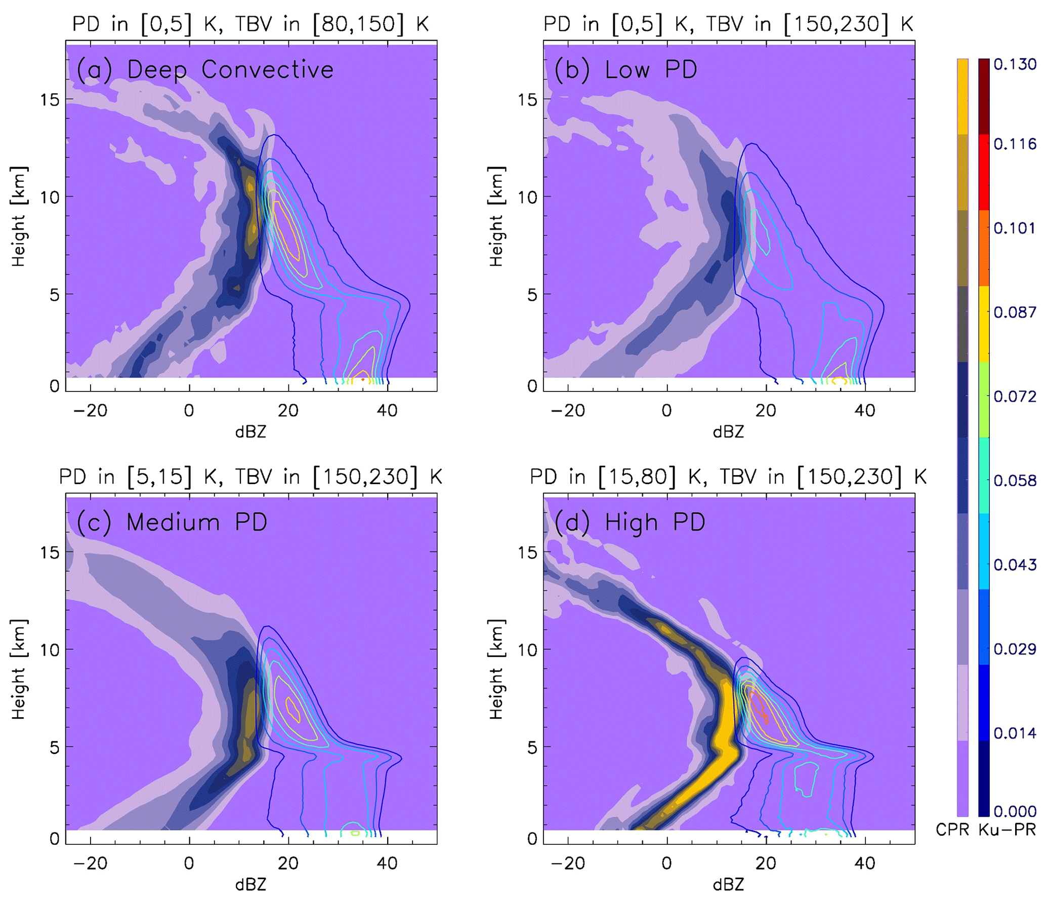
Figure 2The 2D PDFs from CloudSat (color shaded) and DPR Ku (color contours) for the four regimes in Fig. 1 integrated from all tropical (30∘ S–30∘ N) collocated scenes. Panels (a)–(d) correspond to regimes 1–4, respectively. The contour scale is linear and relative to its maximum value.
The 1D plots of mean reflectivity profile from CloudSat, KaPR and KuPR ingeminate the preceding story in a more clear and concise way, as shown in Fig. 3. Basically, Fig. 3 is the weighted mean along the x axis of Fig. 2. Since the 2A.GPM.DPR dataset also reports the altitude of the bright band (i.e., melting layer), Fig. 3b and c are plotted against altitude with respect to the melting level. As we stated in Sect. 2, we do not intend to discuss any signals below the melting layer since CloudSat reflectivity is likely strongly attenuated below the melting layer (Kollias and Albrecht, 2005), and measured reflectivity is used for all three radars without any attenuation or multiple-scattering correction. Above the melting layer, high-level cloud (> 9 km) is thinner while middle-level cloud is thicker (5–8 km) when the cloud regime switches from regime 1 deep convective (dark blue) to regime 4 high-PD (red). If we check the KaPR and KuPR profiles in Fig. 3b and c, however, we see roughly two distinct modes: one includes scenarios 1 and 2 (deep convective and low-PD) that have more precipitation-sized particles throughout the upper-middle troposphere, which might imply that the convection and related cloud are still actively present within the column. On the contrary, the other mode, including scenarios 3 and 4 (medium and high PDs), consist of fewer precipitation-sized particles aloft until close to the top of the melting layer due to increased temperature, where the sharp enhancement of reflectivity indicates fast and efficient growth from small ice particles to large fluffy snow aggregates. This is likely to happen microphysically because the sticking efficiency of two-ice-crystal collision increases rapidly near the melting layer. The latter mode might indicate the late stage of a convection life cycle, where the convective cell disappears and a stable stratiform layer forms to dominate the whole column.

Figure 3The collapsed 1D view of Fig. 2 after weighted averaging along the axis of absolute reflectivity (i.e., x axis) for (a) CloudSat, (b) DPR Ka and (c) DPR Ku. Note that the vertical axis for (a) is absolute altitude, whereas (b) and (c) are altitude with respect to melting level. The red (light blue) line is for the high-PD (low-PD) regime.
Based on Figs. 2 and 3, we can summarize the discrepancies between high- and low-PD scenarios based on pure single-frequency radar observations: the low-PD scenario has more high cloud and large ice particles high into the troposphere, implying active convective updrafts still in the development stage, while the high-PD scenario has much less high cloud but more middle-level cloud, with snow aggregation evident near the top of the melting layer. Therefore, the high-PD scenario shows a distinct bright band, or melting layer signature, which is more stratiform-like and common in the decaying stage of convection. However, these composites are just snapshots, and without actually tracking the entire life cycle of convective system(s), these arguments need further validation. We will show some supportive evidence in Sect. 5 using an ensemble of squall lines. Furthermore, at this point, we cannot yet determine whether the preferably horizontally oriented large snow aggregates above the melting layer cause the high-PD signals or whether the randomly oriented ice–snow particles in the upper-middle troposphere effectively dampen the PD signal in the low-PD scenario from just looking at single-snapshot radar composites. We will discuss each of these possibilities in conjunction with radiative transfer model simulations in Sect. 4.
3.2 Background atmosphere differences between high-PD and low-PD scenes
In this subsection, collocation cases from the tropics, mid-latitude winter and summer are averaged separately considering they represent different weather regimes. Because CloudSat CPR is only operated in daytime mode since 2011, collocation samples over the Southern Hemisphere (SH) are very sparse (Table 1), and therefore only Northern Hemisphere (NH) winter and summer situations are shown in Fig. 4 for temperature and water vapor and Fig. 5 for zonal and meridional winds. The definitions of extended winter (November–March) and summer (May–September) are used in order to enlarge the sample sizes. Although ECMWF-AUX, extracted from ECMWF high-resolution analysis, cannot be considered an “observation”, it is demonstrated to have high quality in capturing the mesoscale to large-scale variations in atmospheric fields (Burgess et al., 2013; Gong et al., 2015). Nevertheless, due to imperfect collocation as we discussed in Sect. 2.3 and the fact that convection is not perfectly represented by forecast models, we would expect the ECMWF-AUX data represent both the ambient and in-cloud dynamic and thermodynamic conditions, which are unfortunately inseparable.
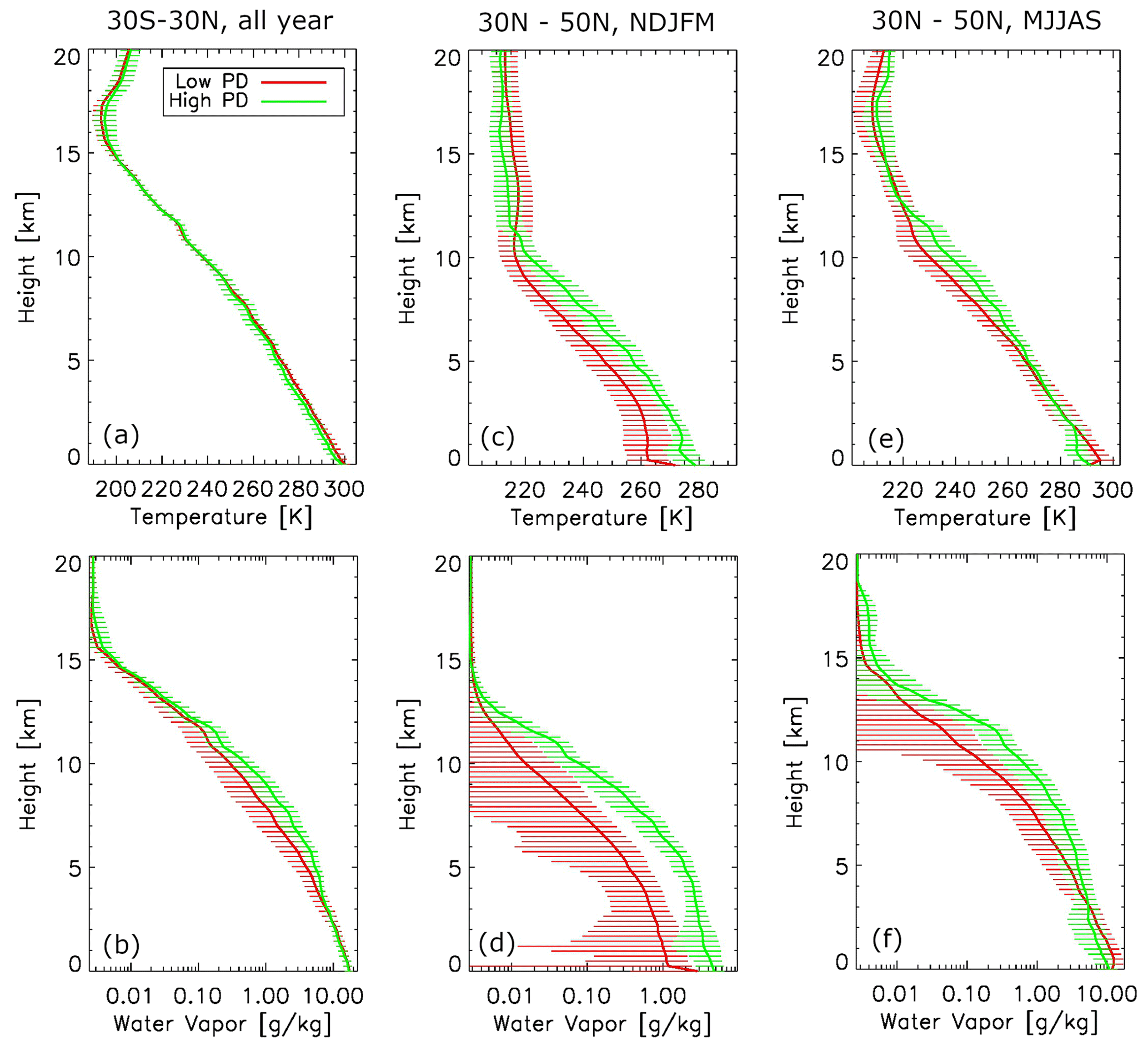
Figure 4Temperature (a, c, e) and water vapor (b, d, f) profiles for high-PD (green) and low-PD (red) scenarios, respectively, for the tropics (a, b, 30 S–30∘ N) averaged over years, Northern Hemisphere extended winter (c, d, 30–50∘ N, November–March) and Northern Hemisphere extended summer (e, f, May–September). Error bars are also included in the same color for every other level.
High- and low-PD regimes do not clearly differentiate from each other on the background temperature profiles as shown in Fig. 4 except for boreal winter when high-PD scenes are on average ∼ 10 K warmer than the low-PD scenes throughout the troposphere. Water vapor amount, however, is consistently higher for high-PD scenes than for low-PD scenes in both tropics and midlatitudes, which translates into higher relative humidity when temperature profiles are almost identical. In the tropics and boreal summer, widespread anvil clouds and stratiform precipitation are mostly tied to deep convective systems such as mesoscale convective systems (MCSs), hurricanes, squall lines, etc. Based on the consistent water vapor discrepancy between the two regimes, we can assert that higher humidity creates a more favorable environmental condition to promote a higher 166 GHz PD signal. Inside clouds, this feature can be understood as follows: higher humidity usually boosts up the deposition growth of ice particles in non-convective regimes. Given the same orientation distribution, larger-sized particles will result in stronger 166 GHz PD, as shown in recent simulations by Brath et al. (2020). Considering this difference in an ambient environment, higher humidity also tends to spawn more vigorous convective systems and/or more organized convection, both of which produce vast areas of stratiform precipitation and therefore a higher 166 GHz signal.

The wind and wind shear differences between the two scenarios are less conclusive. Both of them are not statistically significantly differentiated from one another except for the meridional wind in boreal winter (Fig. 5c, d). But we can see a general pattern that both zonal and meridional low-level shears for high-PD scenes are higher than those for the low-PD scenes, which in general promotes organized convection (MCSs) with large stratiform precipitation areas. In the tropics, there is barely any wind shear for low-PD scenes, but a high-PD scene exhibits stronger meridional southerly shear in the lower level and stronger zonal westerly shear in the upper level. This fits into the conceptual model of a mesoscale convective system (MCS) with a rear-heavy deck in that the lower-level rear inflow jet is nearly perpendicular to upper-level front-to-rear flow (Markowski and Richardson, 2010). Weak shear in low-PD scenes, on the contrary, may indicate that the associated convection is either isolated, mature or dissipated, so stratiform deck area is either very small or not present. For boreal summer (Fig. 5e, f), the stronger lower-level wind shear in high-PD scenes likely promotes more organized convective systems or organized convective vortices, as have been shown in many modeling and observational studies (e.g., Houze, 2004; Chen et al., 2015), so high-PD scenes are likelier to occur if they are caused by large horizontally aligned snow aggregates that are often observed in the stratiform precipitation region. We will show in Sect. 5 that this hypothesis is valid for the quasi-linear MCS and squall line situation.
In boreal winter, convection and stratiform precipitation are most frequently associated with frontal systems. The significant differences in temperature (∼ 10 K), humidity (much wetter for high-PD scenes) and wind (northwest wind for high-PD scenes versus southwest wind for low-PD scenes) all strongly indicate that the two scenarios correspond to two very different weather regimes. The high-PD environment fits the warm front region while low-PD environment fits the cold front and post-frontal sectors. We will not look further into this speculation however, due to the page limit, and will leave this as part of future work.
Our analysis in Sect. 3 supports that the high-PD scenario is tied to a quick growth of ice particles into horizontally aligned snow particles in the middle troposphere above the melting layer. This growth process can be aggregation or water vapor–liquid deposition. However, for the low-PD scenario, we cannot differentiate from single radar reflectivity profiles whether the high-altitude randomly oriented large snow particles effectively damp the PD signal or whether the clouds are dominated by small cloud ice particles to which 166 GHz PD is insensitive even if the particles are preferably horizontally oriented, or some other possibilities. Therefore, in this section, we will try to delineate some of the unique microphysical characteristics that are present in the low-PD scenario and discuss why they lead to the small PD signals at 166 GHz. This investigation will not only help us understand our particular problem more deeply but also help explore the potential usability of PD when active radar is not present, which is most often the case.
As briefly introduced in Sect. 1, triple-frequency radar reflectivity differences can reveal many quantitative structures of ice microphysical properties. In particular, Mason et al. (2019) have demonstrated that PSD shape parameter and ice morphology are the leading two factors that contribute to the spread of reflectivity differences on the triple-frequency diagram, while density and axial ratio play a secondary role. However, unlike the RTM calculation and ground triple-frequency radar measurements that have dedicated perfect-match design, our imperfect matches between CPR and DPR due to temporal, footprint size and viewing geometry differences will confine our analysis here only to a qualitative level. But since DPR Ku and Ka are matched, direct comparison against RTM simulations is possible, as will be shown in Fig. 7 and related discussion.
The dual-frequency ratio (DFR) or dual-wavelength ratio (DWR) between a pair of radar measurements is defined as the reflectivity difference when they are in decibels relative to Z, for example, DFR (dBZ). Two-dimensional PDFs of DFR from high-PD (blue contours) and low-PD (colored shades) scenarios using all collocated samples between 5.5 and 15 km in altitude are presented on the DFR diagram in Fig. 6. Measurements below 5.5 km are excluded to avoid impacts from melting layer and potential saturation below. Because multiple radar profiles are averaged to a single GMI footprint, sensitivity thresholds are changed accordingly (Toyoshima et al., 2015). The thresholds of Yin et al. (2017) are used here to exclude any reflectivity signals below 13, 11 and 2 dB for DPR Ku, DPR Ka and CPR, respectively. DFRs for two ice particle shapes (dendrite aggregate and graupel spheroid) and two riming amounts (unrimed and heavily rimed with effective liquid water path of 2 kg/m2) are calculated and overlaid on Fig. 6b as rough references of theoretical calculated value, which are arbitrarily moved to the right by 5 dBZ in order to match the center of the observed PDFs. See Leinonen and Szyrmer (2015) for details of the RTM, scattering properties and ice morphology definitions.
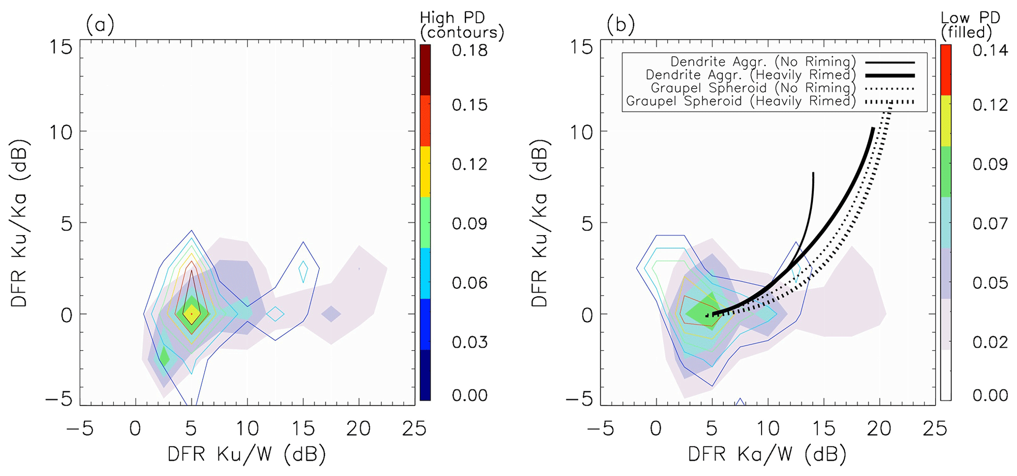
Figure 6The 2D distribution of triple-frequency DFR diagram from the high-PD (dark rainbow-colored outlines) and low-PD (lighter colored shading) regimes composited from all collocated CloudSat and DPR observations: (a) DFRKu∕W versus DFRKu∕Ka; (b) DFRKa∕W versus DFRKu∕Ka. The reflectivity observations are taken from the altitude range of 5.5–15 km to minimize impacts from the melting layer or rain. Model-simulated dendrite (solid) and graupel spheroid (dotted) behaviors are overlaid on (b) for unrimed (thin) and heavily rimed (thick) cases. See Leoinonen and Szyrmer (2015) for model and ice morphology details.
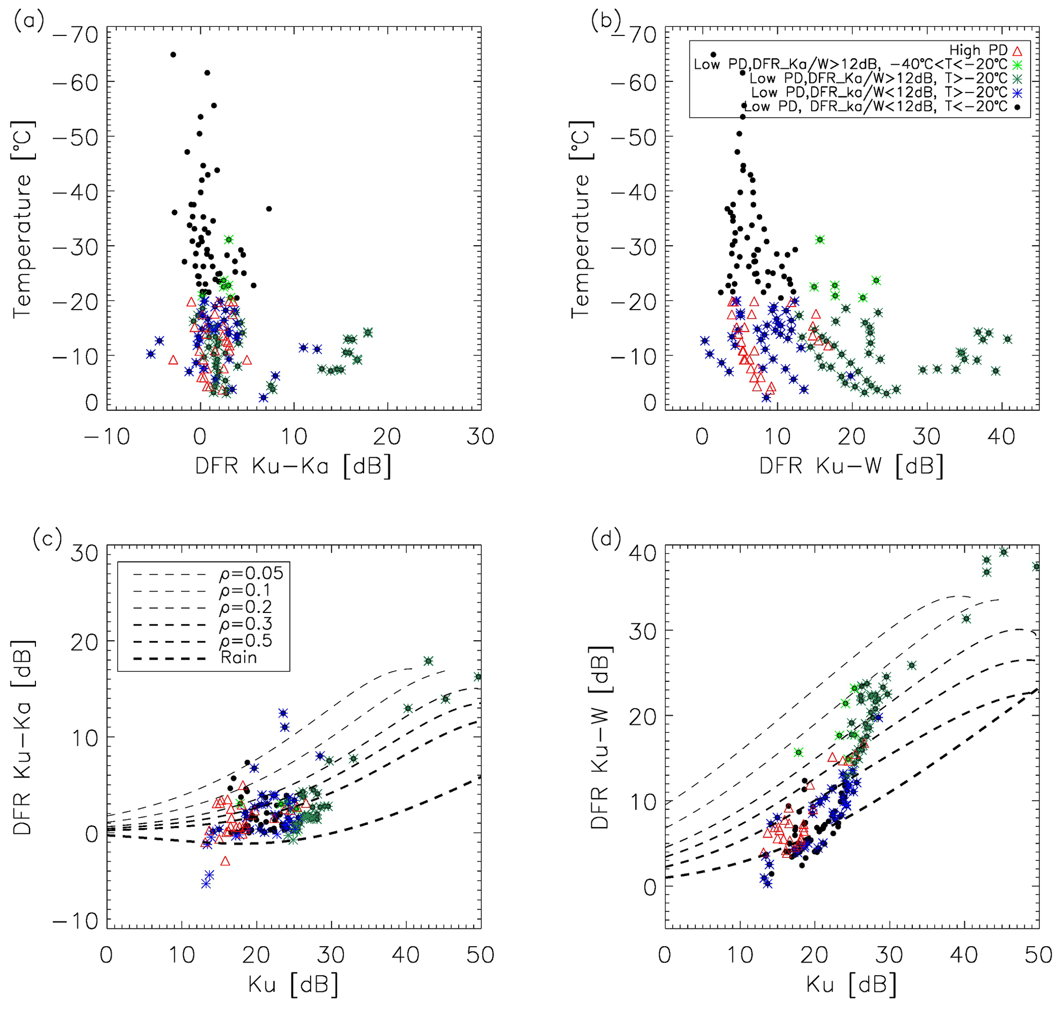
Figure 7Scatter plots of the DFR relationship to temperature (a, b) and to reflectivity (c, d) for high-PD observations (red triangle), low PD with cold temperature and small DFRKu∕Ka (black dots), low PD with warm temperature and small DFRKu∕Ka (blue asterisks), low PD with cold temperature and large DFRKu∕Ka (green asterisks), and low PD with warm temperature and large DFRKu∕Ka (green-blue asterisks). Theoretical calculation of density isolines are overlaid in (c, d) to facilitate our understanding of the density (and habit) of each group of ice particles.
DFRKu∕Ka does not show a significant difference between the two scenarios, but we can see a hint of slight tendency toward larger DFRKu∕Ka values for the high-PD scenario, which suggests that bigger fluffy snow aggregates are the cause of greater Ku and Ka differences. As for DFRKu∕W (Fig. 6a) and DFRKa∕W (Fig. 6b), the largest power does not center around 0 dB but at 5 dB instead, which is likely due to the different minimum detectable reflectivity for CPR and DPR (Skonfronick-Jackson et al., 2019). This is also observed by Yin et al. (2017) for deep convective and stratiform precipitation scenes using collocated CPR–DPR measurements. Other than the biggest enhancement of power centered at 5 dB, which basically suggests that there is little difference in Ku–W and Ka–W response for most of the low-PD samples considering the disparity in their detection thresholds, there are some samples that have very large DFRKu∕W and DFRKa∕W values. These samples line up more closely with the theoretical calculation for heavily rimed graupel, indicating that riming might be the cause for the low-PD signal for these samples. The two modes roughly separate at ∼ 12 dB. This “double-mode” feature in DFRKu∕W and DFRKa∕W strongly suggests that low-PD scenarios have at least two major microphysical contributors.
To further investigate the cause of the double-mode feature in DFRKu∕W and DFRKa∕W, collocated temperature soundings at the same height level of radar reflectivity measurements are used to sort the DFRKu∕Ka (Fig. 7a) and DFRKu∕W (Fig. 7b) into four subcategories for the low-PD scenario: (1) large DFRKa∕W (> 12 dB), cold temperature (); (2) large DFRKa∕W (> 12 dB), warm temperature (); (3) small DFRKa∕W (<12 dB), cold temperature (); and (4) small DFRKa∕W (<12 dB), warm temperature (). The temperature threshold () roughly separates ice particles that are likely unrimed and may be partially rimed. Dias Neto et al. (2019) also found ice PSD widens toward larger DFR in the range, indicating that is a good threshold to use. The high-PD samples are shown as red triangles in Fig. 7. For easy reading, these four subcategories are named “PDLow-DFRLarge-TCold” (light green asterisk), “PDLow-DFRLarge-TWarm” (dark green asterisk), “PDLow-DFRSmall-TCold” (black dot) and “PDLow-DFRSmall-TWarm” (blue asterisk), respectively.
Based on Fig. 7a and b, we can first conclude that all high-PD scenes (red asterisk) are within the relatively warm temperature range (), which is located in the middle-low troposphere in terms of height coordinate (not shown) and hence likely consist of aggregated snow particles rather than ice cloud particles. About 50 % of the low-PD measurements are located in the low-temperature, low-DFR regime (black dots). These are very likely ice cloud particles that are small and hence introduce very weak DFRKu∕Ka and only marginally detectible by CPR considering averaging of multiple CPR profiles onto the GMI footprint significantly degrades the lower boundary of its sensitivity threshold. The rest of the low-PD observations (blue, light green and dark green asterisks) are inherently indistinguishable from high-PD ones on the DFRKu∕Ka axis (Fig. 7a), which indicates they are about the same size as those snow particles that generate the high-PD signal. However, scenes with larger DFRKa∕W values (green asterisk) show a significantly larger DFRKu∕W signal too, as shown in Fig. 7b. Comparison between Fig. 7a and b suggests that there must be certain mechanism(s) for these large-DFRKu∕W (or DFRKa∕W) scenes that effectively decrease the W-band radar reflectivity. These mechanisms could be particle riming, as suggested by the RTM calculations in Fig. 6b, supercooled liquid water that works effectively as a W-band reflectivity damper as well as 166 GHz PD damper (Xie et al., 2018), or water vapor that also impacts the W-band much more seriously than Ku- or Ka-bands. According to Fig. 4, high-PD scenes unanimously have higher water vapor amounts than low-PD scenes. Therefore, water vapor abundance could serve as a plausible explanation to explain the small DFRKu∕W for high-PD scenes (red asterisks in Fig. 7) but not for low-PD scenes. Therefore, frozen particle riming and supercooled liquid water are the two most plausible candidates to explain the behaviors of those green asterisks (PDLow–DFRLarge). For PDLow–DFRSmall scenes (black dot and blue asterisks), we have discussed that black dot scenes probably correspond to cloud ice particles because of cold temperature and relatively high altitude where they are located, and the blue asterisk scenes may be explained as randomly oriented unrimed snow aggregates.
Particle density isolines overlaid on DFR-Z plots (Z denotes “plots”) can help further delineate the different microphysical regimes that high-PD and low-PD scenarios fall into, as shown in Fig. 7c and d. These isolines are replicated from the same scattering model and setups of Liao and Meneghini (2011). Keep in mind that Fig. 7c is comparable quantitatively to the theoretical isolines (other than the water vapor not being corrected) as Ku-Ka are perfectly matched in beam, while Fig. 7d can only assist our interpretation qualitatively. The high-PD scenes are separated from the three low-PD subcategories in Fig. 7c and more clearly in Fig. 7d (PDLow-DFRSmall-Tcold samples; the black dots in Fig. 7a and 7b are not shown because they are likely from cloud ice particles). In particular, one can see that given the same small DFR, the blue asterisks are generally denser than red triangles. This agrees with our earlier hypothesis that the high PD is mainly induced by fluffy snow aggregates where ice crystals are loosely attached to each other during the rapid aggregation process and therefore tend to fall slowly and orient horizontally because of the large geometric area. On the other hand, some of the low-PD signals (blue asterisks) are induced by denser snow aggregates that are comparable in effective diameter with those ones in the high-PD scenes. However, because the ice crystals are more tightly collided together in these snow aggregates, they tend to not have a preferred shape or orientation. The dark green asterisks are suggested by Fig. 7c to be even denser (except a few outliers on the top right corner), which strongly suggests that they are possibly experiencing riming. Figure 7d tells a contradictory story about these green asterisks, however. But noting that observations in Fig. 7d are not directly comparable with RTM calculations because of imperfect volume matching, we focus on and trust more the results presented in Fig. 7c (and similar Fig. 7a).
To summarize this section, we are able to provide more evidence that the high-PD signal is mainly induced by horizontally oriented fluffy snow aggregates while also successfully delineating several possible microphysical mechanisms of low-PD signals, which are (1) small cloud ice particles, (2) more densely aggregated snow particles that tend to orient randomly, (3) riming snow and (4) supercooled liquid water. This section demonstrates the value and importance of closely matched triple-frequency radar measurements in conjunction with accurate atmospheric soundings. We also find that 166 GHz PD indeed is primarily sensitive to the orientation of large snow particles instead of small cloud ice particles. Adding polarization measurements at a sub-millimeter frequency (e.g., 640 GHz from the Ice Cloud Imager sensor) may likely aid in disentangling orientation of cloud ice from that of snow particles from a passive sensor.
Convective systems usually experience a complete life cycle of development. During the developing stage, the deep convective tower(s) quickly shoots up and anvil deck quickly spreads out. During the decaying stage, the convective core dissipates and is replaced with a stable stratiform precipitating area. By far it is established that the leading anvil cloud is likely associated with low PD, while high PD is likely associated with a trailing stratiform layer. Can we then use PD as a proxy to tell which stage a convective system is at? If yes, does high PD necessarily imply more intense surface precipitation compared to a low-PD regime given the same TB range? In this section, we will explore the potential usefulness of PD on a relatively simple natural test bed – squall line system. Squall lines, as a subset of typical convective systems, are an ideal test bed because they are quasi-linear (i.e., no rotation like hurricanes or frontal systems), and the anvil head in the leading edge and the vast area of stratiform precipitation layer in the trailing edge are easily separable on GMI images.
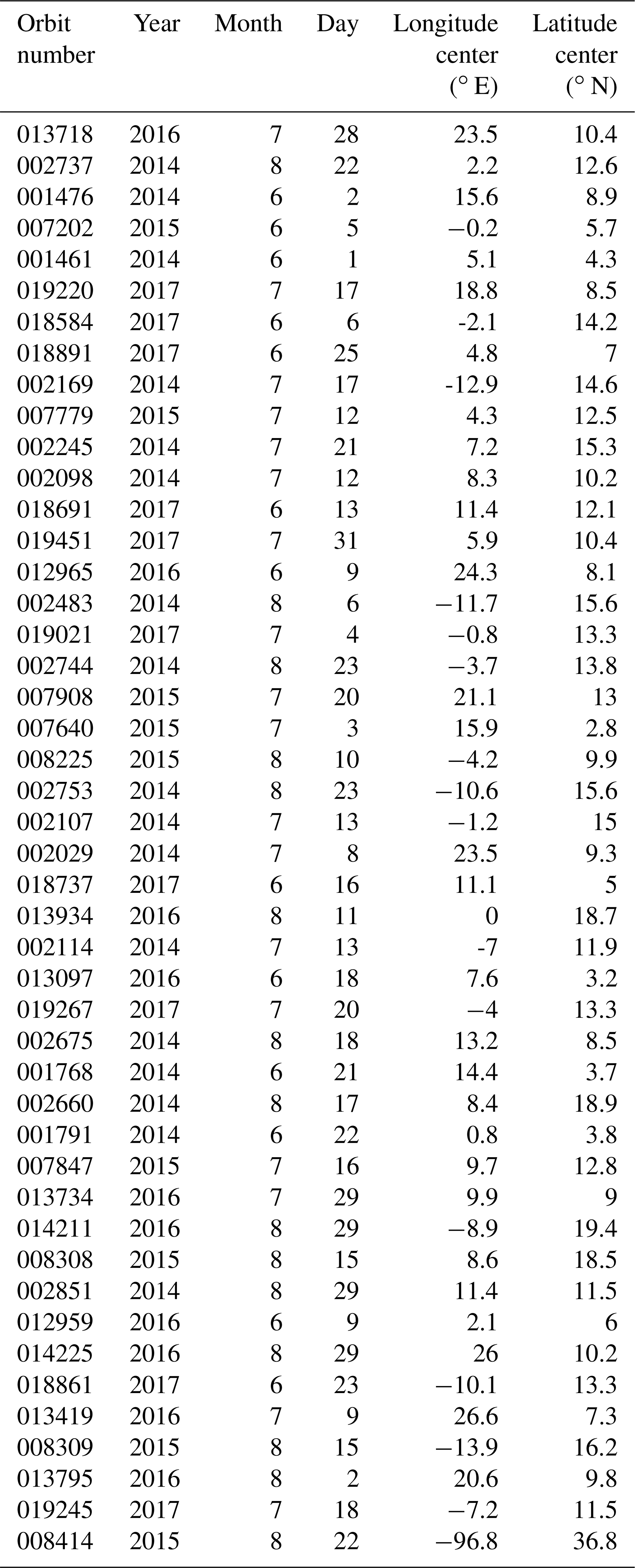
We manually selected 47 squall line cases from GPM observations (see Table A1 for detailed location, orbit number and date). For these 47 cases, we require the following: (1) the line of deep convection must be captured by DPR and (2) the squall line moving direction must be quasi-perpendicular to GPM orbit. The latter requirement assures that each GMI conical scan can slice through the squall line whenever the collocated DPR captures a deep convective core. An example of a selected case is given in Fig. 8, where the leading edge and trailing edge are to the left and right, respectively, because this case happened over the Sahel. From Fig. 8b we can clearly visualize that PD is significantly higher behind the line of deep convection identified from Fig. 8c on the DPR image. To composite the ensemble of 47 cases together, we first identify the footprint location on each DPR scan that has the maximum KuPR-retrieved near-surface precipitation rate (PRsfc), which is required to be beyond a threshold (PRsfc>25 mm/h). This threshold is arbitrarily set but works robustly against a range of values (20–50 mm/h are tested, and only the number of qualified samples is changed without altering the conclusion). The location of identified deep convective centers is shown in Fig. A1 in the Appendix. Once the center of convection on a DPR scan is identified, the collocated GMI footprint and its index on the scan are then pinpointed. Next, the footprints corresponding to the leading edge and trailing edge are sorted accordingly against the convective center. Lastly, all selected GMI and DPR scans are aligned together with GMI's deep convective center footprint in the middle, trailing edge to the left and leading edge to the right. The averaged cross sections of 166 GHz TB and PD responses for each case are shown as black lines in Fig. 9a and b, respectively, while the ensemble means are the red bold lines. The DPR scan widths are shown as light grey rectangles in Fig. 9a and b for comparison.
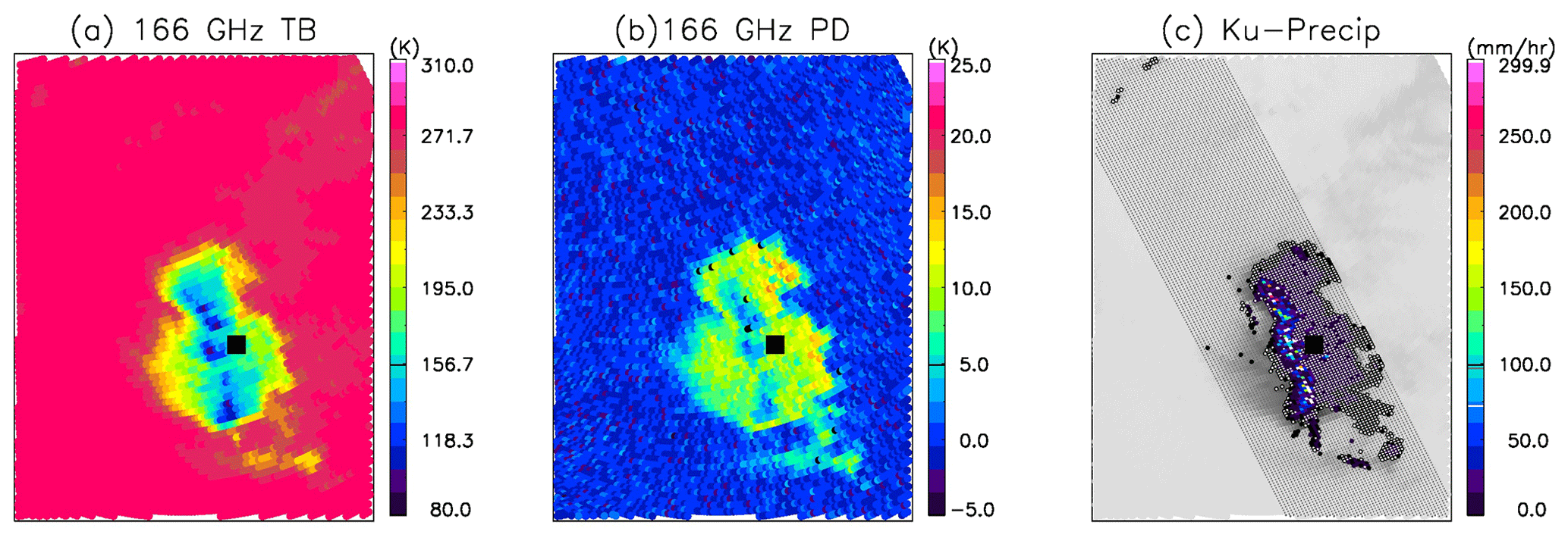
Figure 8A squall line case captured by GMI and DPR exhibits larger PD behind (to the right) the deep convective front than in the leading edge (to the left). (a) The 166 GHz TB, (b) 166 GHz PD and (c) KuPR retrieved surface precipitation rate (color) on DPR swath (grey) overlaid on top of GMI 166 GHz PD (light grey), where convective pixels are colored and stratiform pixels are stippled with white circles. The black rectangle is a reference point for easy inter-panel comparison. This squall line case occurred on 20 July 2015 (orbit no. 007908) over Chad, Africa.
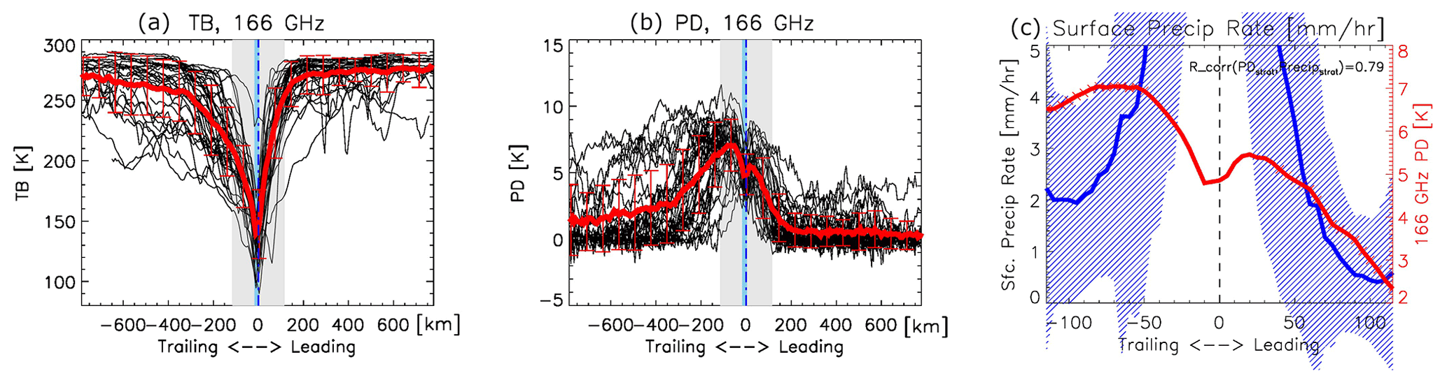
Figure 9The 166 GHz TB (a) and PD (b) distribution across the squall line center (0 at horizontal axis) for all 47 squall line cases (black) and their mean (thick red) and standard deviation (thin red error bars). The trailing edge is to the left and the leading edge is to the right. The squall line case details can be found in Table A1 in the Appendix. Light grey rectangles in (a) and (b) correspond to KuPR coverage. In (c), mean surface precipitation rate (PRsfc) retrieved from KuPR is displayed as the thick blue line across the squall line center with standard deviation shown in blue hatched areas. The 166 GHz PD in the grey area in (b) is overlaid as the thick red line in (c). Deep convective rainy footprints (PRsfc>5 mm/h) are excluded for plotting because our PD hypothesis only works at the stratiform region. The Pearson rank correlation between PRsfc and PD is 0.79 (significance at 99.9 % confidence level) after excluding the deep convective footprints.
Both TB and PD across the squall line are asymmetric about the deep convective center. The ensemble mean of TB is ∼ 10 K colder to the trailing edge than to the leading edge, which translates into a radiatively thicker anvil cloud/falling snow layer behind the squall line than ahead of it. The width of depression of TB is also much broader in the trailing edge than in the leading edge. Both features agree well with our conceptual picture of the squall line system (Houze, 2004). Cetrone and Houze (2011) selected and studied another ensemble of Africa squall lines, and they found that the geometric thicknesses of leading anvil and trailing stratiform cloud layers are not significantly different. So a radiative thickness difference of ∼ 10 K in our ensemble case could indicate larger snow particles in the trailing edge than fresh anvil cloud ice particles in the leading edge.
The ensemble mean of PD, as expected, displays a double-peak in front and behind the deep convective center. The peak occurs ∼ 70 and ∼ 25 km away from the center on the trailing edge and leading edge, respectively. The magnitude of PD in the trailing edge is apparently larger (7 K) and spread more wildly than that in the leading edge (5.5 K). Interestingly, PD in the deep convection is not zero but ∼ 4.5 K. One can see from the general statistics in Fig. 1 that PD is ∼ 4 K when TB is about 120 K, which is consistent with the mean TB and PD values we found for deep convective cores from our squall line ensemble. We can further see from Fig. 10b when the distribution of PD is plotted that a discernable number of convective pixels have large PD values and hence skewed the mean toward the positive side. A 5.5 K peak PD value in the leading edge suggests that there is also a significant number of large horizontally aligned ice particles inside the leading anvil decks, which is consistent with previous findings in Cetrone and Houze (2011).
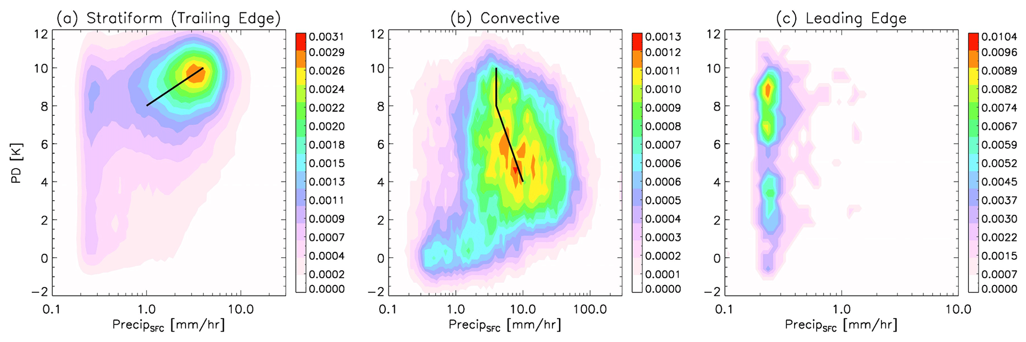
Figure 10Joint surface precipitation and 166 GHz PD distribution function (2D PDF) in the (a) stratiform, (b) convective and (c) leading edge of the squall lines. DPR stratiform, convective and other flags are employed to differentiate different precipitation types.
The PRsfc–PD relationship is further evaluated. We perform this evaluation from two perspectives. First, we would like to check whether across the squall line precipitation intensity is significantly different or not and whether it is related to the magnitude of PD. A threshold of 5 mm/h is used as a rough threshold to exclude convective rain scenes because the magnitude of PD inside convection involves too many complicated dynamic and microphysical processes and this is not what this paper is aiming for. Away from the convection, a correlation of 0.79 (significant at 99.9 % confidence level) is achieved, as shown in Fig. 9c. PRsfc reaches 2 mm/h in the stratiform zone behind the deep convection, which is <1 mm/h in the leading edge. Considering that it takes some time for snow aggregates to fall down to the surface while the squall line keeps on moving forward, a spatially lagged correlation would be more physically meaningful (Gong et al., 2017). Unfortunately, the DPR scan is too narrow for us to conduct such a lag-correlation test. The other way to evaluate the PRsfc–PD relationship is to composite the statistics. Since Level 2 DPR retrievals provide the precipitation type flag, which classifies precipitation into three types, stratiform, convective and other, we use these three flags to separate our ensemble data into three categories and composite the 2D PDF of PRsfc–PD for each of them. Note that “stratiform precipitation” flag only occurs in the trailing edge, but the “other precipitation” flag may include precipitation happening everywhere within the domain, so we add an extra criterion that only the footprints located at the leading edge are selected to use. The 2D PDF composites of PRsfc–PD for the stratiform, deep convective and leading edge are shown in Fig. 10, which are completely different, confirming that the cloud–precipitation process belongs to completely different regimes for each of the three types. The maximum likelihood of PD in the stratiform region reaches ∼ 10 K, while in the convective regime it centers around 4–6 K, and the value spreads out in the leading edge from as small as 2 K to up to 10 K. PD is only positively correlated with surface precipitation rate in the stratiform region and only when PD is high. A 2 K increase in PD from 8 to 10 K corresponds to a 4-fold increase in PRsfc from 1 to 4 mm/h (note that the horizontal axis in Fig. 10 is logarithmic), which is quite remarkable and again demonstrates the importance of ice microphysics to the local precipitation intensity and its variation. In the convective regime, PD is weakly negatively correlated with surface precipitation, but when PD is large (> 8 K roughly), the correlation becomes negligible or even positive, which is likely due to the fact that these pixels are close to the boundary of convective–stratiform separation. Keep in mind that these correlations (Fig. 10) can only be performed within the narrow DPR swath (grey bars in Fig. 9a and b) where both the DPR-identified precipitation flag and collocated 166 GHz PD measurements are available, while the majority of stratiform precipitation and fresh anvil leading head are outside of the DPR swath using our current ensemble technique. Thus Fig. 10 is just looking at a small part of the entire picture, and more comprehensive works are needed in the future to recover the whole picture.
Although the steep slope means that PRsfc is very sensitive to the magnitude of PD in the stratiform region when PD is large, the overall spread of the 2D PDF suggests that we cannot incautiously use PD as a new parameter for surface precipitation retrieval. Rather, this finding suggests that 166 GHz PD could be and should be considered an extra constraint to GMI-only precipitation retrieval because of its added value in certain regimes, which remains a worthwhile topic for future exploration. Meanwhile, we can clearly see from Fig. 10c that in non-stratiform regimes (i.e., leading edge in our squall line cases), PD is not correlated with PRsfc at all. The contrast of 2D PDF shapes in the trailing edge versus in the leading edge again goes along with our understanding that large horizontally aligned snow aggregates tend to occur in the stratiform layer and tend to precipitate down in a short frame of time, while it takes longer for those relatively small snowflakes hanging up in the fresh anvil deck in the leading edge to fall to the ground, the latter of which will apparently enjoy varied experiences during the falling process. Furthermore, PD from 166 GHz cannot be used solely to diagnose the life stage of a convective system either, but multiple spaciously coherent PD measurements spanning from microwave (MW) to sub-millimeter or even infrared spectra may realize this function eventually without any involvement of active remote sensing. For example, Olson et al. (2001) developed a passive MW-only flag system, called the convective–stratiform index (CSI) to flag out convective and stratiform scenes, which relies on a combination use of TB and TB gradient at 19, 37 and 85 GHz, as well as 85 GHz PD magnitude. This was back in the TRMM era when 85 GHz was the highest available frequency making measurements at both V-pol and H-pol. Although not shown or discussed in the main text, Fig. A2 includes the same squall line ensemble of TB and PD at 89 GHz from GMI measurements. We can see that 89 GHz PD spreads all over the place and does not show a good correspondence to deep convective or stratiform zones (Fig. A2 in the Appendix). Based on our investigation in this paper, 166 GHz PD is likely a better candidate to update the CSI algorithm, which is left for exploration in the future.
At 166 GHz, GMI currently makes the highest frequency of dual-polarized microwave radiance measurements from space. Gong and Wu (2017) and Gong et al. (2017) thoroughly studied the PD and TB signals from GMI, and they laid out several possible microphysical mechanisms that can explain the PD signal under different TB regimes. In this paper, leveraging the collocated DPR and CPR radar reflectivity measurements, we are, for the first time, able to delineate the microphysical properties not only for high-PD scenes but also for low-PD scenes for the same moderately cold TB regime. As high-frequency MW radiance measurements can only be used to infer column-integrated mass quantities such as ice water path for this moderately cold TB regime, the PD measurement allows us to diagnose much more information about the microphysical processes occurring in the profile. The analysis of PD and radar data in this paper suggests that 166 GHz PD is closely associated with horizontally oriented large fluffy snow aggregates in the stratiform precipitation layers that tend to melt and fall as precipitation. Low 166 GHz PD signals, however, are associated with more complicated situations. At least four mechanisms are found to possibly be responsible for the low-PD signals: (1) small cloud ice particles up aloft that 166 GHz PD is barely sensitive to, (2) more densely aggregated snow particles that tend to orient randomly, (3) riming snow particles that effectively damp the PD signal and (4) supercooled liquid water that also damps the PD signal. With only 166 GHz TB and PD observations, it is difficult to distinguish which mechanism dominates a single scene, but better diagnostic approaches can be developed in the future using adjacent passive-only observations in conjunction with accurate atmospheric background measurements or analysis. As sub-millimeter radiances are more sensitive to smaller particles, multifrequency PD measurements at MW and sub-millimeter spectra could be the best approach to separate particle size, shape and orientation information from cloud ice and snow aggregates, as already shown via RTM simulations by Brath et al. (2020).
This paper also demonstrates the value of using collocated triple-frequency radar measurements to disentangle the complicated microphysical characteristics along the passive MW line of sight. However, due to beam-filling and other mismatch issues (e.g., footprint, view angle and temporal disparities), our “pseudo-triple-frequency” radar (DPR + CPR) statistics are distorted and displaced and therefore cannot be directly compared with RTM simulations quantitatively. Since a perfectly matched triple-frequency radar space mission will be likely unavailable in the near future, using collocated ground or “pseudo-collocated” space radar measurements together with passive MW PD observations is probably the best approach to extend our knowledge about passive MW PD signals for a better scientific and/or operational use. Besides DFR, other parameters should also be inspected in future work. For example, the dual-wavelength ratio (DWR) can provide information on ice particle size without being influenced by particle concentration.
We lastly scrutinized 166 GHz PD and DPR behaviors in an ensemble of squall line cases. We found out that PD is larger in the trailing edge where large snow aggregates are predominant in the stratiform layer, while PD is smaller in the leading edge where fresh anvil decks dominate the scene. Surface precipitation, as expected, is positively correlated with PD in the stratiform region when high PD occurs. Three possible ways of using PD are then discussed, which are (1) using 166 GHz PD to constrain passive-only surface precipitation retrieval under certain conditions, (2) using multifrequency PD and TB measurements to help diagnose the life stage of a convective system and (3) improving the design of passive-only stratiform–convective precipitation flags. They will be explored in the future.

Figure A1The geographic distribution of the 47 squall line cases that are selected. Red dots are the location of the identified deep convective center (i.e., maximum PRsfc while PRsfc>25 mm/h threshold) on each KuPR scan. Each scan swath is then aligned against this center location (setting as 0) to make the composites shown in Figs. 9 and A2.
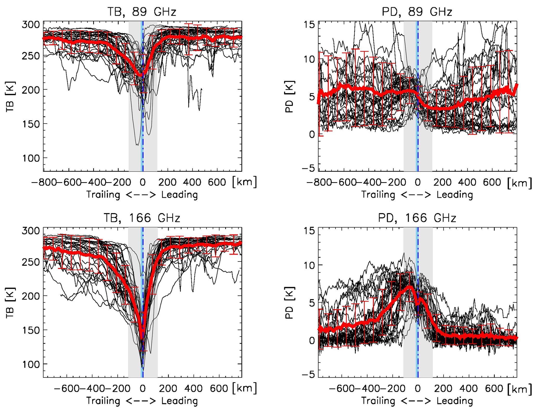
Figure A2The bottom panels are the same as Fig. 9a and b, and the top panels are similar, except they are for 89 GHz. One can see that the 89 GHz PD signal is not as clean as that at 166 GHz since the 89 GHz's PD is also strongly impacted by surface emission and liquid cloud/raindrop emission.
Table A1Details about the 47 squall line cases we selected. The first column lists the GPM orbit number. The second–fourth columns include year, month and day of the event, and the last two columns are the longitude and latitude of the reference center (i.e., black rectangle in Fig. 8 for easy comparison, not necessarily the storm center).
GPM data and collocated GPM CPR data are available to the public at NASA PPS FTP at https://pmm.nasa.gov/data-access/downloads/gpm (NASA, 2017). CloudSat and ECMWF-AUX data are made available from CloudSat FTP at http://www.cloudsat.cira.colostate.edu/order-data (Cronk and Partain, 2017). High- and low-PD statistics can be provided to readers upon request.
JG and SJM initiated the original idea. JG conducted most of the data analysis and result interpretation. SJM provided part of the Ku and Ka CFAD composites and polished the writing. XZ, DLW and XL were heavily involved in interpreting the results. In addition, XL provided the squall line ensemble cases. SK and DO provided the theoretical calculations of the triple-frequency radar DFR and helped explain some of the observational property. LL provided the theoretical calculations of the density isolines. DB provided the global model perspective for this study.
The authors declare that they have no conflict of interest.
We are grateful to the dedicated experts from the CloudSat and GPM teams who maintain and distribute the high scientific-quality Level 1 and Level 2 data. We are particularly in debt to GPM precipitation feature product producer Chuntao Liu at Texas A&M University Corpus Christi. Discussions with Manfred Brath, Ian Adams and Chuntao Liu, among others, greatly helped make this paper better. In addition, we are thankful to the three anonymous reviewers and Toshi Matsui for providing insightful comments that helped greatly in making the presentation clearer. This work was mainly conducted under the support from NASA grant no. 80NSSC20K0087. Funding support from grant no. NNX16AM06G and NASA ROSES NNH18ZDA001N-RRNES is also highly appreciated. Davide Ori and Stefan Kneifel acknowledge funding from the German Research Foundation (DFG) under grant KN 1112/2-1 as part of the Emmy-Noether Group Optimal combination of Polarimetric and Triple Frequency radar techniques for Improving Microphysical process understanding of cold clouds (OPTIMIce).
This work is mainly conducted under the support of NASA (grant nos. 80NSSC20K0087, NNX16AM06G, NNH18ZDA001N-RRNES). Davide Ori and Stefan Kneifel acknowledge funding from the German Research Foundation (DFG) (under grant KN 1112/2-1) as part of the Emmy-Noether Group Optimal combination of Polarimetric and Triple Frequency radar techniques for Improving Microphysical process understanding of cold clouds (OPTIMIce).
This paper was edited by Jianping Huang and reviewed by Toshi Matsui and three anonymous referees.
Brath, M., Ekelund, R., Eriksson, P., Lemke, O., and Buehler, S. A.: Microwave and submillimeter wave scattering of oriented ice particles, Atmos. Meas. Tech., 13, 2309–2333, https://doi.org/10.5194/amt-13-2309-2020, 2020.
Burgess, B. H., Erler, A. R., and Shepherd, T. G.: The troposphere-to-stratosphere transition in kinetic energy spectra and nonlinear spectral fluxes as seen in ECMWF analyses, J. Atmos. Sci., 70, 669–687, https://doi.org/10.1175/JAS-D-12-0129.1, 2013.
Cetrone, J. and Houze, R. A: Leading and Trailing Anvil Clouds of West African Squall Line, J. Atmos. Sci., 68, 1114–1123, https://doi.org/10.1175/2011JAS3580.1, 2011.
Chase, R. J., Finlon, J. A., Borque, P., McFarquhar, G. M., Nesbitt, S. W., Tanelli, S., Sy, O. O., Durden, S. L., and Poellot, M. R.: Evaluation of triple-frequency radar retrieval of snowfall properties using coincident airborne in situ observations during OLYMPEX, Geophys. Res. Lett., 45, 5752–5760, https://doi.org/10.1029/2018GL077997, 2018.
Chen, Q., Fan, J., Hagos, S., Gustafson Jr., W., and Berg, L. K.: Roles of wind shear at different vertical levels: cloud system organization and properties, J. Geophys. Res.-Atmos., 120, 6551–6574, https://doi.org/10.1002/2015JD023253, 2015.
Cronk, H. and Partain, P.: CloudSat ECMWF-AUX Auxillary data product process description and interface control document, last access: http://www.cloudsat.cira.colostate.edu/sites/default/files/products/files/ECMWF-AUX_PDICD.P_R05.rev0_.pdf (last access: 29 October 2020), 2017.
Defer, E., Galligani, V. S., C. Prigent, C., and Jimenez, C.: First observations of polarized scattering over ice clouds at close-to-millimeter wavelengths (157 GHz) with MADRAS on board the Megha-Tropiques mission, J. Geophys. Res.-Atmos., 119, 2014JD022353, https://doi.org/10.1002/2014JD022353, 2014.
Dias Neto, J., Kneifel, S., Ori, D., Trömel, S., Handwerker, J., Bohn, B., Hermes, N., Mühlbauer, K., Lenefer, M., and Simmer, C.: The TRIple-frequency and Polarimetric radar Experiment for improving process observations of winter precipitation, Earth Syst. Sci. Data, 11, 845–863, https://doi.org/10.5194/essd-11-845-2019, 2019.
Field, P. R. and Heymsfield, A. J.: Importance of snow to global precipitation, Res. Lett., 42, 9512–9520, https://doi.org/10.1002/2015GL065497, 2015.
Eriksson, P., Jamali, M., Mendrok, J., and Buehler, S. A.: On the microwave optical properties of randomly oriented ice hydrometeors, Atmos. Meas. Tech., 8, 1913–1933, https://doi.org/10.5194/amt-8-1913-2015, 2015.
Evans, K.F., Wang, J. R., Starr, D. O'C., Heymsfield, G., Li, L., Tian, L., Lawson, R. P., Heymsfield, A. J., and Bansemer, A.: Ice hydrometeor profile retrieval algorithm for high frequency micro-wave radiometers: application to the CoSSIR instrument during TC4, Atmos. Meas. Tech., 5, 2277–2306, https://doi.org/10.5194/amt-5-2277-2012, 2012.
Gong, J. and Wu, D. L.: CloudSat-constrained cloud ice water path and cloud top height retrievals from MHS 157 and 183.3 GHz radiances, Atmos. Meas. Tech., 7, 1873–1890, https://doi.org/10.5194/amt-7-1873-2014, 2014.
Gong, J. and Wu, D. L.: Microphysical Properties of Frozen Particles Inferred from Global Precipitation Measurement (GPM) Microwave Imager (GMI) Polarimetric Measurements, Atmos. Chem. Phys., 17, 2741–2757, https://doi.org/10.5194/acp-17-2741-2017, 2017.
Gong, J., Yue, J., and Wu, D. L.: Global survey of concentric gravity waves in AIRS images and ECMWF analysis, J. Geophys. Res.-Atmos., 120, 2210–2228, https://doi.org/10.1002/2014JD022527, 2015.
Gong, J., Zeng, X., Wu, D. L., and Li, X.: Diurnal Variation of Tropical Ice Cloud Microphysics: Evidence from Global Precipitation Measurement Microwave Imager (GPM-GMI) Polarimetric Measurements, Geophys. Res. Lett., 45, 1185–1193, https://doi.org/10.1002/2017gl075519, 2017.
Gettleman, A., Liu, X., Ghan, S. J., Morrison, H., Park, S., Conley, A. J., Klein, S. A., Boyle, J., Mitchell, D. L., and Li, J.-L. F.: Global simulations of ice nucleation and ice supersaturation with an improved cloud scheme in the Community Atmosphere Model, J. Geophys. Res.-Atmos., 115, D18, https://doi.org/10.1029/2009JD013797, 2010.
Gunn, K. L. S. and Marshall, J. S.: The distribution with size of aggregate snowflakes, J. Meteor., 15, 452–461, https://doi.org/10.1175/1520-0469(1958)015<0452:TDWSOA>2.0.CO;2, 1958.
Hogan, R. J. and Westbrook, C. D.: Equation for the microwave backscatter cross section of aggregate snowflakes using the self-similar rayleigh-gans approximation, J. Atmos. Sci., 9, 3292–3301, https://doi.org/10.1175/JAS-D-13-0347.1, 2014.
Houze Jr., R. A.: Mesoscale Convective Systems, Rev. Geophys., 42, https://doi.org/10.1029/2004RG000150, 2004.
Kirstetter, P.-E., Hong, Y., Gourley, J. J., Schwaller, M., Petersen, W., and Cao, Q.: Impact of sub-pixel rainfall variability on spaceborne precipitation estimation: evaluating the TRMM 2A25 product, Q. J. Roy. Meteor. Soc., 141, 953–966, https://doi.org/10.1002/qj2416, 2014.
Kneifel, S., Kulie, M. S., and Bennartz, R.: A triple-frequency approach to retrieve microphysical snowfall parameters, J. Geophys. Sci., 116, https://doi.org/10.1029/2010JD015430, 2011.
Kneifel, S., Lerber, A. v., Tiira, J., Moisseev, D., Kollias, P., and Leinonen, J.: Observed relations between snowfall microphysics and triple-frequency radar measurements, J. Geophys. Sci., 120, 6034–6055, https://doi.org/10.1002/2015JD023156, 2015.
Kneifel, S., Kollias, P., Battaglia, A., Leinonen, J., Maahn, M., Kalesse, H., and Tridon, F.: First observations of triple-frequency radar Doppler spectra in snowfall: interpretation and applications, Geophys. Res. Lett., 43, 2225–2233, https://doi.org/10.1002/2015GL067618, 2016.
Kollias, P. and Albrecht, B.: Why the melting layer radar reflectivity is not bright at 94 GHz?, Geophys. Res. Lett., 32, https://doi.org/10.1029/2005GL024074, 2005.
Kulie, M. S., Hiley, M. J., and Bennartz, R.: Triple-frequency radar reflectivity signatures of snow: observations and comparisons with theoretical ice particle scattering models, J. Appl. Meteorol. Clim., 53, 1080–1098, https://doi.org/10.1175/JAMC-D-13-066.1, 2014.
Kummerow, C. D., Randel, D. L., Kulie, M., Sang, N.-Y., Ferraro, R., Munchak, S. J., and Petkovic, V.: The evolution of the Goddard profiling algorithm to a fully parametric scheme, J. Atm. Ocn. Tech., 32, 2265–2280, https://doi.org/10.1175/JTECH-D-15-0039.1, 2015.
Leinonen, J.: Impact of the microstructure of precipitation and hydrometeors on multi‐frequency radar observations, PhD thesis, Aalto Univ., Espoo, Finland, 2013.
Leinonen, J. and Szyrmer, W.: Radar signatures of snowflake riming: a modeling study, Earth Space Sci., 2, 346–358, https://doi.org/10.1002/2015EA000102, 2015.
Liao, L. and Meneghini, R.: A study on the feasibility of dual-wavelength radar for identification of hydrometeor phases, J. Appl. Meteorol. Clim., 50, 449–456, https://doi.org/10.1175/2010JAMC2499.1, 2011.
Liou, K. N., Takano, Y., Yang, P., and Gu, Y.: Radiative transfer in cirrus clouds: Light scattering and spectral information, in: Cirrus, edited by: Lynch, D. K., Sassen, K., Liou, K. N., Cosh, M., and Brutsaet, W., Oxford Univ. Press, New York, 265–296, 2002.
Luo, Z., Liu, G. Y., and Stephens, G. L.: CloudSat adding new insight into tropical penetrating convection, Geophys. Res. Lett., 35, https://doi.org/10.1029/2008GL035330, 2008.
Manaster, A., O'Dell, C. W., and Elsaesser, G.: Evaluation of cloud liquid water path trends using a multidecadal record of passive microwave observations, J. Clim., 30, 5871–5884, https://doi.org/10.1175/JCLI-D-16-0399.1, 2017.
Marchand, R. and Mace, G.: Level 2 GEOPROF product process description and interface control document, P1_R05, available at: http://www.cloudsat.cira.colostate.edu/sites/default/files/products/files/2BGEOPROF_PDICD.P1_R05.rev0__0.pdf (last access: 29 October 2020), 2018.
Markowski, P. and Richardson, Y.: Mesoscale meteorology in midlatitudes, chap. 9, mesoscale convective systems, ISBN: 978-0-470-74213-6, https://doi.org/10.1002/9780470682104, 2010.
Marshall, J. S. and Palmer, W. K.: The distribution of raindrops with size, J. Meteor, 5, 165–166, https://doi.org/10.1175/1520-0469(1948)005<0165:TDORWS>2.0.CO;2, 1948.
Mason, S. L., Hogan, R. J., Westbrook, C. D., Kneifel, S., Moisseev, D., and von Terzi, L.: The importance of particle size distribution and internal structure for triple-frequency radar retrievals of the morphology of snow, Atmos. Meas. Tech., 12, 4993–5018, https://doi.org/10.5194/amt-12-4993-2019, 2019.
Milbrandt, J. A. and Yau, M. K.: A multimoment bulk microphysics parameterization. Part IV: Sensitivity experiments, J. Atmos. Sci., 63, 3137–3159, https://doi.org/10.1175/JAS3817.1, 2006.
Mishchenko, M. I. and Travis, L. D.: Capabilities and limitations of a current FORTRAN implementation of the T-matrix method for randomly oriented, rotationally symmetric scatterers, J. Quant. Spectrosc. Ra., 60, 309– 324, https://doi.org/10.1016/S0022-4073(98)00008-9, 1998.
Munchak, S. J., Ringerud, S., Brucker, L., You, Y., de Gelis, I., and Prigent, C.: An active-passive microwave land surface database from GPM, IEEE Transactions of Geoscience and Remote Sensing, 58, 6224–6242, https://doi.org/10.1109/TGRS.2020.2975477, 2020.
NASA Goddard Space Flight Center PPS and GPM Intercalibration Working Group: Algorithm Theoretical Basis Document (ATBD), NASA GPM Level 1C Algorithms, Version 1.8, available at: https://pps.gsfc.nasa.gov/Documents/L1C_ATBD.pdf (last access: 30 October 2020), 2017.
Nesbitt, S. W., Zipser, E. J., and Cecil, D. J.: A Census of Precipitation Features in the Tropics Using TRMM: Radar, Ice Scattering, and Lightning Observations, J. Clim., 13, 4087–4106, https://doi.org/10.1175/1520-0442(2000)013<4087:ACOPFI>2.0.CO;2, 2000
Olson, W. S., Hong, Y., Kummerow, C. D., and Turk, J.: A texture-polarization method for estimating convective-stratiform precipitation area coverage from passive microwave radiometer data, J. Appl. Meteorol. Clim., 40, 1577–1591, https://doi.org/10.1175/1520-0450(2001)040<1577:ATPMFE>2.0.CO;2, 2001.
Platnick, S., Meyer, K. G., King, M. D., Wind, G., Amarasinghe, N., Marchant, B., Arnold, G. T., Zhang, Z., Hubanks, P. A., Holz, R. E., Yang, P., Ridgway, W. L., and Riedi, J.: The MODIS Cloud Optical and Microphysical Products: Collection 6 Updates and Examples from Terra and Aqua, IEEE Trans. Geosci. Remote Sens., 55, 502–525, https://doi.org/10.1109/TGRS.2016.2610522, 2017.
Prigent, C., Defer, E., Pardo, J., Pearl, C., Rossow, W. B., and Pinty, J.-P.: Relations of polarized scattering signatures observed by the TRMM Microwave Instrument with electrical processes in cloud systems, Geophys. Res. Lett., 32, L04810, https://doi.org/10.1029/2004GL022225, 2005.
Ringerud, S., Kulie, M. S., Randel, D. L., Skofronick-Jackson, G. M., and Kummerow, C. D.: Effects of ice particle representation on passive microwave precipitation retrieval in a Bayesian scheme, IEEE Trans. Geosci. Remote Sens., 57, 3619–3632, https://doi.org/10.1109/TGRS.2018.2886063, 2019.
Simmons, K. M. and Sutter, D: WSR-88D radar, tornado warnings and tornado causalities, Weather Forecast., 20, 301–310, https://doi.org/10.1175/WAF857.1, 2005.
Skofronick-Jackson, G., Kirschbaum, D., Petersen, W., Huffman, G., Kidd, C., Stocker, E., and Kakar, R.: The global precipitation measurement (GPM) mission's scientific achievements and societal contributions: reviewing four years of advanced rain and snow observations, Roy. Meteorol. Soc., 144, 27–48, https://doi.org/10.1002/qj.3313, 2018.
Skofronick-Jackson, G., Kulie, M., Milani, L., Munchak, S. J., Wood, N. B., and Lavizzani, V.: Satellite Estimation of Falling Snow: A Global Precipitation Measurement (GPM) Core Observatory Perspective, J. Appl. Meteorol. Clim., 58, 1429–1448, https://doi.org/10.1175/JAMC-D-18-0124.1, 2019.
Stephens, G. L., Vane, D. G., Boain, R. J., Mace, G. G., Sassen, K., Wang, Z., Illingworth, A., O'connor, E. J., Rossow, W. B., Durden, S. L., Miller, S. D., Austin, R. T., Benedetti, A., Mitrescu, C., and the CloudSat Science Team: A new dimension of space-based observations of clouds and precipitation, B.A.M.S., 83, 1771–1790, https://doi.org/10.1175/BAMS-83-12-1771, 2002.
Tang, G., Panetta, R. L., Yang, P., Kattawar, G. W., and Zhai, P.-W.: Effect of ice crystal surface roughness and air bubble inclusions on cirrus cloud radiative properties from remote sensing perspective, J. Quan. Spec. Rad. Trans., 195, 119–131, https://doi.org/10.1016/j.jqsrt.2017.01.016, 2017.
Toyoshima, K., Masunaga, H., and Furuzawa, F. A.: Early Evaluation of Ku- and Ka-Band Sensitivities for the Global Precipitation Measurement (GPM) Dual-Frequency Precipitation Radar (DPR), Scientific Online Letters on the Atmosphere, 11, 14–17, https://doi.org/10.2151/sola.2015-004, 2015.
Turk, F. J., Haddad, Z. S., Kirstetter, P.-E., You, Y., and Ringerudm S.: An observationally based method for stratifying a priori passive microwave observations in a Bayesian-based precipitation retrieval framework, Roy, Meteorol. Soc., 144, 145–164, https://doi.org/10.1002/qj.3203, 2018.
Turk, J.: CloudSat-GPM coincidence dataset, Algorithm and Theoretical Basis Document, available at: https://pps.gsfc.nasa.gov/Documents/CSATGPM_COIN_ATBD.pdf (last access: 29 October 2020), 2017.
Wu, D. L. and Jiang, J. H.: EOS MLS Algorithm Theoretical Basis for Cloud Measurements, Version 1.0, available at: https://mls.jpl.nasa.gov/data/eos_cloud_atbd.pdf (last access: 29 October 2020), 2004.
Xie, X. Dong, Y., Yu, W., Liu, W., and Xu, H: The effects of cloud liquid water on polarized radiative transfer calculations during snowfall at microwave band, IEEE International Geoscience and Remote Sensing Symposium, Valencia, 2018, 3876–3879, https://doi.org/10.1109/IGARSS.2018.8517775, 2018.
Yin, M., Liu, G., Honeyager, R., and Turk, F. J.: Observed differences of triple-frequency radar signatures between snowflakes in stratiform and convective clouds, J. Quant. Spectrosc. Ra., 193, 13–20, https://doi.org/10.1016/j.jqsrt.2017.02.017, 2017.
Zeng, X., Tao, W.-K., Zhang, M., Hou, A. Y., Xie, S., Lang, S., Li, X., Starr, D., and Li, X.: A contribution by ice nuclei to global warming, Q. J. Roy. Meteor. Soc., 135, 1614–1629, https://doi.org/10.1002/qj.449, 2009a.
Zeng, X., Tao, W.-K., Zhang, M., Hou, A. Y., Xie, S., Lang, S., Li, X., Starr, D., Li, X., and Simpson, J.: An indirect effect of ice nuclei on atmospheric radiation, J. Atmos. Sci., 66, 41–61, https://doi.org/10.1175/2008JAS2778.1, 2009b.
Zeng, X., Gong, J., Li, X., and Wu, D. L.: Analysis of tropical clouds with GMI and CloudSat data, PMM Science Team Meeting, 8–12 October, Pheonix, AZ, United States, available at: https://gpm.nasa.gov/sites/default/files/meeting_files/PMM_Science_Team_Meeting_2018/Posters/~103_Zeng.pdf (last access: 29 October 2020), 2018.
Zeng, X., Skofronick-Jackson, G., Tian, L., Emory, A. E., Olson, W. S., and Kroodsma, R. A.: Analysis of the global microwave polarization data of clouds, J. Clim., 32, 3–13, https://doi.org/10.1175/JCLI-D-18-0293.1, 2019.
Prior to March 2018, the remaining 24 KaPR beams were interlaced at reduced vertical resolution but higher sensitivity to provide improved spatial sampling, but they have since been matched to the outer-swath KuPR to provide dual-frequency retrievals in the full DPR swath.
- Abstract
- Introduction
- Datasets and methodology
- Differences between high-PD and low-PD scenes
- Possible causes of PD differences
- PD variations through cloud–precipitation life stage: demonstration with squall lines
- Conclusions and future works
- Appendix A: Complete list and geographic distribution of the selected squall line cases
- Data availability
- Author contributions
- Competing interests
- Acknowledgements
- Financial support
- Review statement
- References