Profiling of formaldehyde, glyoxal, methylglyoxal, and CO over the Amazon: normalized excess mixing ratios and related emission factors in biomass burning plumes

We report on airborne measurements of tropospheric mixing ratios and vertical profiles of formaldehyde (CH₂O), glyoxal (C₂H₂O₂), methylglyoxal and higher carbonyls (${\mathrm{C}}_{\mathrm{3}}{\mathrm{H}}_{\mathrm{4}}{\mathrm{O}}_{\mathrm{2}}^{*}$) (see below), and carbon monoxide (CO) over the Amazon Basin during the ACRIDICON-CHUVA campaign from the German High Altitude and Long-range research aircraft (HALO) in autumn 2014. The joint observation of in situ CO and remotely measured CH₂O, C₂H₂O₂, and ${\mathrm{C}}_{\mathrm{3}}{\mathrm{H}}_{\mathrm{4}}{\mathrm{O}}_{\mathrm{2}}^{*}$, together with visible imagery and air mass back-trajectory modelling using NOAA HYSPLIT (National Oceanic Atmospheric Administration, HYbrid Single-Particle Lagrangian Integrated Trajectory), allows us to discriminate between the probing of background tropical air, in which the concentration of the measured species results from the oxidation of biogenically emitted volatile organic compounds (VOCs, mostly isoprene), and measurements of moderately to strongly polluted air masses affected by biomass burning emissions or the city plume of Manaus. For 12 near-surface measurements of fresh biomass burning plumes, normalized excess mixing ratios of C₂H₂O₂ and ${\mathrm{C}}_{\mathrm{3}}{\mathrm{H}}_{\mathrm{4}}{\mathrm{O}}_{\mathrm{2}}^{*}$ with respect to CH₂O are inferred and compared to recent studies. The mean glyoxal-to-formaldehyde ratio R_GF=0.07 (range 0.02–0.11) is in good agreement with recent reports which suggest R_GF to be significantly lower than previously assumed in global chemical transport models (CTMs). The mean methylglyoxal-to-formaldehyde ratio R_MF=0.98 (range 0.09–1.50) varies significantly during the different observational settings but overall appears to be much larger (up to a factor of 5) than previous reports suggest even when applying a correction factor of 2.0±0.5 to account for the additional dicarbonyls included in the ${\mathrm{C}}_{\mathrm{3}}{\mathrm{H}}_{\mathrm{4}}{\mathrm{O}}_{\mathrm{2}}^{*}$ measurements. Using recently reported emission factors of CH₂O for tropical forests, our observations suggest emission factors of EF_G=0.25 (range 0.11 to 0.52) g kg⁻¹ for C₂H₂O₂ and EF_M = 4.7 (range 0.5 to 8.64) g kg⁻¹ for ${\mathrm{C}}_{\mathrm{3}}{\mathrm{H}}_{\mathrm{4}}{\mathrm{O}}_{\mathrm{2}}^{*}$. While EF_G agrees well with recent reports, EF_M is (like R_MF) slightly larger than reported in other studies, presumably due to the different plume ages or fuels studied. Our observations of these critical carbonyls and intermediate oxidation products may support future photochemical modelling of air pollution over tropical vegetation, as well as validate past and present space-borne observations of the respective species.

1 Introduction

Emissions from biomass burning are a large source of reactive gases and particulate matter to the atmosphere on local, regional, and up to the global scale (Crutzen and Andreae, 1990; Andreae and Merlet, 2001; Andreae et al., 2001; Andreae, 2019). Pyrogenic emissions form a complex mixture of species that can change over the duration of the fire and undergo further chemical reactions as emissions are transported downwind. In consequence, biomass burning may have adverse effects on the atmospheric photochemistry, secondary aerosol formation and composition, and hence cloud formation and radiation, as well as human health. Therefore, accurate measurements of pyrogenic emissions, the evolution of fire plume composition, and the formation and ageing of aerosols are needed, but respective data are lacking for many species (e.g. Andreae and Merlet, 2001; Akagi et al., 2011; Stockwell et al., 2015; Andreae, 2019).

Among the manifold species emitted in large amounts by fires or formed in their plumes are carbonyl compounds such as formaldehyde (CH₂O), glyoxal (C₂H₂O₂), methylglyoxal (C₃H₄O₂), 2,3-butanedione (C₃H₆O₂), and many others (e.g. Andreae, 2019). Here and further on, ${\mathrm{C}}_{\mathrm{3}}{\mathrm{H}}_{\mathrm{4}}{\mathrm{O}}_{\mathrm{2}}^{*}$ denotes C₃H₄O₂ and other substituted dicarbonyls (see 2,3-butanedione) with visible absorption spectra similar to C₃H₄O₂, since they cannot be distinguished with the spectral resolution available in our limb measurements (Sect. 2.1).

It is well known that in the atmosphere most of CH₂O is formed as an intermediate oxidation species from the degradation of CH₄ and from a suite of non-methane hydrocarbons (NMHCs) (Seinfeld and Pandis, 2013). CH₂O can further be directly emitted into the troposphere by biomass burning (e.g. Finlayson-Pitts and Pitts, 2000; Andreae and Merlet, 2001; Wagner et al., 2002; Akagi et al., 2011; Seinfeld and Pandis, 2013; Stockwell et al., 2015), and from incomplete combustion as well as the direct emission by vegetation (Carlier et al., 1986, and references therein). Due to its short lifetime in the atmosphere of only several hours, CH₂O mixing ratios range from several tens of parts per trillion to a few hundred parts per trillion in the pristine (e.g. marine) environment. In the lower or polluted troposphere, mixing ratios might reach several parts per billion (e.g. Finlayson-Pitts and Pitts, 2000; Jaeglé et al., 1997; Wagner et al., 2002; Borbon et al., 2012; Seinfeld and Pandis, 2013 and others). Secondarily formed CH₂O (for example from acetone photolysis) is an important source of HO_x radicals, in particular in the middle and upper troposphere (Jaeglé et al., 1997). Further, since CH₂O is considerably water soluble, it may participate in either acid- or base-catalysed aldol–condensation reactions in the aerosol phase, hence contributing to secondary organic aerosol (SOA) formation (Wang et al., 2010). Numerous studies of formaldehyde emissions from biomass burning in both the laboratory and the field were undertaken in the past, and its emission factor appears to be fairly well established for the various studied fuel and fire types (e.g. Finlayson-Pitts and Pitts, 2000; Andreae and Merlet, 2001; Wagner et al., 2002; Akagi et al., 2011; Seinfeld and Pandis, 2013; Stockwell et al., 2015; Andreae, 2019). Based on this knowledge, models have generally been able to reproduce the formaldehyde column densities observed by satellites (e.g. Dufour et al., 2009; Stavrakou et al., 2009b; Boeke et al., 2011; Bauwens et al., 2016, and others) or concentrations directly measured in the atmosphere (e.g. Arlander et al., 1995; Fried et al., 2008; Borbon et al., 2012; Kaiser et al., 2015; Chan Miller et al., 2017, and others) reasonably well.

Similar to formaldehyde, large parts of the atmospheric glyoxal (47 %) and methylglyoxal (79 %) are thought to be formed during the oxidation of isoprene emitted by vegetation (Fu et al., 2008; Wennberg et al., 2018). Recent air-borne and satellite measurements identified the Amazon to be the world's most prominent isoprene source region, with isoprene mixing ratios exceeding 6 ppb in the boundary layer by the end of the dry season in September 2014 (Gu et al., 2017; Fu et al., 2019). These elevated mixing ratios are a consequence of the large isoprene emission from the rain forest combined with a significantly prolonged atmospheric lifetime of up to 36 h (Fu et al., 2008) over the Amazon Basin compared to the global mean of less than 4 h (Fu et al., 2019, Fig. 6a). Fu et al. (2019) suspected strong isoprene emissions combined with low NO_x concentrations to lead to significantly suppressed OH levels as a possible reason for the observed slower isoprene oxidation in this regime. The longer isoprene lifetime and efficient vertical transport over the Amazon lead to elevated isoprene mixing ratios not only within the boundary layer but also in higher altitudes (Fu et al., 2019, Fig. 4d), where it is a possible source for in situ glyoxal and methylglyoxal production in the free troposphere. Satellite observations have shown strongly enhanced vertical column densities of atmospheric glyoxal above this region (e.g. Myriokefalitakis et al., 2008).

The second most important precursors of the trace gases are acetylene (mostly anthropogenically emitted) for glyoxal and acetone (mostly biogenic) for methylglyoxal, but both gases are also formed during the oxidation of other volatile organic compounds (VOCs), particularly alkenes, aromatics, and monoterpenes (Fu et al., 2008; Taraborrelli et al., 2020). For both gases, Fu et al. (2008) estimated their global source strengths to be 45 and 140 Tg a⁻¹, respectively. Atmospheric lifetimes of glyoxal and methylglyoxal are only about 2 h, mostly due to photolysis and to a lesser degree due to reactions with OH radicals (Koch and Moortgat, 1998; Volkamer et al., 2005a; Tadić et al., 2006; Fu et al., 2008; Wennberg et al., 2018). Accordingly, in ambient air C₂H₂O₂ and C₃H₄O₂ mixing ratios typically do not exceed several hundred parts per trillion (Fu et al., 2008).

Glyoxal and methylglyoxal are additionally emitted in considerable quantities by biomass burning; their individual emission strengths however are not yet well established (e.g. Andreae and Merlet, 2001; Akagi et al., 2011; Stockwell et al., 2015; Zarzana et al., 2017, 2018; Andreae, 2019). The recent compilation of emission factors by Andreae (2019) indicates for most reported fuels the complete lack of emission data for both dicarbonyls. Until the recent laboratory and field studies by Zarzana et al. (2017, 2018), previous information on the glyoxal and methylglyoxal emissions from biomass burning was based on only two laboratory studies (McDonald et al., 2000; Hays et al., 2002). While Hays et al. (2002) reported larger emission factors for glyoxal compared to methylglyoxal, the recent findings of Zarzana et al. (2017, 2018) indicated significantly smaller glyoxal emissions but larger emissions of methylglyoxal and other substituted dicarbonyls in fires of agricultural biomass than those previously assumed in models (Fu et al., 2008).

Satellite and aircraft measurements of formaldehyde and glyoxal complemented by modelling have been used to study their different atmospheric sources (e.g. Stavrakou et al., 2009b; Boeke et al., 2011; Lerot et al., 2010; Chan Miller et al., 2014; Bauwens et al., 2016; Stavrakou et al., 2016, and others), the secondary aerosol formation from carbonyls (typically in the background atmosphere), as well as in biomass burning plumes (Knote et al., 2014; Li et al., 2016; Lim et al., 2019), and even more recently they have been used to estimate the organic aerosol abundance (Liao et al., 2019). Unlike for formaldehyde, the models had varying success in reproducing the glyoxal column densities (Myriokefalitakis et al., 2008; Stavrakou et al., 2009a; Lerot et al., 2010). In comparison to satellite measurements from SCIAMACHY and GOME-2, several studies have found evidence that the models underestimate global glyoxal emissions, when not considering additional biogenic sources (Myriokefalitakis et al., 2008; Stavrakou et al., 2009a; Lerot et al., 2010).

The ratios of C₂H₂O₂ to CH₂O (R_GF) and C₃H₄O₂ to CH₂O (R_MF) can be used as indications of the precursor VOC species and to identify biomass burning in contrast to biogenic sources (Kaiser et al., 2015). In the past, R_GF has been studied based on multiple ground-based observations as well as satellite measurements (e.g. McDonald et al., 2000; Kaiser et al., 2015; Chan Miller et al., 2017). Kaiser et al. (2015) studied inferred R_GF over the southeastern United States during the 2013 SENEX (Southeast Nexus) campaign and compared these measurements to respective OMI (Ozone Monitoring Instrument) satellite retrievals. They concluded that in regimes rich in monoterpene emissions R_GF is generally larger than 3 %, while regions dominated by isoprene oxidation appear to be characterized by low R_GF<3 %. For a compilation of previously inferred R_GF, see Kaiser et al. (2015), Table 1.

More recently, Stavrakou et al. (2016) examined emissions of crop residue fires in the North China Plain using data from the OMI satellite. Their inferred column emission ratio of 0.04–0.05 was comparable to the R_GF observed by Zarzana et al. (2017) but smaller than those reported by McDonald et al. (2000) and Hays et al. (2002), which were used in the study of Fu et al. (2008). Nevertheless, the chemical transport model used by Stavrakou et al. (2016) was able to reproduce the measured formaldehyde column densities and the glyoxal enhancements observed over the North China Plain during the peak burning season.

Information on methylglyoxal in the atmosphere is even more rare, since to our knowledge satellite instruments measuring methylglyoxal are not (yet) available, and atmospheric measurements of methylglyoxal are still sparse. This is a result of the moderate spectral resolution of space- and air-borne optical measurements, which suffer from the spectral interference of the major but only weakly structured absorption bands of methylglyoxal with those of other dicarbonyls (mainly 2,3-butanedione) in the blue spectral region (Meller et al., 1991; Horowitz et al., 2001; Thalman et al., 2015; Zarzana et al., 2017). Potential interferences with the 7ν absorption band of water vapour at 442 nm further complicate the spectral retrieval (Thalman et al., 2015; Zarzana et al., 2017). In situ measurements of methylglyoxal using different techniques have only recently become available (Thalman and Volkamer, 2010; Pang et al., 2011; Lawson et al., 2015; Michoud et al., 2018). The very limited number of measurements in conjunction with insufficient detection limits are still preventing comprehensive studies of methylglyoxal.

Here we report on simultaneous measurements of CO, CH₂O, C₂H₂O₂, and ${\mathrm{C}}_{\mathrm{3}}{\mathrm{H}}_{\mathrm{4}}{\mathrm{O}}_{\mathrm{2}}^{*}$ in the lower to upper troposphere over the Amazon Basin at the end of the dry season in 2014. All measurements were performed from the German research aircraft HALO operated by the Deutsches Zentrum für Luft- und Raumfahrt (DLR). The simultaneous near-surface measurements of C₂H₂O₂ and ${\mathrm{C}}_{\mathrm{3}}{\mathrm{H}}_{\mathrm{4}}{\mathrm{O}}_{\mathrm{2}}^{*}$ allow us to estimate their emission ratios with respect to CH₂O as well as the normalized excess mixing ratios within the probed biomass burning plumes, and combined with previously reported emission factors of CH₂O (e.g. Andreae, 2019) they allow us to estimate their emission factors for tropical forest fires. The joint measurements of the carbonyls and CO in the middle and in the upper troposphere, more distant from their direct sources at the ground, provide insight into their tropospheric profiles and precursors in a pristine atmosphere and under low-NO_x conditions. Additionally, air mass backward-trajectory modelling classifies the probed air masses and their possible origins.

The paper is organized as follows. Section 2 briefly describes the measurement techniques and methods used in the study. Sections 3 and 4 report on the ACRIDICON-CHUVA campaign and the actual measurements, and Sect. 5 discusses the major findings and results. Section 6 concludes and summarizes the study.

2 Methods

2.1 DOAS measurements

The mini-DOAS (differential optical absorption spectroscopy) instrument is a UV–vis–near-IR six-channel optical spectrometer, which detects scattered skylight received from scanning limb and nadir directions. These spectra can be analysed for absorption structures of O₄, CH₂O, C₂H₂O₂, and ${\mathrm{C}}_{\mathrm{3}}{\mathrm{H}}_{\mathrm{4}}{\mathrm{O}}_{\mathrm{2}}^{*}$ (among other species). A video camera (type uEye UI-1005XS from IDS Imaging Development Systems GmbH) with a field of view of 46^∘ is installed into the telescope unit and co-aligned with the spectrometer's limb telescopes. It provides visual imagery of the probed atmospheric scene at a rate of 1 Hz. An extensive description of the instrument and its deployment on the HALO aircraft can be found in Hüneke (2016) and Hüneke et al. (2017). The mini-DOAS instrument remotely probes the atmosphere with the limb telescopes (FOV 0.5^∘ vertical, 3.15^∘ horizontal) oriented perpendicular and right hand to the aircraft main axis. Although the limb telescopes can be directed at any elevation angle for traditional atmospheric profiling, during the ACRIDICON-CHUVA campaign they were constantly directed at 0.3^∘ below the horizon, for optimal measurements when using the O₄ scaling method (Hüneke, 2016; Hüneke et al., 2017; Stutz et al., 2017; Werner et al., 2017, and below).

The post-flight analysis of the collected limb spectra includes a DOAS (differential optical absorption spectroscopy; Platt and Stutz, 2008) analysis of the measured skylight spectra for the absorption structures of O₄, CH₂O, C₂H₂O₂, and ${\mathrm{C}}_{\mathrm{3}}{\mathrm{H}}_{\mathrm{4}}{\mathrm{O}}_{\mathrm{2}}^{*}$ as well as the attribution of the measured absorption to the correct locations in the atmosphere. The latter is performed using the O₄ scaling method described in detail in Hüneke (2016), Hüneke et al. (2017), Stutz et al. (2017), and below. The DOAS analysis of the data is performed according to the settings in Tables 1 and 2.

Thalman and Volkamer (2013)Serdyuchenko et al. (2014)Serdyuchenko et al. (2014)Burrows et al. (1998)Rothman et al. (2009)Chance and Orphal (2011)Volkamer et al. (2005b)Meller et al. (1991)Horowitz et al. (2001)

Table 1 Trace gas absorption cross sections used for the DOAS-based spectral retrieval.

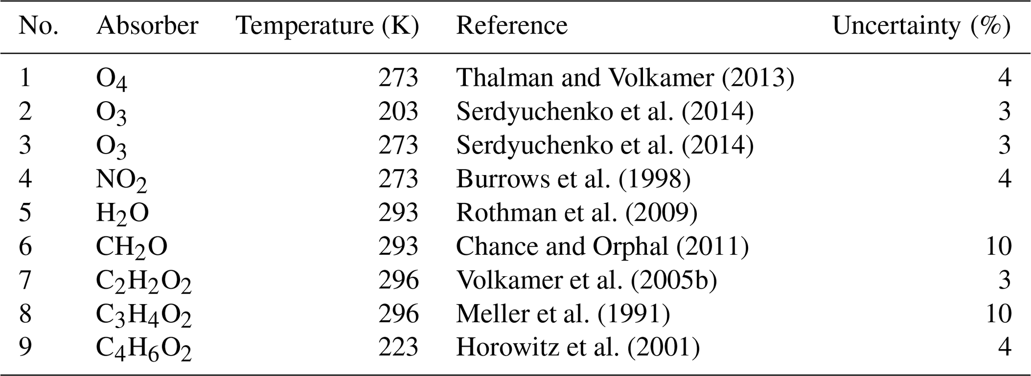
Table 2 Details of the DOAS spectral analysis for the various trace gases.

^a I_Ofs: offset spectrum. ^b R: ring spectrum. ^c R⋅λ⁴: ring spectrum multiplied by λ⁴.

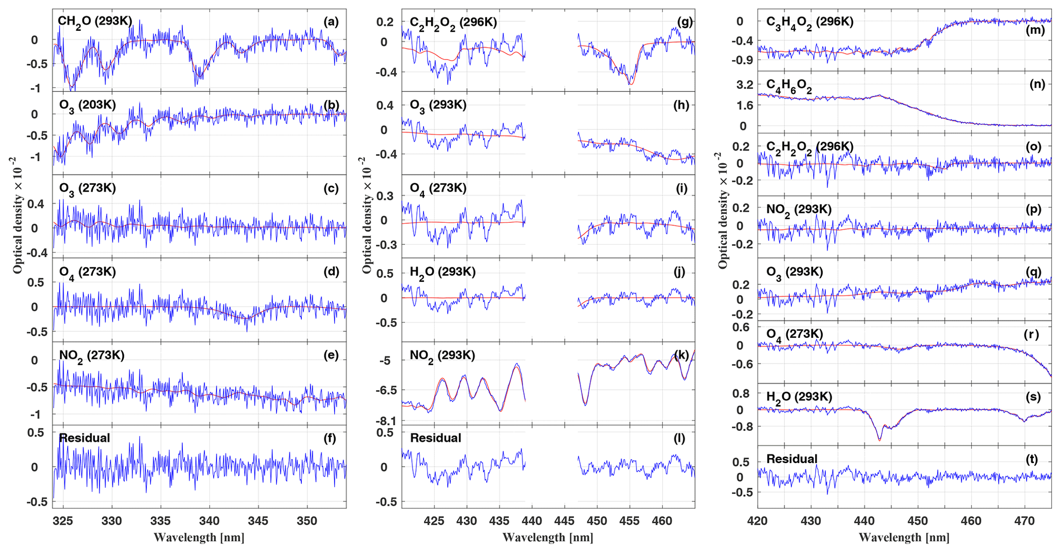
Figure 1 Inferred absorption spectra of CH₂O (a–f), C₂H₂O₂ (g–l), and ${\mathrm{C}}_{\mathrm{3}}{\mathrm{H}}_{\mathrm{4}}{\mathrm{O}}_{\mathrm{2}}^{*}$ (m–t) for the measurements at 17:16, 15:06, and 14:53 UTC, respectively, during the flight on 11 September 2014 (AC11). The traces shown in blue are the inferred atmospheric spectra together with the residual spectral structures; the red line shows the reference spectra of the respective gases. In order to avoid cross correlations with the 7ν absorption band of H₂O at 442 nm, C₂H₂O₂ is simultaneously fitted over two separated spectral windows, ranging from 420 to 439 and 447 to 465 nm.

Exemplary sample retrievals of CH₂O, C₂H₂O₂, and ${\mathrm{C}}_{\mathrm{3}}{\mathrm{H}}_{\mathrm{4}}{\mathrm{O}}_{\mathrm{2}}^{*}$ are shown in Fig. 1. The detection of ${\mathrm{C}}_{\mathrm{3}}{\mathrm{H}}_{\mathrm{4}}{\mathrm{O}}_{\mathrm{2}}^{*}$ (Fig. 1m–t) deserves a brief discussion. It is known that substituted dicarbonyls such as biacetyl (CH₃COCOCH₃), with absorption cross sections in the visible spectral range similar to those of C₃H₄O₂, are also co-emitted from biomass fires in significant quantities (e.g. Meller et al., 1991; Horowitz et al., 2001; Thalman et al., 2015; Zarzana et al., 2017). Owing to the moderate resolution of our spectrometer in the visible spectral range (full width at half maximum resolution of 1.1 nm or 8.4 pixels; see Hüneke, 2016), we cannot separately (and thus unambiguously) detect these substituted dicarbonyls in the atmosphere, unlike in studies employing higher resolving spectrometers (e.g. Thalman et al., 2015). Accordingly, we report here the weighted sum (absorption cross section times concentration) of C₃H₄O₂ and that of other substituted dicarbonyls and express that quantity as ${\mathrm{C}}_{\mathrm{3}}{\mathrm{H}}_{\mathrm{4}}{\mathrm{O}}_{\mathrm{2}}^{*}$.

From the retrieved slant column densities, absolute concentrations of the targeted gases are inferred using the recently developed O₄ scaling method. As shown in previous studies, the scaling method is based on simultaneous measurements of the target gas X and a scaling gas P of known concentration (here the collision complex O₂−O₂, briefly called O₄) in the same wavelength interval (Hüneke, 2016; Hüneke et al., 2017; Stutz et al., 2017; Werner et al., 2017). From the mini-DOAS limb measurements of the total slant column density, the concentration [X]_j of the trace gas X in the atmospheric layer j (i.e. the altitude of the aircraft) is then determined from

$$\begin{array}{}\text{(1)}& [\mathrm{X}{]}_j={\displaystyle \frac{{\mathit{\alpha }}_{X_j}}{{\mathit{\alpha }}_{P_j}}}\cdot {\displaystyle \frac{{\mathrm{SCD}}_X}{{\mathrm{SCD}}_P}}\cdot [P{]}_j\end{array}$$

(see Stutz et al., 2017, Eq. 14). Here, [P]_j is the calculated extinction of O₄ (${\mathit{ϵ}}_{{\mathrm{O}}_{\mathrm{4}}}=\mathit{\sigma }\cdot k_{\mathrm{eq}}\cdot {\left[{\mathrm{O}}_{\mathrm{2}}\right]}_j^{\mathrm{2}}$) in the atmospheric layer j, from which we take the sample. SCD_P is the measured optical depth of O₄, and SCD_X is the measured slant column density of the target gas X. The α-factors ${\mathit{\alpha }}_{X_j}$ and ${\mathit{\alpha }}_{P_j}$ each express the ratio of the absorption of the gas in layer j to the total atmospheric absorption. Usually, the α-factors are simulated in supporting radiative transfer calculations using the Monte Carlo model McArtim (Deutschmann et al., 2011; Knecht, 2015). When needed, the total atmospheric column density of the respective gases is approximated by integrating the measured lower- and higher-quartile profiles in incremental steps of 100 m each (Fig. 9).

When applying the scaling method to airborne UV–vis spectroscopy in limb geometry, a powerful radiative transfer model is necessary to treat the radiative transfer in 2D or 3D, calculate the refraction, and also account for the sphericity of the Earth. We use the Monte Carlo radiative transfer model McArtim (Deutschmann et al., 2011), where each measurement is modelled forward while considering the actual atmospheric, instrumental, and observational (e.g. Sun position relative to the pointing) parameters; the geolocation; and the pointing of the telescope as described in Hüneke (2016) and Hüneke et al. (2017). Further, a combination of climatological aerosol profiles obtained by LIVAS (Amiridis et al., 2015) and the Stratospheric Aerosol and Gas Experiment II (SAGE II) (https://asdc.larc.nasa.gov/project/SAGE II/SAGE2_AEROSOL_O3_NO2_H2O_BINARY_V7.0, last access: 16 October 2020) is considered. For the calculation of the α-factors, box air mass factors are simulated and summed weighted by concentration (Stutz et al., 2017, Eq. 11). We calculate the extinction [P]_j to obtain the vertical O₄ profile. For the target gases CH₂O, C₂H₂O₂, and ${\mathrm{C}}_{\mathrm{3}}{\mathrm{H}}_{\mathrm{4}}{\mathrm{O}}_{\mathrm{2}}^{*}$, we assume exponentially decaying profiles. The latter appears justified because of photochemical arguments, the source distribution (mostly surface), the photochemical lifetimes, and the timescales of possible vertical transport, as well as when inspecting the profile shapes obtained in the post-analysis (Fig. 9).

Evidently, UV–vis limb measurements naturally divide the atmosphere into three different layers, which are separated by the different contributions to the total absorption or optical depth (OD). These contributions are (a) the overhead absorption (OD_oh), (b) the absorption located within the line of sight of the telescopes (OD_limb) (of which most, but not all, is due to single scattering), and (c) the absorption below the line of sight (OD_ms) (of which the photon paths are necessarily all of higher scattering order). In the following, we discuss the significance of the different contributions exemplarily for O₄. Evidently, the same tri-partitioning applies for all other gases of interest, however differently weighted as expressed by the respective alpha-factors. For a high-flying aircraft, OD_oh has the least uncertainty since O₄ absorption approximately scales with [O₂]², and the optical state of the overhead atmosphere is well known. Therefore, the remainder of the measured total O₄ absorption has to be due to the varying contributions of OD_limb and OD_ms, which are mostly modulated by the current low-level cloud cover and ground albedo (Stutz et al., 2017, Fig. 7). The knowledge of the α-factor however gives a handle on the relative fractions OD_limb and OD_ms, since contribution OD_limb can be calculated from ${\mathrm{OD}}_{\mathrm{limb}}=\mathit{\alpha }\cdot {\mathrm{OD}}_{\mathrm{meas}}$, and accordingly ${\mathrm{OD}}_{\mathrm{ms}}={\mathrm{OD}}_{\mathrm{meas}}-{\mathrm{OD}}_{\mathrm{oh}}-{\mathrm{OD}}_{\mathrm{limb}}$. Still, the calculated attributions of OD_limb and OD_ms to OD_meas can only be approximated due to the assumptions made regarding the current aerosol distribution and the cloud coverage.

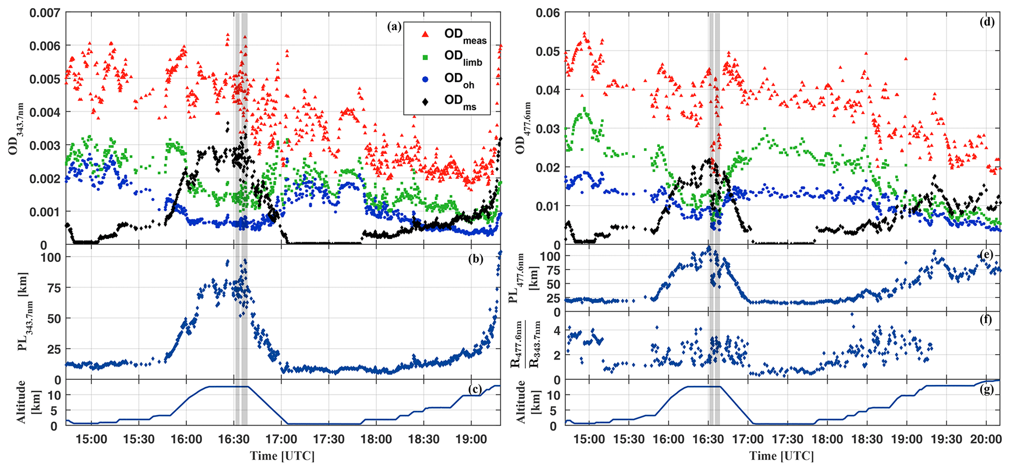
Figure 2 Attribution of the total measured optical depth of O₄ at 343.7 nm (a–c) and at 477.6 nm (d–g) to the various fractions, i.e. absorption from overhead at the aircraft (OD_oh), from multiple scattering below the aircraft (OD_ms), within the line of sight of the telescopes (OD_limb), and the total measured optical depth of O₄ (OD_meas) for the HALO flight on 16 September 2014 (AC11) (a, d). The average line-of-sight photon path length inferred from the measured OD_meas at 343.7 and 477.6 nm, respectively, as a function of the flight time is plotted in (b, e). The colour ratio $\frac{R_{\mathrm{343.7}}}{R_{\mathrm{477.6}}}$ of the measured radiances at 343.7 versus 477.6 nm is shown in (f). The flight trajectory of the HALO aircraft is shown in (c, g). The sharp drop of the optical depth between 16:32–16:3 and 16:35–16:39 UTC (grey bars) coincides with the passage of a cumulonimbus cloud in front of the telescopes. For details see the text.

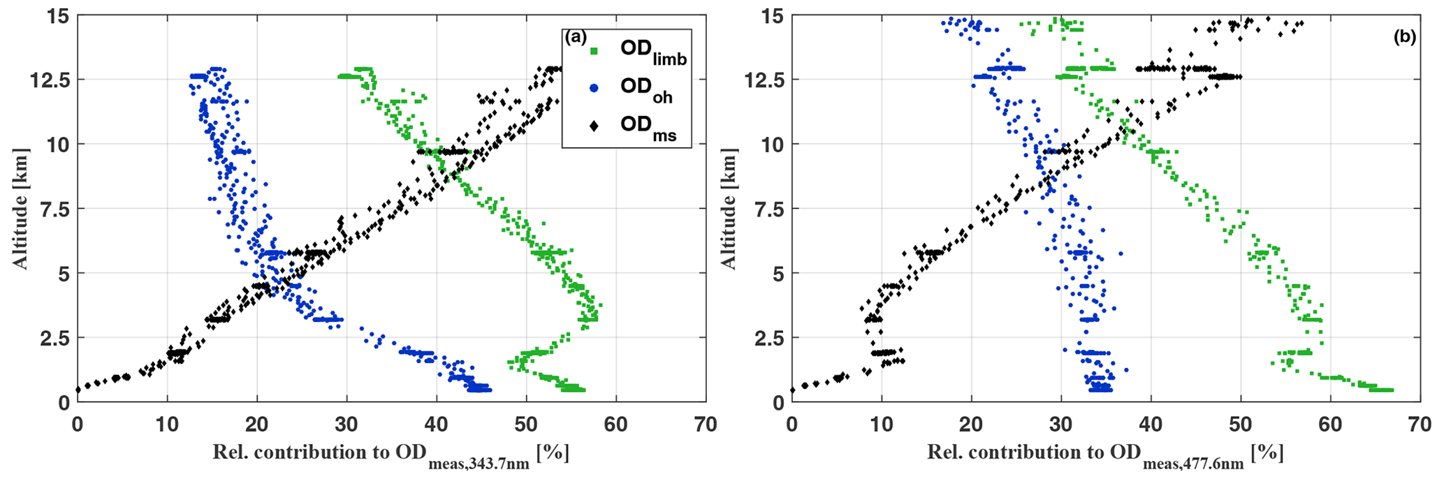
Figure 3 Relative contribution to the limb measured optical depth of O₄ at 343.7 nm (a) and at 477.6 nm (b) due to the absorption overhead of the aircraft (OD_oh), from multiple scattering (OD_ms), and within the line of sight of the telescopes (OD_limb) for the HALO flight on 11 September 2014 (AC11). For details see the text.

Figure 2 illustrates the contributions to OD_meas at 343.7 nm (panel a) and 477.3 nm (panel d) for O₄ as a function of the flight time for 16 September 2014. Figure 3 shows the same data, but sorted by flight altitude to demonstrate the relative change of the contributions. Up to 10 km altitude and for both investigated wavelengths, the absorption within the line of sight of the telescopes contributes with more than 50 % to the total O₄ absorption. A relative minimum can be seen at the top of the planetary boundary layer at approximately 2 km, where often stratocumulus clouds prevail over the Amazon. Further, a maximum of OD_limb is visible at about 4 km, most probably a result of the increasing horizontal visibility with altitude and the moderate contribution of reflected multiple scattered photons from the lower atmosphere to the total O₄ absorption. In the upper troposphere, the relative contribution of OD_limb to OD_meas decreases while the effective horizontal light paths become longer and reach maximum values around 100 km. But given all uncertainties in the details of the actual atmospheric aerosol content, the cloud structure and coverage, and their optical properties, it is more reasonable to speak here of an indication rather than a determination of the photon path lengths.

Fortunately, these uncertainties do not propagate into the uncertainty of the α-factor ratio and hence into the determination of [X]_j, provided the gases X and P have similar profile shapes (Knecht, 2015; Hüneke et al., 2017; Stutz et al., 2017). From the above discussion, it also becomes clear that our air-borne UV–vis limb measurements average over some atmospheric volume, which is determined by the viewing angle of the telescope lenses (0.3°), the light path length, and the aircraft displacement during the time of measurement, both of which are on the order of several kilometres (for details see Sect. 3 and Fig. 6). This large sampling volume precludes direct comparisons with in situ-measured quantities on spatial scales smaller than the current averaging volume. This is of relevance to our study, for example when adding information from in situ measurements like CO to the analysis of our data.

Summing up all described uncertainties, the precision error of the combined methods can be approximately calculated according to Eq. (1) as

$$\begin{array}{}\text{(2)}& \begin{array}{rl}& {\left[\mathrm{\Delta }X\right]}_j=\\ & \sqrt{{\left({\displaystyle \frac{\mathrm{\Delta }{\mathit{\alpha }}_{R,j}}{{\mathit{\alpha }}_{R,j}}}\right)}^{\mathrm{2}}+{\left({\displaystyle \frac{\mathrm{\Delta }{S}_{X,j}}{S_{X,j}}}\right)}^{\mathrm{2}}+{\left({\displaystyle \frac{\mathrm{\Delta }{S}_{P,j}}{S_{P,j}}}\right)}^{\mathrm{2}}+{\left({\displaystyle \frac{\mathrm{\Delta }{P}_j}{P_j}}\right)}^{\mathrm{2}}}\\ & \cdot {\left[X\right]}_j,\end{array}\end{array}$$

where Δα_R, j accounts for (a) random Mie extinction, (b) small-scale variability of the target and scaling gas mixing ratios at flight level, and (c) uncertainty in the sampling contribution as discussed in Figs. 2 and 3. The slant column errors ΔS_X, j and ΔS_P, j account for (a) uncertainty of the inferred Fraunhofer reference slant column density (SCD) and (b) the DOAS fit error. ΔP_j accounts for the uncertainty of the in situ mixing ratio of the scaling gas, which in the case of O₄ scales with the air density and is accordingly limited by the measurement uncertainty of pressure and temperature. Additionally, the systematic errors of the individual absorption cross sections need to be added to ΔS_X, j according to Table 1. An extensive discussion of the total error budget of the O₄ scaling can be found in Hüneke (2016). While ΔP_j and Δα_R, j contribute approximately constantly to the total error budget, ΔS_X, j strongly increases with decreasing slant column density. For mixing ratios below 1 ppb (CH₂O), 0.15 ppb (C₂H₂O₂), and 1.3 ppb (${\mathrm{C}}_{\mathrm{2}}{\mathrm{H}}_{\mathrm{4}}{\mathrm{O}}_{\mathrm{2}}^{*}$), the total precision error is strongly dominated by ΔS_X, j. For higher mixing ratios, Δα_R, j and ΔS_X, j contribute in equal parts in the cases of C₂H₂O₂ and ${\mathrm{C}}_{\mathrm{2}}{\mathrm{H}}_{\mathrm{4}}{\mathrm{O}}_{\mathrm{2}}^{*}$. For CH₂O, Δα_R, j is the major error factor for mixing ratios above 1 ppb, and ΔS_X, j only makes up 30 % of the total error. For all gases, ΔP_j never exceeds 7 % of the total precision error. Due to the strong dependence of ΔS_X, j on the slant column density and the exponentially decreasing vertical profiles of the gases, the resulting total precision errors [ΔX]_j are strongly altitude dependent (Fig. 4).

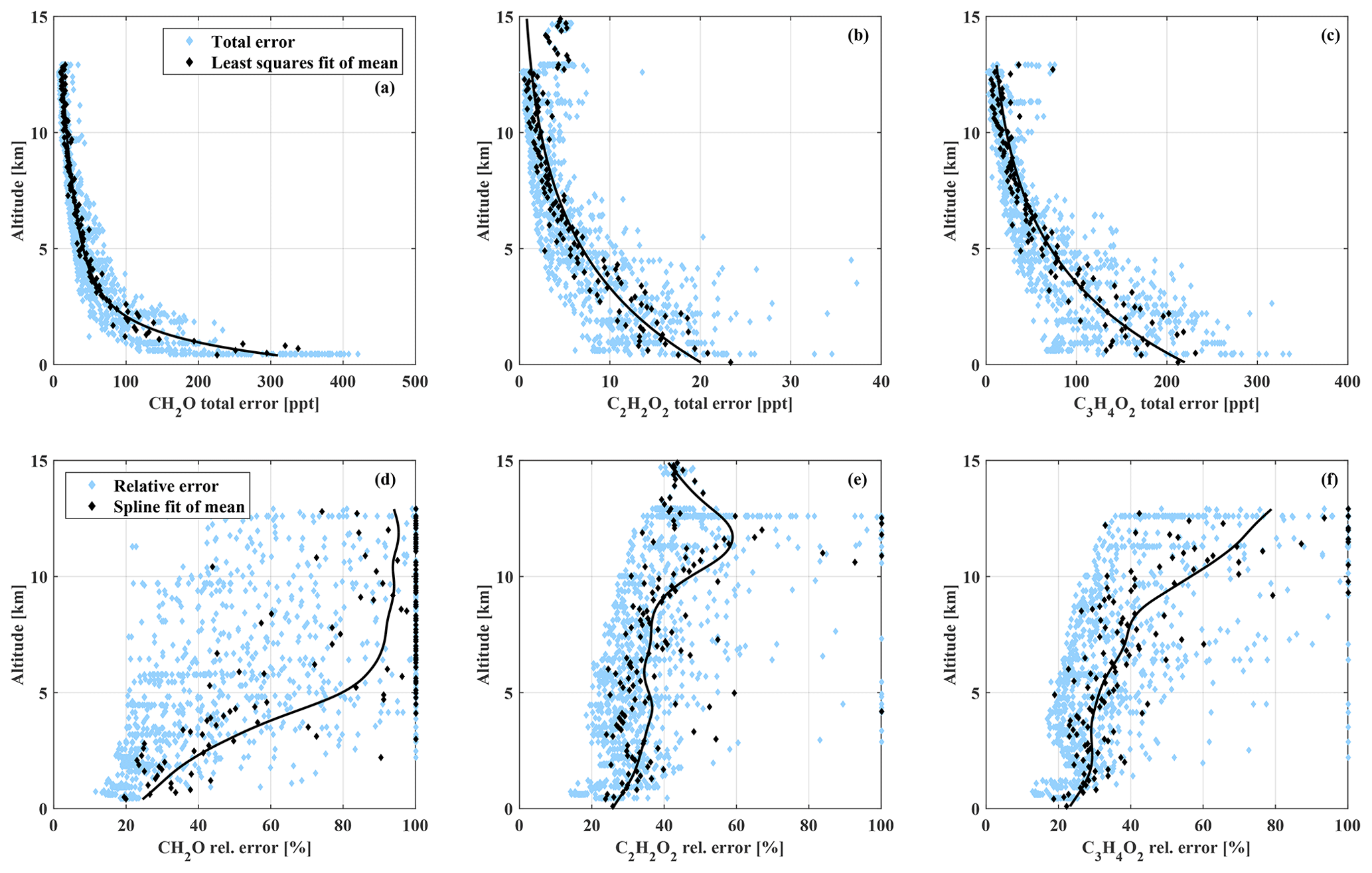
Figure 4 Relative and absolute total precision error of all measurements as a function of the measurement altitude.

They range from 16 % to 100 % for CH₂O, 17 % to 100 % for C₂H₂O₂, and 16 % to 100 % for ${\mathrm{C}}_{\mathrm{2}}{\mathrm{H}}_{\mathrm{4}}{\mathrm{O}}_{\mathrm{2}}^{*}$. This study focuses on measurements below 2 km altitude, with mean total errors of the analysed biomass burning events on the order of 21 % for CH₂O (upper and lower limits of the total precision errors are 350 and 740 ppt), 25 % for C₂H₂O₂ (total errors from 30 to 45 ppt), and 22 % for ${\mathrm{C}}_{\mathrm{2}}{\mathrm{H}}_{\mathrm{4}}{\mathrm{O}}_{\mathrm{2}}^{*}$ (total errors from 240 to 560 ppt).

2.2 AMTEX CO measurements

In situ CO measurements were performed using an Aero-Laser 5002 vacuum UV resonance fluorescence instrument (Gerbig et al., 1996, 1999) installed in the cabin of the HALO aircraft. The main components of the CO instrument include a fluorescence chamber, resonance lamp, optical filter, two dielectric mirrors, and a pump. Atmospheric air is sampled through a backward-facing inlet mounted on top of the HALO fuselage. CO molecules in the ambient air are excited in the chamber by radiation from a radio frequency discharge resonance lamp. The wavelength range (centreline 151 nm with a bandwidth of 9 nm) is selected by the optical filter and the mirrors. The fluorescence signal is detected by a photomultiplier. The flow rate of the sample air through the fluorescence chamber is set to 40 mL min⁻¹ (STP). The sample air is dried with a SICAPENT trap (granulated phosphorus pentoxide drying agent) to eliminate a cross sensitivity to water vapour.

The CO measurements are made at 1 Hz with a precision of 1.5 ppb. The accuracy is given by the precision and systematic errors caused by the drift of the background signal and sensitivity of the instrument and the uncertainty of the CO calibration standard. The total accuracy amounts to 1.5 ppb±2.4% (Gerbig et al., 1999). The CO instrument has been deployed during many aircraft campaigns using the DLR Falcon (e.g. Huntrieser et al., 2016a, b) and was used for the first time on board HALO during the ACRIDICON-CHUVA campaign (Wendisch et al., 2016).

3 Measurements

The ACRIDICON-CHUVA aircraft campaign took place from the operational basis Manaus (Brazil) within the period of September and early October 2014 with a total of 14 scientific flights over the Amazon region. An overview of all ACRIDICON-CHUVA flight tracks can be found in Wendisch et al. (2016), Fig. 6. The campaign aimed to improve the understanding of tropical deep convective clouds and their interaction with biogenic and anthropogenic aerosols, and it also included precipitation formation and air pollution studies. A detailed description of the campaign objectives and the participating instruments and research groups is given in Wendisch et al. (2016).

Our study requires simultaneous measurements of CH₂O, C₂H₂O₂, ${\mathrm{C}}_{\mathrm{3}}{\mathrm{H}}_{\mathrm{4}}{\mathrm{O}}_{\mathrm{2}}^{*}$, and O₄ (performed by the mini-DOAS spectrometers in the UV and visible spectral ranges as described in Sect. 2.1) as well as CO measurements (performed by the AMTEX instrument; see Sect. 2.2), but the instruments occasionally failed. Therefore, only for a subset of flights are joint data available. Further, since a part of the flights focused on objectives other than near-surface air pollution, here we only present data from four out of the 14 ACRIDICON-CHUVA flights, i.e. those on 11 (AC09), 16 (AC11), 18 (AC12), and 19 (AC13) September 2014. Nevertheless, the data collected during these flights provide valuable information on the different measured pollutants, their sources, atmospheric transformation and transport in pristine background air in the troposphere, and fresh and aged air affected by biomass burning in the Amazon.

Each of these measurement flights took 7–8 h, typically occurring between 14:00 and 22:00 UTC, i.e. during daytime. The long flight time supported the sampling of a large geographical area of the rain forest during the four flights, reaching from approximately 6^∘ S to 8^∘ N and 49 to 63^∘ W. The detailed flight tracks and respective altitudes are shown in Fig. 5.

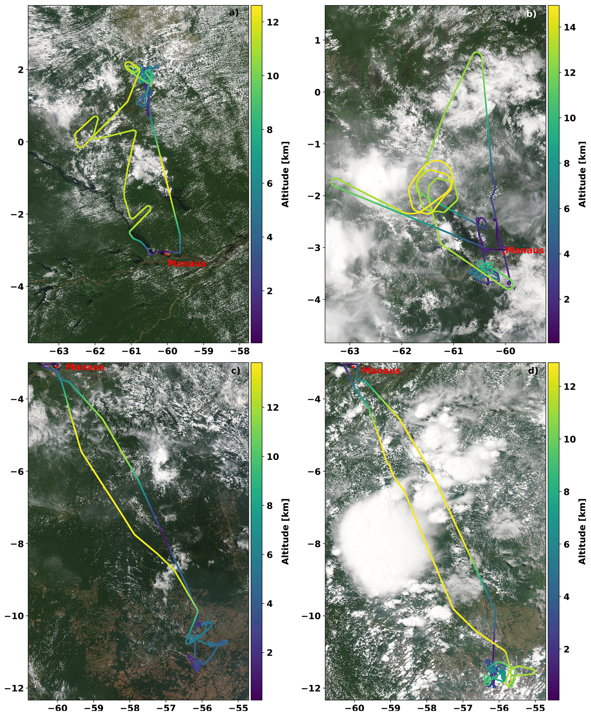
Figure 5 Tracks of the ACRIDICON-CHUVA flights (a) on 11 September 2014, (b) on 16 September 2014 (AC11), (c) on 18 September 2014 (AC12), and (d) on 19 September 2014 (AC13). All flights started and ended at the operational base Manaus airport in Brazil (red dot). The colour coding indicates the flight altitude. The MODIS satellite images are from 14:10 UTC (11 September 2014), 14:30 UTC (16 September 2014), 14:20 UTC (18 September 2014), and 17:55 UTC (19 September 2014). The images were taken from NASA Worldview (https://worldview.earthdata.nasa.gov/, last access: 16 October 2020).

During each of these flights, the probed altitudes ranged from several hundred metres up to 15 km, with flight sections inside the planetary boundary layer overpassing large agricultural areas (AC12 and AC13) as well as the rain forest and the Amazon River delta (AC09 and AC11, Fig. 5).

Due to the relatively large but patchy cloud cover over the Amazon, the UV and vis limb radiances varied significantly during the flights. Therefore, typical integration times of the measured co-added sets of skylight spectra range from seconds (under clear-sky conditions) to several minutes (during cloudy-sky and hazy conditions). In consequence, the along-track resolution of the measurements was typically several kilometres in addition to the horizontal resolution perpendicular to the aircraft determined by radiative transfer (Sect. 2.1). For the biomass burning events AC11-1 to AC11-3 (Table 3 and Sect. 5.4), a two-dimensional visualization of the resulting averaging (or probed) areas per single measurement is indicated by the blue areas in Fig. 6.

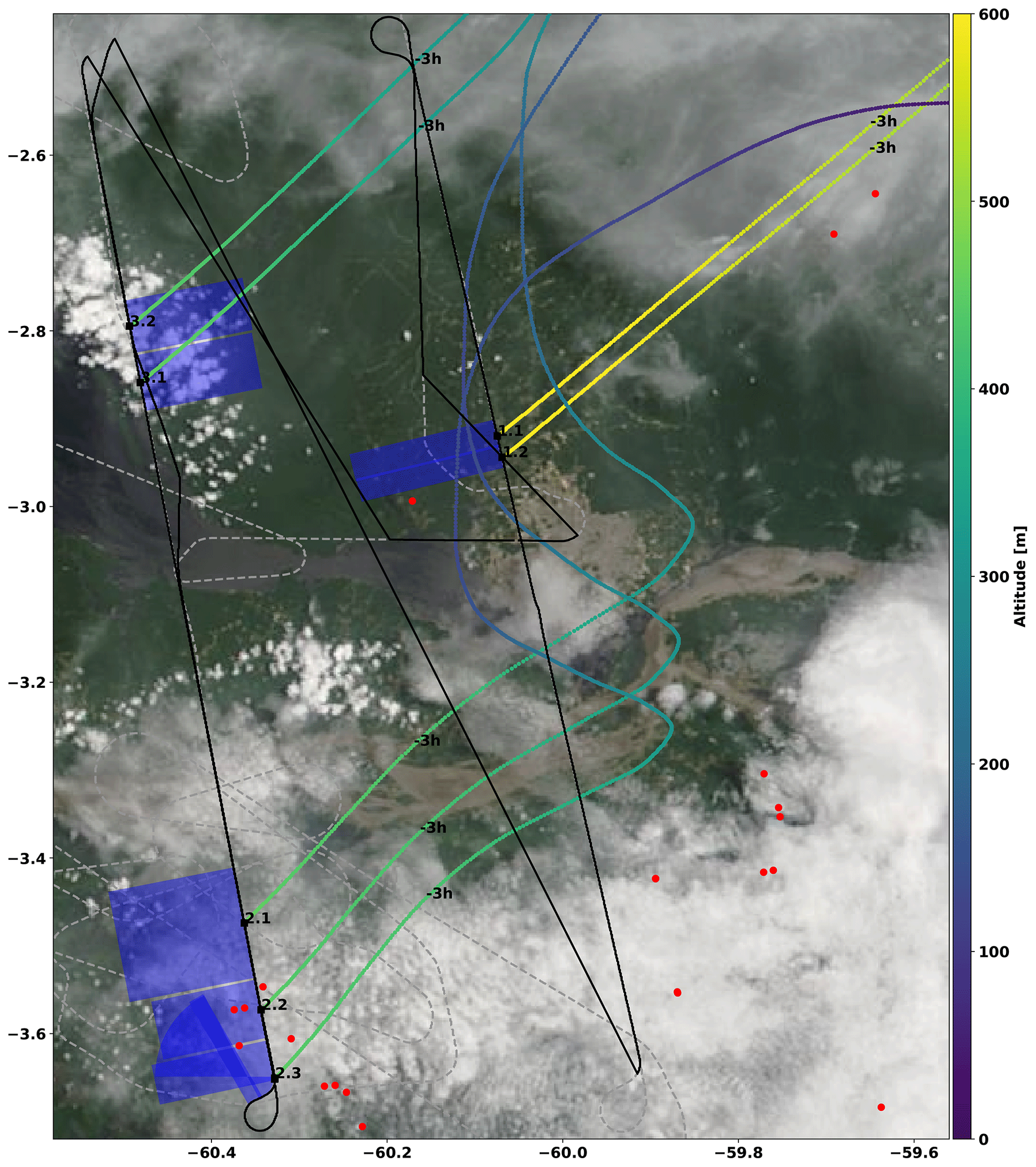
Figure 6 Zoom of the flight track for AC11 on 16 September 2014. The flight tracks below and above 1000 m altitude are labelled by drawn and dashed lines, respectively. The take-off and landing of the aircraft was from Manaus airport (3.1^∘ S, 60.0^∘ W) located in the centre of the image. The biomass burning events detected by the MCD14 MODIS instrument on the Terra and Aqua satellites are indicated with red dots (not to scale). The biomass events probed by the mini-DOAS instrument are marked by black numbers next to the flight track, according to the labelling of Table 3. The blue rectangles approximately indicate the probed air masses in the horizontal plane, where the distance perpendicular to the flight track is given by the O₄ estimated photon path lengths (14 to 19 km) and the along-track distance (3 to 15 km) by the spectrum integration time (33 to 166 s) multiplied by the aircraft ground speed (approximately 95 m s⁻¹) (Sect. 2.1). For each biomass burning event, 3 h backward air mass trajectories were calculated and plotted colour coded by the altitude of the air mass. The MODIS satellite image was taken from NASA WORLDVIEW; see https://worldview.earthdata.nasa.gov/ (last access: 16 October 2020).

The identification of the atmospheric measurement conditions and in particular of each biomass burning event is based on visual imagery using the recorded video data stream (Fig. 7).

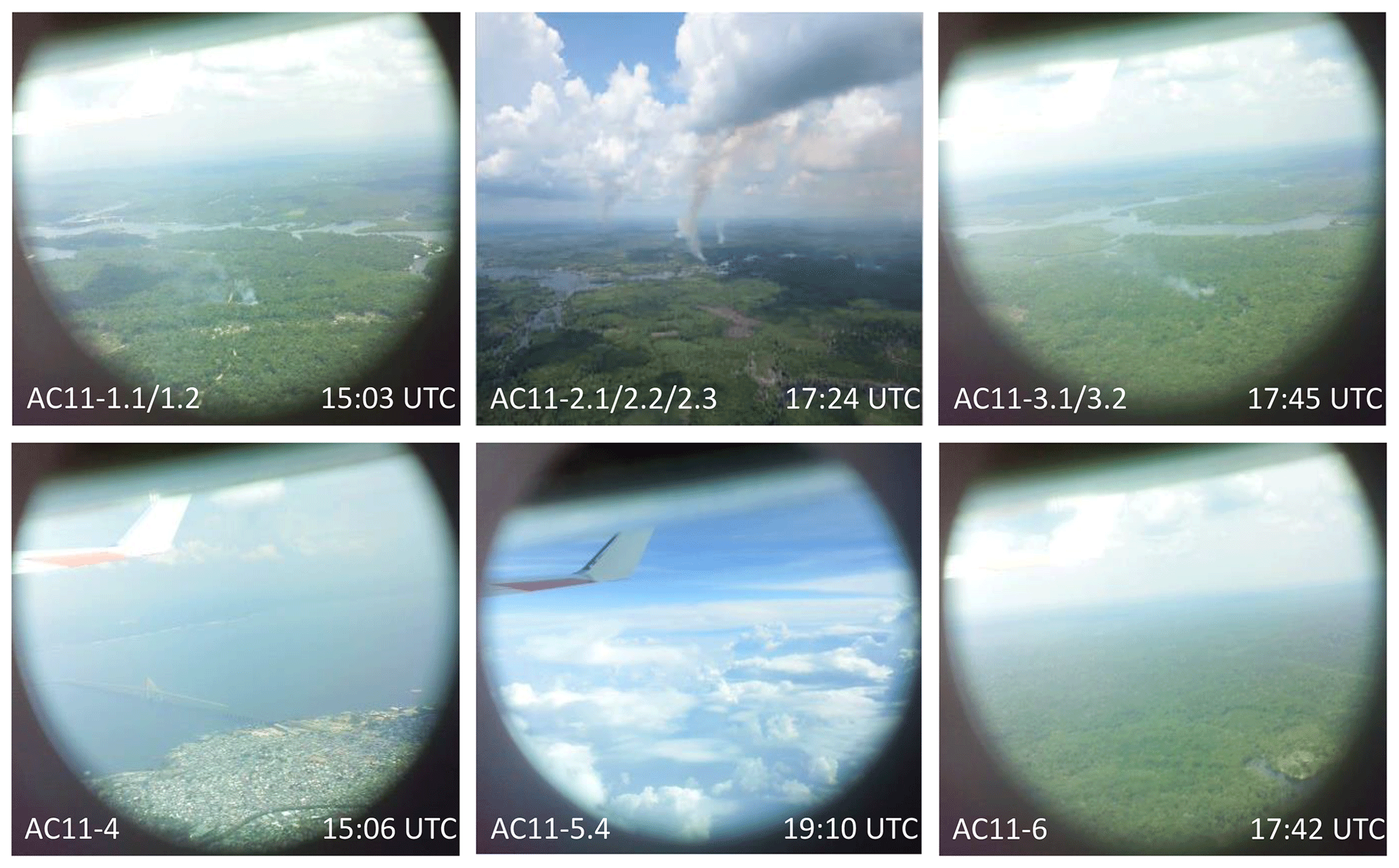
Figure 7 Images taken by the mini-DOAS camera during events 1–6 (as indicated in Figs. 6 and 8) for the flight AC11 with the UTC time given in each image. The second image was taken from the respective flight report. The video camera points in the same direction as the three limb telescopes of the mini-DOAS spectrometer, however with a much larger field of view of $\sim \mathrm{46}{}^{\circ }$ width.

In the following, only those measurements are claimed to be affected by biomass burning, for which the actual plumes are visible in the recorded images and are in the telescope's line of sight. These events are listed in Table 3. Depending on the flight pattern and the integration time of the spectra, some of these plumes were intercepted more than once. In total, eight distinct plumes were probed during 12 individual measurements, all of which were recorded below 2 km flight altitude.

The MODIS instrument on board the Terra and Aqua satellites (MCD14, collection 6, available online from https://worldview.earthdata.nasa.gov/ (last access: 16 October 2020), https://doi.org/10.5067/FIRMS/MODIS/MCD14DL.NRT. 0) reports additional fires in the vicinity of the aircraft trajectory, which were not directly located within the field of view of the mini-DOAS telescopes, nor within the larger field of view of the camera. Therefore, these events are not further investigated in our analysis. However, the emissions of these fires are likely to have created an atmospheric background generally affected by differently aged biomass burning emissions within the boundary layer (Fig. 6). Further insights into the recent photochemical past of the air masses are provided by 3 h backward air mass trajectories calculated using the READY (Real-time Environmental Applications and Display sYstem) website of the NOAA HYSPLIT model (https://www.ready.noaa.gov/HYSPLIT.php, last access: 16 October 2020) (Stein et al., 2015; Rolph et al., 2017). Exemplary 3 h backward trajectories are shown for events AC11-1.2 to AC11-3.2 in Fig. 6. They indicate that prior to detection all air masses resided well within the boundary layer but did not directly pass over any additional reported fire.

However, all identified biomass burning events show large and correlated enhancements of CH₂O, C₂H₂O₂, and ${\mathrm{C}}_{\mathrm{3}}{\mathrm{H}}_{\mathrm{4}}{\mathrm{O}}_{\mathrm{2}}^{*}$, with mixing ratios up to 4.0, 0.26, and 2.8 ppb, respectively (Fig. 8). Due to the differently sized spatial resolutions of both instruments (Sect. 2), the detected peaks in CO and those of CH₂O, C₂H₂O₂, and ${\mathrm{C}}_{\mathrm{3}}{\mathrm{H}}_{\mathrm{4}}{\mathrm{O}}_{\mathrm{2}}^{*}$ do not (and are not expected to) strictly correlate. Therefore, we refrain from directly estimating emission ratios with respect to CO.

4 Results

Figure 8 shows the inferred volume mixing ratios of CH₂O (panel a), C₂H₂O₂ (panel b), ${\mathrm{C}}_{\mathrm{3}}{\mathrm{H}}_{\mathrm{4}}{\mathrm{O}}_{\mathrm{2}}^{*}$ (panel c), and CO (panel d) for flight AC11 on 16 September 2014.

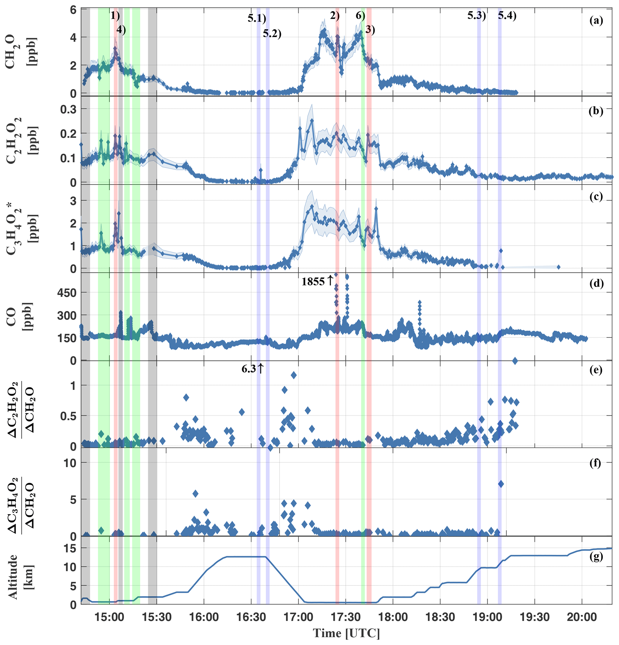
Figure 8 Measured mixing ratios of CH₂O (a), C₂H₂O₂ (b), ${\mathrm{C}}_{\mathrm{3}}{\mathrm{H}}_{\mathrm{4}}{\mathrm{O}}_{\mathrm{2}}^{*}$ (c), CO (d), inferred $R_{\mathrm{GF}}=\mathrm{\Delta }{\mathrm{C}}_{\mathrm{2}}{\mathrm{H}}_{\mathrm{2}}{\mathrm{O}}_{\mathrm{2}}/\mathrm{\Delta }{\mathrm{CH}}_{\mathrm{2}}\mathrm{O}$ (e), $R_{\mathrm{MF}}=\mathrm{\Delta }{\mathrm{C}}_{\mathrm{3}}{\mathrm{H}}_{\mathrm{4}}{\mathrm{O}}_{\mathrm{2}}^{*}/\mathrm{\Delta }{\mathrm{CH}}_{\mathrm{2}}\mathrm{O}$ (f), and the height versus time trajectory for the HALO flight AC11 (g). The shaded blue area in (a–c) shows the respective measurement uncertainty. All measurements within the Manaus city plume are marked by grey bars (e.g. event AC11-4). Examples for measurements in aged air masses of the upper troposphere are marked in blue (e.g. events AC11-5.1–5.4) and green for the general background atmosphere; i.e. tropical-forest-affected air (e.g. event AC11-6). All measurements of biomass burning plumes are labelled in red (events AC11-1, AC11-2, and AC11-3). The event numbers correspond to the labelling in Table 3 and Fig. 7.

The measured trace gas mixing ratios are the largest for flight sections within the planetary boundary layer (14:45 to 15:15 and 17:05 to 17:45 UTC) and the lowest in the upper troposphere (16:15 to 16:45 and 19:15 to 20:20 UTC). Notable are the peaks in CO while flying through the Manaus city plume (grey bars) or biomass burning plumes (red bars). Elevated mixing ratios of CH₂O, C₂H₂O₂, and ${\mathrm{C}}_{\mathrm{3}}{\mathrm{H}}_{\mathrm{4}}{\mathrm{O}}_{\mathrm{2}}^{*}$ can be related to biomass burning as well as to air masses of presumably aged background air (labelled with the green bars) as evidenced by the only moderately elevated CO. Here, the numbers (1) to (6) in panel (a) of Fig. 8 denote biomass-burning-affected air (1–3), air of the Manaus city plume (4), pristine air of the upper troposphere (5), and boundary layer air above the tropical forest (6). Sky images of all six different situations are shown in Fig. 7.

4.1 Vertical profiles

Below 450 m altitude, CO mixing ratios range from 88.6 to 291.8 ppb (Fig. 9, panel a), with a mean of [CO]=188.1 ppb.

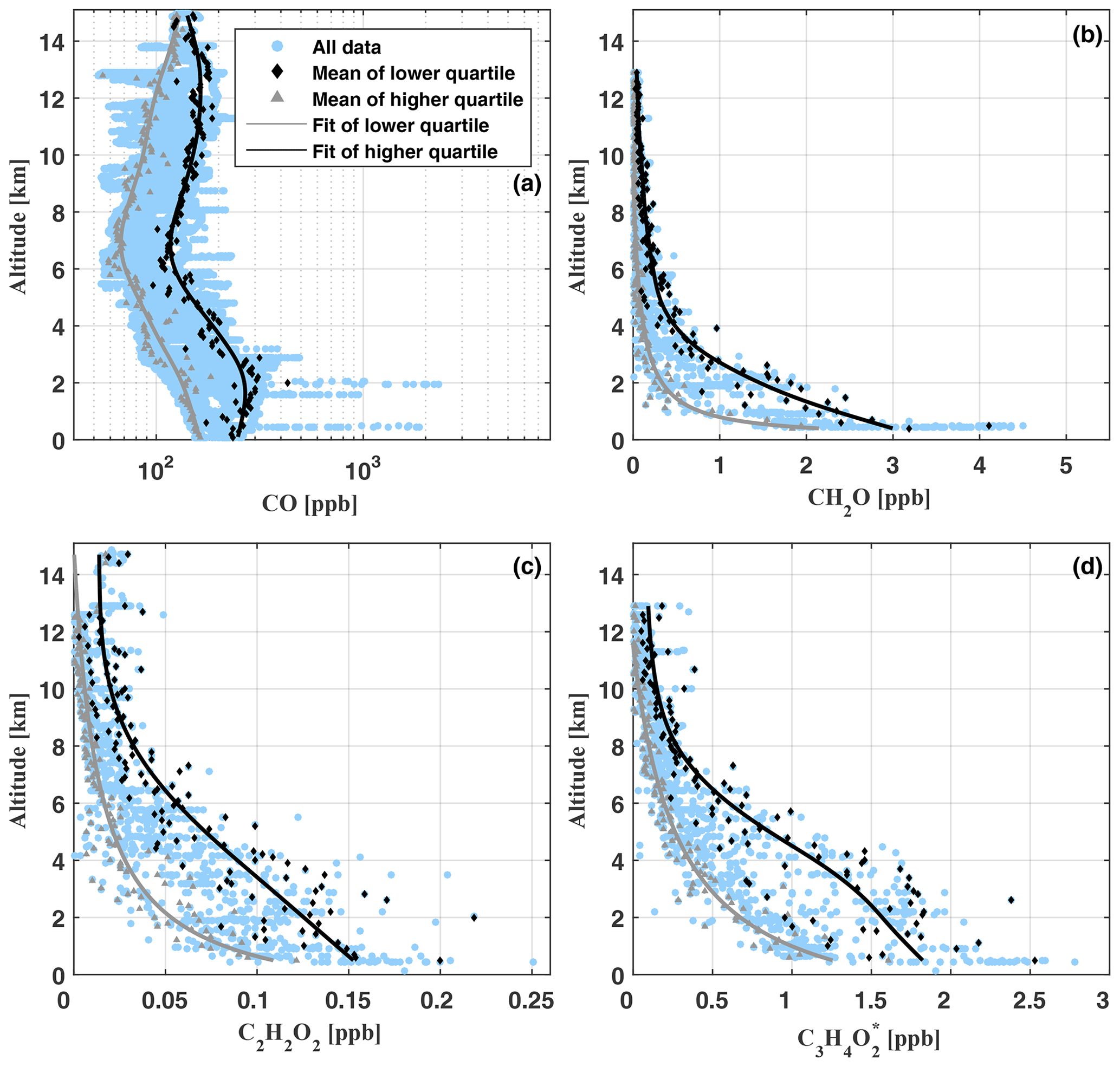
Figure 9 Vertical profiles of CO (a), CH₂O (b), C₂H₂O₂ (c), and ${\mathrm{C}}_{\mathrm{3}}{\mathrm{H}}_{\mathrm{4}}{\mathrm{O}}_{\mathrm{2}}^{*}$ (d) as measured during flights AC09, AC11, AC12, and AC13 (blue circles). Note the logarithmic scale of the x axis in (a). For AC09, there are no CO data available. The grey lines indicate a spline fit (a) and least-squares fits (b–d) through the lower quartile of the data (grey triangles) in 100 m altitude bins. The black lines show corresponding fits through the mean of the upper quartile (black diamonds).

Within the planetary boundary layer, CO mixing ratios increase from 88.4 ppb to 2308 ppb (mean [CO]=212.8 ppb), with peak mixing ratios above 500 ppb appearing when biomass burning plumes are directly passed. The lowest [CO] mixing ratios in the range of 55.1 to 231.9 ppb (mean [CO]=86.3 ppb) are found in the middle troposphere between 6 and 8 km altitude. In the upper troposphere (12–14 km), CO increases from 52.5 to 212.6 ppb (mean [CO]=134.5 ppb). In the convective tropics, C-shaped CO profiles are a well-known phenomenon, caused by the rapid transport of near-surface CO-rich air by mesoscale convective systems into the upper troposphere (e.g. Brocchi et al., 2018; Krysztofiak et al., 2018). When binning the data in 100 m altitude intervals and averaging over the lower and upper data quartiles within each interval, another maximum forms around the top of the boundary layer. Most likely, this suggests that over the Amazon biomass burning plumes often detrain their pollutants near the top of the boundary layer (see for example the image at 17:24 UTC, Fig. 7).

Inferred [CH₂O] ranges from 4.5 ppb near the surface to mean mixing ratios of 30 ppt in the upper troposphere (above 10 km). Mixing ratios within the boundary layer and middle troposphere vary significantly (Fig. 9, panel b). In part, this might be a manifestation of the direct emission of CH₂O into the lower part of the atmosphere or the in situ formation of CH₂O during the oxidation of biogenic VOCs (BVOCs) as well as partly oxidized VOCs (OVOCs). Figure 10 puts our CH₂O measurements over the Amazon into the context of previously published CH₂O observations all over the world. Within this comparison, it is remarkable that the lowest CH₂O mixing ratios measured over the Amazon approximately agree with CH₂O measured within the boundary layer and middle troposphere over the west Pacific by Peters et al. (2012).

Figure 10 Comparison of different CH₂O measurements available from the literature (Arlander et al., 1995; De Smedt et al., 2008; Fried et al., 2008; Dufour et al., 2009; Steck et al., 2008; Boeke et al., 2011; Peters et al., 2012; Kaiser et al., 2015; Chan Miller et al., 2017) with those of the present study (grey). The geographical regions of the measurements are Brazil, South America (SA), North America (NA), west Pacific (WPacific), and MIPAS-Envisat measurements covering orbit 8164, 14^∘ S, 46^∘ W.

Our measurements in the upper troposphere compare well to findings from Dufour et al. (2009) and Boeke et al. (2011) over Brazil and North America, respectively. The lowest mixing ratios measured in the middle and upper troposphere may reflect CH₂O formed during the oxidation of mostly CH₄ and, if available, some residual VOCs, OVOCs, and BVOCs (see Fig. 9, panel c for C₂H₂O₂ and panel d for ${\mathrm{C}}_{\mathrm{3}}{\mathrm{H}}_{\mathrm{4}}{\mathrm{O}}_{\mathrm{2}}^{*}$), since their photochemical and heterogeneous removal is certainly slower than the CH₂O photochemical lifetime of only a few hours (Frost et al., 2002). In contrast, the largest CH₂O mixing ratios measured over the Amazon at any altitude appear slightly smaller than the average and significantly smaller than the maximum mixing ratios reported from the joint SENEX aircraft observations of CH₂O and C₂H₂O₂ over North America (Kaiser et al., 2015; Chan Miller et al., 2017).

C₂H₂O₂ mixing ratios range from 85 to 250 ppt below 500 m altitude and decrease in the upper troposphere (12–14 km) to mixing ratios from 5 ppt (our detection limit) to about 49 ppt. Close to the ground, our results are comparable to C₂H₂O₂ mixing ratios found over North America by Kaiser et al. (2015) and Chan Miller et al. (2017) but much larger than those measured in pristine air masses of the South Pacific (7–23 ppt) by Lawson et al. (2015). Evidently, besides the C₂H₂O₂ formation during the oxidation of BVOCs (Wennberg et al., 2018), a fraction of the near-surface and boundary layer C₂H₂O₂ is certainly due to direct emission by biomass burning (Zarzana et al., 2018; Andreae, 2019). In the middle troposphere, our inferred mixing ratios of C₂H₂O₂ are significantly larger than observations during SENEX (which reach to approximately 6 km altitude) and are also larger in the upper troposphere above 6 km when comparing to data extrapolated from SENEX. Between 6 and 14 km altitude, C₂H₂O₂ enhancements of up to ≈63 ppt become apparent when compared to either the SENEX data or the binned lower quartile of our data. Such elevated mixing ratios of C₂H₂O₂ in the middle and upper troposphere point to an efficient vertical transport of C₂H₂O₂ and its precursors VOCs, OVOCs, and BVOCs from their emission sources at the ground or to direct formation from longer-lived VOCs (e.g. phenols) (Andreae et al., 2001; Taraborrelli et al., 2020). Further, C₂H₂O₂ (and ${\mathrm{C}}_{\mathrm{3}}{\mathrm{H}}_{\mathrm{4}}{\mathrm{O}}_{\mathrm{2}}^{*}$) present at higher atmospheric altitudes may serve as a marker for the formation of ISOPOO (isoprene peroxy radicals), ISOPOOH (oligomer hydroxyhydroperoxides), and finally IEPOX (isoprene epoxydiols) within the isoprene oxidation chain (Wennberg et al., 2018). In fact, IEPOX-mediated SOA formation in the upper troposphere over the Amazon has been reported from observations made within the framework of the ACRIDICON-CHUVA project (Andreae et al., 2018; Schulz et al., 2018).

The detection of ${\mathrm{C}}_{\mathrm{3}}{\mathrm{H}}_{\mathrm{4}}{\mathrm{O}}_{\mathrm{2}}^{*}$, here taken as the sum of methylglyoxal and larger carbonyls as described previously, appears elusive due to the spectral interference among the different species. Weighting of the measured total absorption for ${\mathrm{C}}_{\mathrm{3}}{\mathrm{H}}_{\mathrm{4}}{\mathrm{O}}_{\mathrm{2}}^{*}$ with the relative absorption cross sections of the inferred C₃H₄O₂, C₄H₆O₂ (biacetyl), and C₄C₈O₄ (acetylpropionyl) (Zarzana et al., 2017, Fig. S4) may be indicative of the relative abundance of each species. As in Zarzana et al. (2017), we recommend a weighting factor of 2.0±0.5 by which the inferred ${\mathrm{C}}_{\mathrm{3}}{\mathrm{H}}_{\mathrm{4}}{\mathrm{O}}_{\mathrm{2}}^{*}$ needs to be divided for indicative C₃H₄O₂ mixing ratios. However, we note that the factor of 2.0±0.5 may largely depend on the precursor concentrations, and thus on the geolocation, altitude, and geophysical regime, and therefore barely provides more than a hint on its true size.

Due to the lack of previous atmospheric ${\mathrm{C}}_{\mathrm{3}}{\mathrm{H}}_{\mathrm{4}}{\mathrm{O}}_{\mathrm{2}}^{*}$ (or C₃H₄O₂) measurements, it is more difficult to validate our inferred ${\mathrm{C}}_{\mathrm{3}}{\mathrm{H}}_{\mathrm{4}}{\mathrm{O}}_{\mathrm{2}}^{*}$ profile (Fig. 9, panel d). As for the other measured hydrocarbons, the largest ${\mathrm{C}}_{\mathrm{3}}{\mathrm{H}}_{\mathrm{4}}{\mathrm{O}}_{\mathrm{2}}^{*}$ mixing ratios between 1.2 and 2.8 ppb (mean $\left[{\mathrm{C}}_{\mathrm{3}}{\mathrm{H}}_{\mathrm{4}}{\mathrm{O}}_{\mathrm{2}}^{*}\right]=\mathrm{1.6}\mathrm{ppb}$) are found near the ground and within the planetary boundary layer. Below 1 km altitude, our results of 0.8 to 2.8 ppb (mean $\left[{\mathrm{C}}_{\mathrm{3}}{\mathrm{H}}_{\mathrm{4}}{\mathrm{O}}_{\mathrm{2}}^{*}\right]=\mathrm{1.5}\mathrm{ppb}$) are considerably larger than recently reported C₃H₄O₂ mixing ratios (28 to 365 ppt) from a Mediterranean site with intense biogenic emissions and low levels of anthropogenic trace gases (Michoud et al., 2018), as well as measurements at Cape Grim (28±11 ppt) and the Chatham Rise (10±10 ppt) in pristine marine air (Lawson et al., 2015). Therefore, we expect a major fraction of the enhanced ${\mathrm{C}}_{\mathrm{3}}{\mathrm{H}}_{\mathrm{4}}{\mathrm{O}}_{\mathrm{2}}^{*}$ to be related to the oxidation of BVOCs and biomass burning (e.g. Andreae and Merlet, 2001; Akagi et al., 2011; Stockwell et al., 2015; Zarzana et al., 2017, 2018; Andreae, 2019). Evidence that the former is overall the more relevant process (compared to direct emissions by biomass burning) in the Amazonian troposphere is also provided by the relatively compact clustering of the inferred ${\mathrm{C}}_{\mathrm{3}}{\mathrm{H}}_{\mathrm{4}}{\mathrm{O}}_{\mathrm{2}}^{*}$ along the fit of the lower quartile of the data.

5 Discussion

5.1 Vertical profiles and precursor VOCs

Above the boundary layer, significant enhancements in C₂H₂O₂ and ${\mathrm{C}}_{\mathrm{3}}{\mathrm{H}}_{\mathrm{4}}{\mathrm{O}}_{\mathrm{2}}^{*}$ mixing ratios above the inferred backgrounds are observed (Fig. 9, panels c and d). After applying a correction factor of 2.0±0.5 to the measured ${\mathrm{C}}_{\mathrm{3}}{\mathrm{H}}_{\mathrm{4}}{\mathrm{O}}_{\mathrm{2}}^{*}$ mixing ratios as discussed above, methylglyoxal exceeds the inferred glyoxal mixing ratios by up to a factor of 5 for all measurements. Because of many long flight sections above the remote rain forest, which were to our knowledge at least partly free of fires and plumes, as well as the comparatively different shape of the formaldehyde profile, not all of these enhancements can be attributed to direct emissions from biomass burning.

As their dominant source, isoprene globally accounts for 67 %, 47 %, and 79 % of the annual sources of formaldehyde, glyoxal, and methylglyoxal (Fu et al., 2008), respectively, leading to their rapidly decreasing vertical profiles. As argued by Fu et al. (2008, 2019), the oxidation of isoprene under low-NO_x conditions may be delayed by hours or even several days. This prolonged lifetime combined with the efficient vertical atmospheric transport in the tropics leads to isoprene oxidation above the boundary layer. As a consequence, we suspect the in situ formation of glyoxal and methylglyoxal and finally formaldehyde from isoprene oxidation to contribute significantly to the observed enhanced mixing ratios in the free troposphere. The methylglyoxal enhancements in the middle troposphere are approximately 5 times larger than the observed glyoxal mixing ratios. Molar yields of glyoxal and methylglyoxal from second- and third-generation isoprene oxidation combined are 6.2 % and 34 %, respectively (Fu et al., 2008). Therefore, we expect the in situ formation of methylglyoxal from isoprene oxidation to be approximately 5 times larger than the respective glyoxal production. In accordance with our measurements, this should lead to methylglyoxal mixing ratios that are 5 times larger compared to glyoxal in the free troposphere.

Besides their common dominant precursor, additional sources of the gases differently influence their local distribution (mostly combustion processes and oxidation of other biogenic/anthropogenic hydrocarbons in the case of formaldehyde, Lee et al., 1998; Liu et al., 2007; Fortems-Cheiney et al., 2012; oxidation of acetylene in the case of glyoxal, and oxidation of acetone in the case of methylglyoxal, Fu et al., 2008) and might therefore differently contribute to our measurements. A recent study additionally discussed the oxidation of aromatics as a possible relevant source of atmospheric glyoxal and methylglyoxal (Taraborrelli et al., 2020). While acetylene is mostly an anthropogenically emitted trace gas, acetone additionally has direct biogenic sources. Both gases have a long lifetime of up to 18 and 22 d, respectively (Fu et al., 2008). Therefore, vertically transported acetylene from ground-based combustion processes might be a further source of the observed glyoxal production in the free troposphere. While acetone is also emitted in biomass burning processes (one-fifth of the total acetone budget; Pöschl et al., 2001), an equally large source of acetone emissions is decomposing plant material (${\mathrm{10}}^{-\mathrm{4}}\mathrm{g}{\mathrm{g}}^{-\mathrm{1}}$; Warneke et al., 1999). The remaining acetone is to a large part an oxidation product of hydrocarbons and also an oxidation product of isoprene under low-NO_x conditions, which are typical for air above rain forests (Warneke et al., 2001). Mean acetone mixing ratios in the boundary layer above tropical rain forests are on the order of 2 ppb (Pöschl et al., 2001). Besides isoprene oxidation, a fraction of the observed methylglyoxal enhancements in the free troposphere might therefore be a direct or secondary (through the oxidation of hydroacetone) product of acetone oxidation above the boundary layer or a result of longer-lived oxidized aromatics (Taraborrelli et al., 2020).

It is remarkable that even though formaldehyde, glyoxal, and methylglyoxal have a common dominant source (isoprene) and sink (photolysis), the relative profile shapes are different. Especially above the boundary layer, the inferred formaldehyde mixing ratios decrease faster with increasing altitude than the vertical profiles of glyoxal and methylglyoxal do (Fig. 9, panel b). It should therefore be questioned whether the relative contribution of the different precursor gases, their sinks due to photolysis, and reaction with OH radicals in low-NO_x, high-VOC, and low-HO_x environment, or the different efficiencies regarding the uptake into aerosols or cloud particles may alter the relative profile shapes of the three species. The water solubility of the gases is largely different (${\mathrm{H}}^{\mathrm{cp}}=\mathrm{32}\mathrm{mol}{\mathrm{m}}^{-\mathrm{3}}{\mathrm{Pa}}^{-\mathrm{1}}$ for formaldehyde, ${\mathrm{H}}^{\mathrm{cp}}=\mathrm{4100}\mathrm{mol}{\mathrm{m}}^{-\mathrm{3}}{\mathrm{Pa}}^{-\mathrm{1}}$ for glyoxal, and ${\mathrm{H}}^{\mathrm{cp}}=\mathrm{370}\mathrm{mol}{\mathrm{m}}^{-\mathrm{3}}{\mathrm{Pa}}^{-\mathrm{1}}$ for methylglyoxal; see Sander, 2015) and significantly smaller for formaldehyde than glyoxal. Heterogeneous uptake may therefore not provide an explanation for the relative depletion of formaldehyde over glyoxal and methylglyoxal in the middle troposphere.

5.2 Comparison with satellite measurements

As neither CH₂O nor C₂H₂O₂ have relevant stratospheric sources, the integration of the profiles yields their total vertical column density (VCD). The uncertainty of the integrated profiles follows from the altitude-weighted total error of our measurements as displayed in Fig. 4. We compare our findings to measurements from GOME (Global Ozone Monitoring Experiment), SCIAMACHY (SCanning Imaging Absorption spectroMeter for Atmospheric CHartographY), OMI (Ozone Monitoring Instrument), and GOME-2, which combined provide global CH₂O and C₂H₂O₂ observations covering more than a decade (Fig. 11).

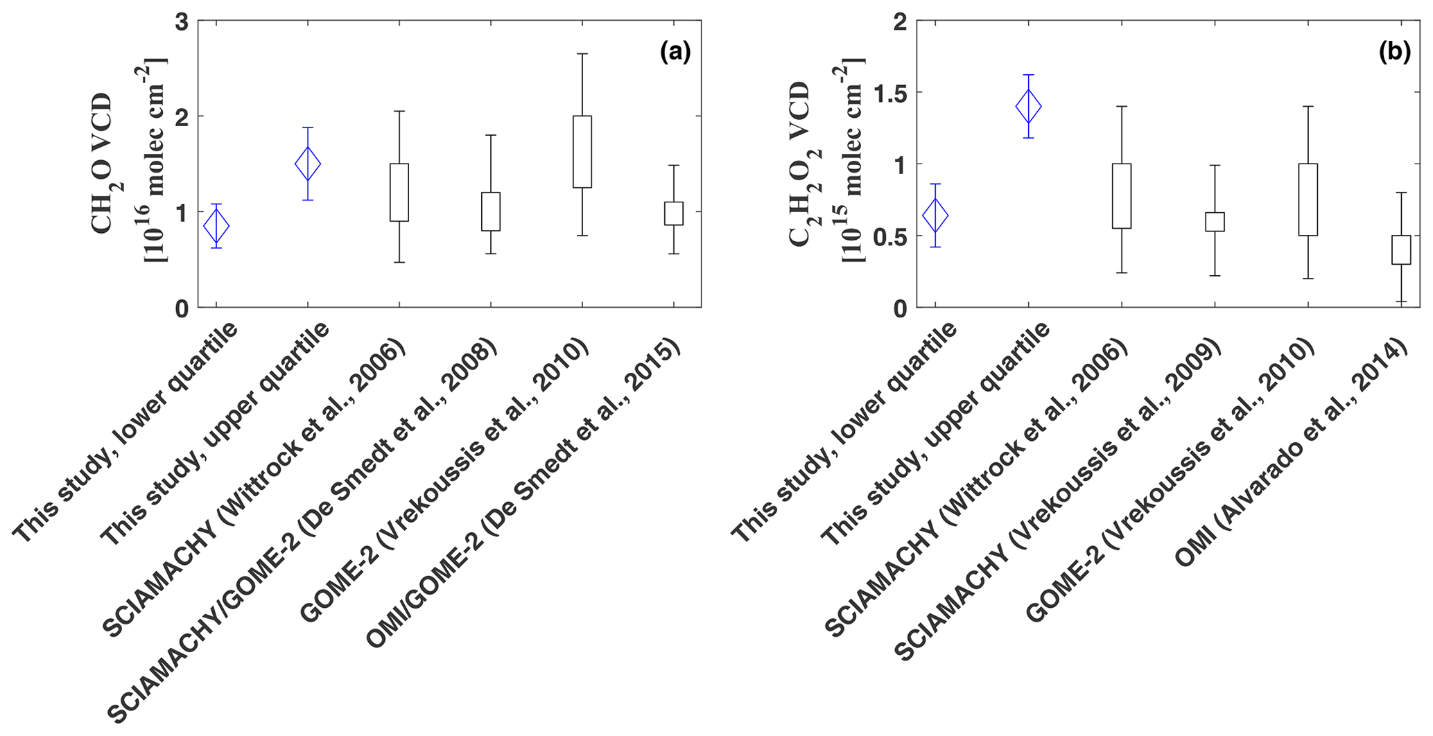
Figure 11 Comparison of the integrated total column densities of CH₂O (a) and C₂H₂O₂ (b). The vertical bars indicate the range of the observed vertical column amounts as reported in the respective studies. The uncertainty range for Wittrock et al. (2006) and Alvarado et al. (2014) was estimated based on Vrekoussis et al. (2009).

Integration of the CH₂O profiles yields total column densities of $\left(\mathrm{0.9}\pm \mathrm{0.2}\right)\times {\mathrm{10}}^{\mathrm{16}}\mathrm{molec}.{\mathrm{cm}}^{-\mathrm{2}}$ (lower quartile as plotted in Fig. 9) to $\left(\mathrm{1.5}\pm \mathrm{0.4}\right)\times {\mathrm{10}}^{\mathrm{16}}\mathrm{molec}.{\mathrm{cm}}^{-\mathrm{2}}$ (upper quartile), with a mean of $\left(\mathrm{1.1}\pm \mathrm{0.3}\right)\times {\mathrm{10}}^{\mathrm{16}}\mathrm{molec}.{\mathrm{cm}}^{-\mathrm{2}}$ (all data, Fig. 11, panel a). Satellite observations generally report enhanced CH₂O VCDs over regions with large biogenic emissions, especially over the Amazon Basin, with maximal enhancements during the dry season. Monthly means of CH₂O VCDs measured by GOME and SCIAMACHY in the years 1996–2007 over the Amazon report maximal enhancements of 1–$\mathrm{2}\times {\mathrm{10}}^{\mathrm{16}}\mathrm{molec}.{\mathrm{cm}}^{-\mathrm{2}}$ during the dry season and much smaller vertical column densities of $\mathrm{0.8}\times {\mathrm{10}}^{\mathrm{16}}\mathrm{molec}.{\mathrm{cm}}^{-\mathrm{2}}$ during the wet season (De Smedt et al., 2008). Our inferred CH₂O vertical column densities based on the lower quartile agree well with their measurements during the wet season, while our integrated profile of the upper quartile lies within the observations during the dry season. Our results agree equally well with SCIAMACHY observations in 2005 over South America with an annual mean CH₂O VCD of approximately $\mathrm{1.2}\times {\mathrm{10}}^{\mathrm{16}}\mathrm{molec}.{\mathrm{cm}}^{-\mathrm{2}}$ as reported by Wittrock et al. (2006) and also agree with GOME-2 observations, for which Vrekoussis et al. (2010) report CH₂O VCDs of 1.2 to $\mathrm{1.6}\times {\mathrm{10}}^{\mathrm{16}}\mathrm{molec}.{\mathrm{cm}}^{-\mathrm{2}}$ over the Amazon Basin for the years 2007 to 2008. Finally, yearly averaged CH₂O from OMI and GOME-2 observations over Brazil between 2007 and 2013 by De Smedt et al. (2015) agree with our mean of $\mathrm{1.1}\times {\mathrm{10}}^{\mathrm{16}}\mathrm{molec}.{\mathrm{cm}}^{-\mathrm{2}}$.

The integrated C₂H₂O₂ profiles range from $\left(\mathrm{0.6}\pm \mathrm{0.2}\right)\times {\mathrm{10}}^{\mathrm{15}}\mathrm{molec}.{\mathrm{cm}}^{-\mathrm{2}}$ (lower quartile) to $\left(\mathrm{1.4}\pm \mathrm{0.4}\right)\times {\mathrm{10}}^{\mathrm{15}}\mathrm{molec}.{\mathrm{cm}}^{-\mathrm{2}}$ (upper quartile), with a mean of $\left(\mathrm{1.0}\pm \mathrm{0.3}\right)\times {\mathrm{10}}^{\mathrm{15}}\mathrm{molec}.{\mathrm{cm}}^{-\mathrm{2}}$. Based on SCIAMACHY measurements in the years 2002 to 2007, Vrekoussis et al. (2009) report seasonal mean C₂H₂O₂ VCDs of $\mathrm{0.5}\times {\mathrm{10}}^{\mathrm{15}}\mathrm{molec}.{\mathrm{cm}}^{-\mathrm{2}}$ over northern South America in autumn (Fig. 11, panel b). In good agreement with our lower limit, Wittrock et al. (2006) report slightly higher SCIAMACHY C₂H₂O₂ observations of approximately 0.6–$\mathrm{0.7}\times {\mathrm{10}}^{\mathrm{15}}\mathrm{molec}.{\mathrm{cm}}^{-\mathrm{2}}$ over north Brazil for the year 2005. Corresponding to our mean VCD, Vrekoussis et al. (2010) further report average VCDs of $\mathrm{0.5}\times {\mathrm{10}}^{\mathrm{15}}\mathrm{molec}.{\mathrm{cm}}^{-\mathrm{2}}$ with maximal enhancements of $\mathrm{1}\times {\mathrm{10}}^{\mathrm{15}}\mathrm{molec}.{\mathrm{cm}}^{-\mathrm{2}}$ based on GOME-2 measurements over South America in the years 2007 to 2008. Observations from OMI yield slightly lower monthly mean C₂H₂O₂ VCDs of $\mathrm{0.3}\times {\mathrm{10}}^{\mathrm{15}}\mathrm{molec}.{\mathrm{cm}}^{-\mathrm{2}}$ (Alvarado et al., 2014). The VCD based on the upper quartile, which is indicative of the large amount of direct glyoxal emissions from various biomass burnings into the boundary layer, is larger than but still within the uncertainty range of the SCIAMACHY and GOME-2 observations.

5.3 $R_{\mathrm{XF}}^{*}$ above the Amazon rain forest

As outlined above, the different air masses probed with the mini-DOAS and AMTEX instrument prevent a definition of emission ratios relative to CO (Sect. 2.1 and 2.2). Instead, we use the inferred mixing ratios to calculate the emission ratios $R_{\mathrm{GF}}^{*}$ and $R_{\mathrm{MF}}^{*}$ relative to CH₂O, as often done in remote sensing studies (Fu et al., 2008; Kaiser et al., 2015; Stavrakou et al., 2016; Zarzana et al., 2017, 2018, and others). According to the literature, the background uncorrected emission ratio is defined as

$$\begin{array}{}\text{(3)}& R_{\mathrm{XF}}^{*}={\displaystyle \frac{\left[X\right]}{\left[{\mathrm{CH}}_{\mathrm{2}}\mathrm{O}\right]}}.\end{array}$$

In this study, [X] is either [C₂H₂O₂] or $\left[{\mathrm{C}}_{\mathrm{3}}{\mathrm{H}}_{\mathrm{4}}{\mathrm{O}}_{\mathrm{2}}^{*}\right]$, as often used in satellite and modelling studies related to hydrocarbon precursors of the studied species (Fu et al., 2008; Kaiser et al., 2015, and others). $R_{\mathrm{XF}}^{*}$ is calculated for each measurement and analysed with respect to the measurement altitude (Fig. 12, panels a and b).

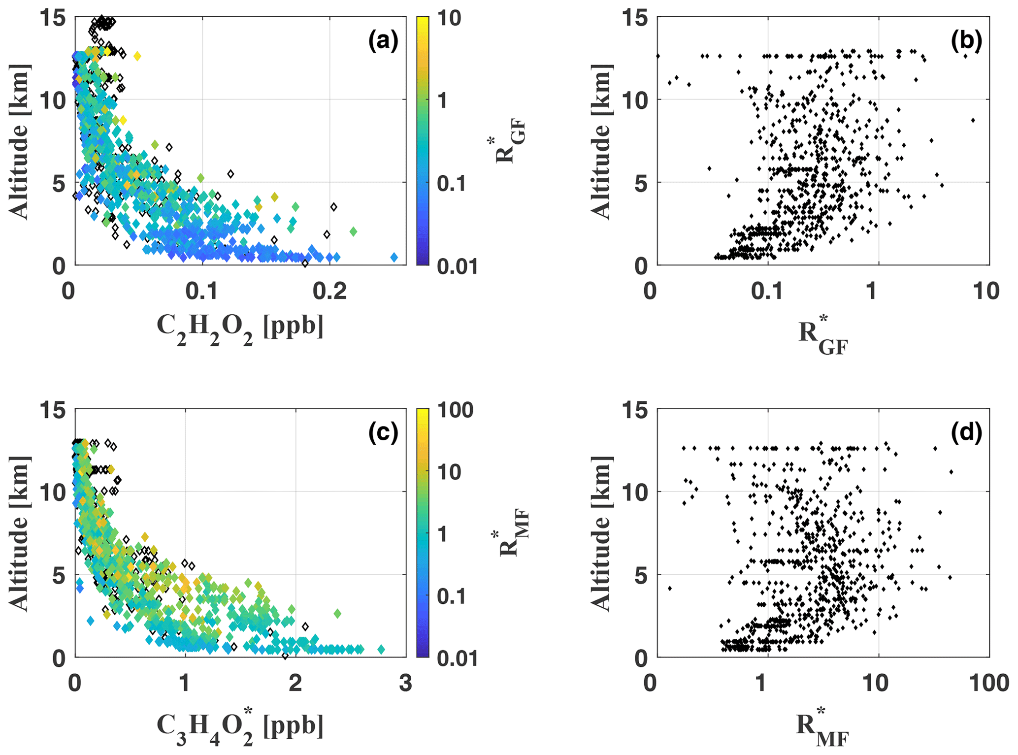
Figure 12 Vertical profiles of C₂H₂O₂ (a) and ${\mathrm{C}}_{\mathrm{3}}{\mathrm{H}}_{\mathrm{4}}{\mathrm{O}}_{\mathrm{2}}^{*}$ (c), colour-coded by the ratios $R_{\mathrm{GF}}^{*}$ and $R_{\mathrm{MF}}^{*}$, respectively, for each measurement during flights AC09, AC11, AC12, and AC13. Black diamonds indicate measurements with missing CH₂O data (recorded with a different spectrometer) and consequently missing ratios. Panels (b) and (d) illustrate the vertical profiles of $R_{\mathrm{GF}}^{*}$ and $R_{\mathrm{MF}}^{*}$ throughout the troposphere. For panels (b) and (d) a logarithmic x axis has been chosen for a better illustration of the altitude dependence of small $R_{\mathrm{GF}}^{*}$ and $R_{\mathrm{MF}}^{*}$ values, respectively.

5.3.1  $R_{\mathrm{GF}}^{*}$

$R_{\mathrm{GF}}^{*}$ mostly remains smaller than 1.0, with a total mean of ${\stackrel{\mathrm{‾}}{R}}_{\mathrm{GF}}^{*}=\mathrm{0.35}\pm \mathrm{0.16}$, but it reaches maximum values >5.0 during several measurements. Small ratios <0.05 and large ratios >1.0 can be observed throughout all analysed flights and nearly all altitudes. The comparison with Kaiser et al. (2015) shows that the inferred $R_{\mathrm{GF}}^{*}$ is notably larger than during most of their in situ measurements at altitudes ranging from the ground up to 6 km over the southeastern US in June–July 2013. Our results are in much better agreement with the $R_{\mathrm{GF}}^{*}$ inferred by MacDonald et al. (2012) from ground-based DOAS measurements for altitudes between 0 and 1000 m over a southeast Asian tropical rainforest in April–July 2008. Their $R_{\mathrm{GF}}^{*}$ in the range from 0.2 to 0.7 agrees with most of our measurements as well as with ${\stackrel{\mathrm{‾}}{R}}_{\mathrm{GF}}^{*}$. From measurements above the Kisatchie National Forest and the Mark Twain National Forest in the southeastern US, Kaiser et al. (2015) conclude characteristically low $R_{\mathrm{GF}}^{*}$ in pristine regions with strong isoprene emissions, while regimes dominated by monoterpene emissions appear to have higher $R_{\mathrm{GF}}^{*}$. Most of our measurements took place in pristine air masses above the rain forest and far away from any major population centre or other anthropogenic emission sources. Monoterpene and isoprene emissions over the central Amazon were studied in multiple investigations (e.g. Helmig et al., 1998 and Kesselmeier et al., 2000). All these studies reported generally low mixing ratios of monoterpenes compared to isoprene, which composes 90 % of the total VOC budget in the Amazon (Kuhn et al., 2007). Apparently, emissions of monoterpenes, like alpha-pinene, are at least 1 order of magnitude smaller than isoprene emissions. Approximately the same relation was found for the total monoterpene emissions (Kuhn et al., 2007; Rizzo et al., 2010). Kaiser et al. (2015) report an approximately 1.2–2.0 times larger C₂H₂O₂ yield from α- and β-pinene oxidation with respect to CH₂O. Still, the significant predominance of isoprene emissions over the Amazon clearly compensates for this effect. We conclude that isoprene and not monoterpenes is the dominant precursor of CH₂O and C₂H₂O₂ for our observations. Contrary to the measurements of Kaiser et al. (2015) in isoprene-rich regimes, the results indicate significantly elevated $R_{\mathrm{GF}}^{*}$ in the troposphere over the Amazon. This is a direct consequence of the much lower CH₂O mixing ratios compared to their measurements over the southeastern US. CH₂O generally does not exceed 1–2 ppb (except for direct measurements in biomass burning or in the Manaus city plume), which is 4 times less than reported by Kaiser et al. (2015) for pristine air masses over the Mark Twain National Forest (ca. 8 ppb). Our C₂H₂O₂ mixing ratios, on the other hand, are comparable to their findings and typically 100 ppt in the lower troposphere. As a result, we obtain significantly higher $R_{\mathrm{GF}}^{*}$ than Kaiser et al. (2015) for the pristine troposphere.

Based on the SENEX observations, Chan Miller et al. (2017) reported mean $R_{\mathrm{GF}}^{*}$ of 0.024 below 1 km altitude. Interestingly, Chan Miller et al. (2017) obtained larger R_GF of up to 0.06 when NO_x was very low (0.1–0.5  ppb). Even though we are not able to infer NO_x concentrations for all measurements due to instrument failures, we were able to measure NO₂ during all analysed flights. Inferred NO₂ mixing ratios from mini-DOAS measurements were very low during all flights. Mixing ratios above 1 ppb were inferred only in rare cases and exclusively over direct emission sources like Manaus city and in biomass fire plumes. We conclude from these overall low NO₂ mixing ratios that the measurements during the campaign were generally under very low-NO_x conditions. As described in detail by Chan Miller et al. (2017), this could lead to prompt glyoxal formation through isoprene peroxy radicals and thus slightly enhanced R_GF compared to observations under high NO_x. Further, from our measurements over Manaus city, we cannot detect any sizable influence of anthropogenic VOCs on the inferred $R_{\mathrm{GF}}^{*}$. During several low overpasses of the city (<2 km flight altitude), $R_{\mathrm{GF}}^{*}$ did not show any significant difference to measurements distant from anthropogenic emission sources. During the measurements in the city plume, the relative increase in CH₂O and C₂H₂O₂ mixing ratios was similar, leading to consistent $R_{\mathrm{GF}}^{*}$.

Finally, the vertical profile of $R_{\mathrm{GF}}^{*}$ indicates slightly elevated ratios above the boundary layer and in the free troposphere (Fig. 12, panel b). Within the boundary layer, $R_{\mathrm{GF}}^{*}$ remains approximately constant. Both features were previously observed by Kaiser et al. (2015) for altitudes up to 6 km, however less pronounced. The increase in $R_{\mathrm{GF}}^{*}$ between 2 and 10 km appears most pronounced just above the boundary layer (at about 2 km), where CH₂O and C₂H₂O₂ mixing ratios are still significantly above the detection limits. Notably, the correlation of CH₂O and C₂H₂O₂ is larger within the boundary layer than in the free troposphere. When discussing the profile shape of $R_{\mathrm{GF}}^{*}$, one has to keep in mind the very low CH₂O and C₂H₂O₂ mixing ratios in the upper troposphere and the increasing influence of measurement noise on the inferred mixing ratios. Above 6 km, we observe mean CH₂O and C₂H₂O₂ of only 54±40 ppt and 15±5 ppt, respectively, and accordingly $R_{\mathrm{GF}}^{*}$ varies on average by 60 % among the different measurements within the same altitude range.

5.3.2  $R_{\mathrm{MF}}^{*}$

Generally, $R_{\mathrm{MF}}^{*}$ appears approximately 10 times larger than $R_{\mathrm{GF}}^{*}$ (Fig. 12, panels c and d). $R_{\mathrm{MF}}^{*}$ values <1 are observed only for a minority of the measurements and mostly for background ${\mathrm{C}}_{\mathrm{3}}{\mathrm{H}}_{\mathrm{4}}{\mathrm{O}}_{\mathrm{2}}^{*}$ concentrations. Larger $R_{\mathrm{MF}}^{*}$ values >1 are inferred at all altitudes, with a total mean ${\stackrel{\mathrm{‾}}{R}}_{\mathrm{MF}}^{*}=\mathrm{3.4}\pm \mathrm{1.6}$ and a maximum ratio $R_{\mathrm{MF},\max }^{*}=\mathrm{45.2}\pm \mathrm{0.8}$. As discussed above for $R_{\mathrm{GF}}^{*}$, the vertical profile of $R_{\mathrm{MF}}^{*}$ indicates slightly larger $R_{\mathrm{MF}}^{*}$ above the boundary layer and throughout the free troposphere. In the upper troposphere, $R_{\mathrm{MF}}^{*}$ decreases again, leading to a concave curvature of the vertical profile for small $R_{\mathrm{MF}}^{*}$ values, as described above for $R_{\mathrm{GF}}^{*}$. Several studies were published on the emission ratio of C₃H₄O₂ to CH₂O (or CO) in biomass burning plumes (e.g. Hays et al., 2002; Müller et al., 2016; Zarzana et al., 2017, 2018). To our knowledge, comparable data for air masses of the free troposphere are not yet available.

5.4 Normalized excess mixing ratios in biomass burning plumes and inferred emission factors

During the four measurement flights, a total of 12 biomass burning plume intercepts were identified based on video imagery (e.g. Fig. 7 for events AC11-1.1/1.2 and AC11-3.1/3.2). Most of the plume measurements occurred south of Manaus and during two extensive flight periods of AC11 and AC13 at altitudes below 2 km. The precise location of all plume intercepts during flight AC11 and the related horizontal averaging kernels of the telescopes are given in Fig. 6. As indicated by the backward trajectories, 3 h prior to detection all probed air masses moved well within the boundary layer, below 600 m altitude. This time frame more than covers the atmospheric lifetimes of CH₂O, C₂H₂O₂, and C₃H₄O₂. Consequently, the measured mixing ratios of these gases are a result of fresh emissions at the surface. Each biomass burning plume encounter correlates with significant enhancements in CH₂O, C₂H₂O₂, and ${\mathrm{C}}_{\mathrm{3}}{\mathrm{H}}_{\mathrm{4}}{\mathrm{O}}_{\mathrm{2}}^{*}$ over the background by 13 % to 400 %. Based on the backward trajectories combined with video imagery and the short lifetimes of the gases, contributions from other major emission sources (e.g. Manaus city) can largely be excluded. The exact timing, location, and altitude of each plume intercept is given in Table 3. As indicated by the numbering in column 1, some of the plumes were probed more than once, giving a total of eight different biomass burning plumes with 12 encounters (further on called events AC11-1.1 to AC13-5). Due to the lack of respective C₂H₂O₂ and C₃H₄O₂ measurements, we infer mean background mixing ratios [X]_bkg for all three gases by binning the data in 100 m altitude stacks and calculating the mean of the lower data quartile for each bin as displayed in Fig. 9 (grey line). As Fig. 10 shows for the case of formaldehyde, the such defined background mixing ratios approximately correspond to formaldehyde measurements of pristine air masses above the western Pacific Ocean by Peters et al. (2012). In order to detect enhancements due to the plumes, [X]_bkg is then subtracted from the measured mixing ratios. From the resulting enhancements, the normalized excess mixing ratio R_XF (or NEMR) is calculated according to

$$\begin{array}{}\text{(4)}& R_{\mathrm{XF}}={\displaystyle \frac{\mathrm{\Delta }\left[X\right]}{\mathrm{\Delta }\left[{\mathrm{CH}}_{\mathrm{2}}\mathrm{O}\right]}}={\displaystyle \frac{\left[X_{\mathrm{fire}}\right]-\left[X_{\mathrm{bkg}}\right]}{[{{\mathrm{CH}}_{\mathrm{2}}\mathrm{O}}_{\mathrm{fire}]}-[{\mathrm{CH}}_{\mathrm{2}}{\mathrm{O}}_{\mathrm{bkg}}]}},\end{array}$$

with X being either C₂H₂O₂ or ${\mathrm{C}}_{\mathrm{3}}{\mathrm{H}}_{\mathrm{4}}{\mathrm{O}}_{\mathrm{2}}^{*}$. The results for each individual biomass burning event as well as the mean and range of R_GF and R_MF are given in Table 3.

Table 3 Inferred normalized excess mixing ratios and emission factors for individual biomass burning events (range and mean). R_GF and R_MF are given in moles per mole. The emission factors EF_G and EF_M are in units of grams per kilogram.

5.4.1  R_GF

R_GF ranges between 0.02 and 0.11, with an average of ${\stackrel{\mathrm{‾}}{R}}_{\mathrm{GF}}=\mathrm{0.07}\pm \mathrm{0.05}$. Repeated measurements of the same biomass burning plumes all agree well within the error, indicating the respective plumes were in fact the major emission sources throughout the measurements. The plume AC11-3 (Fig. 7) yields the highest R_GF of 0.10 and 0.11. Unfortunately, the plume was not reported in the MODIS fire database. Therefore, we do not know the precise location of the fire and cannot discuss the results with respect to the distance of the aircraft from the plume. The smallest R_GF of 0.02 is found during a measurement with an approximately 1000 m higher flight altitude than during the rest of the events.

Our results are consistent with recent laboratory studies on biomass burning emissions by Zarzana et al. (2018) as well as different field measurements and satellite observations by Chan Miller et al. (2014), Chan Miller et al. (2017), DiGangi et al. (2012), Wittrock et al. (2006), and Zarzana et al. (2017). From laboratory measurements, Zarzana et al. (2018) reported an average R_GF of 0.068 for fresh emissions and different kinds of fuels. Without further knowledge on the fuels burned during the observed events, we cannot make firm conclusions on the photochemistry within the fire plumes. While different fuel types may lead to changing emission factors of glyoxal, Zarzana et al. (2018) observed only little variance in R_GF for different burning species. The correlation of C₂H₂O₂ and CH₂O seems to be consistent for different kinds of fuel. The lack of knowledge of the exact fuels burned in each fire is therefore not an issue when comparing R_GF of the different plumes and intercepts. In two older studies, Hays et al. (2002) and McDonald et al. (2000) report much higher R_GF on the order of approximately 2.5 to 3 for Palmae and Poaceae (Hays et al., 2002) and even up to 4 (McDonald et al., 2000). Our inferred R_GF values are at least 1 order of magnitude lower. In fact, results larger than 1 are only observed for the background-uncorrected $R_{\mathrm{GF}}^{*}$ in the free troposphere.

During recent field measurements over the US, Zarzana et al. (2017) report R_GF in the range from 0.008 to 0.11. Due to the very nature of air-borne plume measurements, we do not know by how much the measurements differ with respect to plume age, air mass origin, atmospheric composition, measurement distance to the plume, etc. Despite the very different atmospheric backgrounds and conditions, our measurements over the rain forest agree well with their findings.

Measurements of an aged biomass burning plume yield slightly smaller R_GF values of 0.02 to 0.03 (DiGangi et al., 2012). Of all events, event AC13-5 is most likely the oldest plume measured. This is a consequence of the high flight altitude in combination with the distance from the aircraft to the plume during the measurement. AC13-5 has the smallest R_GF of only 0.02, which agrees with the findings of DiGangi et al. (2012). We cannot state by how much this plume measurement is influenced by the general atmospheric background. The air masses in the boundary layer are generally highly polluted with biomass burning emissions of different ages. We do not know how much these differently aged emissions influenced our individual plume measurements. Therefore, we cannot draw a distinct relationship between R_GF and the plume ages, which due to the well-mixed condition of the boundary layer most probably varied between several minutes to hours during all measurements.

5.4.2  R_MF

R_MF ranges between 0.09 and 1.50, with an average of ${\stackrel{\mathrm{‾}}{R}}_{\mathrm{MF}}=\left(\mathrm{0.98}\pm \mathrm{0.42}\right)$. Three of the eight probed plumes yield R_MF>1 (both measurements of AC11-3, AC13-1, and AC13-2). All the other plumes yield R_MF<1, in the range of 0.09 to 0.86. For event AC11-1, R_GF is comparable to the other results, while R_MF is significantly smaller than the average ${\stackrel{\mathrm{‾}}{R}}_{\mathrm{MF}}$ by approximately a factor of 10. Based on the video imagery, the size of the observed plumes and the estimated distance to the aircraft are comparable during events AC11-1 and AC11-3 (Fig. 7). Still, they yield very different normalized excess mixing ratios. In fact, the largest R_MF and R_GF are obtained during event AC11-3. Accordingly, the emission of C₂H₂O₂ and ${\mathrm{C}}_{\mathrm{3}}{\mathrm{H}}_{\mathrm{4}}{\mathrm{O}}_{\mathrm{2}}^{*}$ with respect to CH₂O is the highest within this biomass burning plume. Interestingly, this is not connected to the size and quantity of the biomass burning events monitored by the telescopes. The highest emissions (i.e. the largest plumes) were observed during event AC11-2, where three different large fires were simultaneously detected in a generally hazy atmosphere rich in fresh emissions (Fig. 7). These plumes were also recorded by MCD14 on MODIS (Fig. 6, red dots in the field of view of event 2.2). Laboratory measurements report R_MF approximately between 1 and 2 for different kinds of fuels (Hays et al., 2002). This is the upper range of our observations. Instead of R_MF, Zarzana et al. (2018) report the ratio of C₃H₄O₂ to C₂H₂O₂ (R_MG) to be on the order of 1.7–2.5 for burning rice straw and different kinds of canopy. Our measurements yield R_MG in the range 1–3, with the exception of event AC11-1, where R_MG<1 due to the small ${\mathrm{C}}_{\mathrm{3}}{\mathrm{H}}_{\mathrm{4}}{\mathrm{O}}_{\mathrm{2}}^{*}$ mixing ratios. Event AC11-3 yields R_MG=1 during both measurements. This reflects the correlated strong enhancement of both gases within the biomass burning plumes.

5.4.3 Biomass burning emission factors

According to Andreae (2019), the biomass burning emission factors for C₂H₂O₂ and ${\mathrm{C}}_{\mathrm{3}}{\mathrm{H}}_{\mathrm{4}}{\mathrm{O}}_{\mathrm{2}}^{*}$ are defined by the normalized excess mixing ratio R_XF as

$$\begin{array}{}\text{(5)}& {\displaystyle }{\mathrm{EF}}_X=R_{\mathrm{XF}}{\displaystyle \frac{{\mathrm{MW}}_X}{{\mathrm{MW}}_{{\mathrm{CH}}_{\mathrm{2}}\mathrm{O}}}}{\mathrm{EF}}_{{\mathrm{CH}}_{\mathrm{2}}\mathrm{O}}\end{array}$$

using the molecular weight (MW) of each species and the mean emission factor ${\mathrm{EF}}_{{\mathrm{CH}}_{\mathrm{2}}\mathrm{O}}$ of the reference trace gas CH₂O. As the latter was not measured during the campaign, we use the recent comprehensive compilation by Andreae (2019), which reports ${\mathrm{EF}}_{{\mathrm{CH}}_{\mathrm{2}}\mathrm{O}}$ with respect to different combustion processes and fuel types. For tropical forest fires, Andreae (2019) inferred mean ${\mathrm{EF}}_{{\mathrm{CH}}_{\mathrm{2}}\mathrm{O}}=\mathrm{2.4}\pm \mathrm{0.63}$. The resulting EF_G and EF_M are listed in Table 3 for each biomass burning plume intercept in units of grams of target species per kilogram of fuel.

EF_G ranges from 0.11 to 0.52 g glyoxal per kilogram of fuel burned with a mean emission factor of $\left(\mathrm{0.25}\pm \mathrm{0.23}\right)\mathrm{g}{\mathrm{kg}}^{-\mathrm{1}}$. According to its high R_GF, event AC11-3 yields the highest emission factors of 0.52 and 0.45 g kg⁻¹. Five out of the 12 plume encounters yield emission factors of less than 0.2 g kg⁻¹. Corresponding to the largest EF_G, Andreae (2019) estimated ${\mathrm{EF}}_{\mathrm{G}}=\mathrm{0.6}\mathrm{g}{\mathrm{kg}}^{-\mathrm{1}}$ for tropical forest fires. In the same study, glyoxal emissions from open burns of agricultural residues were estimated to be approximately 60 % lower with ${\mathrm{EF}}_{\mathrm{G}}=\mathrm{0.23}\mathrm{g}{\mathrm{kg}}^{-\mathrm{1}}$. All biomass burning events encountered during flight AC13 were located between 11.0–11.2^∘ S and 56.2^∘ W. While other parts of the measurement flight were located over rain forest, this region is largely dominated by agricultural activities. EF_G of events AC13-1 to AC13-5 ranges from 0.11 to 0.37 g kg⁻¹. Assuming that the biomass burning plumes were dominated by agricultural residues during these measurements, we infer a corresponding mean emission factor ${\mathrm{EF}}_{\mathrm{G}}=\left(\mathrm{0.25}\pm \mathrm{0.23}\right)$ g glyoxal per kilogram of open burns of agricultural residues. The range of EF_G further agrees with laboratory measurements by Zarzana et al. (2018), who reported EF_G in the range of 0.06 to 0.55 g kg⁻¹ depending on the fuel type.

EF_M ranges between 0.5 and 8.64 g methylglyoxal per kilogram of fuel burned, with a mean emission factor of $\left(\mathrm{4.68}\pm \mathrm{2.7}\right)\mathrm{g}{\mathrm{kg}}^{-\mathrm{1}}$. For each biomass burning event, EF_M is at least twice as high as EF_G. The largest EF_M values were found during flight AC13, i.e. for fires dominated by agricultural residues. Even after applying the correction factor of 2 to the inferred EF_M, the results are significantly larger than reported from laboratory measurements by Zarzana et al. (2018), who found maximal emission factors of approximately 2 g kg⁻¹ for burns of duff. While their absolute EF_M values are much lower, their results were equally variable, with EF_M ranging from 0.11 to 2.0 g kg⁻¹.

6 Conclusions

We report on the first simultaneous measurements of CH₂O, C₂H₂O₂, and ${\mathrm{C}}_{\mathrm{3}}{\mathrm{H}}_{\mathrm{4}}{\mathrm{O}}_{\mathrm{2}}^{*}$ over remote and polluted sections of the Amazon. The measurements were performed from on board the DLR HALO aircraft during the ACRIDICON-CHUVA campaign in autumn 2014 (Wendisch et al., 2016). The observations took place in the troposphere between 500 m and 15 km altitude, where air masses of different compositions were encountered. These include continental background as well as aged and fresh biomass burning plumes.

The observed formaldehyde mixing ratios in the lower and free troposphere range from those previously reported over the remote Pacific (Peters et al., 2012) up to those measured over continental North and South America (Kaiser et al., 2015). The lower quartile of the measured mixing ratios appears to result from the oxidation of methane and to a lesser degree of VOCs (mostly isoprene). In the lower troposphere, enhanced formaldehyde mixing ratios have two major contributions: direct emission, e.g. from biomass burning, and secondary formation during the degradation of short-lived VOCs, like isoprene. In the middle and upper troposphere, formaldehyde seems to have more constant sources and sinks than in the lower troposphere. While the sink (mostly photolysis) may not vary significantly with altitude, the degradation of longer-lived VOCs provides a comparably constant source. When integrating our profiles, our observations are in good agreement with previously inferred formaldehyde VCDs from satellites (De Smedt et al., 2008; Wittrock et al., 2006; Vrekoussis et al., 2010; De Smedt et al., 2015).

A good agreement with previous satellite measurements is also found for the lower and upper ranges of profile-integrated glyoxal mixing ratios (Wittrock et al., 2006; Vrekoussis et al., 2009, 2010; Alvarado et al., 2014). Analogously to the presence of formaldehyde, the lower bound of glyoxal is due to the oxidation of precursor VOCs. Besides direct emissions from biomass burning and secondarily formed glyoxal from short-lived precursors, the oxidation of longer-lived precursors like isoprene or acetone contributes to elevated glyoxal mixing ratios in the free troposphere. Taraborrelli et al. (2020) report in a recent study on long-lived VOCs like aromatics as a potential additional source of glyoxal in the free troposphere on a regional scale. Recent findings by Alvarado et al. (2020) reveal long-range transport of glyoxal and formaldehyde within biomass burning plumes reaching distances of 1500 km downwind and thus enlarging the assumed local influence of biomass burning events on the tropospheric distribution of both gases. The time needed to reach such distances is on the order of several days, which implies the formation of glyoxal and formaldehyde from longer-lived precursors within the plumes.

In agreement with the study of Zarzana et al. (2017), ${\mathrm{C}}_{\mathrm{3}}{\mathrm{H}}_{\mathrm{4}}{\mathrm{O}}_{\mathrm{2}}^{*}$ mixing ratios generally exceed those of glyoxal by at least a factor of 5 during the majority of the measurements. Yet, the shapes of the upper and lower bounds appear similar to the profile shape of glyoxal in contrast to formaldehyde, which appears to decline faster above the boundary layer in the low-NO_x, high-VOC, and low-HO_x environments probed during this study. The compact clustering and the smooth decrease in the lower-quartile mixing ratios with altitude indicate the type and sink of the precursor molecules. Apparently, these precursors should have lifetimes of at least several days and should either be constantly emitted by the biosphere (e.g. isoprene and acetone) or occasionally emitted during biomass burning (e.g. acetylene, aromatics) before being vertically transported. $R_{\mathrm{GF}}^{*}$ and $R_{\mathrm{MF}}^{*}$ are found to increase with altitude due to the more rapid decrease in formaldehyde relative to glyoxal and methylglyoxal mixing ratios. Again, this behaviour expresses the different and changing fractions of the short- and long-lived precursors relevant for the formation of formaldehyde compared to those of glyoxal and methylglyoxal. In particular, the increasing R_GF and R_MF in the middle and upper troposphere require significant sources for both gases which are supposed to result from the oxidation of longer-lived VOCs (Schulz et al., 2018). In fact, since both gases are known to contribute to SOA formation, the elevated mixing ratios of glyoxal and methylglyoxal in the upper troposphere further lend support to the proposed SOA formation from products of isoprene oxidation as observed by Schulz et al. (2018), Andreae et al. (2018), and Williamson et al. (2019) over the Amazon Basin and generally in the tropics.

Our inferred R_GF values in the range of 0.02–0.11 (${\stackrel{\mathrm{‾}}{R}}_{\mathrm{GF}}=\mathrm{0.07}\mathrm{\pm }\mathrm{0.05}$) for the observed biomass burning events agree well with previous studies, both in the field over North America (Zarzana et al., 2017) and in the laboratory fuel study (Zarzana et al., 2018). It is further in agreement with R_GF inferred from satellite measurements (Chan Miller et al., 2014, 2017; DiGangi et al., 2012; Wittrock et al., 2006). For R_MF, we infer a range of 0.09 to 1.5 with ${\stackrel{\mathrm{‾}}{R}}_{\mathrm{MF}}=\mathrm{0.98}$ (or respectively smaller results when correcting the ${\mathrm{C}}_{\mathrm{3}}{\mathrm{H}}_{\mathrm{4}}{\mathrm{O}}_{\mathrm{2}}^{*}$ mixing ratios by a factor of 2.0±0.5), which overlaps with the lower end of the range of normalized excess mixing ratios previously reported by Hays et al. (2002) for different types of fuels in the laboratory. The presented study and the measurements by Hays et al. (2002) indicate a slightly larger R_MF than estimated from R_MG and R_GF (appr. 0.1–0.5) reported by Zarzana et al. (2018), even though this difference may in part be a result of additional dicarbonyls included in our retrieval. In fact, when correcting R_MF by a factor of 2, our results agree much better with the measurements by Zarzana et al. (2018). Based on R_GF and R_MF and average emission factors for formaldehyde estimated by Andreae (2019), we infer emission factors in the range of 0.11–0.52 (${\stackrel{\mathrm{‾}}{\mathrm{EF}}}_{\mathrm{G}}=\left(\mathrm{0.25}\pm \mathrm{0.23}\right)\mathrm{g}{\mathrm{kg}}^{-\mathrm{1}}$) for glyoxal and 0.5–8.6 (${\stackrel{\mathrm{‾}}{\mathrm{EF}}}_{\mathrm{M}}=\left(\mathrm{4.7}\pm \mathrm{2.7}\right)\mathrm{g}{\mathrm{kg}}^{-\mathrm{1}}$) for methylglyoxal for the probed biomass burning events over the Amazon. Our inferred EF_G agrees well with the range reported from laboratory measurements (Zarzana et al., 2018). Notably, our EF_M is significantly larger than found in their study, also when correcting the results for possibly included additional dicarbonyls.

The presented study may be complemented by future studies with data collected during several past HALO missions, i.e. ESMVal (autumn 2012), OMO (over the Mediterranean in summer 2014), EMeRGe (Europe in summer 2017 and eastern Asia in spring 2018), CAFE (over west Africa/tropical Atlantic in summer 2018), and SouthTRAC (southern Argentina and northern Antarctica in autumn 2019), which may provide further information on the role of carbonyls in global atmospheric chemistry.